A method for escaping limit cycles in training GANs

Abstract

This paper mainly conducts further research to alleviate the issue of limit cycling behavior in training generative adversarial networks (GANs) through the proposed predictive centripetal acceleration algorithm (PCAA). Specifically, we first derive the upper and lower bounds on the last-iterate convergence rates of PCAA for the general bilinear game, with the upper bound notably improving upon previous results. Then, we combine PCAA with the adaptive moment estimation algorithm (Adam) to propose PCAA-Adam, a practical approach for training GANs. Finally, we validate the effectiveness of the proposed algorithm through experiments conducted on bilinear games, multivariate Gaussian distributions, and the CelebA dataset, respectively.

97N60, 90C06, 90C25, 90C30

1 Introduction

As of now, generative adversarial networks (GANs) [27] have emerged as a prominent and highly researched topic in the field of deep learning. They hold a crucial position, particularly when it comes to artificial intelligence content generation. Furthermore, they have wide applications in areas such as image generation and editing [16], video generation [61], 3D generation [14, 11], music generation [32], and privacy protection [55]. For more applications, please refer to [56, 10, 41, 62, 20, 2, 55, 65]. The GANs framework consists of two main components: the generator and the discriminator. The generator aims to generate samples that resemble real data, while the discriminator tries to distinguish between samples generated by the generator and real data. These two components compete with each other through adversarial training, ultimately aiming to generate realistic samples. The objective function for adversarial training in GANs can be formulated as follows:

$$\min_{G}\max_{D}V(G,D):=\mathbb{E}_{x\sim\mathbb{P}_{\text{data }}}\big{[}\log D(x)\big{]}+\mathbb{E}_{z\sim\mathbb{P}_{\text{noise}}(z)}\big{[}\log\big{(}1-D\big{(}G(z)\big{)}\big{)}\big{]},$$

where $G$, $D$, $x$ and $z$ represent the generator network, the discriminator network, real data samples drawn from the data distribution $\mathbb{P}_{\text{data}}(x)$, and noise samples drawn from the noise distribution $\mathbb{P}_{\text{noise}}(z)$, respectively. The main goal of adversarial training is to find the optimal generator $G$ that minimizes the discriminator’s ability to distinguish between real and generated samples, while the discriminator $D$ aims to maximize its ability to correctly classify between real and generated samples. For a more detailed understanding of the objective function in GANs, please refer to [27, 26, 63].

Although GANs have many advantages (see [27, 26]) and widespread practical applications (see [21]), they still face numerous challenges both in theory and practical applications (see [26, 50, 59, 12]). One of the most significant challenges is that GANs are hard to train (see [26, 36, 28, 13, 12]), and standard optimization methods often fail to converge to reasonable solution (see [44]). And it has been pointed out in [17, 44] that for practical training of GANs, changes in algorithm outputs are needed for corresponding analysis, and the usual average-iterate convergence is no longer applicable. Therefore, it is necessary to consider the last-iterate convergence of algorithms. However, training GANs using gradient descent ascent (GDA) often shows oscillations and is susceptible to limit cycling behavior in the context of last-iterate convergence (see [17, 52, 9, 60, 53]). Moreover, Lin and Jordan [39] found that for convex-concave games, although [49] established the average-iterate convergence of GDA, GDA may converge to a limit cycle or even diverge in general in the context of last-iterate convergence. Therefore, the training of GANs has been described as “notoriously hard” in [46, 15, 28], highlighting the difficulties associated with this task. In response to these challenges, researchers have recently proposed new algorithms based on GDA to tackle issues encountered during GANs training, including problems like oscillations and limit cycling behavior [17, 52, 37]. Especially, Heish [31] identified how to utilize optimization techniques to eliminate limit cycling behavior in minimax games as an open question, which has attracted researchers to further investigate. Indeed, recently there have been some advances in proposing methods based on GDA to alleviate the limit cycling behavior in training GANs. In particular, Daskalakis et al. [17] were the first to attempt to address the issue of limit cycling behavior in training GANs by introducing optimistic gradient descent ascent (OGDA). Initially, they analyzed the convergence rate of OGDA on the the bilinear game and later integrated OGDA with Adam [34] to propose the Optimistic-Adam algorithm for practical training of GANs. Their numerical experiments with Wasserstein GAN [4] illustrated the superior performance of Optimistic-Adam compared to Adam. Gidel et al. [23] initially demonstrated that OGDA is equivalent to storing and re-using the extrapolated gradient for extrapolation. They then employed variational inequality tools and, assuming monotonicity and compactness and convexity, established the convergence of their proposed “extrapolation from past” algorithm in the average-iteration sense. Finally, they introduced an Adam variant incorporating extrapolation steps for the training of GANs. Mertikopoulos et al. [44] emphasized that adversarial learning, especially concerning GANs, still lacks a comprehensive understanding, and training GANs is widely known to be challenging. Building on the research in [17, 23], Mertikopoulos et al. [44] interpreted the optimistic method as an “extra gradient” step, extrapolating the training process along the current gradient. They established a convergence theory for OGDA, considering dependency and Lipschitz assumptions, and further introduced an alternative version of Optimistic-Adam, showcasing its effectiveness through experiments with DCGAN (see [56]). Moreover, Peng et al. [52] highlighted that training GANs often encounters cyclic behaviors in the iterations. Drawing an analogy with uniform circular motion, they proposed two algorithms, simultaneous centripetal acceleration (Grad-SCA) and alternating centripetal acceleration (Grad-ACA), to mitigate the occurrence of limit cycling behavior. Under suitable assumptions, they derived linear convergence rates for Grad-SCA and Grad-ACA in the bilinear game setting. Additionally, they validated the effectiveness of their proposed RMSprop-ACA algorithm through experiments involving Gaussian kernel learning with GANs. Given the current state of research on GANs training algorithms, directly studying the convergence of training algorithms for GANs is extremely challenging [50, 59, 58]. Therefore, proposing new algorithms that guarantee convergence on simplified GANs models and using them to improve the quality of generated samples in practical applications is of great significance [17, 57, 38, 23, 44, 52, 15, 29]. Taking this into consideration, Li et al. [37] built upon the open question presented in [31] and carried out preliminary investigations in conjunction with GANs. They introduced the predictive centripetal acceleration (PCA) algorithm, which is based on an intuitive geometric interpretation of the approximate centripetal hypothesis. The algorithm demonstrated last-iterate linear convergence on the bilinear game with full-rank square matrices. Additionally, they integrated this algorithm with Adam to propose the PCA-Adam algorithm for the practical training of GANs.

In spite of Li et al. [37] has obtained late-iterate linear convergence results for the bilinear game with the matrix $A$ is a full-rank square matrix, we are curious about the applicability of the algorithm proposed in [37] to more general bilinear game, where the matrix $A$ is not necessarily square. Moreover, we are not satisfied with the linear convergence results achieved in [37], and we wonder if these results can be improved. Furthermore, in order to adapt the algorithms proposed for specific GANs to be used for training general GANs, [37] combines the proposed algorithm with Adam and introduces PCA-Adam. However, we have noticed that the choice of the exponent for the exponential decay rate in PCA-Adam does not make it evident how PCA-Adam can straightforwardly reduce to Extra-Adam [44] and Adam. Therefore, with this purpose in mind, we aim to further investigate and explore the following questions: Q1: Does GDA also diverge when used to solve the general bilinear game? Q2: Does PCAA also converge for the general bilinear game? If it converges, where does the algorithm converge to? Q3: How fast is the convergence rate? Has the convergence rate improved compared to the convergence rate in related literature? Q4: How can we combine the proposed algorithm with Adam in such a way that the resulting new algorithm can simultaneously reduce to both Extra-Adam and Adam? What are the actual effects of the new Adam algorithm proposed in comparison to these two algorithms?

Addressing these questions both theoretically and experimentally constitutes the main research work of this paper. Specifically, firstly, we obtained the result of the PPCA iteration format with a zero projection term for the general bilinear game, which geometrically illustrates the divergence of GDA when used to solve the general bilinear game. Furthermore, based on this result, we can derive the iteration format for PCAA. Secondly, we theoretically proved that if PCAA converges for the general bilinear game in last-iterate sense, the iteration sequence will eventually converge to Nash equilibrium point. Then, we demonstrated that PCAA exhibits linear convergence with a complexity of $\mathcal{O}(\kappa\log(1/\epsilon))$ for the general bilinear game, which improves upon and refines the complexity result of $\mathcal{O}(\kappa^{-2}\log(1/\epsilon))$ obtained in [38] and [37] for the bilinear game with a full-rank matrix. Moreover, we want to emphasize that although the complexity result of PCAA is similar to the literatures [47, 48], the linear convergence results we obtained is superior to the results obtained in [47] and [48]. Furthermore, we have obtained a lower complexity bound of PCAA for the general bilinear game. Finally, we directly combined PCAA with Adam and used the same exponential decay rate for both prediction and update steps in PCAA-Adam. This ensures that PCAA-Adam can easily reduce to Extra-Adam and Adam when certain parameter values are chosen. Furthermore, numerical experiments on the CelebA dataset validated the effectiveness of PCAA-Adam for training GANs compared to Extra-Adam and Adam.

Contributions

• We demonstrate its last-iterate linear convergence on the general bilinear game and provide examples to showcase its effectiveness in alleviating cyclic behavior. Additionally, we provided a lower complexity bound of PCAA for solving the general bilinear game.

• We have identified the reasons for the divergence of GDA in solving the general bilinear game from a geometrically intuitive perspective. Additionally, we analyzed the reasons for non-convergence from the perspective of convergence theory.

• We combined the proposed algorithm PCAA with Anderson mixing and introduced PCAA-AM to accelerate the computational efficiency of PCAA in solving the general bilinear game.

• We combined the proposed algorithm PCAA with Adam and introduced PCAA-Adam for practical training of GANs. Experimental results on the CelebA dataset illustrated that PCAA-Adam outperforms the comparison algorithms such as Adam and Extra-Adam in training GANs.

2 Preliminaries

Throughout this paper, unless otherwise specified, let ${\prod}_{(\theta)}{(\phi)},\;\theta,\phi\in\mathbb{R}^{n}$ denote the projection of vector $\phi$ onto vector $\theta$, $\nabla V(\cdot)$ denote the gradient of function $V$, respectively. A two-player zero-sum game is a game between two players, with one player’s payoff function is denoted by $V$ and the other player’s payoff function is $-V$, where $V:\Theta\times\Phi\rightarrow\mathbb{R}$ with $\Theta\times\Phi\subseteq\mathbb{R}^{m}\times\mathbb{R}^{n}$. The function $V$ maps the actions took by both players $(\theta,\phi)\in\Theta\times\Phi$ to a real value, representing the gain of $\phi$-player and the loss of $\theta$-player. We call $\phi$ player, who tries to maximize the payoff function $V$,the max-player, and $\theta$-player the min-player. In the most classical setting, a two-player zero-sum game has the following form:

$$\min_{\theta\in\Theta}\max_{\phi\in\Phi}V(\theta,\phi).$$

In this paper, we focus on the differentiable two-player game, i.e., payoff functions $V(\cdot,\cdot)$ is differentiable on $\Theta\times\Phi\subseteq\mathbb{R}^{m}\times\mathbb{R}^{n}$.

Definition 2.1 (See [33]).

Point $(\theta^{\star},\phi^{\star})$ is a saddle point of $V$, if for any $(\theta,\phi)\in\Theta\times\Phi$, we have

$$V(\theta^{\star},\phi)\leq V(\theta^{\star},\phi^{\star})\leq V(\theta,\phi^{\star}).$$

Definition 2.2 (See [33]).

Point $(\theta^{*},\phi^{*})$ is referred to as a local saddle point (or local Nash equilibrium point) of the function $V(\cdot,\cdot)$ if there exists $\delta>0$ such that for any $(\theta,\phi)\in\Theta\times\Phi$ satisfying $\|\theta-\theta^{*}\|_{2}\leq\delta$ and $\|\phi-\phi^{*}\|_{2}\leq\delta$, the following inequality holds:

$$V(\theta^{*},\phi)\leq V(\theta^{*},\phi^{*})\leq V(\theta,\phi^{*}).$$

Definition 2.3 (See [1]).

Point $(\theta,\phi)\in\Theta\times\Phi$ is a critical point of the differentiable $V$, if $\nabla V(\theta,\phi)=0$.

3 Predictive centripetal acceleration algorithm

3.1 Related algorithm

A natural approach for players in a differentiable zero-sum game to find a local Nash equilibrium is to use gradient-based search algorithms. The simplest gradient-based algorithm for solving differentiable zero-sum games is the gradient descent ascent (GDA) [46, 52, 6] and its variants such as alternating gradient descent ascent (AGDA) [46, 52, 6] algorithm, extra gradient algorithm (EG) [35], and optimistic gradient descent ascent algorithm (OGDA) [17], among others. These types of algorithms aim to iteratively update the players’ strategies based on gradients, with the goal of converging to a local Nash equilibrium. First, let’s review the iterative formats of GDA and AGDA, where $\alpha$ is the step size parameter.

$$\theta_{t+1}=\theta_{t}-\alpha\nabla_{\theta}V(\theta_{t},\phi_{t}),\quad\phi_{t+1}=\phi_{t}+\alpha\nabla_{\phi}V(\theta_{t},\phi_{t}).$$ (GDA)

$$\theta_{t+1}=\theta_{t}-\alpha\nabla_{\theta}V(\theta_{t},\phi_{t}),\quad\phi_{t+1}=\phi_{t}+\alpha\nabla_{\phi}V(\theta_{t+1},\phi_{t}).$$ (AGDA)

In the following, we review a variant of EG called modified predictive method, proposed by Liang and Stokes in [38], which allows for simultaneous gradient updates. In this variant, referred to as MPM in this article, the parameters $\gamma$ and $\beta$ represent the step sizes for the prediction step and the update step, respectively.

$$\mathrm{Predictive~{}step:}~{}\theta_{t+1/2}=\theta_{t}-\gamma\nabla_{\theta}V(\theta_{t},\phi_{t}),\qquad\phi_{t+1/2}=\phi_{t}+\gamma\nabla_{\phi}V(\theta_{t},\phi_{t});$$ (MPM)

$$\mathrm{gradient~{}step:}~{}\theta_{t+1}=\theta_{t}-\beta\nabla_{\theta}V(\theta_{t+1/2},\phi_{t+1/2});\quad\phi_{t+1}=\phi_{t}+\beta\nabla_{\phi}V(\theta_{t+1/2},\phi_{t+1/2}).$$

Clearly, in algorithm (MPM), if $\gamma=\beta$, then MPM reduces to EG, which was proposed by Korpelevich in [35]. Then, we recall a variant of OGDA called simultaneous centripetal Acceleration (Grad-SCA) and its alternating version Grad-ACA, which were proposed by Peng and Dai et al. in [52], aiming to alleviate the issue of limit cycling behavior in training GANs. The parameters $\alpha_{1},\alpha_{2},\beta_{1},\beta_{2}$ are step size-related parameters. Obviously, in Grad-SCA, when the parameters $\alpha_{1}=\alpha_{2}=\beta_{1}=\beta_{2}$, Grad-SCA reduces to OGDA.

$$G_{\theta}=\nabla_{\theta}V(\theta_{t},\phi_{t})+\frac{\beta_{1}}{\alpha_{1}}\big{(}\nabla_{\theta}V(\theta_{t},\phi_{t})-\nabla_{\theta}V(\theta_{t-1},\phi_{t-1})\big{)}, \theta_{t+1}=\theta_{t}-\alpha_{1}G_{\theta},$$ (Grad-SCA)

$$G_{\phi}=\nabla_{\phi}V(\theta_{t},\phi_{t})+\frac{\beta_{2}}{\alpha_{2}}\big{(}\nabla_{\phi}V(\theta_{t},\phi_{t})-\nabla_{\phi}V(\theta_{t-1},\phi_{t-1})\big{)}, \phi_{t+1}=\phi_{t}+\alpha_{2}G_{\phi}.$$

$$G_{\theta}=\nabla_{\theta}V(\theta_{t},\phi_{t})+\frac{\beta_{1}}{\alpha_{1}}\big{(}\nabla_{\theta}V(\theta_{t},\phi_{t})-\nabla_{\theta}V(\theta_{t-1},\phi_{t-1})\big{)}, \theta_{t+1}=\theta_{t}-\alpha_{1}G_{\theta},$$ (Grad-ACA)

$$G_{\phi}=\nabla_{\phi}V(\theta_{t+1},\phi_{t})+\frac{\beta_{2}}{\alpha_{2}}\big{(}\nabla_{\phi}V(\theta_{t+1},\phi_{t})-\nabla_{\phi}V(\theta_{t},\phi_{t-1})\big{)}, \phi_{t+1}=\phi_{t}+\alpha_{2}G_{\phi}.$$

Finally, we present an example to visually demonstrate the oscillation and limit cycle problems that exist when using GDA to solve two-player zero-sum games. Please refer to Figure 1 for details.

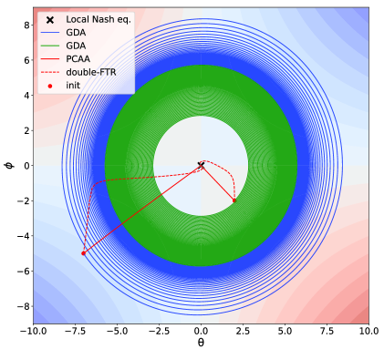
(a) $V(\theta,\phi)=\theta\phi+\epsilon(\theta^{2}-\phi^{2})$

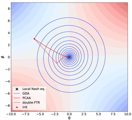
(b) $V(\theta,\phi)=2\theta^{2}-50\theta\phi-\phi^{2}$

Figure 1: Two examples of issues with GDA in finding Nash equilibrium in zero-sum games, where the double-FTR algorithm can be found in [8]. (a) GDA converges to a limit cycle (we use $\epsilon=0.0001,\gamma=\beta=0.01,\alpha=0$) instead of the unique Nash equilibrium $(0,0)$. (b) The convergence process of GDA exhibits oscillations, manifested as a slow spiral convergence towards the Nash equilibrium.

In response to the issue of limit cycling behavior and inspired by the work in [17], Peng et al. [52] proposed the SCA and ACA methods to alleviate such behavior. Especially, they provided an explanation of the fundamental intuition behind centripetal acceleration in [52, Figure 1]. First, they considered uniform circular motion, where $\nabla V_{t}$ represents the instantaneous velocity at time $t$. The centripetal acceleration $\lim_{\delta t\rightarrow 0}(\nabla V_{t+\delta t}-\nabla V_{t})/\delta t$ points towards the origin. And they argued that the cyclic behavior around a Nash equilibrium may resemble circular motion around the origin. Then, they proposed that the centripetal acceleration provides a direction along which the iterates can approach the target more quickly. Finally, they utilized $(\nabla V_{t+\delta t}-\nabla V_{t})$, referred to as the approximate centripetal acceleration term, to approximate $\lim_{\delta t\rightarrow 0}(\nabla V_{t+\delta t}-\nabla V_{t})/\delta t$, and this approximated term is applied to modify GDA resulting in Grad-SCA.

A natural idea of this work and [37] is to explore how to understand the approximate centripetal acceleration method geometrically and how to construct a direction that directly points to the origin to alleviate limit cycling behavior, instead of employing the approximated centripetal acceleration term?

Motivated by the above question and inspired by OGDA, Grad-SCA, MPM and lookahead methods [15, 68], we also considered the uniform circular motion, as shown in Figure 2 below. Let $\nabla V_{t}$ denote the instantaneous velocity at time $t$. Firstly, we performed a prediction step at $t+1/2$, and obtain the instantaneous velocity $\nabla V_{t+1/2}$ at that time. Then, we computed the approximated centripetal acceleration term $(\nabla V_{t+1/2}-\nabla V_{t})$ at time $t$. Finally, we projected the approximated centripetal acceleration term $(\nabla V_{t+1/2}-\nabla V_{t})$ at time $t$ onto $\nabla V_{t}$, the instantaneous velocity at time $t$. By doing so, we obtained the projection centripetal acceleration term ${\prod}_{\big{(}\nabla V(\theta_{t},\phi_{t})\big{)}}{\big{(}\nabla V(\theta_{t+1/2},\phi_{t+1/2})-\nabla V(\theta_{t},\phi_{t})\big{)}}$, which precisely points to the origin. For more details, see Figure 2. We also argued that the cyclic behavior around a Nash equilibrium might be similar to the circular motion around the origin. Therefore, the projection centripetal acceleration term provides a direction, along which the iterates can approach the target directly. Then the projection centripetal acceleration term is also applied to modify GDA.

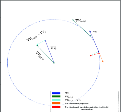
(a)

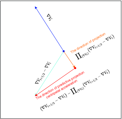
(b)

Figure 2: (a): The basic intuition of predictive projection centripetal acceleration methods in this work and [37]. (b): It provides a magnified view and description of the projection term $\prod_{(\nabla V_{t})}{(\nabla V_{t+1/2}-\nabla V_{t})}$, which represents the projection of $\nabla V_{t+1/2}-\nabla V_{t}$ onto $\nabla V_{t}$. Additionally, it shows the projection centripetal acceleration term $(\nabla V_{t+1/2}-\nabla V_{t})-\prod_{(\nabla V_{t})}{(\nabla V_{t+1/2}-\nabla V_{t})}$ in subfigure (a).

Finally, we obtained the predictive projection centripetal acceleration algorithm (PPCA) in [37] with the following form :

$${\mathrm{Predictive~{}step:}}~{}\theta_{t+1/2}=\theta_{t}-\gamma\nabla_{\theta}V(\theta_{t},\phi_{t}),\phi_{t+1/2}=\phi_{t}+\gamma\nabla_{\phi}V(\theta_{t},\phi_{t});$$ (1)

$${\mathrm{gradient~{}step:}}~{}\bigg{(}\begin{array}[]{c}\theta_{t+1}\\ \phi_{t+1}\end{array}\bigg{)}=\bigg{(}\begin{array}[]{c}\theta_{t}\\ \phi_{t}\end{array}\bigg{)}+\alpha\nabla\bar{V}(\theta_{t},\phi_{t})+\beta\bigg{(}\big{(}\nabla\bar{V}(\theta_{t+1/2},\phi_{t+1/2})-\nabla\bar{V}(\theta_{t},\phi_{t})\big{)}$$

$${\qquad\qquad\qquad\qquad\qquad\qquad\qquad\qquad}-{\prod}_{\big{(}\nabla\bar{V}(\theta_{t},\phi_{t})\big{)}}{\big{(}\nabla\bar{V}(\theta_{t+1/2},\phi_{t+1/2})-\nabla\bar{V}(\theta_{t},\phi_{t})\big{)}}\bigg{)},$$

where $\nabla\bar{V}(\theta_{t},\phi_{t}):=\bigg{(}\begin{array}[]{c}-\nabla{V}_{\theta}(\theta_{t},\phi_{t})\\ \nabla{V}_{\phi}(\theta_{t},\phi_{t})\end{array}\bigg{)}$, and ${\prod}_{\big{(}\nabla\bar{V}(\theta_{t},\phi_{t})\big{)}}{\big{(}\nabla\bar{V}(\theta_{t+1/2},\phi_{t+1/2})-\nabla\bar{V}(\theta_{t},\phi_{t})\big{)}}$ denotes the projection of vector ${\nabla\bar{V}(\theta_{t+1/2},\phi_{t+1/2})-\nabla\bar{V}(\theta_{t},\phi_{t})}$ onto vector ${\nabla\bar{V}(\theta_{t},\phi_{t})}$.

3.2 Predictive centripetal acceleration algorithm

The study on the bilinear game can reveal the fundamental issues of gradients in games [7]. Moreover, the bilinear game is often used as a simple model for theoretical discussions on the reasons behind problems in training GANs [5], and they serve as important illustrative examples for analyzing and understanding new algorithms and techniques [17, 22, 23, 24, 38, 66]. In fact, the bilinear game can reveal the challenges that GDA encounters in training GANs, and it can represent some simple forms of GANs [54, 17, 23, 45]. Moreover, since Goodfellow [26] analyzed the circular trajectories of GDA on the two-dimensional bilinear game in 2016, almost all research on proposing new algorithms based on GDA has discussed the bilinear game to demonstrate the effectiveness of the proposed algorithms. In addition to the references mentioned above, recent research papers include [25, 19, 23, 66, 40, 3], among others. Especially, following the research approach of the aforementioned papers, Li et al. [37] discussed the properties of PPCA under the condition that the matrix is a full-rank square matrix. However, for a more general scenario where the matrix is not necessarily square, this aspect has not been explored yet. Therefore, the main focus of this paper is to investigate the properties of PPCA in the context of the bilinear game with a matrix that is not necessarily square.

In this section, we first discuss a property of algorithm (1) on the following bilinear game. This property is helpful for understanding the performance of GDA in game and simplifying the iterative format of algorithm (1).

$$\min_{\theta\in\mathbb{R}^{m}}\max_{\phi\in\mathbb{R}^{n}}\theta^{\mathrm{T}}A\phi+\theta^{\mathrm{T}}b+c^{\mathrm{T}}\phi,\quad A\in\mathbb{R}^{m\times n},\quad b\in\mathbb{R}^{m},\,c\in\mathbb{R}^{n},$$ (2)

where $\theta\in\mathbb{R}^{m},\,\phi\in\mathbb{R}^{n}$ implies that $\theta$-player and $\phi$-player have different decision spaces. By the first order conditions of the game defined by (2), we have

$$\begin{array}[]{rc}A\phi^{{}^{\prime}}+b&=0,\\ A^{\mathrm{T}}\theta^{{}^{\prime}}+c&=0,\end{array}$$

where $(\theta^{{}^{\prime}},\phi^{{}^{\prime}})$ is a critical point of game (2). If $b$ (resp. $c$) does not belong to the column space of $A$ (resp. $A^{\mathrm{T}}$), then game (2) has no Nash equilibrium. In the following, drawing inspiration from the approach outlined in [47, 24, 66], we also make the assumption that a Nash equilibrium exists for this game. As a result, there exist $\bar{\phi}$ and $\bar{\theta}$ such that $b=-A\bar{\phi}$ and $c=-A^{\mathrm{T}}\bar{\theta}$. Then, we transform $(\theta,\phi)$ to $(\theta-\bar{\theta},\phi-\bar{\phi})$, thus game (2) is reformulated as:

$$\min_{\theta\in\mathbb{R}^{m}}\max_{\phi\in\mathbb{R}^{n}}V(\theta,\phi)=\theta^{\mathrm{T}}A\phi,\quad A\in\mathbb{R}^{m\times n}.$$ (3)

Then, we present the following proposition, which is crucial for deriving our main algorithm and proving its convergence on zero-sum game (3).

Proposition 3.1.

If $A$ is a non-zero matrix in bilinear game (3), and $\nabla\bar{V}(\theta_{t},\phi_{t})\neq 0$, then the projection term of the iterative format for PPCA in (1) is zero.

The proof is similar to Lemma 3.1 in [37], so it is omitted here.

Proposition 3.1 states that for game (3) with non-zero matrix $A$, the approximate centripetal acceleration term $\nabla\bar{V}(\theta_{t+1/2},\phi_{t+1/2})-\nabla\bar{V}(\theta_{t},\phi_{t})$ is orthogonal to $\nabla\bar{V}(\theta_{t},\phi_{t})$. Therefore, the approximate centripetal acceleration term $\nabla\bar{V}(\theta_{t+1/2},\phi_{t+1/2})-\nabla\bar{V}(\theta_{t},\phi_{t})$ directly points towards the center’s direction at time $t$ with any non-zero predictive step size $\gamma$. Therefore, combining Proposition 1 in [17], we have the following remark.

Remark 3.2.

[17, Proposition 1] states that when using GDA to solve bilinear game $\min_{\theta\in\mathbb{R}^{n}}\max_{\phi\in\mathbb{R}^{n}}$ $\theta^{\mathrm{T}}\phi$, for any initial point $(\theta_{0},\phi_{0})$ satisfying $\theta_{0},\phi_{0}\neq 0$, the iteration process diverges. Motivated by [17, Proposition 1], this paper raises the following questions: “How to geometrically understand the Proposition 1? And for game (3) with a non-zero matrix $A\in\mathbb{R}^{m\times n}$, does GDA also diverge in terms of last-iterate sense?”

In fact, Proposition 3.1 answers the above two questions. According to Proposition 3.1, $\nabla\bar{V}(\theta_{t},\phi_{t})$, $\nabla\bar{V}(\theta_{t+1/2},\phi_{t+1/2})$, and $\nabla\bar{V}(\theta_{t+1/2},\phi_{t+1/2})-\nabla\bar{V}(\theta_{t},\phi_{t})$ form a right-angled triangle with $\nabla\bar{V}(\theta_{t},\phi_{t})$ and $\nabla\bar{V}(\theta_{t+1/2},\phi_{t+1/2})-\nabla\bar{V}(\theta_{t},\phi_{t})$ as the perpendicular sides, and $\nabla\bar{V}(\theta_{t+1/2},\phi_{t+1/2})$ as the hypotenuse. This means that when using GDA to solve the game mentioned above, after each iteration, the magnitude of gradient $\nabla\bar{V}(\theta_{t+1},\phi_{t+1})$ at the next iteration point continuously increases relative to gradient $\nabla\bar{V}(\theta_{t},\phi_{t})$ at the current step. Therefore, GDA diverges on bilinear game (3). Theorem 3.1 geometrically explains Proposition 1 in [17]. Simultaneously, Theorem 3.1 provides a geometric interpretation of the fact that when using GDA to solve game $\min_{\theta\in\mathbb{R}^{m}}\max_{\phi\in\mathbb{R}^{n}}\theta^{\mathrm{T}}A\phi$, with any initial point $(\theta_{0},\phi_{0})$ satisfying $\theta_{0},\phi_{0}\neq 0$, it diverges, where $A$ is a non-zero matrix.

Moreover, from Proposition 3.1, we see that the projection term of in algorithm (1) is zero. Thus, algorithm (1) has the following simple form on bilinear game (3).

$$\begin{split}{\rm Predictive~{}step:}\quad\theta_{t+1/2}&=\theta_{t}-\gamma\nabla_{\theta}V(\theta_{t},\phi_{t}),\\ \phi_{t+1/2}&=\phi_{t}+\gamma\nabla_{\phi}V(\theta_{t},\phi_{t});\\ {\rm gradient~{}step:}\quad\theta_{t+1}&=\theta_{t}-\alpha\nabla_{\theta}V(\theta_{t},\phi_{t})-\beta\big{(}\nabla V_{\theta}(\theta_{t+1/2},\phi_{t+1/2})-\nabla V_{\theta}(\theta_{t},\phi_{t})\big{)},\\ \phi_{t+1}&=\phi_{t}+\alpha\nabla V_{\phi}(\theta_{t},\phi_{t})+\beta\big{(}\nabla V_{\phi}(\theta_{t+1/2},\phi_{t+1/2})-\nabla V_{\phi}(\theta_{t},\phi_{t})\big{)}.\end{split}$$ (4)

In this paper, we will refer to this algorithm as the predictive centripetal acceleration algorithm (PCAA). Given its simplicity and effectiveness in the test examples, we have chosen to study it as the main algorithm for our research. Additionally, it is easy to observe that by adjusting GDA to different extents using the approximate centripetal acceleration term, we can obtain algorithms named OGDA, GOGDA in [48], and Grad-SCA, respectively. Therefore, combining Proposition 3.1, the following remark can be obtained, which can also be found in [37].

Remark 3.3 ([37]).

Although the idea of PCAA originates from OGDA, GOGDA, and Grad-SCA, while PCAA still differs from them, primarily in terms of how they adjust GDA. OGDA, GOGDA, and Grad-SCA use the approximate centripetal acceleration term at time $t$, $\nabla\bar{V}(\theta_{t+1},\phi_{t+1})-\nabla\bar{V}(\theta_{t},\phi_{t})$, to adjust the algorithm’s performance at time $t+1$. In contrast, PCAA first obtains the gradient information for the predictive step and then uses this information to adjust the algorithm’s performance at time $t$ in the direction pointing towards the center. Specifically, according to Theorem 3.1, this difference is particularly pronounced in case of bilinear game (3).

Next, we provide the following relationships regarding the parameters in iterative formats between PCAA and GDA, EG and MPM, which can also be found in [37].

Remark 3.4 ([37]).

It is evident that if $\gamma=0,\alpha\neq 0$ or $\beta=0,\alpha\neq 0$ in PCAA iterative format (4), then PCAA is equivalent to GDA. Additionally, if $\beta=\alpha\neq 0$ in (4), then PCAA will be reduced to MPM. Furthermore, if $\beta=\alpha=\gamma$ in (4), then PCAA is equivalent to EG.

Finally, we conducted comparative experiments on the example in [8] to illustrate the effectiveness of PCAA in terms of avoiding spurious critical points and oscillatory behavior near local Nash equilibria. For specific experimental details, please refer to Figure 3.

(a)

(b)

(c)

Figure 3: (a): Evolution of GDA, double-FTR and PCAA in the 2-D toy example from multiple initial points. (b): Zoom-in near a local Nash equilibrium point. (c): Zoom-in near a non-Nash LASE for the GDA algorithm. The definitions of LASE and LSS can be found in [8].

As shown in Figure 3, while GDA may converge to critical points that are not local Nash equilibria, PCAA can avoid such spurious critical points. Additionally, GDA exhibits oscillatory behavior near local Nash equilibria, whereas PCAA does not have oscillatory behavior near local Nash equilibria. For reference, we also show the trajectories of Local Symplectic Surgery (LSS) [42], as mentioned in [8].

4 Two illustrative examples

4.1 An illustrative example: Learning the mean of a multivariate Gaussian distribution.

The third part of [17] considers a simple Wasserstein GAN example, where data is generated from a multivariate normal distribution, i.e. $Q\triangleq{N}(v,I)$ for some $v\in\mathbb{R}^{n}$. The purpose is to enable the generator to learn the unknown parameter $v$. The specific details are as follows.

Consider a Wasserstein GAN, where the discriminator is a linear function and the generator is an additive shift of the input noise $z$, where the noise $z$ is sampled from the distribution $F\triangleq{N}(0,I)$, i.e.

$$D_{\phi}(x)=\langle\phi,x\rangle,\quad G_{\theta}(z)=z+\theta.$$

The goal of the generator is to approximate the true distribution, i.e., for $\theta$ to converge to $v$. The loss function of the Wasserstein GAN takes the following form:

$$L(\theta,\phi)=\mathbb{E}_{x\sim{N}(v,I)}[\langle\phi,x\rangle]-\mathbb{E}_{z\sim{N}(0,I)}[\langle\phi,z+\theta\rangle].$$

Consider a scenario where we optimize the true expectation mentioned above instead of assuming only samples of $x$ and $z$. Given the linearity property of expectations, the expected zero-sum game takes the following form:

$$\inf_{\theta}\sup_{\phi}\langle\phi,v-\theta\rangle.$$ (5)

For more detailed derivations regarding the loss function, please refer to [17]. Note that the equilibrium point of above game (5) is unique, namely the generator parameters are $v=\theta$ and the discriminator parameters are $\phi=0$. For this simple zero-sum game, we have $\nabla_{\mathbf{\phi}}L=v-\theta$ and $\nabla_{\mathbf{\theta}}L=-\phi$. Therefore, the iterative format for GDA is as follows:

$$\phi_{t+1}=\phi_{t}+\eta(v-\theta_{t}),\quad\theta_{t+1}=\theta_{t}+\eta\phi_{t}.$$

The iterative format for OGDA is as follows:

$$\phi_{t+1}=\phi_{t}+2\eta(v-\theta_{t})-\eta(v-\theta_{t-1}),\quad\theta_{t+1}=\theta_{t}+2\eta\phi_{t}-\eta\phi_{t-1}.$$

The iterative format for MPM is as follows:

$$\phi_{t+1/2}=\phi_{t}+\gamma(v-\theta_{t}),\qquad\theta_{t+1/2}=\theta_{t}+\gamma\phi_{t};$$

$$\phi_{t+1}=\phi_{t}+\beta(v-\theta_{t+1/2}),\quad\theta_{t+1}=\theta_{t}+\beta\phi_{t+1/2}.$$

While the iterative format for PCAA in this paper is as follows:

$$\phi_{t+1/2}=\phi_{t}+\gamma(v-\theta_{t}),\quad\quad\quad\quad\quad\quad\quad~{}~{}\theta_{t+1/2}=\theta_{t}+\gamma\phi_{t};$$

$$\phi_{t+1}=\phi_{t}+\alpha(v-\theta_{t})-\beta(\theta_{t+1/2}-\theta_{t}),\quad\theta_{t+1}=\theta_{t}+\alpha\phi_{t}+\beta(\phi_{t+1/2}-\phi_{t}).$$

The effectiveness of OGDA in alleviating the issue of limit cycling behavior is demonstrated in Section 3 of [17], using Wasserstein GAN as an example. Inspired by the work of [17], this paper compares the numerical performance of several algorithms in mitigating limit cycling behavior using the same example, highlighting that PCAA is more effective than other methods in addressing the issue of limit cycling behavior.

We proceed with simultaneous training on zero-sum game (5) using GDA, OGDA, MPM and PCAA. It is noted in [17] that the GDA iteration process exhibits limit cycling behavior regardless of the step size or other modifications. Figure 4 to Figure 5 display the dynamic behavior of GDA, OGDA, MPM, and PCAA on this game when $v=(3,4)$.

(a) GDA dynamics

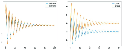
(b) OGDA dynamics

Figure 4: A reproduction of the results from Figure 1 in [17]. (a): Training this Wasserstein GAN using GDA converges to a limit cycle around the equilibrium point. To prevent the GDA iteration process from cycling, the weight clipping technique is applied to the discriminator parameters during training. (b): Training Wasserstein GAN using OGDA converges to an equilibrium point in the last-iterate convergence.

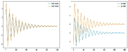
(a) MPM dynamics

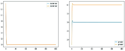
(b) PCAA dynamics

Figure 5: (a):Training the Wasserstein GAN using MPM leads to convergence in the sense of the last-iterate convergence, but the algorithm exhibits slight oscillations. (b): Training the Wasserstein GAN using PCAA results in convergence in terms of the last-iterate convergence, and the iteration process shows almost no oscillations or limit cycling behavior.

The horizontal axis in Figure 4 and Figure 5 represents the number of iterations, while the vertical axis represents the corresponding values for the generator or discriminator. From the results of the four experiments mentioned above, it can be observed that the GDA dynamic leads to limit cycling behavior (although it does converge to the true vector $v$ in the average sense) in this game. On the other hand, OGDA, MPM, and PCAA dynamics can converge to the true vector $v$ in terms of last-iterate sense. However, OGDA and MPM dynamics exhibit slight oscillations, while the PCAA dynamic shows almost no oscillation. Furthermore, Daskalakis et al. [17] pointed out that improving the stability of the GDA dynamic can be achieved by adding a gradient penalty term to the GDA iteration scheme, introducing Nesterov momentum, or updating the generator once and the discriminator multiple times. However, unlike OGDA, these methods only narrow down the range of limit cycles, and the limit cycling behavior still persists. In fact, comparing the variation of oscillation amplitude with the number of iterations in the four experiments mentioned above, it can be observed that when OGDA, MPM, and PCAA have the same corresponding parameters, PCAA exhibits better numerical performance in alleviating the limit cycling behavior compared to OGDA and MPM.

4.2 Another example: Learning a co-variance matrix.

This part demonstrates the effectiveness of PCAA in alleviating the limit cycling behaviors through an example of learning the covariance matrix of a multivariate Gaussian distribution. The problem description in this section is similar to that in [17]. It assumes that the data distribution follows a multivariate normal distribution with zero mean and an unknown covariance matrix, i.e., $x\sim N(0,\Sigma)$. Now, let’s consider the case where the discriminator is a quadratic function, i.e.,

$$D_{W}(x)=\sum_{ij}W_{ij}x_{i}x_{j}=x^{\mathrm{T}}Wx,$$

The generator is a linear function of the input random noise, denoted as $z\sim N(0,I)$, and is defined as follows:

$$G_{V}(z)=Vz,$$

where $W,V\in\mathbb{R}^{n\times n}$. The Wasserstein GAN loss function with the aforementioned generator and discriminator is given by:

$$L(V,W)=\mathbb{E}_{x\sim N(0,\Sigma)}\left[x^{\mathrm{T}}Wx\right]-\mathbb{E}_{z\sim N(0,I)}\left[z^{\mathrm{T}}V^{\mathrm{T}}WVz\right].$$ (6)

Expanding the loss function (6) and assuming that the covariance matrix is a positive definite matrix, which can be obtained through Cholesky decomposition as $\Sigma=UU^{\mathrm{T}}$, then the loss function (6) can be simplified to:

$$L(V,W)=\sum_{ij}W_{ij}\bigg{(}\Sigma_{ij}-\sum_{k}V_{ik}V_{jk}\bigg{)}=\sum_{ijk}W_{ij}\bigg{(}U_{ik}U_{jk}-V_{ik}V_{jk}\bigg{)}.$$

For more detailed derivations regarding the loss function, please refer to [17]. Consider the iteration process of the algorithm without sampling noise. Then, The GDA update rule for this example is as follows:

$$W_{t}=W_{t-1}+\alpha\big{(}\Sigma-V_{t-1}V_{t-1}^{\mathrm{T}}\big{)},\quad V_{t}=V_{t-1}+\alpha\big{(}W_{t-1}+W_{t-1}^{\mathrm{T}}\big{)}V_{t-1}.$$

Similarly, the OGDA update rule can be written as follows:

$$W_{t} =W_{t-1}+2\alpha\big{(}\Sigma-V_{t-1}V_{t-1}^{\mathrm{T}}\big{)}-\alpha\big{(}\Sigma-V_{t-2}V_{t-2}^{\mathrm{T}}\big{)},$$

$$V_{t} =V_{t-1}+2\alpha\big{(}W_{t-1}+W_{t-1}^{\mathrm{T}}\big{)}V_{t-1}-\alpha\big{(}W_{t-2}+W_{t-2}^{\mathrm{T}}\big{)}V_{t-2}.$$

The MPM update rule can be written as follows:

$$W_{t-1/2}=W_{t-1}+\gamma\big{(}\Sigma-V_{t-1}V_{t-1}^{\mathrm{T}}\big{)},V_{t-1/2}=V_{t-1}+\gamma\big{(}W_{t-1}+W_{t-1}^{\mathrm{T}}\big{)}V_{t-1};$$

$$W_{t}=W_{t-1}+\alpha\big{(}\Sigma-V_{t-1/2}V_{t-1/2}^{\mathrm{T}}\big{)},V_{t}=V_{t-1}+\alpha\big{(}W_{t-1/2}+W_{t-1/2}^{\mathrm{T}}\big{)}V_{t-1/2}.$$

The PCAA update rule can be written as follows:

$$W_{t-1/2}=W_{t-1}+\gamma\big{(}\Sigma-V_{t-1}V_{t-1}^{\mathrm{T}}\big{)},\quad V_{t-1/2}=V_{t-1}+\gamma\big{(}W_{t-1}+W_{t-1}^{\mathrm{T}}\big{)}V_{t-1};$$

$$W_{t}=W_{t-1}+\alpha\big{(}\Sigma-V_{t-1}V_{t-1}^{\mathrm{T}}\big{)}+\beta\bigg{(}\big{(}\Sigma-V_{t-1/2}V_{t-1/2}^{\mathrm{T}}\big{)}-\big{(}\Sigma-V_{t-1}V_{t-1}^{\mathrm{T}}\big{)}\bigg{)},$$

$$V_{t}=V_{t-1}+\alpha\big{(}W_{t-1}+W_{t-1}^{\mathrm{T}}\big{)}V_{t-1}+\beta\bigg{(}\big{(}W_{t-1/2}+W_{t-1/2}^{\mathrm{T}}\big{)}V_{t-1/2}-\big{(}W_{t-1}+W_{t-1}^{\mathrm{T}}\big{)}V_{t-1}\bigg{)}.$$

The two experiments below provided the weights of the discriminator and generator distributions, as well as the hidden covariance matrix $\Sigma=VV^{\mathrm{T}}$, at each iteration step, respectively, on two-dimensional and three-dimensional Gaussian distributions. Comparing the oscillation amplitudes with the number of iterations in the experimental results, it was found that PCAA performed better in terms of stabilizing the training process compared to the other three algorithms. What needs to be clarified is that in Figure 6 and Figure 7, the x-axis represents the number of iterations, while the y-axis represents the numerical values corresponding to each component of the generator, discriminator, and covariance matrix.

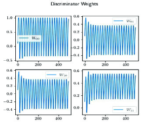
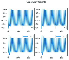
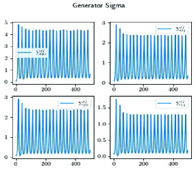
(a) GDA dynamics with $\alpha=0.1,T=500,\lambda=0.4$.

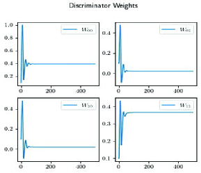
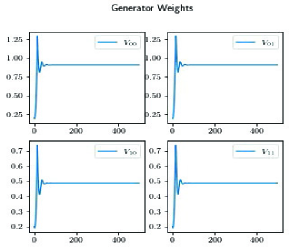
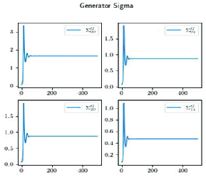
(b) OGDA dynamics with $\alpha=0.1,T=500,\lambda=0.4$.

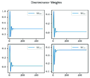
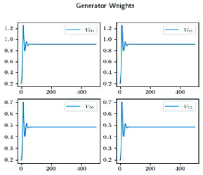
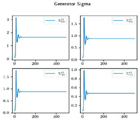
(c) MPM dynamics with $\gamma=\alpha=0.1,T=500,\lambda=0.4$.

(d) PCAA dynamics with $\gamma=\alpha=0.1,\beta=0.07,T=500,\lambda=0.4$.

Figure 6: Subfigure (a) to (d) present comparative experiments on the stability of GDA, OGDA, MPM, and PCA in covariance matrix learning for a two-dimensional Gaussian distribution ($d=2$). Weight clipping in [-1,1] was applied in four dynamics.

By comparing the oscillation amplitudes with the number of iterations in Figure 6, it can be observed that in the covariance matrix learning problem of the two-dimensional Gaussian distribution, OGDA, MPM, and PCAA all effectively alleviate the issue of limit cycles.

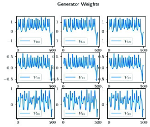
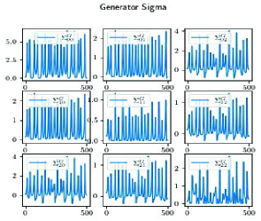
(a) GDA dynamics with $\alpha=0.1,T=500,\lambda=0.4$.

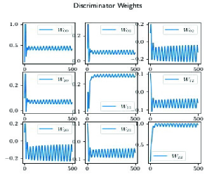
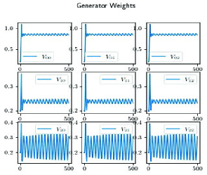
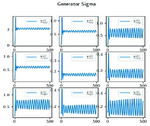
(b) OGDA dynamics with $\alpha=0.1,T=500,\lambda=0.4$.

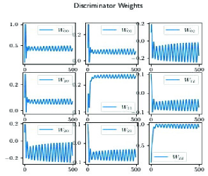
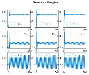
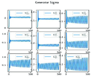
(c) MPM dynamics with $\gamma=\alpha=0.1,T=500,\lambda=0.4$.

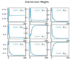
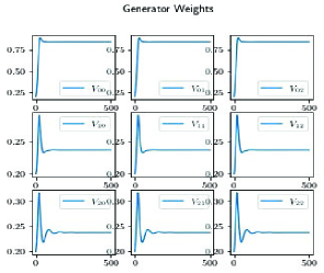
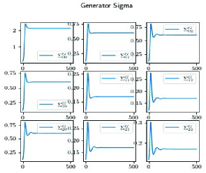
(d) PCAA dynamics with $\gamma=\alpha=0.1,\beta=0.04,T=500,\lambda=0.4$.

Figure 7: Subfigure (a) to (d) present comparative experiments on the stability of GDA, OGDA, MPM, and PCA in covariance matrix learning for a three-dimensional Gaussian distribution ($d=3$). Weight clipping in [-1,1] was applied in four dynamics. Weight clipping in [-1,1] was applied in four dynamics.

Although all three methods were effective in alleviating limit cycling behavior in the two-dimensional experiment, in the example of learning the covariance matrix of a three-dimensional Gaussian distribution, it can be observed by comparing the changes in oscillation magnitude with iteration count for the four algorithms that PCAA is more effective than OGDA and MPM in mitigating the occurrence of limit cycling behavior during the GDA iteration process.

5 Last-iterate linear convergence of PCAA

Below, we first present the characterization of the existence of Nash equilibria for game (3) as described by Anagnostides and Penna in [3], and then we will address the second question we raised in this work.

Proposition 5.1 ([3]).

A pair of strategies $(\theta^{*},\phi^{*})\in\mathbb{R}^{m}\times\mathbb{R}^{n}$ constitutes a Nash equilibrium for bilinear game (3) if and only if $A\phi^{*}=0$, and $A^{\mathrm{T}}\theta^{*}=0$, that is $\phi^{*}\in\mathcal{N}(A)$ and $\theta^{*}\in\mathcal{N}(A^{\mathrm{T}})$, where $\mathcal{N}(A)$ represents the null space of matrix $A$.

Proposition 5.2.

For bilinear game (3), we assume that matrix $A\in\mathbb{R}^{m\times n}$ and $rank(A)=n$. If PCAA converges, Then the limit points are Nash equilibria.

Proof 5.3.

In bilinear game (3), the iterations of predictive step in (4) are simplified to

$$\bigg{(}\begin{array}[]{c}\theta_{t+1/2}\\ \phi_{t+1/2}\end{array}\bigg{)}=\bigg{(}\begin{array}[]{c}\theta_{t}\\ \phi_{t}\end{array}\bigg{)}+\bigg{(}\begin{array}[]{c}-\gamma A\phi_{t}\\ \gamma A^{\mathrm{T}}\theta_{t}\end{array}\bigg{)}=\bigg{(}\begin{array}[]{c}\theta_{t}\\ \phi_{t}\end{array}\bigg{)}+\bigg{(}\begin{matrix}0&-\gamma A\\ \gamma A^{\mathrm{T}}&0\end{matrix}\bigg{)}\bigg{(}\begin{array}[]{c}\theta_{t}\\ \phi_{t}\end{array}\bigg{)}.$$

Then, the gradient step dynamics in (4) can be written as

$$\bigg{(}\begin{array}[]{c}\theta_{t+1}\\ \phi_{t+1}\end{array}\bigg{)} =\bigg{(}\begin{array}[]{c}\theta_{t}\\ \phi_{t}\end{array}\bigg{)}+\alpha\bigg{(}\begin{array}[]{c}-A\phi_{t}\\ A^{\mathrm{T}}\theta_{t}\end{array}\bigg{)}+\beta\bigg{(}\begin{array}[]{c}-A\phi_{t+1/2}-(-A\phi_{t})\\ A^{\mathrm{T}}\theta_{t+1/2}-A^{\mathrm{T}}\theta_{t}\end{array}\bigg{)}$$ (7)

$$=\bigg{(}\begin{array}[]{c}\theta_{t}\\ \phi_{t}\end{array}\bigg{)}+\bigg{(}\begin{matrix}0&-\alpha A\\ \alpha A^{\mathrm{T}}&0\end{matrix}\bigg{)}\bigg{(}\begin{array}[]{c}\theta_{t}\\ \phi_{t}\end{array}\bigg{)}+\beta\bigg{(}\begin{array}[]{c}-A(\phi_{t+1/2}-\phi_{t})\\ A^{\mathrm{T}}(\theta_{t+1/2}-\theta_{t})\end{array}\bigg{)}$$

$$=\bigg{(}\begin{array}[]{c}\theta_{t}\\ \phi_{t}\end{array}\bigg{)}+\bigg{(}\begin{matrix}0&-\alpha A\\ \alpha A^{\mathrm{T}}&0\end{matrix}\bigg{)}\bigg{(}\begin{array}[]{c}\theta_{t}\\ \phi_{t}\end{array}\bigg{)}+\beta\bigg{(}\begin{matrix}0&-A\\ A^{\mathrm{T}}&0\end{matrix}\bigg{)}\bigg{(}\begin{matrix}0&-\gamma A\\ \gamma A^{\mathrm{T}}&0\end{matrix}\bigg{)}\bigg{(}\begin{array}[]{c}\theta_{t}\\ \phi_{t}\end{array}\bigg{)}$$

$$=\bigg{(}\begin{array}[]{c}\theta_{t}\\ \phi_{t}\end{array}\bigg{)}+\bigg{(}\begin{matrix}0&-\alpha A\\ \alpha A^{\mathrm{T}}&0\end{matrix}\bigg{)}\bigg{(}\begin{array}[]{c}\theta_{t}\\ \phi_{t}\end{array}\bigg{)}+\bigg{(}\begin{matrix}-\gamma\beta AA^{\mathrm{T}}&0\\ 0&-\gamma\beta A^{\mathrm{T}}A\end{matrix}\bigg{)}\bigg{(}\begin{array}[]{c}\theta_{t}\\ \phi_{t}\end{array}\bigg{)}$$

$$=\bigg{(}\begin{array}[]{c}\theta_{t}\\ \phi_{t}\end{array}\bigg{)}+\bigg{(}\begin{matrix}-\gamma\beta AA^{\mathrm{T}}&-\alpha A\\ \alpha A^{\mathrm{T}}&-\gamma\beta A^{\mathrm{T}}A\end{matrix}\bigg{)}\bigg{(}\begin{array}[]{c}\theta_{t}\\ \phi_{t}\end{array}\bigg{)}.$$

Given the assumption that PCAA converges, we set $\theta^{*}=\lim_{t\to\infty}\theta_{t}$, and $\phi^{*}=\lim_{t\to\infty}\phi_{t}$. It follows from (7) that

$$\lim_{t\rightarrow+\infty}(\theta_{t+1}-\theta_{t})=-\gamma\beta AA^{\mathrm{T}}\theta^{*}-\alpha A\phi^{*}=0,$$ (8)

$$\lim_{t\rightarrow+\infty}(\phi_{t+1}-\phi_{t})=\alpha A^{\mathrm{T}}\theta^{*}-\gamma\beta A^{\mathrm{T}}A\phi^{*}=0.$$ (9)

Assuming that the parameters $\alpha,\gamma,\beta$ are all non-zero, we can deduce from (8) that $A\phi^{*}=-\frac{\gamma\beta}{\alpha}AA^{\mathrm{T}}\theta^{*}.$ By substituting it into (9), we obtain

$$\alpha A^{\mathrm{T}}\theta^{*}+\frac{\gamma^{2}\beta^{2}}{\alpha}A^{\mathrm{T}}AA^{\mathrm{T}}\theta^{*}=\bigg{(}\alpha I+\frac{\gamma^{2}\beta^{2}}{\alpha}A^{\mathrm{T}}A\bigg{)}A^{\mathrm{T}}\theta^{*}=0.$$ (10)

By left-multiplying both sides of (10) with $A^{\mathrm{T}}\theta^{*}$, it can be inferred that

$$(A^{\mathrm{T}}\theta^{*})^{\mathrm{T}}\bigg{(}\alpha I+\frac{\gamma^{2}\beta^{2}}{\alpha}A^{\mathrm{T}}A\bigg{)}A^{\mathrm{T}}\theta^{*}=0.$$

Given the assumption that matrix $A$ has full column rank, we know that $A^{\mathrm{T}}A$ is a positive definite matrix. Combining this with the previous (10), we can conclude that $A^{\mathrm{T}}\theta^{*}=0$. By substituting it into (8) and combining with Proposition 5.1, we can conclude that $A\phi^{*}=0$. Thus, strategies $(\theta^{*},\phi^{*})$ constitutes a Nash equilibrium for bilinear game (3).

The above proof was established under the assumption that the parameters $\gamma$, $\beta$, and $\alpha$ are non-zero. However, in the iterative algorithm, we do not set all the step size-related parameters to zero. Therefore, we need to consider the correctness of the conclusion in the following two scenarios: (i) When $\alpha\neq 0$, if either $\gamma=0$ or $\beta=0$, it is evident from (8) and (9) that the conclusion holds. (ii) When $\alpha=0$ and both $\gamma$ and $\beta$ are non-zero, from (8) and (9), we have $A^{\mathrm{T}}A\phi^{*}=0$ and $(A^{\mathrm{T}}A)A^{\mathrm{T}}\theta^{*}=0$. By considering the positive definiteness of $(A^{\mathrm{T}}A)$ and following the reasoning of Proposition 5.2, we can conclude that the conclusion also holds.

Corollary 5.4.

For bilinear game (3), we assume that matrix $A\in\mathbb{R}^{m\times n}$ and $rank(A)=m$. If PCAA converges, Then the limit points are Nash equilibria.

Proof 5.5.

Combining the proof process of Proposition 5.2 and assuming that $\alpha,\gamma,\beta$ are not equal to zero, it can be inferred from (9) that $A^{\mathrm{T}}\theta^{*}=\frac{\gamma\beta}{\alpha}A^{\mathrm{T}}A\phi^{*}$. And substituting it into (8), we have

$$-\frac{\gamma^{2}\beta^{2}}{\alpha}AA^{\mathrm{T}}A\phi^{*}+\alpha A\phi^{*}=-\bigg{(}\frac{\gamma^{2}\beta^{2}}{\alpha}AA^{\mathrm{T}}+\alpha I\bigg{)}A\phi^{*}=0.$$ (11)

By (11), it can be known that

$$(A\phi^{*})^{\mathrm{T}}\bigg{(}\frac{\gamma^{2}\beta^{2}}{\alpha}AA^{\mathrm{T}}+\alpha I\bigg{)}A\phi^{*}=0.$$ (12)

It can be inferred from the fact that matrix A has full row rank that $AA^{\mathrm{T}}$ is positive definite. This, combined with (12), leads to $A\phi^{*}=0$. Substituting it into (9), it can be inferred that $A^{\mathrm{T}}\theta^{*}=0$. This completes the proof.

Moreover, Goodfellow [26] argued that there was neither a theoretical argument that GANs should converge with GDA when updating the parameters of deep neural networks, nor a theoretical argument that the games should not converge. It was interesting to note that GANs could be hard to train, and in practice, it was often observed that gradient descent-based GANs optimization did not lead to convergence [45]. Indeed, Proposition 1 in the recent work by Daskalakis et al. [17] proved that GDA applied to problem $\min_{\theta}\max_{\phi},\theta^{\mathrm{T}}\phi$ diverged starting from any initialization $\theta_{0},\phi_{0}$ such that $\theta_{0},\phi_{0}\neq 0$. However, in this article, PCAA was introduced, which showed convergence for bilinear game (3) with an appropriate step size.

Then, we prove PCAA enjoy the last-iterate linear convergence on bilinear game (2), as follows.

Theorem 5.6.

We assume that matrix $A\in\mathbb{R}^{m\times n}$ in bilinear game (2) is a full column rank matrix and $(\theta^{*},\phi^{*})$ is Nash equilibrium point. And apply Algorithm (4) to it. For any given $\gamma>0$ chose $\beta>0$, such that $2\gamma\beta\geq\alpha^{2}$. Then, the rate is

$$\big{\|}\theta_{t}-\theta^{*}\big{\|}^{2}+\big{\|}\phi^{t}-\phi^{*}\big{\|}^{2}\leq\rho^{t}\Big{(}\big{\|}\theta_{0}-\theta^{*}\big{\|}^{2}+\big{\|}\phi_{0}-\phi^{*}\big{\|}^{2}\Big{)},$$ (13)

where $\rho:=\max\Big{\{}\big{(}1-\gamma\beta\sigma^{2}_{\max}(A)\big{)}^{2}+\alpha^{2}\sigma^{2}_{\max}(A),\big{(}1-\gamma\beta\sigma^{2}_{\min}(A)\big{)}^{2}+\alpha^{2}\sigma^{2}_{\min}(A)\Big{\}}$.

Proof 5.7.

For bilinear game (2), the iterations of predictive step in (4) are simplified to

$$\bigg{(}\begin{array}[]{c}\theta_{t+1/2}-\theta^{*}\\ \phi_{t+1/2}-\phi*\end{array}\bigg{)}=\bigg{(}\begin{array}[]{c}\theta_{t}-\theta^{*}\\ \phi_{t}-\theta^{*}\end{array}\bigg{)}+\bigg{(}\begin{array}[]{c}-\gamma A(\phi_{t}-\theta^{*})\\ \gamma A^{\mathrm{T}}(\theta_{t}-\phi^{*})\end{array}\bigg{)}=\bigg{(}\begin{array}[]{c}\theta_{t}-\theta^{*}\\ \phi_{t}-\phi^{*}\end{array}\bigg{)}+\bigg{(}\begin{matrix}0&-\gamma A\\ \gamma A^{\mathrm{T}}&0\end{matrix}\bigg{)}\bigg{(}\begin{array}[]{c}\theta_{t}-\theta^{*}\\ \phi_{t}-\phi^{*}\end{array}\bigg{)}.$$

Then, the gradient step dynamics in (4) can be wirtten as

$$\bigg{(}\begin{array}[]{c}\theta_{t+1}-\theta^{*}\\ \phi_{t+1}-\phi^{*}\end{array}\bigg{)}$$

$$= \bigg{(}\begin{array}[]{c}\theta_{t}-\theta^{*}\\ \phi_{t}-\phi^{*}\end{array}\bigg{)}+\alpha\bigg{(}\begin{array}[]{c}-A(\phi_{t}-\phi^{*})\\ A^{\mathrm{T}}(\theta_{t}-\theta^{*})\end{array}\bigg{)}+\beta\bigg{(}\begin{array}[]{c}-A(\phi_{t+1/2}-\phi^{*})-\big{(}-A(\phi_{t}-\phi^{*})\big{)}\\ A^{\mathrm{T}}(\theta_{t+1/2}-\theta^{*})-A^{\mathrm{T}}(\theta_{t}-\theta^{*})\end{array}\bigg{)}$$

$$= \bigg{(}\begin{array}[]{c}\theta_{t}-\theta^{*}\\ \phi_{t}-\phi^{*}\end{array}\bigg{)}+\bigg{(}\begin{matrix}0&-\alpha A\\ \alpha A^{\mathrm{T}}&0\end{matrix}\bigg{)}\bigg{(}\begin{array}[]{c}\theta_{t}-\theta^{*}\\ \phi_{t}-\phi^{*}\end{array}\bigg{)}+\beta\bigg{(}\begin{array}[]{c}-A\big{(}(\phi_{t+1/2}-\phi^{*})-(\phi_{t}-\phi^{*})\big{)}\\ A^{\mathrm{T}}\big{(}(\theta_{t+1/2}-\theta^{*})-(\theta_{t}-\theta^{*})\big{)}\end{array}\bigg{)}$$

$$= \bigg{(}\begin{array}[]{c}\theta_{t}-\theta^{*}\\ \phi_{t}-\phi^{*}\end{array}\bigg{)}+\bigg{(}\begin{matrix}0&-\alpha A\\ \alpha A^{\mathrm{T}}&0\end{matrix}\bigg{)}\bigg{(}\begin{array}[]{c}\theta_{t}-\theta^{*}\\ \phi_{t}-\phi^{*}\end{array}\bigg{)}+\beta\bigg{(}\begin{matrix}0&-A\\ A^{\mathrm{T}}&0\end{matrix}\bigg{)}\bigg{(}\begin{matrix}0&-\gamma A\\ \gamma A^{\mathrm{T}}&0\end{matrix}\bigg{)}\bigg{(}\begin{array}[]{c}\theta_{t}-\theta^{*}\\ \phi_{t}-\phi^{*}\end{array}\bigg{)}$$

$$= \bigg{(}\begin{array}[]{c}\theta_{t}-\theta^{*}\\ \phi_{t}-\phi^{*}\end{array}\bigg{)}+\bigg{(}\begin{matrix}0&-\alpha A\\ \alpha A^{\mathrm{T}}&0\end{matrix}\bigg{)}\bigg{(}\begin{array}[]{c}\theta_{t}-\theta^{*}\\ \phi_{t}-\phi^{*}\end{array}\bigg{)}+\bigg{(}\begin{matrix}-\gamma\beta AA^{\mathrm{T}}&0\\ 0&-\gamma\beta A^{\mathrm{T}}A\end{matrix}\bigg{)}\bigg{(}\begin{array}[]{c}\theta_{t}-\theta^{*}\\ \phi_{t}-\phi^{*}\end{array}\bigg{)}$$

$$= \bigg{(}\begin{array}[]{c}\theta_{t}-\theta^{*}\\ \phi_{t}-\phi^{*}\end{array}\bigg{)}+\bigg{(}\begin{matrix}-\gamma\beta AA^{\mathrm{T}}&-\alpha A\\ \alpha A^{\mathrm{T}}&-\gamma\beta A^{\mathrm{T}}A\end{matrix}\bigg{)}\bigg{(}\begin{array}[]{c}\theta_{t}-\theta^{*}\\ \phi_{t}-\phi^{*}\end{array}\bigg{)}$$

$$= \bigg{(}\begin{matrix}I-\gamma\beta AA^{\mathrm{T}}&-\alpha A\\ \alpha A^{\mathrm{T}}&I-\gamma\beta A^{\mathrm{T}}A\end{matrix}\bigg{)}\bigg{(}\begin{array}[]{c}\theta_{t}-\theta^{*}\\ \phi_{t}-\phi^{*}\end{array}\bigg{)}.$$

For any given matrix $A$, apply SVD decomposition to $A:A=U\Sigma V^{\mathrm{T}}$ , where $U$ and $V$ are orthogonal and $\Sigma=\mathrm{diag}(\sigma_{1},\cdots,\sigma_{n})$. Then

$$\Bigg{\|}\bigg{(}\begin{array}[]{c}\theta_{t+1}-\theta^{*}\\ \phi_{t+1}-\phi^{*}\end{array}\bigg{)}\Bigg{\|}_{2}\leq\Bigg{\|}\bigg{(}\begin{matrix}I-\gamma\beta AA^{\mathrm{T}}&-\alpha A\\ \alpha A^{\mathrm{T}}&I-\gamma\beta A^{\mathrm{T}}A\end{matrix}\bigg{)}\Bigg{\|}_{2}\Bigg{\|}\bigg{(}\begin{array}[]{c}\theta_{t}-\theta^{*}\\ \phi_{t}-\phi^{*}\end{array}\bigg{)}\Bigg{\|}_{2}.$$

Since $U$ and $V$ are orthogonal, we have

$$AA^{\mathrm{T}}=U\Sigma^{2}U^{\mathrm{T}},\;A^{\mathrm{T}}A=V\Sigma^{2}V^{\mathrm{T}},$$

and

$$\Bigg{\|}\left(\begin{array}[]{cc}I-\gamma\beta AA^{\mathrm{T}}&-\alpha A\\ -\alpha A^{\mathrm{T}}&I-\gamma\beta A^{\mathrm{T}}A\end{array}\right)\Bigg{\|}_{2} =\Bigg{\|}\Bigg{(}\begin{array}[]{cc}U&0\\ 0&V\end{array}\Bigg{)}\Bigg{(}\begin{array}[]{cc}I-\gamma\beta\Sigma^{2}&-\alpha\Sigma\\ \alpha\Sigma&I-\gamma\beta\Sigma^{2}\end{array}\Bigg{)}\Bigg{(}\begin{array}[]{cc}U^{\mathrm{T}}&0\\ 0&V^{\mathrm{T}}\end{array}\Bigg{)}\Bigg{\|}_{2}$$ (14)

$$=\Bigg{\|}\Bigg{(}\begin{array}[]{cc}I-\gamma\beta\Sigma^{2}&-\alpha\Sigma\\ \alpha\Sigma&I-\gamma\beta\Sigma^{2}\end{array}\Bigg{)}\Bigg{\|}_{2}$$

$$=\max_{i}\sqrt{\big{(}1-\gamma\beta\sigma_{i}^{2}\big{)}^{2}+\alpha^{2}\sigma_{i}^{2}}.$$

Assume without loss of generality that $\sigma_{1},\cdots,\sigma_{n}$. For any given $\gamma>0$, chose $\beta>0$ satisfies $2\gamma\beta\geq\alpha^{2}$, Note that function $f(x^{2})=(1-\gamma\beta x^{2})^{2}+\alpha^{2}x^{2}$ is monotonically decreasing on $(0,c)$ and monotonically increasing on $(c,+\infty)$. Consequently, it holds

$$\max_{i}\Big{\{}(1-\gamma\beta\sigma_{i}^{2})^{2}+\alpha^{2}\sigma_{i}^{2}\Big{\}}=\max\Big{\{}(1-\gamma\beta\sigma_{1}^{2})^{2}+\alpha^{2}\sigma_{1}^{2},(1-\gamma\beta\sigma_{n}^{2})^{2}+\alpha^{2}\sigma_{n}^{2}\Big{\}}$$

The conditions for $\gamma$ and $\beta$ in Theorem 5.6 are necessary, but not sufficient. To guarantee convergence, one needs to have $\rho<1$, and below, we provide an example that satisfies this condition. Under the same assumption as in Theorem 5.6, if $\gamma\beta=1/\sigma_{\max}^{2}(A)$ and $\alpha=0$, and assuming that the columns of matrix $A$ are full rank, we have:

$$\big{\|}\theta_{t}-\theta^{*}\big{\|}_{2}^{2}+\big{\|}\phi_{t}-\phi^{*}\big{\|}_{2}^{2}\\ \leq\Bigg{(}1-\frac{\sigma^{2}_{\min}(A)}{\sigma^{2}_{\max}(A)}\Bigg{)}^{2t}\bigg{(}\big{\|}\theta_{0}-\theta^{*}\big{\|}_{2}^{2}+\big{\|}\phi_{0}-\phi^{*}\big{\|}_{2}^{2}\bigg{)}.$$ (15)

Remark 5.8.

Notably, when the parameter $\beta$ in PCAA is set to zero, the update mechanism of the algorithm becomes equivalent to GDA. As mentioned above, to ensure the convergence of the algorithm, we need to ensure that $\rho<1$. According to the proof of Theorem 5.6 and the definition of $\rho$, it can be observed that for any $\gamma>0$, if $\beta=0$, then from $\eqref{eqaaa5}$, we have $\rho=1+\alpha^{2}\sigma^{2}_{\max(A)}$. In this case, regardless of the value of $\alpha$, it is not possible to have $\rho<1$, meaning that GDA will not converge no matter how the step size $\alpha$ is chosen. This further provides a theoretical answer to Q1 raised in the introduction, and at the same time, it also demonstrates the rationality of the design of the PCAA iteration format.

Remark 5.9.

It is worth noting that literature [48] has proven, under the conditions that matrix $A$ is a square matrix of size $m=n$ and has full rank, that when EG with step size $\gamma=\beta$ satisfies the condition $\gamma=\beta=1/(2\sqrt{2\lambda(A^{\mathrm{T}}A)})$, it leads to a convergence result of

$$\big{\|}\theta_{t}-\theta^{*}\big{\|}_{2}^{2}+\big{\|}\phi_{t}-\phi^{*}\big{\|}_{2}^{2}\\ \leq\Bigg{(}1-\frac{1}{20}\frac{\lambda_{\min}(A^{\mathrm{T}}A)}{\lambda_{\max}(A^{\mathrm{T}}A))}\Bigg{)}^{t}\bigg{(}\big{\|}\theta_{0}-\theta^{*}\big{\|}_{2}^{2}+\big{\|}\phi_{0}-\phi^{*}\big{\|}_{2}^{2}\bigg{)}.$$ (16)

Subsequently, literature [47] improved the convergence result of equation (16) under the conditions that matrix $A$ is a square matrix and has full rank. Specifically, when EG step size $\gamma=\beta$ is set to $\gamma=\beta=1/(\sqrt{2}\sigma_{\max}(A))$, the iterative sequence satisfies

$$\big{\|}\theta_{t}-\theta^{*}\big{\|}_{2}^{2}+\big{\|}\phi_{t}-\phi^{*}\big{\|}_{2}^{2}\\ \leq\Bigg{(}1-\frac{1}{6}\frac{\sigma^{2}_{\min}(A)}{\sigma^{2}_{\max}(A)}\Bigg{)}^{2t}\bigg{(}\big{\|}\theta_{0}-\theta^{*}\big{\|}_{2}^{2}+\big{\|}\phi_{0}-\phi^{*}\big{\|}_{2}^{2}\bigg{)}.$$ (17)

Furthermore, literature [47] states that for bilinear game when full-rank matrix $A$ satisfies $\sigma_{\min}(A)>0$ and MPM uses a step size of $\gamma=\kappa/(\sqrt{2}\sigma^{2}_{\max}(A)),\beta=1/(\sqrt{2}\kappa\sigma^{2}_{\max}(A))$ with $\kappa:=\frac{\sigma^{2}_{\min}(A)}{\sigma^{2}_{\max}(A)}$, the convergence rate is given by:

$$\big{\|}\theta_{t}-\theta^{*}\big{\|}_{2}^{2}+\big{\|}\phi_{t}-\phi^{*}\big{\|}_{2}^{2}\\ \leq\Bigg{(}1-\frac{1}{4}\frac{\sigma^{2}_{\min}(A)}{\sigma^{2}_{\max}(A)}\Bigg{)}^{2t}\bigg{(}\big{\|}\theta_{0}-\theta^{*}\big{\|}_{2}^{2}+\big{\|}\phi_{0}-\phi^{*}\big{\|}_{2}^{2}\bigg{)}.$$ (18)

By comparing equations (15), (16), (17) and (18), it can be observed that PCAA achieves better linear convergence performance than EG and MPM in bilinear game. This also demonstrates the effectiveness of our algorithm framework in incorporating the current gradient information during the update step.

Remark 5.10.

It is worth noting that in the special case where matrix $A$ is a full-rank square matrix, Theorem 5.6 states that the complexity of PCAA is $\mathcal{O}\big{(}\kappa\log(\frac{1}{\epsilon})\big{)}$. This result aligns with the optimal complexity results for EG and MPM with full-rank square matrix $A$ in [47] and [48]. However, the assumptions of our Theorem 5.6 are weaker compared to the assumptions in [48, Theorem 6] and [48, Theorem 4] regarding the matrix $A$. Specifically, we do not require matrix $A$ to be a square matrix and satisfy the full-rank condition. One additional point we would like to add is that even in the case of a bilinear game where matrix $A$ satisfies the condition of being a full-rank square matrix, the complexity result in Theorem 5.6 has improved compared to the complexity results of MPM in [38, Theorem 4] and PCAA in [37, Theorem 4.1] under the same condition, which yielded a complexity of $\mathcal{O}\big{(}\kappa^{-2}\log(\frac{1}{\epsilon})\big{)}$.

Remark 5.11.

When the matrix $A\in\mathbb{R}^{m\times n}$ and $\gamma=\frac{1}{2\sigma_{\max}(A)}$, Gidel et al. obtained the linear convergence result for solving bilinear game (2) using EG, as stated in [23, Corollary 1].

$$\big{\|}\theta_{t}-\theta^{*}\big{\|}_{2}^{2}+\big{\|}\phi_{t}-\phi^{*}\big{\|}_{2}^{2}\\ \leq\Bigg{(}1-\frac{1}{8}\frac{\sigma^{2}_{\min}(A)}{\sigma^{2}_{\max}(A)}\Bigg{)}^{t}\bigg{(}\big{\|}\theta_{0}-\theta^{*}\big{\|}_{2}^{2}+\big{\|}\phi_{0}-\phi^{*}\big{\|}_{2}^{2}\bigg{)}.$$ (19)

Comparing the linear convergence results between (19) and (15), it is evident that our linear convergence is superior to their results. This further demonstrates the effectiveness of our algorithm’s iterative scheme.

Li et al. [37] did not discuss the lower complexity bound of the algorithm. Inspired by recent literature [67, 51, 38], we provide a lower complexity bound for PCAA on bilinear game (3).

Proposition 5.12 (Simple lower bound for PCAA).

Consider bilinear game (3) with matrix $A\in\mathbb{R}^{m\times n}$, and $rank(A)=m$. $(\theta^{*},\phi^{*})$ is Nash equilibrium point, let $\delta=\big{\|}(\theta_{0}-\theta^{*})^{\mathrm{T}},(\phi_{0}-\phi^{*})^{\mathrm{T}}\big{\|}_{2}$. Then, PCAA dynamic (4) for any fixed $\gamma>0$ with $0<\beta<\frac{1}{2\gamma\lambda_{\max}^{2}(A^{\mathrm{T}}A)}$ satisfies

$$\bigg{\|}{\bigg{(}\begin{array}[]{c}\theta_{t+1}-\theta^{*}\\ \phi_{t+1}-\phi^{*}\end{array}\bigg{)}}\bigg{\|}_{2}^{2}\geq\bigg{(}1-2\gamma\beta\lambda_{\max}(A^{\mathrm{T}}A)\bigg{)}\bigg{\|}{\bigg{(}\begin{array}[]{c}\theta_{t}-\theta^{*}\\ \phi_{t}-\phi^{*}\end{array}\bigg{)}}\textbf{}\bigg{\|}_{2}^{2}.$$

Proof 5.13.

For bilinear game (3), the iterations of predictive step in (4) are simplified to

$$\bigg{(}\begin{array}[]{c}\theta_{t+1/2}\\ \phi_{t+1/2}\end{array}\bigg{)}=\bigg{(}\begin{array}[]{c}\theta_{t}\\ \phi_{t}\end{array}\bigg{)}+\bigg{(}\begin{matrix}0&-\gamma A\\ \gamma A^{\mathrm{T}}&0\end{matrix}\bigg{)}\bigg{(}\begin{array}[]{c}\theta_{t}\\ \phi_{t}\end{array}\bigg{)}.$$

Then, the gradient step dynamics in (4) can be written as

$$\bigg{(}\begin{array}[]{c}\theta_{t+1}\\ \phi_{t+1}\end{array}\bigg{)} =\bigg{(}\begin{array}[]{c}\theta_{t}\\ \phi_{t}\end{array}\bigg{)}+\alpha\bigg{(}\begin{array}[]{c}-A\phi_{t}\\ A^{\mathrm{T}}\theta_{t}\end{array}\bigg{)}+\beta\bigg{(}\begin{array}[]{c}-A\phi_{t+1/2}-(-A\phi_{t})\\ A^{\mathrm{T}}\theta_{t+1/2}-A^{\mathrm{T}}\theta_{t}\end{array}\bigg{)}$$ (20)

$$=\bigg{(}\begin{array}[]{c}\theta_{t}\\ \phi_{t}\end{array}\bigg{)}+\bigg{(}\begin{matrix}-\gamma\beta AA^{\mathrm{T}}&-\alpha A\\ \alpha A^{\mathrm{T}}&-\gamma\beta A^{\mathrm{T}}A\end{matrix}\bigg{)}\bigg{(}\begin{array}[]{c}\theta_{t}\\ \phi_{t}\end{array}\bigg{)}$$

$$=\bigg{(}\begin{matrix}I-\gamma\beta AA^{\mathrm{T}}&-\alpha A\\ \alpha A^{\mathrm{T}}&I-\gamma\beta A^{\mathrm{T}}A\end{matrix}\bigg{)}\bigg{(}\begin{array}[]{c}\theta_{t}\\ \phi_{t}\end{array}\bigg{)}.$$

Let’s analyze the singular values of the operator $K:=\Bigg{(}I-\bigg{(}\begin{matrix}\gamma\beta AA^{\mathrm{T}}&\alpha A\\ -\alpha A^{\mathrm{T}}&\gamma\beta A^{\mathrm{T}}A\end{matrix}\bigg{)}\Bigg{)}$ in (20), or equivalently, the eigenvalues of $KK^{\mathrm{T}}$,

$$KK^{\mathrm{T}}=\Bigg{(}\begin{matrix}(I-\gamma\beta AA^{\mathrm{T}})^{2}+\alpha^{2}AA^{\mathrm{T}}&0\\ 0&(I-\gamma\beta A^{\mathrm{T}}A)^{2}+\alpha^{2}A^{\mathrm{T}}A\end{matrix}\Bigg{)}.$$ (21)

For any given predictive rate $\gamma$, when the learning rate $\alpha$ and adjustment rate $\beta$ are appropriately chosen, consider the smallest eigenvalue of the matrix $(I-\gamma\beta AA^{\mathrm{T}})^{2}+\alpha^{2}AA^{\mathrm{T}}$ in (20). By performing the singular value decomposition of matrix $A$ (i.e., $A=UDV$), we obtain

$$(I-\gamma\beta AA^{\mathrm{T}})^{2}+\alpha^{2}AA^{\mathrm{T}}=U\big{(}(I-\gamma\beta D^{2})^{2}+\alpha^{2}D^{2}\big{)}U^{\mathrm{T}}$$ (22)

$$\succeq \Big{[}1-2\gamma\lambda_{\max}(AA^{\mathrm{T}})\beta+\gamma^{2}\lambda_{\min}^{2}(AA^{\mathrm{T}})\beta^{2}+\alpha^{2}\lambda_{\min}(AA^{\mathrm{T}})\Big{]}I,$$

Next, we consider the minimum eigenvalue of matrix $(I-\gamma\beta A^{\mathrm{T}}A)^{2}+\alpha^{2}A^{\mathrm{T}}A$ in (22). Using the same singular value decomposition as above, we have

$$(I-\gamma\beta A^{\mathrm{T}}A)^{2}+\alpha^{2}A^{\mathrm{T}}A =V^{\mathrm{T}}\big{(}(I-\gamma\beta D^{2})^{2}+\alpha^{2}D^{2}\big{)}V$$ (23)

$$\succeq\Big{[}1-2\gamma\beta\lambda_{\max}(A^{\mathrm{T}}A)\Big{]}I,$$

with

$$0<\beta<\frac{1}{2\gamma\lambda_{\max}^{2}(A^{\mathrm{T}}A)}.$$

The last equation in (23) is derived from the positive semi definiteness of the matrix $A^{\mathrm{T}}A$ and the fact that the smallest eigenvalue $\lambda_{\min}(A^{\mathrm{T}}A)=0$. Comparing the inequalities in (22) and (23), it can be concluded that due to the positive definiteness of matrix $AA^{\mathrm{T}}$, the right-hand side of inequality (23) is smaller. Hence, by the Rayleigh quotient, (20) and (21), we have

$$\bigg{\|}{\bigg{(}\begin{array}[]{c}\theta_{t+1}-\theta^{*}\\ \phi_{t+1}-\phi^{*}\end{array}\bigg{)}}\bigg{\|}_{2}^{2}={\bigg{(}\begin{array}[]{c}\theta_{t}-\theta^{*}\\ \phi_{t}-\phi^{*}\end{array}\bigg{)}^{\mathrm{T}}}K^{\mathrm{T}}K\bigg{(}\begin{array}[]{c}\theta_{t}-\theta^{*}\\ \phi_{t}-\phi^{*}\end{array}\bigg{)}\geq\lambda_{\min}(K^{\mathrm{T}}K)\bigg{\|}{\bigg{(}\begin{array}[]{c}\theta_{t}-\theta^{*}\\ \phi_{t}-\phi^{*}\end{array}\bigg{)}}\bigg{\|}_{2}^{2},$$

which together with (21) and (22), we deduce that

$$\bigg{\|}{\bigg{(}\begin{array}[]{c}\theta_{t+1}-\theta^{*}\\ \phi_{t+1}-\phi^{*}\end{array}\bigg{)}}\bigg{\|}_{2}\geq\sqrt{1-2\gamma\beta\lambda_{\max}(A^{\mathrm{T}}A)}\bigg{\|}{\bigg{(}\begin{array}[]{c}\theta_{t}-\theta^{*}\\ \phi_{t}-\phi^{*}\end{array}\bigg{)}}\bigg{\|}_{2}.$$ (24)

Using recurrence (24), we obtain

$$\bigg{\|}{\bigg{(}\begin{array}[]{c}\theta_{t+1}-\theta^{*}\\ \phi_{t+1}-\phi^{*}\end{array}\bigg{)}}\bigg{\|}_{2}\geq\Bigg{(}\sqrt{1-2\gamma\beta\lambda_{\max}(A^{\mathrm{T}}A)}\Bigg{)}^{t}\bigg{\|}{\bigg{(}\begin{array}[]{c}\theta_{0}-\theta^{*}\\ \phi_{0}-\phi^{*}\end{array}\bigg{)}}\bigg{\|}_{2}.$$

Based on the assumption that $\big{\|}(\theta_{0}-\theta^{*})^{\mathrm{T}},(\phi_{0}-\phi^{*})^{\mathrm{T}}\big{\|}_{2}=\delta$, and the fact that $\forall(x,\xi)\in\mathbb{R}\times\mathbb{R}^{+},(1-x)^{\xi}\leq e^{-\xi x}$, by setting the right-hand side of the equation equal to $\epsilon$, we can obtain a lower bound for game (3) solved by PCAA as follows:

$$\Omega\bigg{(}\frac{1}{\gamma\beta\lambda_{\max}^{2}(A^{\mathrm{T}}A)}\log(\frac{\delta}{\epsilon})\bigg{)}.$$

This completes the proof.

Corollary 5.14.

Consider bilinear game (3) with matrix $A\in\mathbb{R}^{n\times n}$, and $rank(A)=n$. $(\theta^{*},\phi^{*})$ is Nash equilibrium point, let $\delta=\big{\|}(\theta_{0}-\theta^{*})^{\mathrm{T}},(\phi_{0}-\phi^{*})^{\mathrm{T}}\big{\|}_{2}$. Then, PCAA dynamics (4) for any fixed $\gamma$ with $\beta=\frac{\lambda_{\max}(AA^{\mathrm{T}})}{\gamma\lambda_{\min}^{2}(AA^{\mathrm{T}})}$ and $\frac{\lambda_{\max}^{2}(AA^{\mathrm{T}})}{\lambda_{\min}^{3}(AA^{\mathrm{T}})}>\alpha^{2}\geq\frac{\lambda_{\max}^{2}(AA^{\mathrm{T}})-\lambda_{\min}^{2}(AA^{\mathrm{T}})}{\lambda_{\min}^{3}(AA^{\mathrm{T}})}$ satisfies

$$\bigg{\|}{\bigg{(}\begin{array}[]{c}\theta_{t+1}-\theta^{*}\\ \phi_{t+1}-\phi^{*}\end{array}\bigg{)}}\bigg{\|}_{2}^{2}\geq\Bigg{(}{1-\bigg{(}\frac{\lambda_{\min}^{2}(AA^{\mathrm{T}})-\alpha^{2}\lambda_{\max}^{3}(AA^{\mathrm{T}})}{\lambda_{\max}^{2}(AA^{\mathrm{T}})}\bigg{)}}\Bigg{)}\bigg{\|}{\bigg{(}\begin{array}[]{c}\theta_{t}-\theta^{*}\\ \phi_{t}-\phi^{*}\end{array}\bigg{)}}\textbf{}\bigg{\|}_{2}^{2}.$$

Proof 5.15.

Building on the analysis discussed in Proposition 5.12, let’s analyze the singular values of the operator $K:=\Bigg{(}I-\bigg{(}\begin{matrix}\gamma\beta AA^{\mathrm{T}}&\alpha A\\ -\alpha A^{\mathrm{T}}&\gamma\beta A^{\mathrm{T}}A\end{matrix}\bigg{)}\Bigg{)}$, or equivalently, the eigenvalues of $KK^{\mathrm{T}}$,

$$KK^{\mathrm{T}}=\Bigg{(}\begin{matrix}(I-\gamma\beta AA^{\mathrm{T}})^{2}+\alpha^{2}AA^{\mathrm{T}}&0\\ 0&(I-\gamma\beta A^{\mathrm{T}}A)^{2}+\alpha^{2}A^{\mathrm{T}}A\end{matrix}\Bigg{)}.$$ (25)

For any given predictive rate $\gamma$, when the learning rate $\alpha$ and adjustment rate $\beta$ are appropriately chosen, consider the smallest eigenvalue of the matrix $(I-\gamma\beta AA^{\mathrm{T}})^{2}+\alpha^{2}AA^{\mathrm{T}}$. By performing the singular value decomposition of matrix $A$ (i.e., $A=UDV$), we obtain

$$(I-\gamma\beta AA^{\mathrm{T}})^{2}+\alpha^{2}AA^{\mathrm{T}}=U\big{(}(I-\gamma\beta D^{2})^{2}+\alpha^{2}D^{2}\big{)}U^{\mathrm{T}}$$ (26)

$$\succeq \Big{[}1-2\gamma\lambda_{\max}(AA^{\mathrm{T}})\beta+\gamma^{2}\lambda_{\min}^{2}(AA^{\mathrm{T}})\beta^{2}+\alpha^{2}\lambda_{\min}(AA^{\mathrm{T}})\Big{]}I$$

$$= \Bigg{[}1-\bigg{(}\frac{\lambda_{\max}^{2}(AA^{\mathrm{T}})-\alpha^{2}\lambda_{\min}^{3}(AA^{\mathrm{T}})}{\lambda_{\min}^{2}(AA^{\mathrm{T}})}\bigg{)}\Bigg{]}I,$$

with

$$\frac{\lambda_{\max}^{2}(AA^{\mathrm{T}})}{\lambda_{\min}^{3}(AA^{\mathrm{T}})}>\alpha^{2}\geq\frac{\lambda_{\max}^{2}(AA^{\mathrm{T}})-\lambda_{\min}^{2}(AA^{\mathrm{T}})}{\lambda_{\min}^{3}(AA^{\mathrm{T}})},$$

and

$$\beta=\frac{\lambda_{\max}(AA^{\mathrm{T}})}{\gamma\lambda_{\min}^{2}(AA^{\mathrm{T}})}.$$

By the Rayleigh quotient, (25) and (26), we have

$$\bigg{\|}{\bigg{(}\begin{array}[]{c}\theta_{t+1}-\theta^{*}\\ \phi_{t+1}-\phi^{*}\end{array}\bigg{)}}\bigg{\|}_{2}^{2}={\bigg{(}\begin{array}[]{c}\theta_{t}-\theta^{*}\\ \phi_{t}-\phi^{*}\end{array}\bigg{)}^{\mathrm{T}}}KK^{\mathrm{T}}\bigg{(}\begin{array}[]{c}\theta_{t}-\theta^{*}\\ \phi_{t}-\phi^{*}\end{array}\bigg{)}\geq\lambda_{\min}(KK^{\mathrm{T}})\bigg{\|}{\bigg{(}\begin{array}[]{c}\theta_{t}-\theta^{*}\\ \phi_{t}-\phi^{*}\end{array}\bigg{)}}\bigg{\|}_{2}^{2},$$

which together with (25) and (26), we deduce that

$$\bigg{\|}{\bigg{(}\begin{array}[]{c}\theta_{t+1}-\theta^{*}\\ \phi_{t+1}-\phi^{*}\end{array}\bigg{)}}\bigg{\|}_{2}\geq\sqrt{1-\bigg{(}\frac{\lambda_{\max}^{2}(AA^{\mathrm{T}})-\alpha^{2}\lambda_{\min}^{3}(AA^{\mathrm{T}})}{\lambda_{\min}^{2}(AA^{\mathrm{T}})}\bigg{)}}\bigg{\|}{\bigg{(}\begin{array}[]{c}\theta_{t}-\theta^{*}\\ \phi_{t}-\phi^{*}\end{array}\bigg{)}}\bigg{\|}_{2}.$$ (27)

Using recurrence (27), we obtain

$$\bigg{\|}{\bigg{(}\begin{array}[]{c}\theta_{t+1}-\theta^{*}\\ \phi_{t+1}-\phi^{*}\end{array}\bigg{)}}\bigg{\|}_{2}\geq\Bigg{(}\sqrt{1-\bigg{(}\frac{\lambda_{\max}^{2}(AA^{\mathrm{T}})-\alpha^{2}\lambda_{\min}^{3}(AA^{\mathrm{T}})}{\lambda_{\min}^{2}(AA^{\mathrm{T}})}\bigg{)}}\Bigg{)}^{t}\bigg{\|}{\bigg{(}\begin{array}[]{c}\theta_{0}-\theta^{*}\\ \phi_{0}-\phi^{*}\end{array}\bigg{)}}\bigg{\|}_{2}.$$

Based on the assumption that $\big{\|}(\theta_{0}-\theta^{*})^{\mathrm{T}},(\phi_{0}-\phi^{*})^{\mathrm{T}}\big{\|}_{2}=\delta$, and the fact that $\forall(x,\xi)\in\mathbb{R}\times\mathbb{R}^{+},(1-x)^{\xi}\leq e^{-\xi x}$, by setting the right-hand side of the equation equal to $\epsilon$, we can obtain a lower bound for game (3) solved by PCAA as follows:

$$\Omega\bigg{(}\frac{\lambda_{\min}^{2}(AA^{\mathrm{T}})}{\lambda_{\max}^{2}(AA^{\mathrm{T}})-\alpha^{2}\lambda_{\min}^{3}(AA^{\mathrm{T}})}\log(\frac{1}{\epsilon})\bigg{)}.$$

This completes the proof.

The above Proposition 5.12 shows that for any $\gamma$, to obtain $\epsilon$-solution, the number of PCAA iteration is at least $\Omega\Big{(}\frac{\lambda_{\min}^{2}(AA^{\mathrm{T}})}{\lambda_{\max}^{2}(AA^{\mathrm{T}})-\alpha^{2}\lambda_{\min}^{3}(AA^{\mathrm{T}})}\log(\frac{1}{\epsilon})\Big{)}$.

6 Applications of predictive centripetal acceleration algorithm

6.1 PCAA with Anderson mixing

In 2022, He et al. [30] utilized the dynamic information of GDA iterations and proposed a novel minimax optimizer called GDA-AM by cleverly combining past iteration points. This optimizer addresses the shortcomings of GDA divergence on certain minimax optimization problems and also accelerates the convergence of AGDA. Noting that the GDA iterative format is a specific case of the PCAA iterative format, in light of this, we raise the following questions: Q1: How does PCAA combine with Anderson mixing? Q2: How does the new algorithm PCAA-AM perform in terms of iteration number and running time when PCAA is combined with Anderson mixing?

Next, we answer the first question. Obviously, one way to combine PCAA with Anderson mixing is to replace the update step of GDA with the overall prediction step and update step of PCAA. The specific form can be found in Algorithm 1. This approach has two advantages: firstly, it has a relatively simple form, and secondly, it preserves the property that PCAA can reduce to GDA, meaning that PCAA-AM can also reduce to GDA-AM. Specifically, when the parameter $\gamma$ of the PCAA-AM algorithm is set to $0$, the iterative format of the algorithm is equivalent to GDA-AM. In this case, we can obtain the same numerical performance as the GDA-AM algorithm. Theoretically, GDA-AM provides a lower bound for the numerical performance of the PCAA-AM algorithm. For the second question, we will answer it by conducting comparative experiments in the numerical experiments section as described in subsection 7.1.

Algorithm 1 PCAA-AM: Predictive centripetal acceleration algorithm with Anderson mixing

Require: Initial parameters $\theta_{0},\phi_{0}$, predictive rate $\gamma$, step-size parameters $\alpha$, adaptive rate $\beta$, and Anderson table size $p$;
Set: $w_{0}=\left[\theta_{0},\phi_{0}\right]$, ${\mathrm{sx}}={\mathrm{length}}(\theta_{0})$;

1:  while $t=0,1,2,\cdots,$  do

2:     $\mathbf{\theta}_{t},\mathbf{\phi}_{t}=w_{t}[0:\mathrm{sx}-1],w_{t}[\mathrm{sx}:\mathrm{end}]$;  

3:     $\theta_{t+1/2}=\theta_{t}-\gamma\nabla_{\theta}V(\theta_{t},\phi_{t})$;  

4:     $\phi_{t+1/2}=\phi_{t}-\gamma\nabla_{\phi}V(\theta_{t},\phi_{t})$;  

5:     $\theta_{t+1}=\theta_{t}-\alpha\nabla_{\theta}V(\theta_{t},\phi_{t})-\beta\big{(}\nabla_{\theta}V(\theta_{t+1/2},\phi_{t+1/2})-\nabla_{\theta}V(\theta_{t},\phi_{t})\big{)}$;  

6:     $\phi_{t+1}=\phi_{t}+\alpha\nabla_{\phi}V(\theta_{t},\phi_{t})+\beta\big{(}\nabla_{\phi}V(\theta_{t+1/2},\phi_{t+1/2})-\nabla_{\phi}V(\theta_{t},\phi_{t})\big{)}$;  

7:     $w_{t+1}=\bigg{[}\begin{array}[]{l}\theta_{t+1}\\ \phi_{t+1}\end{array}\bigg{]}$; 

8:      Use Anderson mixing with table size $p$ to extrapolate $w_{t+1}$; (The algorithm for Aderson mixing can be found in [30, algorithm 1]) 

9:  end while

10:  $\theta_{t},\phi_{t}=w_{t+1}[0:\mathrm{sx}-1],w_{t+1}[\mathrm{sx}:\mathrm{end}]$; 

11:  return  $\theta_{t},\phi_{t}$.  

6.2 Adam with predictive centripetal acceleration

It is noteworthy that recent literature, such as [44, 17, 43, 15, 45] and, shares a common idea. The idea is to make improvements to the original algorithms under more restrictive assumptions as a principled approach to training GANs. Subsequently, these improvements are tested to see if they can be extended to more general learning environments. This approach proves to be beneficial. The purpose of this subsection is similar to the references [23, 57, 22, 44, 17, 30]. Our goal is not to achieve the best IS or FID values by improving the GANs network architecture or modifying the GANs loss function. Instead, we aim to optimize the training of standard GANs using the optimization techniques, which are supported by theoretical foundations in the bilinear case, introduced earlier for better optimization. These optimization techniques are separate from the improvements in GANs network architecture and the setting of loss functions, thus they can be applied to train any type of GANs.

Due to the success of using Adam for training Wasserstein GAN compared to SGD, Daskalakis et al. [17] proposed an optimistic version of Adam called Optimistic-Adam by combining their algorithm OGDA with Adam. They recommended using Optimistic-Adam instead of directly using OGDA to train Wasserstein GAN for generating images. Subsequently, Gidel et al. [23] proposed the “extrapolation from past” algorithm, which is equivalent to OGDA in the unconstrained setting and involves storing and reusing extrapolated gradients for extrapolation. Then, they discussed the convergence of the proposed algorithm by leveraging the monotonicity of variational inequalities. Furthermore, they combined the re-extra gradient algorithm with Adam and applied it to practical GANs training. Recently, Mertikopoulos et al. further noted that the fundamental idea of mirror descent is to obtain a new state by performing a mirror step along a direction similar to the gradient from the initial state. Inspired by the concept of generating intermediate points using extra gradient techniques and returning to the current point for updates, they proposed the optimistic mirror descent algorithm for saddle point problems and discussed its convergence using variational inequality tools.Subsequently, they incorporated the extra-gradient techniques into Adam and proposed the Extra-Adam algorithm for practical GANs training. Through experiments, they discovered that incorporating extra gradient techniques effectively stabilizes the training process of GANs. Additionally, their experiments illustrate that the first and second gradient steps of their algorithm are more effective when using two sets of different moment estimates.

Noticeably, PCAA we obtained on the general bilinear game can reduce to EG and GDA. In light of this, we present the following two questions: Q1: How can we integrate the PCAA algorithm into the Adam algorithm while ensuring the preservation of the degradable relationship? Q2: How does the numerical performance of our newly proposed Adam algorithm with integrated PCAA fare?

Next, let’s address the first question. By observing the relationship between PCAA and the iterative format of EG, and drawing inspiration from the construction ideas of optimistic-Adam and Extra-Adam, it is evident that one possible way to integrate PCAA into Adam is to incorporate extrapolation information into the update step of Extra-Adam, for more details, please refer to Algorithm 2. This approach is both straightforward and ensures that PCAA-Adam can reduce to Extra-Adam. Clearly, under the condition of other factors being unchanged, when the algorithm uses extrapolation from the current step and the parameters $\gamma\neq 0,\alpha=\beta\neq 0$, PCAA-Adam can reduce to Extra-Adam as described in [45]. If $\gamma\neq 0$, the output of the PCAA-Adam algorithm is the same as Adam. With the existence of such relationship, from a set-theoretic perspective, theoretically PCAA-Adam can be applied to any deep learning task that utilizes Adam and Extra-Adam. Moreover, by only modifying the algorithm while keeping other conditions unchanged, both Adam and Extra-Adam provide lower bounds for the performance of PCAA-Adam. The answer to the second question is provided in subsection 7.2.

Algorithm 2 PCAA-Adam: proposed Adam with predictive centripetal acceleration

Require: Predictive rate $\gamma$, step size parameters $\alpha$ and adaptive rate $\beta$, exponential decay rates for moment estimates $\beta_{1},\beta_{2}\in[0,1)$, access to the stochastic gradients $\nabla\ell_{t}(\cdot)$, initial parameters $\omega_{0},m_{0},v_{0}$;

1:  while $t=1,\cdots,T$  do

2:     Option 1: Standard extrapolation;  

3:       Sample new mini-batch and compute stochastic gradient: $g_{t-1}\leftarrow\nabla\big{(}\ell_{t-1}(\omega_{t-1})\big{)}$; 

4:     Option 2: Extrapolation from the past.  

5:       Load previously saved stochastic gradient: $g_{t-1}\leftarrow\nabla\big{(}\ell_{t-3/2}(\omega_{t-3/2})\big{)}$;  

6:     Update estimate of first moment for extrapolation: $m_{t-1/2}\leftarrow\beta_{1}\cdot m_{t-1}+(1-\beta_{1})\cdot g_{t-1}$; 

7:     Update estimate of second moment for extrapolation: $v_{t-1/2}\leftarrow\beta_{2}\cdot v_{t-1}+(1-\beta_{2})\cdot g_{t-1}^{2}$; 

8:     Correct the bias for first moments: $\widehat{m}_{t-1/2}\leftarrow m_{t-1/2}/(1-\beta_{1}^{t})$; 

9:     Correct the bias for second moments: $\widehat{v}_{t}\leftarrow v_{t-1/2}/(1-\beta_{2}^{t})$; 

10:     Perform extrapolation step at time $t-1$: $\theta_{t-1/2}\leftarrow\theta_{t-1}-\gamma\cdot\frac{\widehat{m}_{t-1/2}}{\sqrt{\widehat{v}_{t-1/2}}+\epsilon}$; 

11:     Sample new mini-batch and compute stochastic gradient: $g_{t-1/2}\leftarrow\nabla\big{(}\ell_{t-1/2}(\omega_{t-1/2})\big{)}$; 

12:     Update estimate of first moment: $m_{t}\leftarrow\beta_{1}\cdot m_{t-1/2}+(1-\beta_{1})\cdot g_{t-1/2}$; 

13:     Update estimate of second moment: $v_{t}\leftarrow\beta_{2}\cdot v_{t-1/2}+(1-\beta_{2})\cdot g_{t-1/2}^{2}$; 

14:     Correct the bias for first moments: $\widehat{m}_{t}\leftarrow m_{t-1/2}/(1-\beta_{1}^{t})$; 

15:     Correct the bias for second moments: $\widehat{v}_{t}\leftarrow v_{t-1/2}/(1-\beta_{2}^{t})$; 

16:     Perform update step at time $t-1$: $\theta_{t}\leftarrow\theta_{t-1}-\alpha\cdot\frac{\widehat{m}_{t-1/2}}{\sqrt{\widehat{v}_{t-1/2}}+\epsilon}-\beta\cdot\big{(}\frac{\widehat{m}_{t}}{\sqrt{\widehat{v}_{t}}+\epsilon}-\frac{\widehat{m}_{t-1/2}}{\sqrt{\widehat{v}_{t-1/2}}+\epsilon}\big{)}$; 

17:  end while

18:  return  $\theta_{T-1/2}$ or $\theta_{T}$.  

7 Numerical simulation

7.1 PCAA-AM on bilinear problems

We answer the second question in subsection 6.1 by comparing the numerical performance of PCAA and PCAA-AM with other algorithms on the examples provided in Subsection 5.1 of [30]. These algorithms include GDA, AGDA, OGDA, EG, EG with negative momentum (EG-NM), EG with positive momentum (EG-PM), GDA-AM, and AGDA-AM. The experimental setup is the same as that in [30], where the values of A, b, c, and initial point are generated using normally random numbers. The maximum number of iterations is set to $5\times 10^{4}$, the stopping criterion is set to $1\times 10^{5}$, and the convergence is characterized using the norm of distance between iteration point and optima. For more detailed information on the experimental setup, please refer to [30].

Figure 8 illustrates the convergence results of different algorithms in terms of the number of iterations for various problem sizes $(n=100,n=500,n=1000)$. From the figure, it is evident that PCAA-AM converges with fewer iterations compared to the other algorithms in the three different problem sizes. Moreover, OGDA, EG, EG-NM, EG-PM and PCAA also eventually converge, but they require more iterations compared to PCAA-AM. This further demonstrates the scalability of the PCAA framework and the effectiveness of Adeson Mixing. It also answers the question about the performance of PCAA-AM in terms of iteration number. Figure 9 depicts the performance of all methods in terms of runtime during convergence. Despite the slower speed of each iteration in PCAA-AM, its overall runtime is still faster than the other methods. This answers the question regarding the performance of PCAA-AM in terms of running time.

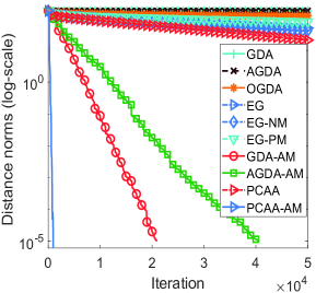
(a) $n=100$

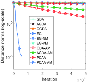
(b) $n=500$

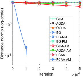
(c) $n=1000$

Figure 8: Comparison in terms of iteration on games $\min_{\theta}\max_{\phi}V(\theta,\phi)=\theta^{\mathrm{T}}A\phi+\theta^{\mathrm{T}}b+c^{\mathrm{T}}\phi$. Except for PCAA and PCAA-AM using parameters $\gamma=1,\alpha=0,\beta=1$ in subfigures (a) and (b), and using parameters $\alpha=0,\gamma=1,\beta=2$ in subfigure (c), the parameter settings for the other algorithms in these three experiments are the same as in [30, Figure 4].

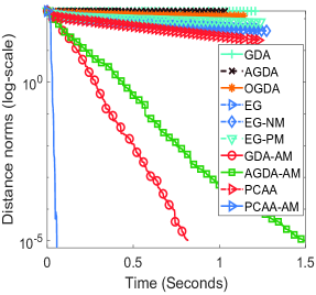
(a) $n=100$

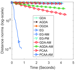
(b) $n=500$

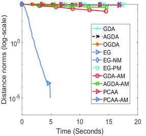
(c) $n=1000$

Figure 9: Comparison between methods in terms of time.

Above, we compared the numerical performance of ten algorithms when the matrix $A$ is a full-rank square matrix in bilinear game $\min_{\theta}\max_{\phi}V(\theta,\phi)=\theta^{\mathrm{T}}A\phi+\theta^{\mathrm{T}}b+c^{\mathrm{T}}\phi$. The results showed that combining PCAA with Anderson mixing is more effective for solving the game. Now, we continue to test the numerical performance of the ten algorithms on this bilinear game with matrix $A$ is not necessarily square. The experimental results are shown in Figure 10 and Figure 11. It should be noted that according to Proposition 3.1, the norm of the gradient of GDA iteration points increases continuously with the number of iterations. The experimental results in this example align with the theoretical analysis. However, plotting the graph of GDA together with the graphs of the other nine algorithms would obscure the differences in the latter. Therefore, in the following experiments, we did not include the norm graph of the GDA iteration points.

The experimental results in Figure 10 indicate that PCAA, without using Anderson mixing, achieves smaller norms of the gradients of the iteration points compared to AGDA, OGDA, EG, EG-NM and EG-PM. This suggests that PCAA converges faster than AGDA, OGDA, EG, EG-NM and EG-PM in this case. However, the results in Figure 11 show that PCAA takes relatively more time compared to the other five algorithms. When Anderson mixing is applied to GDA, AGD, and PCAA, we can compare the norms of the gradients of the iteration points of GDA-AM, AGDA-AM, and PCAA-AM, given the same number of iterations, based on the results presented in Figures 10 and 11. It can be observed that PCAA-AM has smaller norms of the gradients of the iteration points compared to GDA-AM and AGDA-AM. We would like to add that although the results on the graph may appear to overlap for AGDA-AM and PCAA-AM, in reality, the norm values of the gradients obtained by PCAA-AM are slightly smaller. However, as shown in the time comparison graph in Figure 11, PCAA-AM takes slightly more time compared to GDA-AM and AGDA-AM.

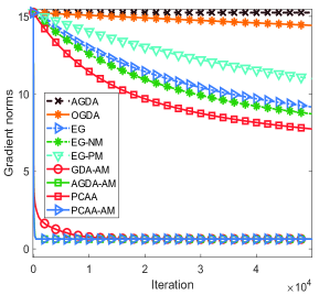
(a) $m=100,n=98$

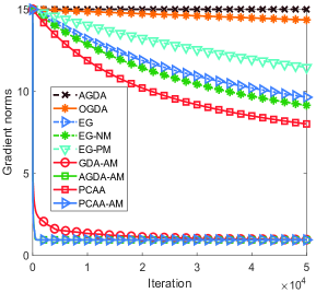
(b) $m=100,n=102$

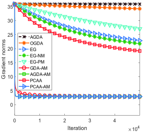
(c) $m=500,n=510$

Figure 10: Comparison in terms of iteration on games $\min_{\theta}\max_{\phi}V(\theta,\phi)=\theta^{\mathrm{T}}A\phi+\theta^{\mathrm{T}}b+c^{\mathrm{T}}\phi,A\in\mathbb{R}^{m\times n}$. Except for PCAA and PCAA-AM using parameters $\gamma=0.01,\alpha=0,\beta=0.01$ in subfigures (a),(b) and (c), the parameter settings for the other algorithms in these three experiments are are all set to $0.01$.

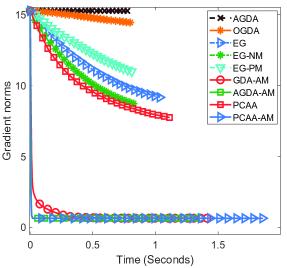
(a) $m=100,n=98$

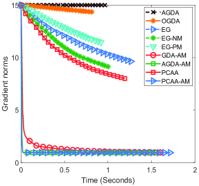
(b) $m=100,n=102$

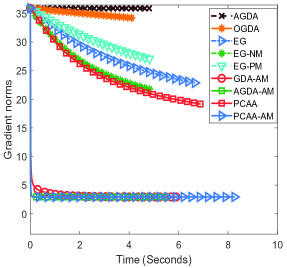
(c) $m=500,n=510$

Figure 11: Comparison between methods in terms of time.

7.2 Wasserstein GAN-GP on CelebA

It should be noted that after the proposal of Extra-Adam in [44], it was tested using GANs architecture on the CelebA dataset. The effectiveness of the proposed algorithm in training GANs was illustrated by showing improved FID (Fréchet inception distance) values compared to Adam. On the other hand, based on the analysis of the algorithm framework in subsection 6.2, does the empirical evidence support our theoretical analysis? In light of this, we conducted numerical experiments on the CelebA dataset to demonstrate the effectiveness of the algorithm. Additionally, through practical experiments, we aim to validate our theoretical analysis.

Experiment 1: Wasserstein GAN-GP on CelebA. Next, we trained Wasserstein GAN-GP using the proposed algorithm on the CelebA dataset to demonstrate the effectiveness of the algorithm, as evidenced by the FID scores. This serves as an answer to the aforementioned question two in subsection 6.2. The network architecture of the Wasserstein GAN is presented in Table 1, which has been trained on the CIFAR10 dataset for GANs training in [23]. The specific experimental setup can be found in Table 2, and the hyperparameter settings for the comparative algorithms are provided in Table 3.

Table 1: ResNet architecture used for our CelebA experiment

Generator

Input: $z\in\mathbb{R}^{128}\sim\mathcal{N}(0,I)$

Linear $128\rightarrow 128\times 4\times 4$

ResBlock  $128\rightarrow 128$

ResBlock  $128\rightarrow 128$

ResBlock  $128\rightarrow 128$

Batch Normalization

${\rm ReLU}(\cdot)$

conv. (kernel: $3\times 3,128\rightarrow 3$, stride: 1 , pad: 1 )

${\rm Tanh}(\cdot)$

Discriminator

Input: $x\in\mathbb{R}^{3\times 32\times 32}$

ResBlock  $~{}~{}~{}3\rightarrow 128$

ResBlock  $128\rightarrow 128$

ResBlock  $128\rightarrow 128$

ResBlock  $128\rightarrow 128$

Linear  $128\rightarrow 1$

Table 2: Experimental environment on the CelebA dataset

Experimental environment
CPU:	Inter Core i7-10700	GPU:	RTX A4000 16G
RAM:	64 G	Python:	Version 3.8.0
PyTorch:	Version 1.9.0

Table 3: (ResNet) WGAN-GP hyperparameters

Hyperparameters settings
Batch size	$64$
Max iterations T	$200,000$
Adam $\beta_{1}$	$0.5$
Adam $\beta_{2}$	$0.9$
Gradient penalty	$10$
GAN objective	Wasserstein GAN-GP
Learning rate for generator	$\gamma=2\times 10^{-5}$ (for Adam, Extra-Adam)
	$\gamma=\beta=2\times 10^{-5},\;\alpha=2.1\times 10^{-5}$ (for PCAA-Adam)
Learning rate for discriminator	$\gamma=2\times 10^{-5}$ (for Adam, Extra-Adam)
	$\gamma=\beta=2\times 10^{-5},\;\alpha=2.1\times 10^{-5}$ (for PCAA-Adam)

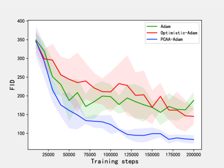
Figure 12: Mean and standard deviation of the FID computed over 5 runs for each method on Wasserstein GAN-GP trained on CelebA.

The comparison graph of FID values obtained during the training process using Adam, Extra-Adam, and PCAA-Adam algorithms shows that Wasserstein GAN-GP trained with PCAA-Adam consistently achieve smaller FID values in the middle to later stages of training. This not only demonstrates the effectiveness of the PCAA-Adam algorithm but also supports our analysis of the algorithm framework. Moreover, The results of Experiment 1 indicate that introducing the concept of centripetal acceleration to Adam can stabilize the training process and achieve smaller FID values. This suggests that the trained GANs have distributions that are closer to the real data distribution.

Experiment 2: Wasserstein GAN-GP with different network architectures on CelebA dataset. The purpose of this experiment is the same as experiment 1. The difference is that we have increased the number of pixels, making the differences in FID values more apparent through the clarity of the generated samples. The network architecture of the Wasserstein GAN is presented in Table 4, the specific experimental setup can be found in Table 2, and the hyperparameter settings for the comparative algorithms are provided in Table 5.

Table 4: ResNet architecture used for our CelebA experiment

Generator

Input: $z\in\mathbb{R}^{128}\sim\mathcal{N}(0,I)$

Linear $128\rightarrow 512\times 8\times 8$

ResBlock  $512\rightarrow 256$

ResBlock  $256\rightarrow 128$

ResBlock  $128\rightarrow 64$

Batch Normalization

${\rm ReLU}(\cdot)$

conv. (kernel: $3\times 3$, $64\rightarrow 3$, stride: 1 , pad: 1 )

${\rm Tanh}(\cdot)$

Discriminator

Input: $x\in\mathbb{R}^{3\times 64\times 64}$

ResBlock  $~{}~{}~{}3\rightarrow 128$

ResBlock  $128\rightarrow 128$

ResBlock  $128\rightarrow 256$

ResBlock  $256\rightarrow 512$

Linear  $512\rightarrow 1$

Table 5: (ResNet) WGAN-GP hyperparameters

Hyperparameters settings
Batch size	$64$
Max iterations T	$200,000$
Adam $\beta_{1}$	$0.0$
Adam $\beta_{2}$	$0.9$
Gradient penalty	$10$
GAN objective	Wasserstein GAN-GP
Learning rate for generator	$\gamma=2\times 10^{-4}$ (for Adam, Extra-Adam)
	$\gamma=\beta=2\times 10^{-4},\;\alpha=2.4\times 10^{-4}$ (for PCAA-Adam)
Learning rate for discriminator	$\gamma=2\times 10^{-4}$ (for Adam, Extra-Adam)
	$\gamma=\beta=2\times 10^{-4},\;\alpha=2.4\times 10^{-4}$ (for PCAA-Adam)

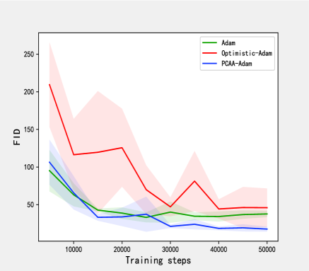
(a)

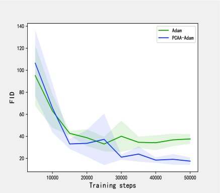
(b)

Figure 13: Mean and standard deviation of the FID computed over 5 runs for each method on Wasserstein GAN-GP trained on CelebA. (a): Comparison of FID values obtained from a single training process of Adam, Extra-Adam, and PCAA-Adam. (b): Comparison of FID values obtained from separate training processes of Adam and PCAA-Adam in the left figure. Due to the significant fluctuations in the FID values obtained from Extra-Adam in the left figure, it diminishes the visual effect of the FID values obtained from Adam and PCAA-Adam. Therefore, in the right figure, a separate comparison of the FID values obtained from the training processes of Adam and PCAA-Adam is presented.

(a) PCAA-Adam for CelebA

(b) Adam for CelebA

(c) Optimistic-Adam for CelebA

Figure 14: The figure shows a comparison of generated images by the generator at the end of training the Wasserstein GAN using Adam, Extra-Adam and PCAA-Adam.

The FID comparison graph Figure 13 reveals that after a fluctuation in the mid-training phase, the FID value obtained from Adam continues to increase, while the FID values obtained from Extra-Adam and PCAA-Adam initially increase and then rapidly decrease. This demonstrates that the introduction of the extra gradient technique and the centripetal acceleration idea can enhance the robustness of the FID values obtained during training. Comparing the FID values obtained from Extra-Adam and PCAA-Adam, it is observed that after the fluctuation, the FID value obtained from Extra-Adam exhibits a trend of increasing and then decreasing. However, the FID value obtained from PCAA-Adam continues to decrease. This indicates that the incorporation of the centripetal acceleration idea, which involves incorporating gradient-related information from the prediction step into the update step, can improve the practical performance of Extra-Adam. It also demonstrates the effectiveness of our algorithm. Figure 14 depicts a comparison of the generated images by the generator at the end of training for Adam, Extra-Adam, and PCAA-Adam. The smaller the FID value, the clearer the generated images. PCAA-Adam achieves the smallest FID value and generates the clearest images, thus visually demonstrating the effectiveness of the PCAA-Adam algorithm.

8 Conclusion

In response to the open problem of how to eliminate limit cycle behavior in zero-sum games using optimization techniques, as proposed in [31], and combining the research ideas of GANs training algorithms. This paper first demonstrated the fact that GDA does not converge on the general bilinear game through geometric and convergence rate analysis. Moreover, it proved that the limit point of PCAA iteration sequence was a Nash equilibrium point. Then, we obtained the last-iterate linear convergence rate of PCAA on the general bilinear game, which outperformed the results obtained in the comparative literature. Finally, we validated the effectiveness of our proposed PCAA-Adam algorithm for training GANs through practical experiments.

Nevertheless, training general GANs involves the use of optimization algorithms and deep learning frameworks to tackle a non-convex non-concave zero-sum game. The current research status in the international community reveals that both theoretical and algorithmic aspects of non-convex non-concave zero-sum games encompass various important and challenging problems that require attention [64]. Additionally, the stability of training processes for many GAN variants is highly intricate and represents an area for further investigation in our research. Furthermore, recently Chae et al. [12, 13] has shown that two-timescale EG holds the potential to address the open problem studied in their paper. However, their results do not yet guarantee that the limit points of the algorithm’s iterates are Local minimax optima. Therefore, they invite the academic community to propose new algorithms or more reasonable concepts of Local minimax optima to address the unresolved issues. Since PCAA can reduce to EG, can PCAA provide some insights into solving the open problem of their interest? And can PCAA almost surely avoid strict non-minimax points? These questions are all waiting to be further explored.

This work was supported by Major Program of National Natural Science Foundation of China (Nos. 11991020, 11991024).

References

• [1] Abernethy J, Lai K A, Wibisono A. Last-iterate convergence rates for min-max optimization: convergence of Hamiltonian gradient descent and consensus optimization. In: Proceedings of the 32nd International Conference on Algorithmic Learning Theory. Berlin: Springer, 2021, 3–47
• [2] Alawieh M B, Li W, Lin Y, et al. High-definition routing congestion prediction for large-scale FPGAs. In: 2020 25th Asia and South Pacific Design Automation Conference. New York: IEEE, 2020, 26–31
• [3] Anagnostides I, Penna P. Solving zero-sum games through alternating projections. ArXiv:2010.00109, 2020
• [4] Arjovsky M, Chintala S, Bottou L. Wasserstein generative adversarial networks. In: Proceedings of the 34th International Conference on Machine Learning. New York: ICML, 2017, 214–223
• [5] Azizian W, Mitliagkas I, Lacoste -Julien S, et al. A tight and unified analysis of gradient-based methods for a whole spectrum of differentiable games. In: Proceedings of the Twenty-Third International Conference on Artificial Intelligence and Statistics. New York: PMLR, 2020, 2863–2873
• [6] Bailey J P, Gidel G, Piliouras G. Finite regret and cycles with fixed step-size via alternating gradient descent-ascent. In: Proceedings of Thirty Third Annual Conference on Learning Theory. New York: PMLR, 2020, 391–407
• [7] Balduzzi D, Racaniere S, Martens J, et al. The mechanics of n-player differentiable games. In: Proceedings of the 35th International Conference on Machine Learning. New York: ICML, 2018, 354–363
• [8] Bao X C, Zhang G D. Finding and only finding local Nash equilibria by both pretending to be a follower. ICLR 2022 Workshop on Gamification and Multiagent Solutions. New Washington DC: ICLR, 2022
• [9] Berard H, Gidel G, Almahairi A, et al. A closer look at the optimization landscapes of generative adversarial networks. In: International Conference on Learning Representations. Washington DC: ICLR, 2020
• [10] Brock A, Donahue J, Simonyan K. Large scale GAN training for high fidelity natural image synthesis. In: International Conference on Learning Representations. Washington DC: ICLR, 2018
• [11] Cai S, Obukhov A, Dai D, et al. Pix2nerf: unsupervised conditional $\pi$-GAN for single image to neural radiance fields translation. In: computer vision and pattern recognition, New York: IEEE, 2022, 3981-3990.
• [12] Chae J, Kim K, Kim D. Open problem: is there a first-order method that only converges to local minimax optima. In: Proceedings of Thirty Sixth Annual Conference on Learning Theory. New York: PMLR, 2023, 5957-5964.
• [13] Chae J, Kim K, Kim D. Two-timescale Extragradient for Finding Local Minimax Points. ArXiv:2305.16242, 2023.
• [14] Chan E R, Lin C Z, Chan M A, et al. Efficient geometry-aware 3D generative adversarial networks. In: Computer Vision and Pattern Recognition, New York: IEEE, 2022, 16123-16133.
• [15] Chavdarova T, Pagliardini M, Jaggi M, et al. Taming GANs with lookahead-minmax. In: International Conference on Learning Representations. Washington DC: ICLR, 2021
• [16] Crowson K, Biderman S, Kornis D, et al. VQGAN-CLIP: open domain image generation and editing with natural language guidance. In: European Conference on Computer Vision. Cham: Springer Nature Switzerland. 2022, 13697: 88-105, doi:10.1007/978-3-031-19836-6_6.
• [17] Daskalakis C, Ilyas A, Syrgkanis V, et al. Training GANs with optimism. In: International Conference on Learning Representations. Washington DC: ICLR, 2018
• [18] Daskalakis C, Panageas I. Last-iterate convergence: zero-sum games and constrained min-max optimization. In: Innovations in Theoretical Computer Science conference. Wadern:Dagstuhl Publishing, 2019.
• [19] Daskalakis C, Panageas I. The limit points of (optimistic) gradient descent in min-max optimization. In: Advances in Neural Information Processing Systems 31. Cambridge: MIT Press, 2018, 9236–9246
• [20] Fang S, Han F, Liang W Y, et al. An improved conditional generative adversarial network for microarray data. In: International Conference on Intelligent Computing. Berlin: Springer, 2020, 105–114, doi:10.1007/978-3-030-60799-9_9
• [21] Razavi -Far R, Ruiz -Garcia A, Palade V, et al. Generative adversarial learning: architectures and applications. Cham: Springer, 2022.
• [22] Gidel G. Multi-player games in the era of machine learning. PhD Thesis. Montréal: Université de Montréal, 2021
• [23] Gidel G, Berard H, Vignoud G, et al. A variational inequality perspective on generative adversarial networks. In: International Conference on Learning Representations. Washington DC: ICLR, 2019
• [24] Gidel G, Hemmat R A, Pezeshki M, et al. Negative momentum for improved game dynamics. In: Proceedings of the Twenty-Second International Conference on Artificial Intelligence and Statistics. New York: PMLR, 2019, 1802–1811
• [25] Gidel G, Jebara T, Lacoste -Julien S. Frank-Wolfe algorithms for saddle point problems. In: Proceedings of the 20th International Conference on Artificial Intelligence and Statistics. New York: PMLR, 2017, 362–371
• [26] Goodfellow I. NIPS 2016 tutorial: generative adversarial networks. ArXiv:1701.00160, 2016
• [27] Goodfellow I, Pouget-Abadie J, Mirza M, et al. Generative adversarial nets. In: Advances in Neural Information Processing Systems 27. Cambridge: MIT Press, 2014, 2672–2680
• [28] Grnarova P, Kilcher Y, Levy K Y, et al. Generative minimization networks: training GANs without competition. ArXiv:2103.12685, 2021
• [29] He H, Zhao S F, Xi Y Z, et al. AGE: enhancing the convergence on GANs using alternating extra-gradient with gradient extrapolation. In: NeurIPS 2021 Workshop on Deep Generative Models and Downstream Applications. Cambridge: MIT Press, 2021
• [30] He H, Zhao S F, Xi Y Z, et al. Solve minimax optimization by Anderson acceleration. In: International Conference on Learning Representations. Washington DC: ICLR, 2022
• [31] Hsieh Y P. Convergence without convexity: sampling, optimization, and games. PhD Thesis. Lausanne: École Polytechnique Fédérale de Lausanne, 2020
• [32] Jesse E, Kumar K A, Shuo C, et al. GANSynth: adversarial neural audio synthesis, In: International Conference on Learning Representations. Washington DC: ICLR, 2019
• [33] Jin C, Netrapalli P, Jordan M I. What is local optimality in nonconvex-nonconcave minimax optimization. In: Proceedings of the 37th International Conference on Machine Learning. New York: ICML, 2020, 4880–4889
• [34] Kingma D P, Ba J. Adam: a method for stochastic optimization. ArXiv:1412.6980, 2014
• [35] Korpelevich G M. The extragradient method for finding saddle points and other problems, Matecon, 1976, 12:747–756,
• [36] Lei N, An D S, Guo Y, et al. A geometric understanding of deep learning. Engineering, 2020, 6: 361–374, doi:10.1016/j.eng.2019.09.010
• [37] Li K K, Yang X M, Zhang K. Training GANs with predictive centripetal acceleration (in Chinese). Sci China Math, 2023, doi:10.1360/SSM-2022-0237 (to appear)
• [38] Liang T Y, Stokes J. Interaction matters: a note on non-asymptotic local convergence of generative adversarial networks. In: Proceedings of the Twenty-Second International Conference on Artificial Intelligence and Statistics. New York: PMLR, 2019, 907–915
• [39] Lin T Y, Jin C, Jordan M I. On gradient descent ascent for nonconvex-concave minimax problems. In: Proceedings of the 37th International Conference on Machine Learning. New York: ICML, 2020, 6083–6093
• [40] Lorraine J, Acuna D, Vicol P, et al. Complex momentum for learning in games. ArXiv:2102.08431, 2021
• [41] Lv W, Xiong J, Shi J, et al. A deep convolution generative adversarial networks based fuzzing framework for industry control protocols. J Intell Manuf, 2021, 32: 441–457, doi:10.1007/s10845-020-01584-z
• [42] Mazumdar E V, Jordan M I, Sastry S S. On finding local Nash equilibria (and only local Nash equilibria) in zero-sum games. ArXiv:1901.00838, 2019.
• [43] Mertikopoulos P, Papadimitriou C, Piliouras G. Cycles in adversarial regularized learning. In: Proceedings of the Twenty-Ninth Annual ACM-SIAM Symposium on Discrete Algorithms. New York: ACM, 2018, 2703–2717, doi:10.1137/1.9781611975031.172
• [44] Mertikopoulos P, Zenati H, Lecouat B, et al. Optimistic mirror descent in saddle-point problems: going the extra (gradient) mile. In: International Conference on Learning Representations. Washington DC: ICLR, 2019
• [45] Mescheder L, Geiger A, Nowozin S. Which training methods for GANs do actually converge. In: Proceedings of the 35th International Conference on Machine Learning. New York: ICML, 2018, 3481–3490
• [46] Mescheder L, Nowozin S, Geiger A. The numerics of GANs. In: Advances in Neural Information Processing Systems 30. Cambridge: MIT Press, 2017, 1825–1835
• [47] Mishchenko K, Kovalev D, Shulgin E, et al. Revisiting stochastic extragradient. In: Proceedings of the Twenty Third International Conference on Artificial Intelligence and Statistics. New York: PMLR, 2020, 4573–4582
• [48] Mokhtari A, Ozdaglar A, Pattathil S. A unified analysis of extra-gradient and optimistic gradient methods for saddle point problems: Proximal point approach. In: Proceedings of the Twenty-Third International Conference on Artificial Intelligence and Statistics. New York: PMLR, 2020, 1497–1507
• [49] Nedić A, Ozdaglar A. Subgradient methods for saddle-point problems. J Optim Theory Appl, 2009, 142: 205–228, doi:10.1007/s10957-009-9522-7
• [50] Odena A. Open questions about generative adversarial networks. Distill, 2019, 4: e18, doi:10.23915/distill.00018
• [51] Ouyang Y Y, Xu Y Y. Lower complexity bounds of first-order methods for convex-concave bilinear saddle-point problems. Math Program, 2021, 185: 1–35, doi:10.1007/s10107-019-01420-0
• [52] Peng W, Dai Y H, Zhang H, et al. Training GANs with centripetal acceleration. Optim Methods Softw, 2020, 35: 1–19, doi:10.1080/10556788.2020.1754414
• [53] Pethick T, Latafat P, Patrinos P, et al. Escaping limit cycles: global convergence for constrained nonconvex-nonconcave minimax problems. ArXiv:2302.09831, 2023.
• [54] Pinetz T, Soukup D, Pock T. What is optimized in Wasserstein GANs. In: Proceedings of the 23rd Computer Vision Winter Workshop. New York: IEEE, 2018
• [55] Qu Y Y, Zhang J W, Li R D, et al. Generative adversarial networks enhanced location privacy in 5G networks. Sci China Inf Sci, 2020, 63: 1–12, doi:10.1007/s11432-019-2834-x
• [56] Radford A, Metz L, Chintala S. Unsupervised representation learning with deep convolutional generative adversarial networks. ArXiv:1511.06434, 2015
• [57] Ryu E K, Yuan K, Yin W T. ODE analysis of stochastic gradient methods with optimism and anchoring for minimax problems and GANs. ArXiv:1905.10899, 2019
• [58] Salimans T, Goodfellow I, Zaremba W, et al. Improved techniques for training GANs. In: Advances in Neural Information Processing Systems 29. Cambridge: MIT Press, 2016, 2234–2242
• [59] Saxena D, Cao J. Generative adversarial networks (GANs) challenges, solutions, and future directions. ACM Computing Surveys, 2021, 54: 1–42, doi:10.1145/3446374
• [60] Shen J Y, Chen X H, Heaton H, et al. Learning a minimax optimizer: a pilot study. In: International Conference on Learning Representations. Washington DC: ICLR, 2020
• [61] Skorokhodov I, Tulyakov S, Elhoseiny M. StyleGAN-V: a continuous video generator with the price, image quality and perks of StyleGAN2. In: Computer Vision and Pattern Recognition, New York: IEEE, 2022, 3626-3636.
• [62] Vondrick C, Pirsiavash H, Torralba A. Generating videos with scene dynamics. In: Advances in Neural Information Processing Systems 29. Cambridge: MIT Press, 2016, 613–621
• [63] Wang Y. A mathematical introduction to generative adversarial nets (GAN). ArXiv:2009.00169, 2020.
• [64] Xu Z, Zhang H L. Optimization algorithms and their complexity analysis for non-convex minimax problems (in Chinese). Operations Research Transactions, 2021, 25: 74–86, doi:10.15960/j.cnki.issn.1007-6093.2021.03.004
• [65] Yuan Y X, et al. Chinese Discipline Development Strategy$\bm{\cdot}$Mathematical Optimization (in Chinese). Beijing: Science Press, 2020
• [66] Zhang G J, Yu Y L. Convergence behaviour of some gradient-based methods on bilinear zero-sum games. In: International Conference on Learning Representations. Washington DC: ICLR, 2020
• [67] Zhang J Y, M Y Hong, S Z Zhang. On lower iteration complexity bounds for the convex concave saddle point problems. Math Program, 2022, 194: 901–935, doi:10.1007/s10107-021-01660-z
• [68] Zhang M, Lucas J, Ba J, et al. Lookahead optimizer: k steps forward, 1 step back. In: Advances in Neural Information Processing Systems 32. Cambridge: MIT Press, 2019, 9597–9608