A Simple and Efficient Tensor Calculus for Machine Learning

Abstract

Computing derivatives of tensor expressions, also known as tensor calculus, is a fundamental task in machine learning. A key concern is the efficiency of evaluating the expressions and their derivatives that hinges on the representation of these expressions. Recently, an algorithm for computing higher order derivatives of tensor expressions like Jacobians or Hessians has been introduced that is a few orders of magnitude faster than previous state-of-the-art approaches. Unfortunately, the approach is based on Ricci notation and hence cannot be incorporated into automatic differentiation frameworks from deep learning like TensorFlow, PyTorch, autograd, or JAX that use the simpler Einstein notation. This leaves two options, to either change the underlying tensor representation in these frameworks or to develop a new, provably correct algorithm based on Einstein notation. Obviously, the first option is impractical. Hence, we pursue the second option. Here, we show that using Ricci notation is not necessary for an efficient tensor calculus and develop an equally efficient method for the simpler Einstein notation. It turns out that turning to Einstein notation enables further improvements that lead to even better efficiency.

The methods that are described in this paper have been implemented in the online tool www.MatrixCalculus.org for computing derivatives of matrix and tensor expressions.

An extended abstract of this paper appeared as “A Simple and Efficient Tensor Calculus”, AAAI 2020 [1].

1 Introduction

Many problems in machine learning are naturally written in terms of tensor expressions. Any algorithmic method for computing derivatives of such expressions is called a tensor calculus. Standard automatic differentiation (deep learning) frameworks like TensorFlow [2], PyTorch [3], autograd [4], and JAX [5] are very efficient when computing derivatives of scalar-valued functions. However, evaluating the derivatives of non-scalar-valued functions, for instance, Jacobians or Hessians, in these frameworks is up to three orders of magnitude slower than evaluating the derivatives that are computed by the approach of Laue et al. [6].

There have been some recent attempts to alleviate this lack of efficiency by accelerating the underlying linear algebra using automatic batching and optimizing the computational graphs of the derivatives [7]. These improvements have been incorporated into TensorFlow and JAX. However, the improvements are rather small and the efficiency gap of up to three orders of magnitude still persists.

On the other hand, the approach of Laue et al. [6] relies crucially on Ricci notation and therefore cannot be incorporated into standard deep learning frameworks that use the simpler Einstein notation. Here, we remove this obstacle and provide an efficient tensor calculus in Einstein notation. Already the simple version of our approach is as efficient as the approach by Laue et al. [6]. We provide further improvements that lead to an even better efficiency.

Ricci notation distinguishes between co- and contravariant indices, that is, upper and lower indices. This distinction is necessary in order to compute derivatives in a mathematical correct way. Consider for instance the simple expression $x^{\top}Ax$. If we want to compute the derivative of this expression with respect to the vector $x$, then, at some point, we face the problem of computing the derivative of $x^{\top}$. However, this derivative in Ricci notation is the delta-tensor $\delta_{ij}$ that cannot be represented in linear algebra. Note, it is not the identity matrix which is represented in Ricci notation as $\delta^{i}_{j}$. Hence, in order to represent the derivative in a mathematical correct way, upper and lower indices are necessary. This problem has its roots in mathematical tensor analysis, where tensors are used for representing multilinear functions by their values on a set of basis vectors. These values are stored in a tensor, that is, a multi-dimensional array. Upper and lower indices are used to distinguish between vector space and dual vector space components that transform differently under basis changes. In the example expression, $x$ is a vector while $x^{\top}$ is a co-vector from the dual vector space.

In machine learning tensors are typically not used for representing multi-linear functions, but simply as multi-dimensional arrays for storing data and parameters. Hence, there is no need to distinguish different types of components. Indices can just be used for accessing the different tensor components. This is basically Einstein notation that is used in all deep learning frameworks.

The contribution of this paper is an efficient and coherent method for computing tensor derivatives in Einstein notation together with a correctness proof. In reverse mode automatic differentiation, our method is equivalent to the efficient approach in [6] for computing higher order derivatives. Additionally, we show that reverse mode is not optimal. A combination of reverse and forward mode, known as cross-country mode, can be more efficient. Efficiency can be further improved by compressing higher order derivatives.

For validating our framework we compute Hessians for several machine learning problems. It turns out that our method, because of the additional optimizations, outperforms the approach of [6] which is already a few orders of magnitude more efficient than TensorFlow, PyTorch, autograd, and JAX.

Related Work.

Many details on the fundamentals and more advanced topics of automatic differentiation can be found in the book by Griewank and Walther [8]. Baydin et al. [9] provide an excellent survey on automatic differentiation for machine learning.

Computing derivatives of non-scalar-valued functions is discussed in the work by Pearlmutter [10]. In this approach, if the function returns an $n$-dimensional vector, then its derivative is computed by treating each entry as a separate scalar-valued function. The same idea is employed in almost all implementations for computing derivatives of non-scalar-valued functions. Gebremedhin et al. [11] introduce some optimizations based on graph coloring algorithms.

Magnus and Neudecker [12] can compute derivatives with respect to vectors and matrices. At the core of their approach, matrices are turned into vectors by stacking columns of a matrix into one long vector. Then, the Kronecker matrix product is used to emulate higher order tensors. This approach works well for computing first order derivatives of scalar-valued functions. However, it is not practicable for computing higher order derivatives.

Giles [13] collects a number of derivatives for matrix operators, i.e., pushforward and pullback functions for automatic differentiation. Similarly, Seeger et al. [14] provide methods and code for computing derivatives of Cholesky factorizations, QR decompositions, and symmetric eigenvalue decompositions. However, they all require that the output function is scalar-valued, and hence, cannot be generalized to higher order derivatives.

Kakade and Lee [15] consider non-smooth functions and provide a provably correct algorithm that returns an element from the subdifferential. However, their algorithm is also restricted to scalar-valued functions.

Another line of research focuses on automatic differentiation from a programming language point of view. The goal is to incorporate gradient computations into programming languages with the goal of fully general differentiable programming [16]. Work towards this goal includes the Tangent package [17], the Myia project [18], and the approach of Fei et al. [19]. So far this work is again restricted to scalar-valued functions.

Recently, also second order information has been considered for training deep nets. For instance, this information can be exploited for escaping one of the many saddle points, but also for turning the final classifier more robust [20]. Furthermore, some differences in the convergence behavior can be explained by looking at the spectrum of the Hessian of the objective function [21, 22, 23]. However, so far it has been prohibitive to compute the full Hessian even for small networks. Here, in our experiments, we also compute the Hessian of a small neural net.

2 Einstein Notation

Table 1: Comparison of different linear algebra notations.

vectorized	Ricci	Einstein
$yx^{\top}$	$y^{i}x_{j}$	$y*_{(i,j,ij)}x$
$Ax$	$A^{i}_{j}x^{j}$	$A*_{(ij,j,i)}x$
$y^{\top}x$	$y_{i}x^{i}$	$y*_{(i,i,\emptyset)}x$
$AB$	$A^{i}_{j}B^{j}_{k}$	$A*_{(ij,jk,ik)}B$
$y\odot x$	$y^{i}x^{i}$	$y*_{(i,i,i)}x$
$A\odot B$	$A^{i}_{j}B^{i}_{j}$	$A*_{(ij,ij,ij)}B$
$A\cdot\operatorname{diag}(x)$	$A^{i}_{j}x^{i}$	$A*_{(ij,i,ij)}x$

In tensor calculus one distinguishes three types of multiplication, namely inner, outer, and element-wise multiplication. Indices are important for distinguishing between these types. For tensors $A,B,$ and $C$ any multiplication of $A$ and $B$ can be written as

$$C[s_{3}]=\sum_{(s_{1}\cup s_{2})\setminus s_{3}}A[s_{1}]\cdot B[s_{2}],$$

where $C$ is the result tensor and $s_{1},s_{2}$, and $s_{3}$ are the index sets of the left argument, the right argument, and the result tensor, respectively. The summation is only relevant for inner products that in Ricci calculus are denoted by shared upper and lower indices. If one does not want to distinguish between upper and lower indices, then the summation must be made explicit through the result tensor. The standard way to do so is by excluding the index for summation from the index set of the result tensor. Hence, the index set of the result tensor is always a subset of the union of the index sets of the multiplication’s arguments, that is, $s_{3}\subseteq(s_{1}\cup s_{2})$. In the following we denote the generic tensor multiplication simply as $C=A*_{(s_{1},s_{2},s_{3})}B$, where $s_{3}$ explicitly represents the index set of the result tensor. This notation is basically identical to the tensor multiplication einsum in NumPy, TensorFlow, and PyTorch, and to the notation used in the Tensor Comprehension Package [24].

The $*_{(s_{1},s_{2},s_{3})}$-notation comes close to standard Einstein notation. In Einstein notation the index set $s_{3}$ of the output is omitted and the convention is to sum over all shared indices in $s_{1}$ and $s_{2}$. This, however, restricts the types of multiplications that can be represented. The set of multiplications that can be represented in standard Einstein notation is a proper subset of the multiplications that can be represented by our notation. For instance, standard Einstein notation is not capable of representing element-wise multiplications directly. Still, in the following we refer to the $*_{(s_{1},s_{2},s_{3})}$-notation simply as Einstein notation as it is standard practice in all deep learning frameworks.

Table 1 shows examples of tensor expressions in standard linear algebra notation, Ricci calculus, and Einstein notation. The first group shows an outer product, the second group shows inner products, and the last group shows examples of element-wise multiplications. As can be seen in Table 1, Ricci notation and Einstein notation are syntactically reasonably similar. However, semantically they are quite different. As pointed out above, Ricci notation differentiates between co- and contravariant dimensions/indices and Einstein notation does not. While this might seem like a minor difference, it does have substantial implications when computing derivatives. For instance, when using Ricci notation, forward and reverse mode automatic differentiation can be treated in the same way [6]. This is no longer the case when using Einstein notation.

We can show that the generic tensor multiplication operator $*_{(s_{1},s_{2},s_{3})}$ is associative, commutative, and satisfies the distributive property. Our tensor calculus, that we introduce in the next section, makes use of all three properties. By $s_{1}s_{2}$ we denote the concatenation of the index sets $s_{1}$ and $s_{2}$. An example where the concatenation of two index sets is used is the outer product of two vectors, see e.g., the first row in Table 1.

Lemma 1 (Associativity).

Let $s_{1},s_{2},s_{3}$, and $s_{4}$ be index sets with $s_{3}\subseteq s_{1}\cup s_{2}$ and $s_{4}\cap(s_{1}\cup s_{2})=\emptyset$. Then it holds that

$$\left(A*_{(s_{1},s_{2}s_{4},s_{3}s_{4})}B\right)*_{(s_{3}s_{4},s_{4},s_{3})}C=A*_{(s_{1},s_{2},s_{3})}\left(B*_{(s_{2}s_{4},s_{4},s_{2})}C\right).$$

Proof.

We have

$$\left(A*_{(s_{1},s_{2}s_{4},s_{3}s_{4})}B\right)*_{(s_{3}s_{4},s_{4},s_{3})}C =\quad\sum_{s_{4}}\left(\sum_{(s_{1}\cup s_{2})\setminus s_{3}}A[s_{1}]\cdot B[s_{2}s_{4}]\right)\cdot C[s_{4}]$$

$$=\quad\sum_{\left((s_{1}\cup s_{2})\setminus s_{3}\right)\cup s_{4}}A[s_{1}]\cdot B[s_{2}s_{4}]\cdot C[s_{4}]$$

$$=\quad\sum_{(s_{1}\cup s_{2})\setminus s_{3}}A[s_{1}]\left(\sum_{s_{4}}B[s_{2}s_{4}]\cdot C[s_{4}]\right)$$

$$=\quad A*_{(s_{1},s_{2},s_{3})}\left(B*_{(s_{2}s_{4},s_{4},s_{2})}C\right)$$

∎

Unlike standard matrix multiplication tensor multiplication is commutative.

Lemma 2 (Commutativity).

It holds that

$$A*_{(s_{1},s_{2},s_{3})}B=B*_{(s_{2},s_{1},s_{3})}A.$$

Proof.

Follows immediately from our definition of the tensor multiplication operator $*_{(s_{1},s_{2},s_{3})}$, the commutativity of the scalar multiplication, and the commutativity of the set union operation. ∎

Lemma 3 (Distributive property).

Let $s_{1},s_{2}$, and $s_{3}$ be index sets with $s_{3}\subseteq s_{1}\cup s_{2}$. It holds that

$$A*_{(s_{1},s_{2},s_{3})}B+A*_{(s_{1},s_{2},s_{3})}C=A*_{(s_{1},s_{2},s_{3})}\left(B+C\right).$$

Proof.

Follows from the distributive property of the scalar multiplication. ∎

3 Tensor Calculus

Now we are prepared to develop our tensor calculus. We start by giving the definition of the derivative of a tensor-valued expression with respect to a tensor. For the definition, we use $\left\|A\right\|=\sqrt{\sum_{s}A[s]^{2}}$ as the norm of a tensor $A$ which coincides with the Euclidean norm if $A$ is a vector and with the Frobenius norm if $A$ is a matrix.

Definition 4 (Fréchet Derivative).

Let $f\colon\mathbb{R}^{n_{1}\times n_{2}\times\ldots\times n_{k}}\to\mathbb{R}^{m_{1}\times m_{2}\times\ldots\times m_{l}}$ be a function that takes an order-$k$ tensor as input and maps it to an order-$l$ tensor as output. Then, $D\in\mathbb{R}^{m_{1}\times m_{2}\times...\times m_{l}\times n_{1}\times n_{2}\times\ldots\times n_{k}}$ is called the derivative of $f$ at $x$ if and only if

$$\lim_{h\to 0}\frac{\left\|f(x+h)-f(x)-D\circ h\right\|}{\left\|h\right\|}=0,$$

where $\circ$ is an inner tensor product.

Here, the dot product notation $D\circ h$ is short for the inner product $D*_{(s_{1}s_{2},s_{2},s_{1})}h$, where $s_{1}s_{2}$ is the index set of $D$ and $s_{2}$ is the index set of $h$. For instance, if $D\in\mathbb{R}^{m_{1}\times n_{1}\times n_{2}}$ and $h\in\mathbb{R}^{n_{1}\times n_{2}}$, then $s_{1}=\{i,j,k\}$ and $s_{2}=\{j,k\}$.

In the following, we first describe forward and reverse mode automatic differentiation for expressions in Einstein notation, before we discuss extensions like cross-country mode and compression of higher order derivatives that are much easier to realize in Einstein than in Ricci notation. As can be seen from our experiments in Section 4, the extensions allow for significant performance gains.

3.1 Forward Mode

Any tensor expression has an associated directed acyclic expression graph (expression DAG). Figure 1 shows the expression DAG for the expression

$$X^{\top}(\exp(X\cdot w)+1)^{-1}\odot\exp(X\cdot w)),$$ (1)

where $\odot$ denotes the element-wise multiplication and ^-1 the element-wise multiplicative inverse.

Figure 1: Expression DAG for Expression (1)

The nodes of the DAG that have no incoming edges represent the variables of the expression and are referred to as input nodes. The nodes of the DAG that have no outgoing edges represent the functions that the DAG computes and are referred to as output nodes. Let the DAG have $n$ input nodes (variables) and $m$ output nodes (functions). We label the input nodes as $x_{0},...,x_{n-1}$, the output nodes as $y_{0},...,y_{m-1}$, and the internal nodes as $v_{0},\ldots,v_{k-1}$. Every internal and every output node represents either a unary or a binary operator. The arguments of these operators are supplied by the incoming edges.

In forward mode, for computing derivatives with respect to the input variable $x_{j}$, each node $v_{i}$ will eventually store the derivative $\frac{\partial v_{i}}{\partial x_{j}}$ which is traditionally denoted as $\dot{v}_{i}$. It is computed from input to output nodes as follows: At the input nodes that represent the variables $x_{i}$, the derivatives $\frac{\partial x_{i}}{\partial x_{j}}$ are stored. Hence, these are either unit tensors if $i=j$ or zero tensors otherwise. Then, the derivatives that are stored at the remaining nodes, here called $f$, are iteratively computed by summing over all their incoming edges as

$$\dot{f}=\frac{\partial f}{\partial x_{j}}=\sum_{z\,:\,(z,f)\in E}\frac{\partial f}{\partial z}\cdot\frac{\partial z}{\partial x_{j}}=\sum_{z\,:\,(z,f)\in E}\frac{\partial f}{\partial z}\cdot\dot{z},$$

where $\frac{\partial f}{\partial z}$ is the partial derivative of node $f$ with respect to $z$ and the multiplication is tensorial. The so called pushforwards $\dot{z}$ of the predecessor nodes $z$ of $f$ have been computed before and are stored at $z$. Hence, the derivative of each function is stored at the corresponding output node $y$ of the expression DAG. Obviously, the updates can be done simultaneously for one input variable $x_{j}$ and all output nodes $y_{i}$. Computing the derivatives with respect to all input variables requires $n$ such rounds.

In the following, we derive the explicit form of the pushforward for nodes of the expression DAG of a tensor expression. For such a DAG we can distinguish four types of nodes, namely multiplication nodes, general unary function nodes, element-wise unary function nodes, and addition nodes. General unary functions are general tensor-valued functions while element-wise unary functions are applied to each entry of a single tensor. The difference can be best explained by the difference between the matrix exponential function (general unary function) and the ordinary exponential function applied to every entry of the matrix (element-wise unary function). The pushforward for addition nodes is trivially just the sum of the pushforward of the two summands. Thus, it only remains to show how to compute the pushforward for multiplication, general unary functions, and element-wise unary function nodes.

Theorem 5.

Let $x$ be an input variable with index set $s_{4}$ and let $C=A*_{(s_{1},s_{2},s_{3})}B$ be a multiplication node of the expression DAG. The pushforward of $C$ is

$$\dot{C}=B*_{(s_{2},s_{1}s_{4},s_{3}s_{4})}\dot{A}+A*_{(s_{1},s_{2}s_{4},s_{3}s_{4})}\dot{B}.$$

Proof.

By the definition of the forward mode the pushforward $\dot{C}$ is given as

$$\dot{C}=\frac{\partial C}{\partial A}\cdot\dot{A}+\frac{\partial C}{\partial B}\cdot\dot{B}.$$

We show first how to compute $\frac{\partial C}{\partial B}\cdot\dot{B}$. According to Definition 4 it holds that

$$\lim_{h\to 0}\frac{1}{\left\|h\right\|}\cdot\left\|B(x+h)-B(x)-\dot{B}\circ h\right\|=0.$$

We have the following sequence of equalities

$$C(x+h)- C(x)-\dot{C}\circ h$$

$$=A*_{(s_{1},s_{2},s_{3})}B(x+h)-A*_{(s_{1},s_{2},s_{3})}B(x)-\left(A*_{(s_{1},s_{2}s_{4},s_{3}s_{4})}\dot{B}\right)\circ h$$

$$=A*_{(s_{1},s_{2},s_{3})}B(x+h)-A*_{(s_{1},s_{2},s_{3})}B(x)-\left(A*_{(s_{1},s_{2}s_{4},s_{3}s_{4})}\dot{B}\right)*_{(s_{3}s_{4},s_{4},s_{3})}h$$

$$=A*_{(s_{1},s_{2},s_{3})}B(x+h)-A*_{(s_{1},s_{2},s_{3})}B(x)-A*_{(s_{1},s_{2},s_{3})}\left(\dot{B}*_{(s_{2}s_{4},s_{4},s_{2})}h\right)$$

$$=A*_{(s_{1},s_{2},s_{3})}\left(B(x+h)-B(x)-\dot{B}*_{(s_{2}s_{4},s_{4},s_{2})}h\right)$$

$$=A*_{(s_{1},s_{2},s_{3})}\left(B(x+h)-B(x)-\dot{B}\circ h\right).$$

The first equality follows from the definition of $\dot{C}$, the second from the definition of $\circ$, the third from Lemma 1, the fourth from Lemma 3, and the last from the definition of $\circ$. Thus, we have

$$\lim_{h\to 0}\frac{1}{\left\|h\right\|}\cdot\left\|C(x+h)-C(x)-\dot{C}\circ h\right\| =\lim_{h\to 0}\frac{1}{\left\|h\right\|}\cdot\left\|A*_{(s_{1},s_{2},s_{3})}\left(B(x+h)-B(x)-\dot{B}\circ h\right)\right\|$$

$$\leq\left\|A\right\|\lim_{h\to 0}\frac{1}{\left\|h\right\|}\cdot\left\|B(x+h)-B(x)-\dot{B}\circ h\right\|$$

$$=0$$

Hence, we get $\frac{\partial C}{\partial B}\cdot\dot{B}=A*_{(s_{1},s_{2}s_{4},s_{3}s_{4})}\dot{B}$. Similarly, we get that $\frac{\partial C}{\partial A}\cdot\dot{A}=B*_{(s_{2},s_{1}s_{4},s_{3}s_{4})}\dot{A}$. Combining the two equalities finishes the proof. ∎

Theorem 6.

Let $x$ be an input variable with index set $s_{3}$, let $f$ be a general unary function whose domain has index set $s_{1}$ and whose range has index set $s_{2}$, let $A$ be a node in the expression DAG, and let $C=f(A)$. The pushforward of the node $C$ is $\dot{C}=f^{\prime}(A)*_{(s_{2}s_{1},s_{1}s_{3},s_{2}s_{3})}\dot{A}$, where $f^{\prime}$ is the derivative of $f$.

Proof.

By Definition 4 we have

$$\lim_{\tilde{h}\to 0}\frac{1}{\left\|\tilde{h}\right\|}\cdot\left\|f(A+\tilde{h})-f(A)-f^{\prime}(A)\circ\tilde{h}\right\|=0.$$

Let $\tilde{h}=A(x+h)-A(x)$. Since $A$ is differentiable, we have that $\tilde{h}\to 0$ as $h\to 0$. Furthermore, we have that $\left\|A(x+h)-A(x)\right\|\leq 1/c\left\|h\right\|$ for some suitable constant $c$. Hence, we get

$$0 =\lim_{h\to 0}\frac{1}{\left\|A(x+h)-A(x)\right\|}\cdot\left\|f(A(x+h))-f(A)-f^{\prime}(A)\circ\left(A(x+h)-A(x)\right)\right\|$$

$$\geq\lim_{h\to 0}\frac{c}{\left\|h\right\|}\cdot\left\|f(A(x+h))-f(A)-f^{\prime}(A)\circ\left(A(x+h)-A(x)\right)\right\|$$ (2)

By Definition 4 we also have that

$$\lim_{h\to 0}\frac{1}{\left\|h\right\|}\cdot\left\|A(x+h)-A(x)-\dot{A}\circ h\right\|=0.$$

Hence, we can replace in the limit $A(x+h)-A(x)$ with $\dot{A}\circ h$ in (2) and obtain

$$0\geq\lim_{h\to 0}\frac{c}{\left\|h\right\|}\cdot\left\|f(A(x+h))-f(A)-f^{\prime}(A)\circ(\dot{A}\circ h)\right\|.$$

Note, that

$$f^{\prime}(A)\circ(\dot{A}\circ h) =f^{\prime}(A(x))\circ(\dot{A}*_{(s_{1}s_{3},s_{3},s_{1})}h)$$

$$=f^{\prime}(A(x))*_{(s_{2}s_{1},s_{1},s_{2})}(\dot{A}*_{(s_{1}s_{3},s_{3},s_{1})}h)$$

$$=(f^{\prime}(A(x))*_{(s_{2}s_{1},s_{1}s_{3},s_{2}s_{3})}\dot{A})*_{(s_{2}s_{3},s_{3},s_{2})}h)$$

$$=(f^{\prime}(A(x))*_{(s_{2}s_{1},s_{1}s_{3},s_{2}s_{3})}\dot{A})\circ h)$$

Hence, we obtain

$$0\geq\lim_{h\to 0}\frac{c}{\left\|h\right\|}\cdot\left\|f(A(x+h))-f(A)-(f^{\prime}(A(x))*_{(s_{2}s_{1},s_{1}s_{3},s_{2}s_{3})}\dot{A})\circ h)\right\|.$$

Thus, we get $\dot{C}=f^{\prime}(A)*_{(s_{2}s_{1},s_{1}s_{3},s_{2}s_{3})}\dot{A}$ as claimed. ∎

In case that the general unary function is simply an element-wise unary function that is applied element-wise to a tensor, Theorem 6 simplifies as follows.

Theorem 7.

Let $x$ be an input variable with index set $s_{2}$, let $f$ be an element-wise unary function, let $A$ be a node in the expression DAG with index set $s_{1}$, and let $C=f(A)$ where $f$ is applied element-wise. The pushforward of the node $C$ is $\dot{C}=f^{\prime}(A)*_{(s_{1},s_{1}s_{2},s_{1}s_{2})}\dot{A}$, where $f^{\prime}$ is the derivative of $f$.

Proof.

By Definition 4 we have

$$\lim_{h\to 0}\frac{1}{\left\|h\right\|}\cdot\left\|A(x+h)-A(x)-\dot{A}\circ h\right\|=0.$$

It follows that for every scalar tensor entry $A(x)_{s}$, where $s$ is the multi-index of the entry, that

$$\lim_{h\to 0}\frac{1}{\left\|h\right\|}\cdot\big{|}A(x+h)_{s}-A(x)_{s}-(\dot{A}\circ h)_{s}\big{|}=0.$$

Let $f^{h}(A,x)=f(A(x+h)-f(A(x))$. Since, $f$ is applied entrywise and $f^{\prime}$ is the derivative of $f$ we get from the chain rule for the scalar case that

$$\lim_{h\to 0}\frac{1}{\left\|h\right\|}\cdot\big{|}f^{h}(A,x)_{s}-f^{\prime}(A(x)_{s})\cdot(\dot{A}\circ h)_{s}\big{|}=0.$$

Since this equality holds for all multi-indices $s$ we get by summing over these indices that

$$\lim_{h\to 0}\frac{1}{\left\|h\right\|}\cdot\left\|f^{h}(A,x)-f^{\prime}(A(x))*_{(s_{1},s_{1},s_{1})}(\dot{A}\circ h)\right\|=0.$$

We have

$$f^{\prime}(A(x))*_{(s_{1},s_{1},s_{1})}(\dot{A}\circ h) =f^{\prime}(A(x))*_{(s_{1},s_{1},s_{1})}(\dot{A}*_{(s_{1}s_{2},s_{2},s_{1})}h)$$

$$=(f^{\prime}(A(x))*_{(s_{1},s_{1}s_{2},s_{1}s_{2})}\dot{A})*_{(s_{1}s_{2},s_{2},s_{1})}h$$

$$=(f^{\prime}(A(x))*_{(s_{1},s_{1}s_{2},s_{1}s_{2})}\dot{A})\circ h,$$

where the first and the last equality follow from the definition of $\circ$, and the second equality follows from Lemma 1. Hence, we have

$$\lim_{h\to 0}\bigg{(}\frac{1}{\left\|h\right\|}\cdot\Big{\|}f(A(x+h))-f(A(x))-(f^{\prime}(A(x))*_{(s_{1},s_{1}s_{2},s_{1}s_{2})}\dot{A})\circ h)\Big{\|}\bigg{)}=0.$$

Thus, we get $\dot{C}=f^{\prime}(A)*_{(s_{1},s_{1}s_{2},s_{1}s_{2})}\dot{A}$. ∎

3.2 Reverse Mode

Reverse mode automatic differentiation proceeds similarly to the forward mode, but from output to input nodes. Each node $v_{i}$ will eventually store the derivative $\frac{\partial y_{j}}{\partial v_{i}}$ which is usually denoted as $\bar{v}_{i}$, where $y_{j}$ is the function to be differentiated. These derivatives are computed as follows: First, the derivatives $\frac{\partial y_{j}}{\partial y_{i}}$ are stored at the output nodes of the DAG. Hence again, these are either unit tensors if $i=j$ or zero tensors otherwise. Then, the derivatives that are stored at the remaining nodes, here called $z$, are iteratively computed by summing over all their outgoing edges as follows

$$\bar{z}=\frac{\partial y_{j}}{\partial z}=\sum_{f\,:\,(z,f)\in E}\frac{\partial y_{j}}{\partial f}\cdot\frac{\partial f}{\partial z}=\sum_{f\,:\,(z,f)\in E}\bar{f}\cdot\frac{\partial f}{\partial z},$$

where the multiplication is again tensorial. The so-called pullbacks $\bar{f}$ have been computed before and are stored at the successor nodes $f$ of $z$. This means the derivatives of the function $y_{j}$ with respect to all the variables $x_{i}$ are stored at the corresponding input nodes of the expression DAG. Computing the derivatives for all the output functions requires $m$ such rounds.

In the following we describe the contribution of unary and binary operator nodes to the pullback of their arguments. We have only two types of binary operators, namely tensor addition and tensor multiplication. In the addition case the contribution of $C$ to the pullback of both of its arguments is simply $\bar{C}$. In Theorem 8 we derive the explicit form of the contribution of a multiplication node to the pullback of its arguments, in Theorem 9 the contribution of a general unary function, and in Theorem 10 we derive the contribution of an element-wise unary function node to its argument.

Theorem 8.

Let $Y$ be an output node with index set $s_{4}$ and let $C=A*_{(s_{1},s_{2},s_{3})}B$ be a multiplication node of the expression DAG. Then the contribution of $C$ to the pullback $\bar{B}$ of $B$ is $\bar{C}*_{(s_{4}s_{3},s_{1},s_{4}s_{2})}A$ and its contribution to the pullback $\bar{A}$ of $A$ is $\bar{C}*_{(s_{4}s_{3},s_{2},s_{4}s_{1})}B$.

Proof.

Here we only derive the contribution of $C$ to the pullback $\bar{B}$. Its contribution to $\bar{A}$ can be computed analogously. The contribution of $C$ to $\bar{B}$ is $\bar{C}\cdot\frac{\partial C}{\partial B}$. By Definition 4 we have for the derivative $\bar{C}=\frac{\partial Y}{\partial C}$ of $Y$ with respect to $C$ that

$$\lim_{\tilde{h}\to 0}\,\frac{1}{\|\tilde{h}\|}\cdot\Big{\|}Y(C+\tilde{h})-Y(C)-\bar{C}\circ\tilde{h}\Big{\|}=0.$$

By specializing $\tilde{h}=A*_{(s_{1},s_{2},s_{3})}h$ we get

$$Y(C+ \tilde{h})-Y(C)-\bar{C}\circ\tilde{h}$$

$$=Y(A*_{(s_{1},s_{2},s_{3})}B+A*_{(s_{1},s_{2},s_{3})}h)-Y(A*_{(s_{1},s_{2},s_{3})}B)-\bar{C}\circ(A*_{(s_{1},s_{2},s_{3})}h)$$

$$=Y(A*_{(s_{1},s_{2},s_{3})}(B+h))-Y(A*_{(s_{1},s_{2},s_{3})}B)-\bar{C}\circ(A*_{(s_{1},s_{2},s_{3})}h)$$

$$=Y(A*_{(s_{1},s_{2},s_{3})}(B+h))-Y(A*_{(s_{1},s_{2},s_{3})}B)-\bar{C}*_{(s_{4}s_{3},s_{3},s_{4})}(A*_{(s_{1},s_{2},s_{3})}h)$$

$$=Y(A*_{(s_{1},s_{2},s_{3})}(B+h))-Y(A*_{(s_{1},s_{2},s_{3})}B)-(\bar{C}*_{(s_{4}s_{3},s_{1},s_{4}s_{2})}A)*_{(s_{4}s_{2},s_{2},s_{4})}h)$$

$$=Y(A*_{(s_{1},s_{2},s_{3})}(B+h))-Y(A*_{(s_{1},s_{2},s_{3})}B)-(\bar{C}*_{(s_{4}s_{3},s_{1},s_{4}s_{2})}A)\circ h),$$

where the first equality follows from the definitions of $C$ and $\tilde{h}$, the second from Lemma 3, the third from the definition of $\circ$, the fourth from Lemma 1, the fifth from Lemma 2, and the last again from the definition of $\circ$. Hence, we have for $\frac{\partial Y}{\partial C}\cdot\frac{\partial C}{\partial B}$ that

$$0 =\lim_{\tilde{h}\to 0}\frac{1}{\big{\|}\tilde{h}\big{\|}}\cdot\left\|Y(C+\tilde{h})-Y(C)-\bar{C}\circ\tilde{h}\right\|$$

$$=\lim_{h\to 0}\frac{1}{\left\|h\right\|}\cdot\Big{\|}Y(A*_{(s_{1},s_{2},s_{3})}(B+h))-Y(A*_{(s_{1},s_{2},s_{3})}B)-(\bar{C}*_{(s_{4}s_{3},s_{1},s_{4}s_{2})}A)\circ h)\Big{\|}$$

Thus, the contribution of $C$ to the pullback $\bar{B}$ is

$$\frac{\partial Y}{\partial C}\cdot\frac{\partial C}{\partial B}=\bar{C}\cdot\frac{\partial C}{\partial B}=\bar{C}*_{(s_{4}s_{3},s_{1},s_{4}s_{2})}A.$$

∎

If the output function $Y$ in Theorem 8 is scalar-valued, then we have $s_{4}=\emptyset$ and the pullback function coincides with the function implemented in all modern deep learning frameworks including TensorFlow and PyTorch. Hence, our approach can be seen as a direct generalization of the scalar case.

Theorem 9.

Let $Y$ be an output function with index set $s_{3}$, let $f$ be a general unary function whose domain has index set $s_{1}$ and whose range has index set $s_{2}$, let $A$ be a node in the expression DAG, and let $C=f(A)$. The contribution of the node $C$ to the pullback $\bar{A}$ is

$$\bar{f}*_{(s_{3}s_{2},s_{2}s_{1},s_{3}s_{1})}f^{\prime}(A),$$

where $f^{\prime}$ is the derivative of $f$.

Proof.

The contribution of the node $C$ to the pullback $\bar{A}$ is $\bar{f}\cdot\frac{\partial f}{\partial A}$. By Definition 4 we have for the derivative $\bar{f}=\frac{\partial Y}{\partial f}$ of $Y$ with respect to $f$ that

$$\lim_{\tilde{h}\to 0}\frac{1}{\big{\|}\tilde{h}\big{\|}}\cdot\left\|Y(f+\tilde{h})-Y(f)-\bar{f}\circ\tilde{h}\right\|=0.$$ (3)

By specializing $\tilde{h}=f(A+h)-f(A)$ and setting $f=f(A)$ we get

$$Y(f+\tilde{h})-Y(f)-\bar{f}\circ\tilde{h}$$

$$\qquad\qquad\qquad=\,Y(f(A+h)-f(A)+f(A))-Y(f(A))-\bar{f}(A)\circ(f(A+h)-f(A))$$

$$\qquad\qquad\qquad=\,Y(f(A+h))-Y(f(A))-\bar{f}(A)\circ(f(A+h)-f(A))$$

Furthermore, since $f^{\prime}$ is the derivative of $f$ we have

$$\lim_{h\to 0}\frac{1}{\left\|h\right\|}\cdot\left\|\tilde{h}-f^{\prime}(A)*_{(s_{2}s_{1},s_{1},s_{2})}h\right\|=0.$$ (4)

Combining Equations (3) and (4) gives

$$0 =\lim_{\tilde{h}\to 0}\frac{1}{{\big{\|}\tilde{h}\big{\|}}}\cdot\left\|Y(f+\tilde{h})-Y(f)-\bar{f}\circ\tilde{h}\right\|$$

$$=\lim_{h\to 0}\frac{1}{\left\|h\right\|}\cdot\Big{\|}Y(f(A+h))-Y(f(A))-\bar{f}(A)\circ(f^{\prime}(A)*_{(s_{2}s_{1},s_{1},s_{2})}h)\Big{\|}$$

$$=\lim_{h\to 0}\frac{1}{\left\|h\right\|}\cdot\Big{\|}Y(f(A+h))-Y(f(A))-\bar{f}(A)*_{(s_{3}s_{2},s_{2},s_{3})}(f^{\prime}(A)*_{(s_{2}s_{1},s_{1},s_{2})}h)\Big{\|}$$

$$=\lim_{h\to 0}\frac{1}{\left\|h\right\|}\cdot\Big{\|}Y(f(A+h))-Y(f(A))-(\bar{f}(A)*_{(s_{3}s_{2},s_{2}s_{1},s_{3}s_{1})}f^{\prime}(A))*_{(s_{3}s_{1},s_{1},s_{3})}h\Big{\|}$$

$$=\lim_{h\to 0}\frac{1}{\left\|h\right\|}\cdot\Big{\|}Y(f(A+h))-Y(f(A))-(\bar{f}(A)*_{(s_{3}s_{2},s_{2}s_{1},s_{3}s_{1})}f^{\prime}(A))\circ h\Big{\|}$$

Hence, the contribution of the node $C$ to the pullback $\bar{A}$ is

$$\frac{\partial Y}{\partial f}\cdot\frac{\partial f}{\partial A}=\bar{f}\cdot\frac{\partial f}{\partial A}=\bar{f}*_{(s_{3}s_{2},s_{2}s_{1},s_{3}s_{1})}f^{\prime}(A).$$

∎

In case that the general unary function is simply an element-wise unary function that is applied element-wise to a tensor, Theorem 9 simplifies as follows.

Theorem 10.

Let $Y$ be an output function with index set $s_{2}$, let $f$ be an element-wise unary function, let $A$ be a node in the expression DAG with index set $s_{1}$, and let $C=f(A)$ where $f$ where $f$ is applied element-wise. The contribution of the node $C$ to the pullback $\bar{A}$ is

$$\bar{f}*_{(s_{2}s_{1},s_{1},s_{2}s_{1})}f^{\prime}(A),$$

where $f^{\prime}$ is the derivative of $f$.

Proof.

The contribution of the node $C$ to the pullback $\bar{A}$ is $\bar{f}\cdot\frac{\partial f}{\partial A}$. By Definition 4 we have for the derivative $\bar{f}=\frac{\partial Y}{\partial f}$ of $Y$ with respect to $f$ that

$$\lim_{\tilde{h}\to 0}\frac{1}{\big{\|}\tilde{h}\big{\|}}\cdot\left\|Y(f+\tilde{h})-Y(f)-\bar{f}\circ\tilde{h}\right\|=0.$$ (5)

By specializing $\tilde{h}=f(A+h)-f(A)$ and setting $f=f(A)$ we get

$$Y(f+\tilde{h})-Y(f)-\bar{f}\circ\tilde{h}$$

$$\qquad\qquad\qquad=\,Y(f(A+h)-f(A)+f(A))-Y(f(A))-\bar{f}(A)\circ(f(A+h)-f(A))$$

$$\qquad\qquad\qquad=\,Y(f(A+h))-Y(f(A))-\bar{f}(A)\circ(f(A+h)-f(A))$$

Furthermore, since $f^{\prime}$ is the derivative of $f$ and $f$ is an entrywise function we have

$$\lim_{h\to 0}\frac{1}{\left\|h\right\|}\cdot\left\|\tilde{h}-f^{\prime}(A)*_{(s_{1},s_{1},s_{1})}h\right\|=0.$$ (6)

Combining Equations (5) and (6) gives

$$0 =\lim_{\tilde{h}\to 0}\frac{1}{{\big{\|}\tilde{h}\big{\|}}}\cdot\left\|Y(f+\tilde{h})-Y(f)-\bar{f}\circ\tilde{h}\right\|$$

$$=\lim_{h\to 0}\frac{1}{\left\|h\right\|}\cdot\Big{\|}Y(f(A+h))-Y(f(A))-\bar{f}(A)\circ(f^{\prime}(A)*_{(s_{1},s_{1},s_{1})}h)\Big{\|}$$

$$=\lim_{h\to 0}\frac{1}{\left\|h\right\|}\cdot\Big{\|}Y(f(A+h))-Y(f(A))-\bar{f}(A)*_{(s_{2}s_{1},s_{1},s_{2})}(f^{\prime}(A)*_{(s_{1},s_{1},s_{1})}h)\Big{\|}$$

$$=\lim_{h\to 0}\frac{1}{\left\|h\right\|}\cdot\Big{\|}Y(f(A+h))-Y(f(A))-(\bar{f}(A)*_{(s_{2}s_{1},s_{1},s_{2}s_{1})}f^{\prime}(A))*_{(s_{2}s_{1},s_{1},s_{2})}h\Big{\|}$$

$$=\lim_{h\to 0}\frac{1}{\left\|h\right\|}\cdot\Big{\|}Y(f(A+h))-Y(f(A))-(\bar{f}(A)*_{(s_{2}s_{1},s_{1},s_{2}s_{1})}f^{\prime}(A))\circ h\Big{\|}$$

Hence, the contribution of the node $C$ to the pullback $\bar{A}$ is

$$\frac{\partial Y}{\partial f}\cdot\frac{\partial f}{\partial A}=\bar{f}\cdot\frac{\partial f}{\partial A}=\bar{f}*_{(s_{2}s_{1},s_{1},s_{2}s_{1})}f^{\prime}(A).$$

∎

3.3 Beyond Forward and Reverse Mode

Since the derivative of a function $y$ with respect to an input variable $x$ is the sum over all partial derivatives along all paths from $x$ to $y$, see e.g., [8], we can combine forward and reverse mode. Using that $\bar{v}=\frac{\partial y}{\partial v}$ and $\dot{v}=\frac{\partial v}{\partial x}$, we get

$$\frac{\partial y}{\partial x}=\sum_{v\in S}\bar{v}*_{(s_{1}s_{v},s_{v}s_{2},s_{1}s_{2})}\dot{v},$$

where $s_{v}$ is the index set of node $v$, $s_{1}$ is the index set of the output function $y$, $s_{2}$ is the index set of the input node $x$, and $S$ is the set of nodes in a cut of the expression DAG. General combinations of forward and reverse mode lead to the so-called cross-country mode. We will show that the differentiation of tensor expressions becomes even more efficient by a special instantiation of the cross-country mode and by compressing higher order derivatives.

Cross-Country Mode.

In both forward and reverse mode, derivatives are computed as sums of products of partial derivatives. In general, the time for evaluating the derivatives depends on the order by which the partial derivatives are multiplied. The two modes multiply the partial derivatives in opposite order. Derivatives are multiplied from input to output nodes in forward mode and vice versa in reverse mode.

If the output function is scalar-valued, then reverse mode is efficient for computing the derivative with respect to all input variables. It is guaranteed that evaluating the derivative takes at most six times the time for evaluating the function itself. In practice, usually a factor of two is observed [8]. However, this is no longer true for non-scalar-valued functions. In the latter case, the order of multiplying the partial derivatives has a strong impact on the evaluation time, even for simple functions, see e.g., Naumann [25]. Reordering the multiplication order of the partial derivatives is known as cross-country mode in the automatic differentiation literature [26]. Finding an optimal ordering is NP-hard [27] in general.

However, it turns out that significant performance gains for derivatives of tensor expressions can be obtained by the re-ordering strategy that multiplies tensors in order of their tensor-order, that is, multiplying vectors first, then matrices, and so on. We illustrate this strategy on the following example

$$f(x)=B\cdot g(h(Ax)),$$ (7)

where $A$ and $B$ are two matrices, $x$ is a vector and $g(.)$ and $h(.)$ are vector-valued functions that also take a vector as input. The derivative in this case is $B\operatorname{diag}(u)\operatorname{diag}(v)A$, where $u=g^{\prime}(h(Ax)),\,v=h^{\prime}(Ax)$, and $\operatorname{diag}(u)$ is the diagonal matrix with $u$ on its diagonal. Reverse mode multiplies these matrices from left to right while forward mode multiplies them from right to left. However, it is more efficient to first multiply the two vectors $u$ and $v$ element-wise and then to multiply the result with the matrices $A$ and $B$.

Actually, the structure of Example 7 is not contrived, but fairly common in second order derivatives. For instance, consider the expression $\sum g(h(Ax))$, where $g$ and $h$ are as above and the sum is over the vector components of the vector-valued expression $g(h(Ax))$. Many machine learning problems feature such an expression as subexpression, where $A$ is a data matrix and the optimization variable $x$ is a parameter vector. The gradient of this expression has the form of Example 7 with $B=A^{\top}$. As can be seen in the experiments in Section 4, reordering the multiplications by our strategy reduces the time for evaluating the Hessian by about $30\%$.

Compressing Derivatives.

Our compression scheme builds on the re-ordering scheme (cross-country mode) from above and on the simple observation that in forward as well as in reverse mode the first partial derivative is always a unit tensor. It is either, in reverse mode, the derivative of the output nodes with respect to themselves or, in forward mode, the derivative of the input nodes with respect to themselves. This unit tensor can always be moved to the end of the multiplications, if the order of multiplication is chosen exactly as in our cross-country mode strategy that orders the tensors in increasing tensor-order. Then, the multiplication with the unit tensor at the end is either trivial, i.e., amounts to a multiplication with a unit matrix that has no effect and thus can be removed, or leads to a compactification of the derivative.

For an example, consider the loss function

$$f(U)=\left\|T-UV^{\top}\right\|^{2}$$

of the non-regularized matrix factorization problem which is often used for recommender systems [28]. Here, $T\in\mathbb{R}^{n\times n},\,U,V\in\mathbb{R}^{n\times k}$ and $n$ is usually large while $k$ is small. The Hessian of $f$ is the fourth order tensor

$$H=2(V*_{(ij,ik,jk)}V)*_{(jl,ik,ijkl)}\mathbb{I}\in\mathbb{R}^{n\times k\times n\times k},$$

where $\mathbb{I}$ is the identity matrix. Newton-type algorithms for this problem solve the Newton system which takes time in $O\left((nk)^{3}\right)$. However, the Hessian can be compressed to $2(V*_{(ij,ik,jk)}V)$ which is a small matrix of size $k\times k$. This matrix can be inverted in $O(k^{3})$ time. The performance gain realized by compression can be significant. For instance, solving the compressed Newton system needs only about $10~{}\mu$sec whereas solving the original system needs about $1$ sec for a problem of size $n=1000$ and $k=10$. For more experimental results please refer to Section 4.

As another example, consider a simple neural net with a fixed number of fully connected layers, ReLU activation functions, and a softmax cross-entropy output layer. The Hessian of each layer is a fourth order tensor that can be written as $A*_{(ijl,ik,ijkl)}\mathbb{I}$ for a suitable third order tensor $A$. In this case, the Hessian can be compressed from a fourth order tensor to a third order tensor. For illustrative purposes, we provide expression trees for both derivatives, compressed and uncompressed, in the appendix. Computing with the compact representation of the Hessian is of course more efficient which we confirm experimentally in the next section.

4 Experiments

We have implemented both modes of the tensor calculus from the previous section together with the improvements that can be achieved by cross-country mode and the compactification of higher order derivatives. State-of-the-art frameworks like TensorFlow and PyTorch only support reverse mode since it allows to compute derivatives with respect to all input variables at the same time. Similarly to all other frameworks, our implementation performs some expression simplification like constant folding and removal of zero and identity tensors.

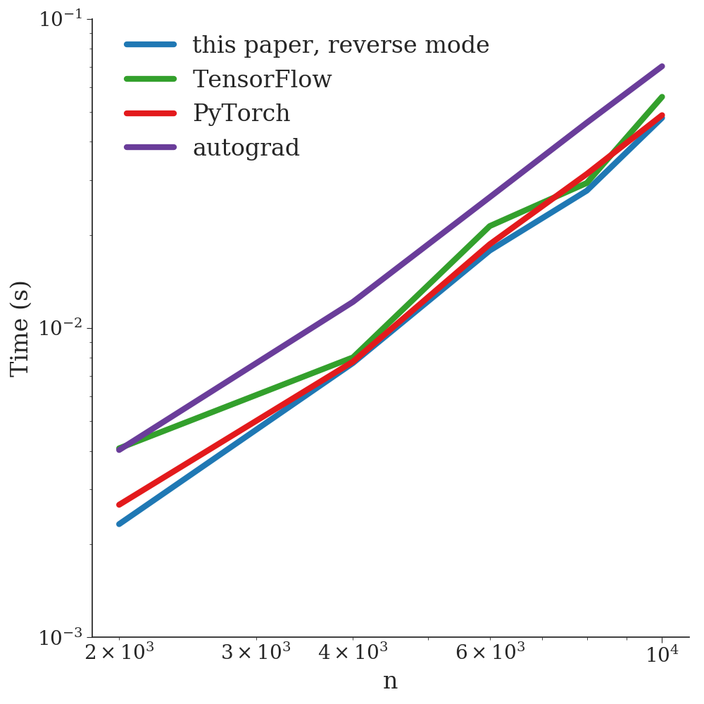
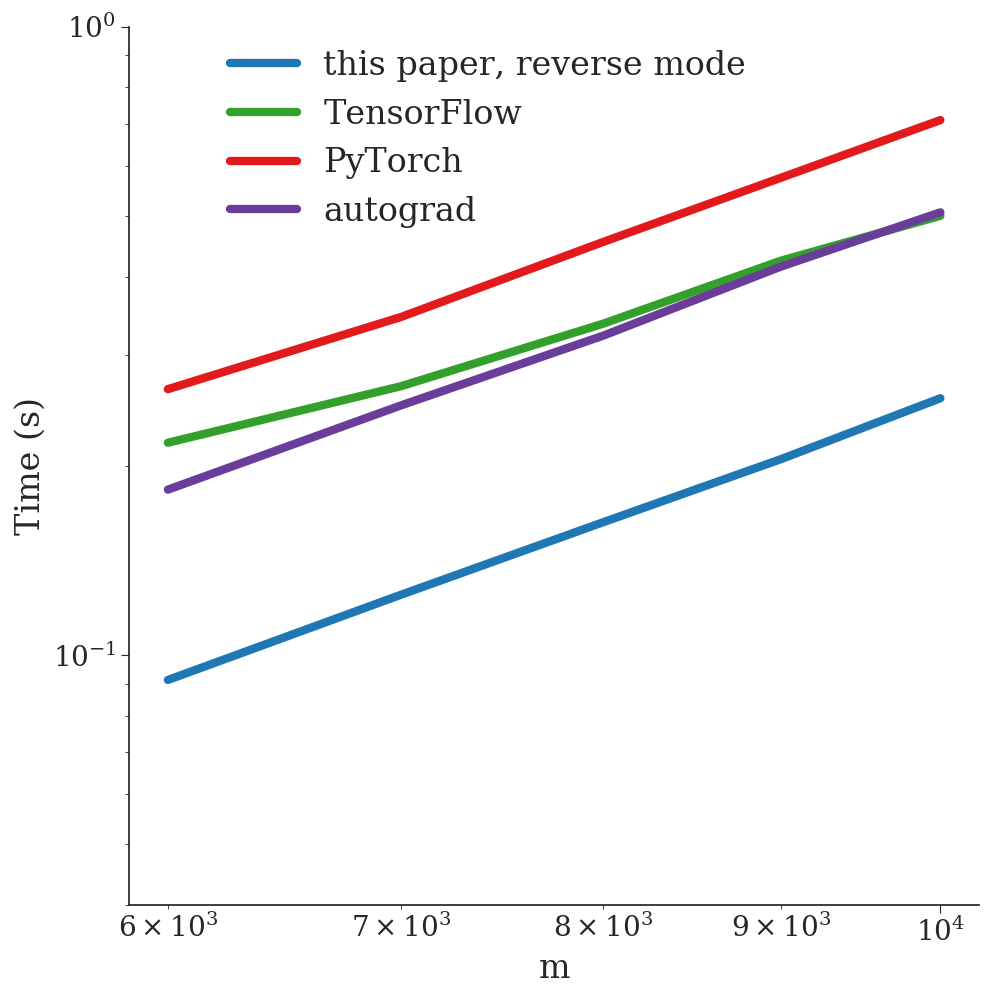
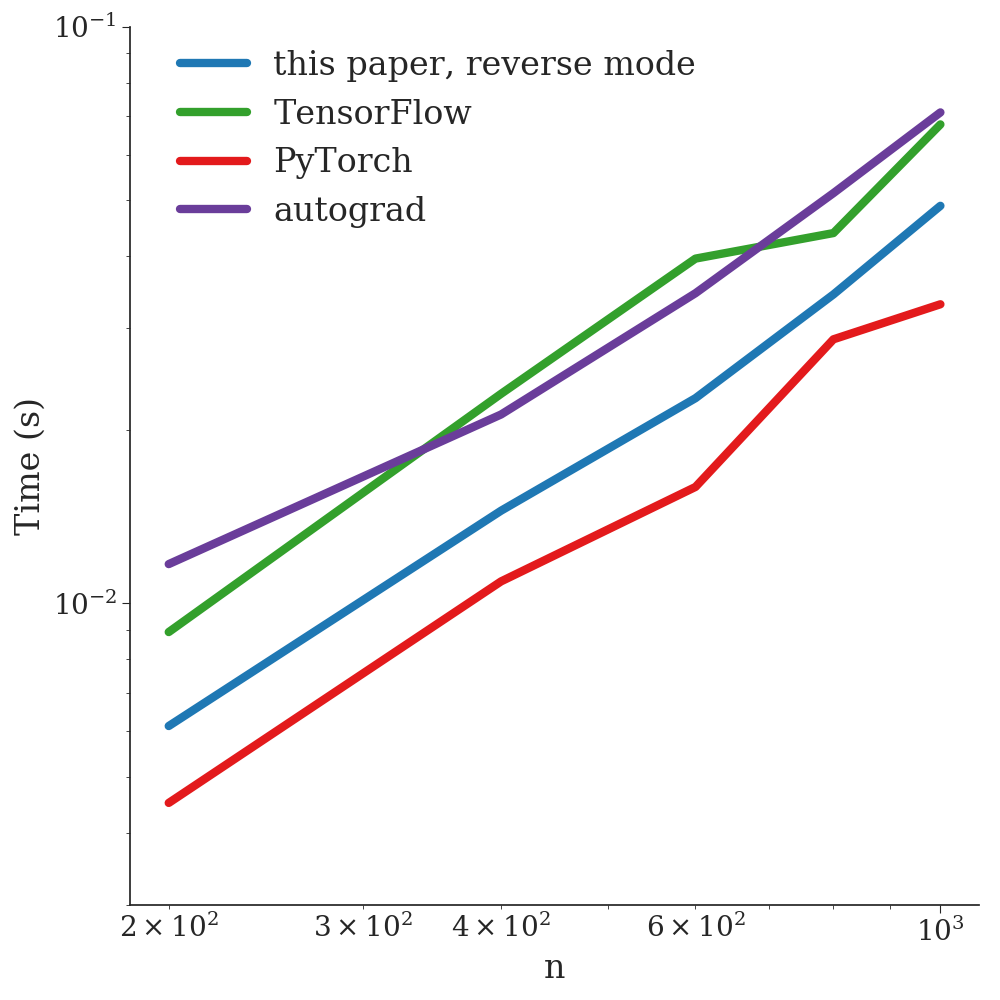
Figure 2: Running times for computing function value and gradient for the logistic regression function (left), matrix factorization (middle), and a small neural net (right). The times were measured on a CPU.

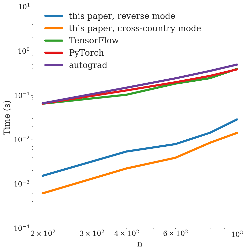
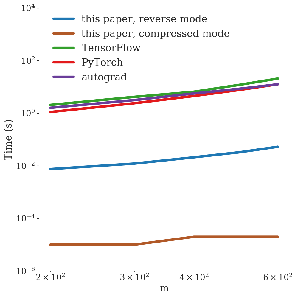
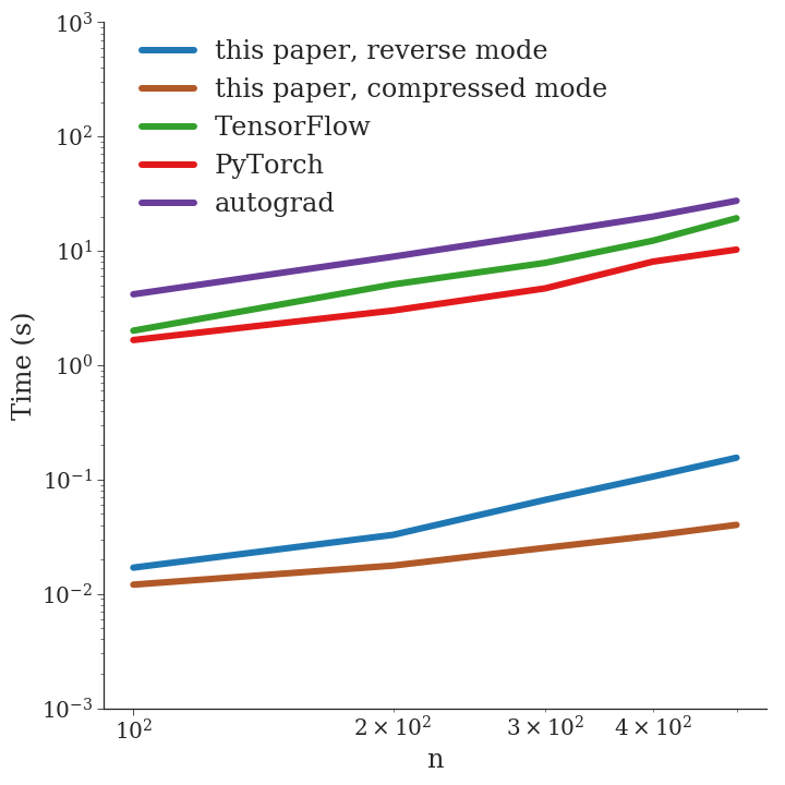
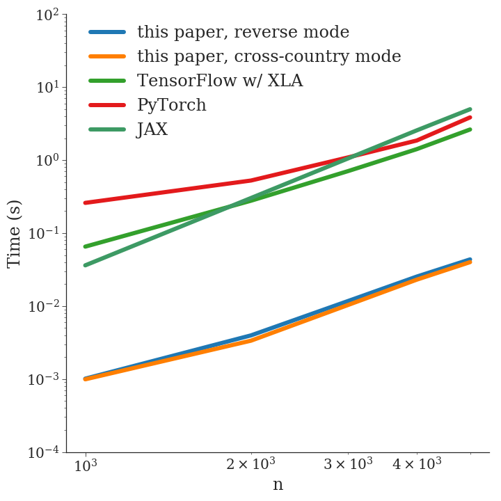
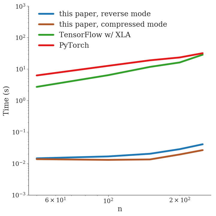
Figure 3: Running times on a CPU (top row) and on a GPU (bottom row) for computing the Hessian of the logistic regression function (left), matrix factorization (middle), and a small neural net (right).

Experimental Setup.

We followed the experimental setup of Laue et al. [6]. However, we added one more experiment, a small neural net. We have implemented our algorithms in Python. To evaluate expressions we used NumPy 1.16 and CuPy 5.1. We compared our framework with the state-of-the-art automatic differentiation frameworks that natively support linear algebra operations TensorFlow 1.14, PyTorch 1.0, autograd 1.2, and JAX 0.1.27 used with Python 3.6 that were all linked against the Intel MKL. All these frameworks support reverse mode automatic differentiation for computing first order derivatives. For scalar-valued functions the reverse mode of each of these frameworks coincides with the reverse mode of our approach. For non-scalar-valued functions all the frameworks compute the derivative for each entry of the output function separately. The expression DAGs that are generated by our reverse mode for general tensor expressions coincide with the derivatives computed by the approach presented in [6]. The experiments were run in a pure CPU setting (Intel Xeon E5-2643, 8 cores) as well as in a pure GPU setting (NVIDIA Tesla V100), except for autograd that does not provide GPU support.

We computed function values, gradients, and Hessians for each set of experiments. We computed Hessians on the CPU as well as on the GPU. To avoid the issue of sparsity patterns we generated dense, random data for each experiment. In this setting the running time does not depend on whether the data are synthetic or real world.

Logistic regression.

Logistic regression [29] is probably one of the most commonly used methods for classification. Given a set of $m$ data points $X\in\mathbb{R}^{m\times n}$ along with a set of binary labels $y\in\{\pm 1\}^{m}$, logistic regression aims at minimizing the loss function $\sum_{i}\log\left(\exp\left(-y^{(i)}\,(X^{(i)}w)\right)+1\right)$, where $w\in\mathbb{R}^{n}$ is the weight vector, $X^{(i)}$ is the $i$-th data point ($i$-th row of $X$), and $y^{(i)}$ the corresponding $i$-th label. The data matrix $X$ can be composed of the true input features, features transformed by basis functions/kernels [30, 31], or by random basis functions [32], or by features that have been learned by a deep net [33]. We set $m=2n$ in the experiments.

Matrix factorization.

Matrix factorization can be stated as the problem $\min_{U,V}\|T-UV^{\top}\|_{\Omega}^{2}$, where $T\in\mathbb{R}^{m\times n}$ is some target matrix, $U\in\mathbb{R}^{m\times k}$ and $V\in\mathbb{R}^{n\times k}$ are the low-rank factor matrices, and $\Omega\in\{0,1\}^{m\times n}$ is an indicator matrix that defines which elements of $T$ are known. Matrix factorization is mainly used in the context of recommender systems [28] or natural language processing [34, 35]. For the experiments, we set $k=5$ and compute the gradient and Hessian with respect to $U$. Note that the Hessian is a fourth order tensor.

Neural Net.

We have created a small neural net with ten fully connected layers, ReLU activation functions, and a softmax cross-entropy output layer. The weight matrices for the different layers all had the same size, $n\times n$. Here, we report running times for computing the Hessian of the first layer. Note, that the ReLU activation function, i.e., $f(x)=\max\{0,x\}$ is non-differential at $x=0$. All automatic differentiation packages return a subgradient in this case. However, it has been shown recently [36] that this convention still guarantees correctness in a generalized sense.

Evaluation.

In the case of scalar-valued functions all frameworks basically work in the same way. Thus, it is not surprising that their running times for computing function values and gradients are almost the same, see Figure 2.

The situation is different for Hessians. First, it can be seen that the reverse mode in our approach, whose results agree with the results in [6], is a few orders of magnitude faster than current state-of-the-art frameworks like TensorFlow, PyTorch, autograd, and JAX. This holds true for all experiments on the CPU and on the GPU, see Figure 3. For the logistic regression problem our cross-country mode is about $30\%$ faster on the CPU, while its effect on the GPU is negligible because of the GPU overhead. The performance gain of our compression scheme can be seen on the matrix factorization problem and on the neural net (middle and right column of Figure 3). Computing Hessians for small neural nets has now become feasible.

In our experiments, the effect of recent efforts in speeding up deep learning frameworks turned out to be rather small. Actually, enabling XLA for TensorFlow on the CPU slowed the computation down by a factor of two. Hence, we omit these running times in Figure 3. Enabling XLA on the GPU provided only marginal improvements. JAX which relies on XLA did not finish computations but raised memory errors indicating that it went out of main memory. These errors seem to be caused by the automatic batching function vmap that is used by JAX for auto-vectorization when computing Hessians. This was surprising to us since JAX is meant to be more memory efficient than TensorFlow. There is one exception, on the GPU, JAX finished the computation for the logistic regression problem. However, as can be seen in Figure 3, even in this case it is not significantly more efficient than the other deep learning frameworks. This was to be expected since JAX relies on XLA and the authors of XLA report a speed-up of only $15\%$ in the GPU setting [37].

5 Conclusion

We have developed a simple, efficient and provably correct framework for computing derivatives of general tensor expressions that is much simpler than previous approaches. Furthermore, it can be easily integrated into state-of-the-art frameworks like TensorFlow and PyTorch that use the same tensor representation, but are a few orders of magnitude slower than our approach when computing higher order derivatives. We have also demonstrated that reverse mode automatic differentiation is not optimal for computing higher order derivatives. Significant speed ups can be achieved by a special instantiation of the cross-country mode and by compressing higher order derivatives. The algorithms presented here form the basis for the online tool www.MatrixCalculus.org [38, 39] for computing derivatives of matrix and tensor expressions. It is also used within the GENO framework [40] for automatically generating optimization solvers from a given mathematical formulation. It can be accessed at www.geno-project.org [41].

Appendix

For illustration purposes, Figure 4 shows the computational graph of the Hessian of a net with three fully connected layers each with a ReLU activation function and a final cross-entropy layer that has been computed using reverse mode. Nodes that represent fourth order tensors are marked in red. Figure 4 shows that is impossible to eliminate these nodes easily when using reverse mode. Most of the computation time is actually spend in evaluating these fourth order tensors. However, using our instantiation of the cross-country mode it becomes possible to compute the Hessian without ever creating a fourth order tensor. See Figure 5 for the resulting computational graph. The only node that represents a fourth order tensor can now be safely removed as described in Section 3.3 of the main paper.

[Figures 4 and 5 follow on the next two pages]

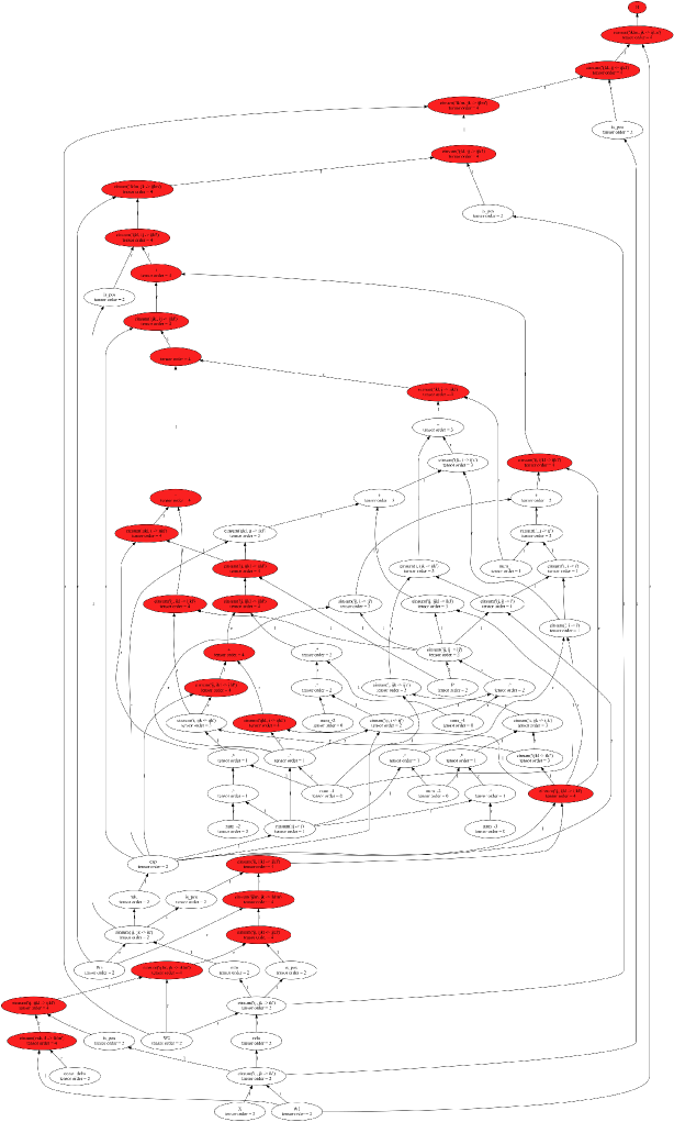
Figure 4: Hessian of a net with three fully connected layers, ReLU activation functions, and a cross-entropy layer when computed in reverse mode. Fourth order tensors are marked in red. Please note, the purpose of this figure is to illustrate that it is a non-trivial task to remove the fourth order tensor nodes when using reverse mode.

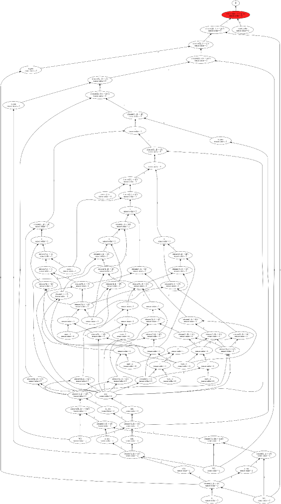
Figure 5: Hessian of a net with three fully connected layers, ReLU activation functions, and a cross-entropy layer when computed in our cross-country mode. The only node that represents a fourth order tensor, shown in red, can be easily removed due to using the cross-country mode.

References

- [1] Laue S, Mitterreiter M, Giesen J. A Simple and Efficient Tensor Calculus. In: Conference on Artificial Intelligence, (AAAI). 2020 .
- [2] Abadi M, et al. TensorFlow: A System for Large-scale Machine Learning. In: USENIX Conference on Operating Systems Design and Implementation (OSDI). USENIX Association. ISBN 978-1-931971-33-1, 2016 pp. 265–283.
- [3] Paszke A, Gross S, Chintala S, Chanan G, Yang E, DeVito Z, Lin Z, Desmaison A, Antiga L, Lerer A. Automatic differentiation in PyTorch. In: NIPS Autodiff workshop. 2017 .
- [4] Maclaurin D, Duvenaud D, Adams RP. Autograd: Effortless gradients in numpy. In: ICML AutoML workshop. 2015 .
- [5] Frostig R, Johnson MJ, Leary C. Compiling Machine Learning Programs via High-level Tracing. In: Conference on Systems and Machine Learning (SysML). 2018.
- [6] Laue S, Mitterreiter M, Giesen J. Computing Higher Order Derivatives of Matrix and Tensor Expressions. In: Advances in Neural Information Processing Systems (NeurIPS). 2018.
- [7] XLA and TensorFlow teams. XLA — TensorFlow, compiled. https://developers.googleblog.com/2017/03/xla-tensorflow-compiled.html, 2017.
- [8] Griewank A, Walther A. Evaluating derivatives - principles and techniques of algorithmic differentiation (2. ed.). SIAM, 2008.
- [9] Baydin AG, Pearlmutter BA, Radul AA, Siskind JM. Automatic Differentiation in Machine Learning: a Survey. Journal of Machine Learning Research, 2018. 18(153):1–43.
- [10] Pearlmutter BA. Fast Exact Multiplication by the Hessian. Neural Computation, 1994. 6(1):147–160.
- [11] Gebremedhin AH, Tarafdar A, Pothen A, Walther A. Efficient Computation of Sparse Hessians Using Coloring and Automatic Differentiation. INFORMS Journal on Computing, 2009. 21(2):209–223.
- [12] Magnus JR, Neudecker H. Matrix Differential Calculus with Applications in Statistics and Econometrics. John Wiley and Sons, third edition, 2007.
- [13] Giles MB. Collected Matrix Derivative Results for Forward and Reverse Mode Algorithmic Differentiation. In: Advances in Automatic Differentiation. Springer Berlin Heidelberg, 2008 pp. 35–44.
- [14] Seeger MW, Hetzel A, Dai Z, Lawrence ND. Auto-Differentiating Linear Algebra. In: NIPS Autodiff workshop. 2017 .
- [15] Kakade SM, Lee JD. Provably Correct Automatic Sub-Differentiation for Qualified Programs. In: Advances in Neural Information Processing Systems (NeurIPS), pp. 7125–7135. 2018.
- [16] LeCun Y. Deep Learning est mort. Vive Differentiable Programming! https://www.facebook.com/yann.lecun/posts/10155003011462143.
- [17] van Merriënboer B, Moldovan D, Wiltschko A. Tangent: Automatic differentiation using source-code transformation for dynamically typed array programming. In: Advances in Neural Information Processing Systems (NeurIPS). 2018.
- [18] van Merriënboer B, Breuleux O, Bergeron A, Lamblin P. Automatic differentiation in ML: Where we are and where we should be going. In: Advances in Neural Information Processing Systems (NeurIPS). 2018.
- [19] Wang F, Decker J, Wu X, Essertel G, Rompf T. Backpropagation with Callbacks: Foundations for Efficient and Expressive Differentiable Programming. In: Advances in Neural Information Processing Systems (NeurIPS). 2018.
- [20] Dey P, Nag K, Pal T, Pal NR. Regularizing Multilayer Perceptron for Robustness. IEEE Trans. Systems, Man, and Cybernetics: Systems, 2018. 48(8):1255–1266.
- [21] Ghorbani B, Krishnan S, Xiao Y. An Investigation into Neural Net Optimization via Hessian Eigenvalue Density. In: International Conference on Machine Learning (ICML). 2019.
- [22] Sagun L, Evci U, Güney VU, Dauphin Y, Bottou L. Empirical Analysis of the Hessian of Over-Parametrized Neural Networks. In: ICLR (Workshop). 2018 .
- [23] Yao Z, Gholami A, Keutzer K, Mahoney MW. Hessian-based Analysis of Large Batch Training and Robustness to Adversaries. In: Advances in Neural Information Processing Systems (NeurIPS). 2018 .
- [24] Vasilache N, Zinenko O, Theodoridis T, Goyal P, DeVito Z, Moses WS, Verdoolaege S, Adams A, Cohen A. Tensor Comprehensions: Framework-Agnostic High-Performance Machine Learning Abstractions. arXiv preprint arXiv:1802.04730, 2018.
- [25] Naumann U. Optimal accumulation of Jacobian matrices by elimination methods on the dual computational graph. Math. Program., 2004. 99(3):399–421.
- [26] Bischof CH, Hovland PD, Norris B. Implementation of automatic differentiation tools. In: ACM SIGPLAN Notices, volume 37. ACM, 2002 pp. 98–107.
- [27] Naumann U. Optimal Jacobian accumulation is NP-complete. Math. Program., 2008. 112(2):427–441.
- [28] Koren Y, Bell R, Volinsky C. Matrix Factorization Techniques for Recommender Systems. Computer, 2009. 42(8):30–37.
- [29] Cox DR. The Regression Analysis of Binary Sequences. Journal of the Royal Statistical Society. Series B (Methodological), 1958. 20(2):215–242.
- [30] Broomhead D, Lowe D. Multivariable Functional Interpolation and Adaptive Networks. Complex Systems, 1988. 2:321–355.
- [31] Schölkopf B, Smola AJ. Learning with Kernels: support vector machines, regularization, optimization, and beyond. Adaptive computation and machine learning series. MIT Press, 2002.
- [32] Rahimi A, Recht B. Random Features for Large-Scale Kernel Machines. In: Advances in Neural Information Processing Systems (NIPS). 2007 pp. 1177–1184.
- [33] Hinton GE, Osindero S, Teh YW. A Fast Learning Algorithm for Deep Belief Nets. Neural Computation, 2006. 18(7):1527–1554.
- [34] Blei DM, Ng AY, Jordan MI. Latent Dirichlet Allocation. Journal of Machine Learning Research, 2003. 3:993–1022.
- [35] Hofmann T. Probabilistic Latent Semantic Analysis. In: Conference on Uncertainty in Artificial Intelligence (UAI). 1999 pp. 289–296.
- [36] Lee W, Yu H, Rival X, Yang H. On Correctness of Automatic Differentiation for Non-Differentiable Functions. arXiv e-prints, 2020. abs/2006.06903.
- [37] XLA: Optimizing Compiler for TensorFlow. https://www.tensorflow.org/xla, 2019.
- [38] Laue S, Mitterreiter M, Giesen J. MatrixCalculus.org - Computing Derivatives of Matrix and Tensor Expressions. In: European Conference on Machine Learning and Principles and Practice in Knowledge Discovery in Databases (ECML-PKDD). 2019 pp. 769–772.
- [39] Laue S. On the Equivalence of Forward Mode Automatic Differentiation and Symbolic Differentiation. arXiv e-prints, 2019. abs/1904.02990.
- [40] Laue S, Mitterreiter M, Giesen J. GENO – GENeric Optimization for Classical Machine Learning. In: Advances in Neural Information Processing Systems (NeurIPS). 2019 .
- [41] Laue S, Mitterreiter M, Giesen J. GENO - Optimization for Classical Machine Learning Made Fast and Easy. In: Conference on Artificial Intelligence (AAAI). 2020 .
- [42] Theano Development Team. Theano: A Python framework for fast computation of mathematical expressions. arXiv e-prints, 2016. abs/1605.02688.
- [43] Rumelhart DE, Hinton GE, Williams RJ. Learning representations by back-propagating errors. Nature, 1986. 323(6088):533–536.
- [44] Johnson M, Duvenaud DK, Wiltschko A, Adams RP, Datta SR. Composing graphical models with neural networks for structured representations and fast inference. In: Advances in Neural Information Processing Systems (NIPS). 2016.
- [45] Srinivasan A, Todorov E. Graphical Newton. arXiv e-prints, 2015. abs/1508.00952.
- [46] Sra S, Nowozin S, Wright SJ. Optimization for Machine Learning. The MIT Press, 2011.
- [47] Ricci G, Levi-Civita T. Méthodes de calcul différentiel absolu et leurs applications. Mathematische Annalen, 1900. 54(1-2):125–201.
- [48] Walther A, Griewank A. Getting started with ADOL-C. In: Combinatorial Scientific Computing, pp. 181–202. Chapman-Hall CRC Computational Science, 2012.
- [49] Giesen J, Jaggi M, Laue S. Optimizing over the Growing Spectrahedron. In: European Symposium on Algorithms (ESA). 2012 .
- [50] Hascoët L, Pascual V. The Tapenade Automatic Differentiation tool: Principles, Model, and Specification. ACM Transactions on Mathematical Software, 2013. 39(3):20:1–20:43. URL http://dx.doi.org/10.1145/2450153.2450158.
- [51] Cortes C, Vapnik V. Support-Vector Networks. Machine Learning, 1995. 20(3):273–297.
- [52] Tibshirani R. Regression Shrinkage and Selection via the Lasso. Journal of the Royal Statistical Society. Series B (Methodological), 1996. 58(1):267–288.
- [53] Rasmussen CE, Williams CKI. Gaussian Processes for Machine Learning. The MIT Press, 2005.