Modelling the Galactic very-high-energy $\gamma$-ray source population

Abstract

Context. The High Energy Stereoscopic System (H.E.S.S.) Galactic plane survey (HGPS) is to date the most comprehensive census of Galactic $\gamma$-ray sources at very high energies (VHE; $100\,\mathrm{GeV}\leq E\leq 100\,\mathrm{TeV}$). As a consequence of the limited sensitivity of this survey, the 78 detected $\gamma$-ray sources comprise only a small and biased subsample of the overall population. The larger part consists of currently unresolved sources, which contribute to large-scale diffuse emission to a still uncertain amount.

Aims. We study the VHE $\gamma$-ray source population in the Milky Way. For this purpose population-synthesis models are derived based on the distributions of source positions, extents, and luminosities.

Methods. Several azimuth-symmetric and spiral-arm models are compared for spatial source distribution. The luminosity and radius function of the population are derived from the source properties of the HGPS data set and are corrected for the sensitivity bias of the HGPS. Based on these models, VHE source populations are simulated and the subsets of sources detectable according to the HGPS are compared with HGPS sources.

Results. The power-law indices of luminosity and radius functions are determined to range between $-1.6$ and $-1.9$ for luminosity and $-1.1$ and $-1.6$ for radius. A two-arm spiral structure with central bar is discarded as spatial distribution of VHE sources, while azimuth-symmetric distributions and a distribution following a four-arm spiral structure without bar describe the HGPS data reasonably well. The total number of Galactic VHE sources is predicted to be in the range from 800 to 7000 with a total luminosity and flux of $(1.6-6.3)\cdot 10^{36}$ ph s^-1 and $(3-15)\cdot 10^{-10}$ ph cm^-2 s^-1, respectively.

Conclusions. Depending on the model, the HGPS sample accounts for $(68-87)\%$ of the emission of the population in the scanned region. This suggests that unresolved sources represent a critical component of the diffuse emission measurable in the HGPS. With the foreseen jump in sensitivity of the Cherenkov Telescope Array, the number of detectable sources is predicted to increase by a factor between 5 - 9.

1 Introduction

The past two decades have witnessed the birth and explosive development of teraelectronvolt astronomy. A major breakthrough for the development of the field and especially the Galactic very-high-energy (VHE; $100\,\mathrm{GeV}\leq E\leq 100\,\mathrm{TeV}$) $\gamma$-ray sky has been the High Energy Stereoscopic System (H.E.S.S.) Galactic plane survey (HGPS). For 12 years H.E.S.S. has scanned the central part of the Milky Way (extending from Galactic longitudes of $l=250^{\circ}$ to $65^{\circ}$ and covering latitudes of $|b|\leq 3^{\circ}$) and acquired a data set of nearly 2700 hours of good-quality observations (H.E.S.S. Collaboration et al. 2018c). The HGPS has revealed a plethora of $\gamma$-ray sources (H.E.S.S. Collaboration et al. 2018c) and a faint component of a so-called diffuse (large-scale unresolved) emission (H.E.S.S. Collaboration et al. 2014). With the brightest and closest sources, the sample of detected $\gamma$-ray sources represents only the tip of the iceberg of the overall population of VHE $\gamma$-ray emitters. A larger percentage of sources are expected to remain unresolved with the given H.E.S.S. exposure and sensitivity due to being too faint and/or too far away to be significantly detected, thus forming a contribution to the measured large-scale diffuse emission.
Previous studies of the VHE-detected $\gamma$-ray source classes that are based on the HGPS characterise the sample of pulsar wind nebulae (PWNe; H.E.S.S. Collaboration et al. (2018a)) and supernova remnants (SNRs; H.E.S.S. Collaboration et al. (2018b)), but with limited insight into their respective population. A characterisation of the overall population of sources can be achieved by population synthesis with the simulation of synthetic source samples and comparison with observations in the range of detectability of the data set. This procedure is customarily followed for the study of object classes such as pulsars (Gonthier et al. 2018). The study of a generic source population is a slightly different approach. Rather than aiming to derive properties of a specific class of objects, this approach characterises the overall population of sources at a certain wavelength. This procedure allows the prediction of the number of sources detectable with future instruments (e.g. the Cherenkov Telescope Array (CTA) (Funk et al. 2008)) and to estimate the amount of unresolved sources that contribute to the diffuse emission measurements.
In this work, we follow this latter strategy to describe the VHE $\gamma$-ray emitters generically, and we derive luminosity as well as radius functions for this generic VHE $\gamma$-ray source population. A similar approach has already been applied to data from the Energetic Gamma Ray Experiment Telescope on board the Compton Gamma Ray Observatory and data from the Large Area Telescope on board the Fermi Gamma-ray Space Telescope (Fermi-LAT) for the estimation of unresolved sources in the high-energy (HE; $100\,\mathrm{MeV}\leq E\leq 100\,\mathrm{GeV}$) Galactic diffuse $\gamma$-ray emission (Strong 2007; Acero et al. 2015). As already identified by Casanova & Dingus (2008) for the case of the diffuse emission measured by MILAGRO (Abdo et al. 2008), compared to HE the contribution of unresolved sources is expected to rise, and likely dominates, at VHE. This is also reflected in recent measurements of Galactic diffuse emission above 1 TeV by the High-Altitude Water Cherenkov Observatory (HAWC) (Nayerhoda et al. 2019) which, like the H.E.S.S. measurements at 1 TeV (H.E.S.S. Collaboration et al. 2014), overshoot predictions considerably. Only an assessment of the entire Galactic source population can disentangle the two components of unresolved $\gamma$-ray-source emission and diffuse emission from propagating cosmic rays and allow for the study of cosmic-ray propagation properties in the H.E.S.S. and HAWC data sets.

2 Construction of the model

The VHE source population model presented in this work consists of two distinct components: the spatial distribution of sources and distribution of source properties, that is their luminosities and radii. To determine the spatial distribution, we tested various models based on the assumed source classes and the Galactic structure. We followed a data-driven approach to derive the distribution of source properties. Alternatively, this distribution can be derived from detailed source modelling. However, a population model based on individual source models involves a fair amount of assumptions, for instance about source classes contained in the population, the age of these sources, and their environmental conditions. In contrast, for the data-driven approach we only assume that the source sample is representative for the population in its range of detectability and that sources are distributed according to certain spatial models. In the following, the derivation of each component of the model is described in detail. After assessing the spatial distribution, the derivation of the second component is described, which is based on a combination of the spatial model with observed quantities of the HGPS source sample, namely integrated flux above $1\,\mathrm{TeV}$ (henceforth referred to as flux), angular extent, and location in the sky.

2.1 Spatial distribution

The number of detected Galactic VHE $\gamma$-ray sources is yet too small to determine the spatial distribution of the entire population. However, it is possible to construct models of the spatial distribution based on few reasonable assumptions. Since most of the known sources are associated with SNRs or PWNe, the corresponding distributions of SNRs and pulsars can be used as templates. Their source densities $\rho$ are well described by an azimuth-symmetric function that only depends on the Galactocentric distance $r$ and the height over the Galactic disc $z$ as follows:

$$\rho(r,z)=\left(\frac{\left(r+r_{off}\right)}{\left(R_{\odot}+r_{off}\right)}\right)^{\alpha}\,\exp\left({-\beta\frac{\left(r-R_{\odot}\right)}{\left(R_{\odot}+r_{off}\right)}}\right)\,\exp\left({-\frac{\left|z\right|}{z_{0}}}\right)\,,$$ (1)

where $R_{\odot}$ is the distance of the sun to the Galactic centre, $z_{0}$ the scale height of the Galactic disc, shape parameter $\alpha$, and rate parameter $\beta$. The parameter $r_{off}$ accounts for a non-zero density at $r=0$. Based on the assumption that SNRs are the dominant class of $\gamma$-ray sources we probe a model (mSNR) by applying Eq. 1 with parameters as given in Green (2015) and Xu et al. (2005). Likewise, we probe a model that is based on the assumption that PWNe are the dominant class (mPWN) using parameters as given in Yusifov & Küçük (2004) and Lorimer et al. (2006). Both parameter sets are listed in Table 1.

Table 1: Parameter values corresponding to Eq. 1

Model	$R_{\odot}\,\mathrm{[kpc]}$	$r_{off}\,\mathrm{[kpc]}$	$\alpha$	$\beta$	$z_{0}\,\mathrm{[kpc]}$
mSNR	8.5	0	1.09	3.87	0.083
mPWN	8.5	0.55	1.64	4.01	0.18

While mSNR and mPWN are two examples for azimuth-symmetric source distributions, there is good reason to assume that the spatial distribution of $\gamma$-ray sources might deviate from this symmetry. The progenitors of VHE sources, for instance massive stars, typically form in dense regions of gas and dust. Therefore, the distribution of VHE sources might be affected by the spiral structure of the Galaxy, for instance, observed in the distribution of interstellar matter (ISM; Steiman-Cameron et al. (2010)). Following the study of Kissmann et al. (2015) on the impact of spiral-arm source distributions on the Galactic cosmic-ray flux we probed three different models of a non-symmetric source distribution. To represent a four-arm distribution, we adopted the model by Steiman-Cameron et al. (2010), denoted as mSp4. Compared to Eq. 1, in this case the source density explicitly depends on the azimuth $\phi$ and is described as follows:

$$\rho(r,\phi,z)= \sum_{i=1}^{4}A_{i}\,exp\left(-\frac{1}{\delta^{2}}\left(\phi-\frac{\ln\left(\frac{r}{a_{i}}\right)}{\beta_{i}}\right)^{2}\right)$$ (2)

$$\cdot exp\left(-\frac{\left|r-R\right|}{\sigma_{r}}\right)\,exp\left(-\frac{z^{2}}{2\sigma_{z,2}^{2}}\right)\,.$$

The radial dependence is defined by the scale length $\sigma_{r}$ and a local maximum at $R$. Likewise, the azimuthal dependence is defined by the scale length $\delta$ and two constants, $\beta_{i}$ determining the pitch angle of the spiral and $a_{i}$ giving its orientation. Finally, the $z$-dependence is governed by the scale height $\sigma_{z,2}$. For this model we adopted the best-fit values corresponding to the ISM measurement traced by CII cooling lines (see Table 2).

Table 2: Parameters for the description of the Galactic spiral arms. Values as given in Steiman-Cameron et al. (2010) for their four-arm model fitted to the ISM distribution traced by CII emission.

Spiral	$\beta_{i}$	$a_{i}$	$R$ [kpc]	$\sigma_{r}$ [kpc]		$\sigma_{z,2}$ [kpc]	$\delta$ [deg]	$A_{i}$
Arm				$(r<R)$	$(r>R)$
Sagittarius-Carina	0.242	0.246	2.9	0.7	3.1	0.070	15	169
Scutum-Crux	0.279	0.608	2.9	0.7	3.1	0.070	15	266
Perseus	0.249	0.449	2.9	0.7	3.1	0.070	15	339
Norma-Cygnus	0.240	0.378	2.9	0.7	3.1	0.070	15	176

We adopted another four-arm model with different, less pronounced arm profiles from Cordes & Lazio (2002), which is based on the free electron density as traced by pulsar dispersion measurements. We refer to this model as mFE. To calculate the source density for this model we made use of the code provided by the authors. Finally, we also probed a two-arm model with an additional central bar, whose existence in our Galaxy has been indicated by Spitzer data (Benjamin et al. 2005) and more recently confirmed by Gaia data (Anders et al. 2019). This model, which we refer to as mSp2B, was adopted from Werner et al. (2015). It is based on the model of Steiman-Cameron et al. (2010) but only includes the Scutum-Crux and Perseus arms. The additional component for the Galactic bar is given by

$$\rho_{bar}(r,\phi,z)=\cases{A}_{bar}\,\exp\left(-\frac{z^{2}+r^{2}\left(\sin(\phi)-\cos(\phi)\sin(\theta)\right)^{2}}{\sigma_{z,1}^{2}}\right),&\text{if }r<l_{b}\\ 0,\text{otherwise}{}$$ (3)

with its radial extent $l_{b}=3.5\,\mathrm{pc}$, rotation angle relative to the solar-galactic centre line $\theta=30.0\,\mathrm{deg}$ and scale height $\sigma_{z,1}=0.31\,\mathrm{pc}$. The normalisation is chosen such that the bar is equally contributing to the source density as the spiral arms ($A_{bar}=364$).

For our study we simulated the source distribution by using a set $S_{sim}$ of $\sim 2\cdot 10^{6}$ uniformly, randomly distributed points in a box of size $30\,\mathrm{kpc}\times 30\,\mathrm{kpc}\times 10\,\mathrm{kpc}$ yielding a mean distance among points of $\sim 35\,\mathrm{pc}$. Each point is then weighted according to the source density given by the tested model

2.2 Luminosity and radius distribution

Next to the spatial distribution, each model comprises a distribution function for source properties, namely luminosity ($L$) and radius ($R$). Here we assume that the variables L and R are independent and each one follows a power law such that the joint probability density function (PDF) $P(L,R)$ can be written as

$$P(L,R)=N\left(\frac{L}{L_{0}}\right)^{\alpha_{L}}\left(\frac{R}{R_{0}}\right)^{\alpha_{R}},$$ (4)

with scaling factors $L_{0}$, $R_{0}$ and a normalisation factor $N$ that depends on the boundaries set for L and R. The number of detected sources $N_{det}$ is related to Eq. 4 via

$$N_{det}=N_{FoV}\int dL\int dR\,C(L,R)\,P(L,R),$$ (5)

where the observation bias inherent to the sample of detected sources is accounted for by the correction function $C(L,R)$ and the total number of sources in the probed field of view (FOV) is $N_{FoV}$. In order to reconstruct the parameters of the global distribution function from the biased sample of detected sources, we applied a likelihood maximisation as follows. Dividing the probed $L\times R$ phase space in equally sized bins of $0.1\times 0.1$ on logarithmic scale, we derived the true number of detected sources $N_{true,i}$ that lie within a bin $i$ of this phase space from the HGPS catalogue. The expected number of sources $N_{pred,i}$ is approximated via

$$N_{pred,i}=C(L_{i},R_{i})\,N_{FoV}\int_{L_{min,i}}^{L_{max,i}}dL\int_{R_{min,i}}^{R_{max,i}}dR\,P(L,R),$$ (6)

where the correction function is only evaluated at the centre of the respective bin. With this type of counting exercise the distribution of the true number of detected sources per bin is expected to follow a Poissonian $P_{\lambda}(N_{true})$ with $\lambda=N_{pred}$. Thus, the log likelihood for the maximisation is

$$\log L=\sum_{i}\log\left(P_{N_{pred,i}}\left({N_{true,i}}\right)\right),$$ (7)

where we sum over the grid of bins. We applied this method to derive the two power-law indices of the joint PDF $P(L,R)$. The distinct feature of this procedure is the recognition and inclusion of the observation bias corresponding to the analysed sample of sources and in particular the consideration of its dependency on the radius of sources, which is calculated in Section 2.2.2.

2.2.1 Source selection

Although the HGPS catalogue results from the most systematic search for VHE $\gamma$-ray sources to date, it suffers from several deviations of its generation from a fully automated pipeline. These deviations are a result of the large extent of many VHE $\gamma$-ray sources and their associated complex morphologies and complicate a treatment in a population-synthesis approach. The HGPS combines sources that are detected by a fixed pipeline based on maps of the detection significance for a correlation radius of $R_{c}=0.1^{\circ}$ or $R_{c}=0.2^{\circ}$, plus sources labelled as external, which are detected and characterised by custom-tailored analyses (H.E.S.S. Collaboration et al. 2018c). Furthermore, the Gaussian components obtained by the automated detection pipeline are then manually merged into $\gamma$-ray sources, resulting in a description of their complex morphologies as a combination of various Gaussians. These HGPS procedures render a rigorous treatment of the data in a population synthesis almost impossible. With the approach followed in the study presented in this work, we limited ourselves to extended sources with known distance in order to derive their L-R distribution. Point-like sources were excluded from the sample because they lack the extension information that is necessary for the determination of $P(L,R)$. The criterion of a distance estimation being available guarantees that flux and angular size measurements can be transformed into $L$ and $R$ values.
For simplification we treated extended sources as being observed as symmetric two-dimensional Gaussians in the projected plane on the sky. The angular extent $\sigma_{source}$ refers to the $68\,\%$ containment radius of the measured flux. Sources with complex morphologies, for instance shell-like structures, were treated the same way, in which the shell radius is taken as $\sigma_{source}$. According to the extended nature of these sources the sensitivity map with correlation radius of $R_{c}=0.2^{\circ}$ was used to describe the correction function that accounts for the observation bias. Out of the 78 sources in the HGPS, 64 pass the sensitivity threshold with $R_{c}=0.2^{\circ}$. Selecting for extended sources reduces this sample to 50 sources. From those 50 sources only 16 ($32\%$) are firmly identified sources with available distance estimates. From this small sample we derived the parameters of the luminosity-radius PDF. The distributions of observable quantities, that is flux, extent, and composition, of the sample of these 16 selected sources do not deviate significantly from the distributions derived for the complete sample of sources except for the missing class of binaries. Thus, it is assumed that the small sample is representative and distance estimates are independent of the luminosities and radii of sources. In addition, the boundaries on L and R for the phase space that we probe are derived from this data set as well, yielding $10^{32.1}\,\mathrm{ph\,s^{-1}}\leq L\leq 10^{34.8}\,\mathrm{ph\,s^{-1}}$ and $10^{0.4}\,\mathrm{pc}\leq R\leq 10^{1.7}\,\mathrm{pc}$. Thus, the presented models cover a dynamical range of almost three orders of magnitude in the luminosity (cf. with a dynamical range of three orders of magnitude chosen by Strong (2007) and five orders of magnitude chosen by Acero et al. (2015)) and one order of magnitude in size. The scale factors in Eq. 4 are set to $R_{0}=1\,\mathrm{pc}$ and $L_{0}=10^{34}\,\mathrm{ph\,s^{-1}}$. As can be derived from the units, we only considered the number of emitted photons above 1 TeV per second as proxy for the luminosity. The luminosity function in units of erg/s can be derived by scaling with a characteristic mean photon energy. To calculate this mean photon energy an additional assumption about the shape of the spectral energy distribution (SED) of sources is required. Assuming the SED follows a power law, a mean spectral index of $-2.4$ is found for the HGPS source sample, which yields a mean photon energy of $3.52\,\mathrm{erg\,ph^{-1}}$ in the energy range $1\,\mathrm{TeV}$-$10\,\mathrm{TeV}$.

2.2.2 Correction function determination

Derivation of the VHE $\gamma$-ray source population properties from observational data needs to account for the strong selection bias in the H.E.S.S. catalogue, which can be expected to distinctly shape the sample of detected $\gamma$-ray sources and is based on the HGPS sensitivity. The HGPS sensitivity varies strongly as a function of Galactic longitude and latitude due to the observation pattern, which is a combination of dedicated survey observations and additional follow-up observations and in-depth measurements of detected sources. The inhomogeneity of the HGPS sensitivity as a function of Galactic longitude and latitude is demonstrated in Fig. 1 through the detection horizon of point-like sources with a luminosity of $10^{33}\,\mathrm{ph\,s^{-1}}$.

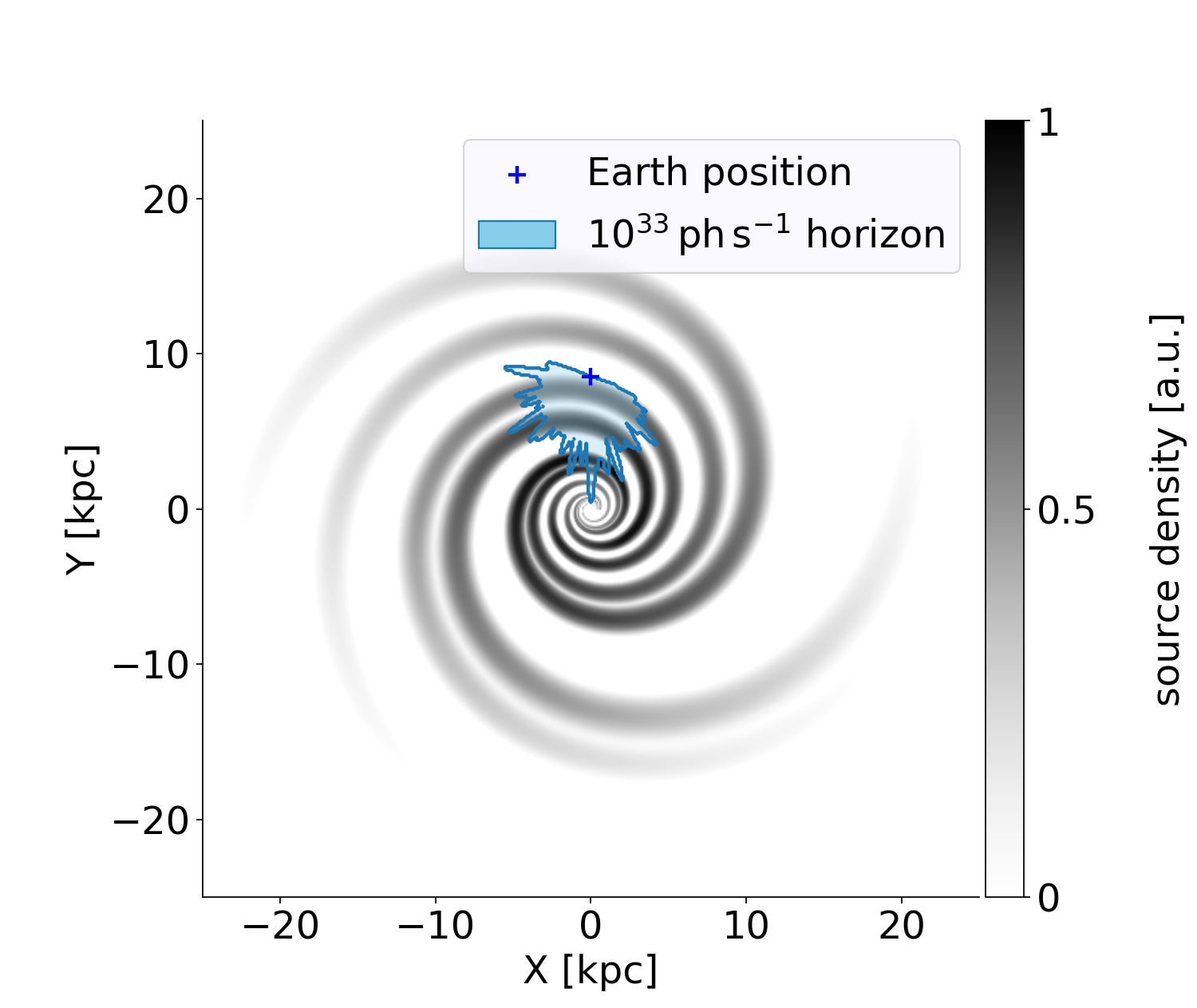
Figure 1: Distribution of VHE sources in the Milky Way following the four-arm spiral model by Steiman-Cameron et al. (2010) as described in Sec. 2 (grey contours). Additionally, the HGPS detection horizon for point-like sources with a luminosity of $10^{33}\,\mathrm{photons\,s^{-1}}$ is plotted on top (blue contours).

Besides the direction dependency, the sensitivity is also a function of the angular extent of a source since the number of background events increases with $\sigma_{source}$. To exceed the detection threshold of $5\sigma$ above background, the flux of an extended source needs to be greater than

$$F_{min}(\sigma_{source})=\cases{F}_{min,0}\sqrt{\frac{\sigma_{source}^{2}+\sigma_{PSF}^{2}}{\sigma_{PSF}^{2}}},&\leq 1^{\circ}\\ \infty,>1^{\circ}{}$$ (8)

(H.E.S.S. Collaboration et al. 2018c), where $F_{min,0}$ is the point-source sensitivity, $\sigma_{source}$ the source extent, and $\sigma_{PSF}$ the size of the H.E.S.S. point-spread function (PSF). In addition, the limited FOV of the instrument in combination with the applied background subtraction technique of deriving background measurements from within the FOV renders sources $\gtrsim 1^{\circ}$ not detectable. For our purpose we adopted Eq. 8 to account for the fact that we only selected for extended sources. The HGPS does not provide a criterion for the minimal detectable extent of a source. Therefore, we set the threshold to the cited average value of the PSF ($\sigma_{PSF}=0.08^{\circ}$), which yields a sensitivity for extended sources that is written as

$$F_{min}^{\mathrm{extended}}(\sigma_{source})=\cases{\infty},&\sigma_{source}\leq\sigma_{PSF}\\ F_{min,0}\sqrt{\frac{\sigma_{source}^{2}+\sigma_{PSF}^{2}}{\sigma_{PSF}^{2}}},\sigma_{PSF}<\sigma_{source}\leq 1^{\circ}\\ \infty,1^{\circ}<\sigma_{source}\,.{}$$ (9)

We define the correction function as the fraction of detectable sources, namely sources within the adopted sensitivity range of the HGPS, in the total amount of sources in the FoV of the HGPS. Since the sensitivity decreases for faint or extended sources, the correction function depends on source properties, that is luminosity and radius $C(L,R)$.
Under the assumption that average source properties are identical throughout the Milky Way, we expect sources of any given properties to follow the same spatial distribution function. To calculate the correction function, we first derive the subset of sources which lie within the FOV of the HGPS from the set of simulated sources $S_{FoV}\subset S_{sim}$. Assigning each source the same luminosity $L$ and source radius $R$ we can then calculate the corresponding fluxes, angular extents, and locations in the sky as they would be observed at Earth. Based on these observables and the sensitivity limit (Eq. 9) of the HGPS, the subset of detectable sources for the given luminosity and radius can be derived $S_{det}(L,R)\subset S_{FoV}$. With this, a two-dimensional correction function $C(L_{i},R_{i})$ is derived for the same grid of source luminosities and radii mentioned above via

$$C(L_{i},R_{i})=0.32\cdot\displaystyle\sum_{\mathbf{x}\in S_{det}(L_{i},R_{i})}\rho\left(\mathbf{x}\right)/\displaystyle\sum_{\mathbf{x}\in S_{FoV}}\rho\left(\mathbf{x}\right)\,,$$ (10)

where $\rho$ is the source density corresponding to the assumed model. The additional factor $0.32$ accounts for the fact that $68\,\%$ of the detected sources are disregarded owing to missing distance estimates. The correction function for the spatial distribution model mSp4 is shown in Fig. 2 together with the distribution of HGPS sources that fulfil our selection criterion.

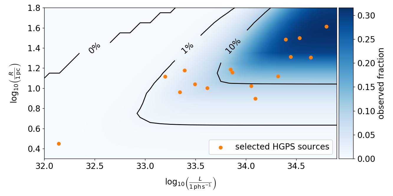
Figure 2: Estimated correction function for mSp4 showing the fraction of sources in the FOV of the HGPS that for a given luminosity and radius are detectable according to Eq. 9. The low values for small sources result from the rejection of point-like sources in the analysis. Additionally those sources of the HGPS that fulfil the selection criterion are shown.

Based on this estimation we show, for instance, that the distribution of the luminosity for $L<10^{33}\,\mathrm{ph\,s^{-1}}$ cannot be well constrained by the HGPS data. The estimation of the luminosity distribution in this regime is affected by statistical fluctuations of the data and special care has to be taken to explore the range of validity of the model.

2.2.3 Monte Carlo verification

We studied the capability of reconstructing properties of the parent population of the method presented in this work by the means of Monte Carlo simulations. For this purpose, we simulated source populations with a set of luminosity and radius functions for all spatial models discussed previously. For each simulated population, $N$ spatial coordinates $\mathbf{x}$ were randomly drawn following the distribution defined by Eq. 1, Eq. 2, or Eq. 2 + Eq. 3, according to the spatial model, with model specific parameters, together with $N$ random samples of $L$ and $R$ following Eq. 4 with the given parameters. For each combination of a luminosity and radius function and a source distribution, the subsample of detected sources was determined according to Eq. 9. As for the 50 extended sources detected with the HGPS the statistics of the simulated source population was adjusted to yield on average the same number of detected sources. To account for the fact that only a fraction of $32\,\%$ of the HGPS sources comes with a distance estimation, all but 16 of the detected simulated sources were randomly discarded. Each data set was then reconstructed using the machinery discussed before and the indices $\alpha_{L}$ and $\alpha_{R}$ of luminosity and radius functions were calculated. For each choice of spatial model and luminosity and radius function 600 populations were simulated and reconstructed. We performed these tests for all combinations of the indices $\alpha_{L}=-3,-2,-1$ and $\alpha_{R}=-2,-1,0$. For model mSp4 the mean of the reconstructed $\alpha$ values and their standard deviations are listed exemplarily in Table 3.

Table 3: Mean and standard deviation of the reconstructed $\alpha_{L}$ and $\alpha_{R}$ for the toy models using the spatial distribution of the four-arm spiral model of the ISM density (mSp4).

$\alpha_{R}$\$\alpha_{L}$	-3	-2	-1
-2	$\alpha_{L,reco}=-3.03\,\pm 0.38$	$\alpha_{L,reco}=-2.04\,\pm 0.28$	$\alpha_{L,reco}=-0.99\,\pm 0.30$
	$\alpha_{R,reco}=-2.04\,\pm 0.77$	$\alpha_{R,reco}=-1.92\,\pm 0.60$	$\alpha_{R,reco}=-1.96\,\pm 0.49$
-1	$\alpha_{L,reco}=-2.99\,\pm 0.36$	$\alpha_{L,reco}=-2.01\,\pm 0.29$	$\alpha_{L,reco}=-0.99\,\pm 0.38$
	$\alpha_{R,reco}=-1.05\,\pm 0.67$	$\alpha_{R,reco}=-0.96\,\pm 0.57$	$\alpha_{R,reco}=-0.94\,\pm 0.59$
0	$\alpha_{L,reco}=-3.01\,\pm 0.35$	$\alpha_{L,reco}=-2.00\,\pm 0.32$	$\alpha_{L,reco}=-1.03\,\pm 0.39$
	$\alpha_{R,reco}=0.01\,\pm 0.65$	$\alpha_{R,reco}=0.07\,\pm 0.63$	$\alpha_{R,reco}=0.08\,\pm 0.70$

For any combination, the mean of the reconstructed $\alpha$ agrees with the true value within $\Delta\alpha<0.1$. These results are remarkably consistent between spatial models. In particular, for all models and combinations of $\alpha_{L,\mathrm{true}}$ and $\alpha_{R,\mathrm{true}}$, the reconstructed $\alpha_{L}$ and $\alpha_{R}$ are always compatible with the true values of the simulations. An example is given in Fig. 3 showing for all spatial models the distribution of reconstructed $\alpha_{L}$ and $\alpha_{R}$ given true values of $\alpha_{L,\mathrm{true}}=-2$ and $\alpha_{R,\mathrm{true}}=-1$.

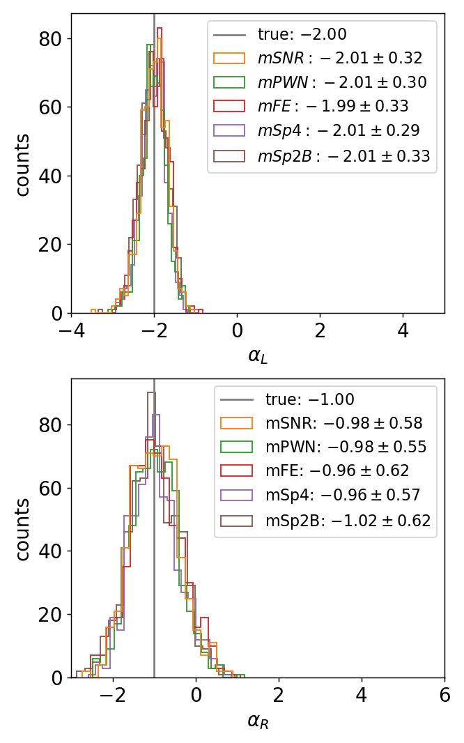
Figure 3: Distribution of reconstructed $\alpha_{L}$ (top) and $\alpha_{R}$ (bottom) for 600 toy models using different spatial models and true values of $\alpha_{L,\mathrm{true}}=-2$ and $\alpha_{R,\mathrm{true}}=-1$. True values are denoted by the vertical line.

The reconstructed values are always centred at their respective true values, with standard deviations around $0.3$ and $0.6$. We repeated this exercise for varying values to investigate the influence of the boundaries set on the luminosity and radius. No effect on the reconstructed $\alpha_{L}$ and $\alpha_{R}$ could be observed.
In Fig. 4, we show one-dimensional luminosity and radius distributions, which are derived from the 600 samples drawn from model mSp4 for $\alpha_{L,\mathrm{true}}=-2$ and $\alpha_{R,\mathrm{true}}=-1$.

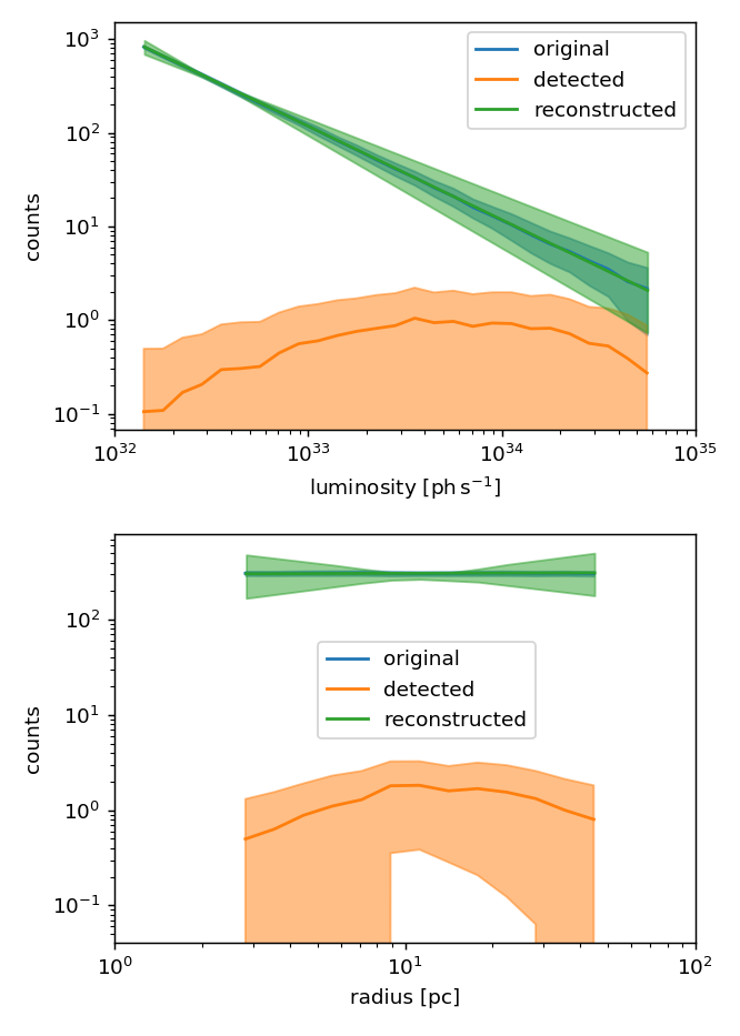
Figure 4: One-dimensional luminosity distribution (top) and radius distribution (bottom) for simulated populations. Original distributions are given in blue; distribution of detected sources in orange and the bias-corrected reconstruction of the original distribution are shown in green. Details are given in the text.

The blue line indicates the bin-wise mean of the luminosity and radius distribution for the whole population averaged over the 600 simulated samples, respectively. The blue shaded regions depicts the standard deviation accordingly. Likewise, the orange area shows the distribution for the selected samples, each comprised of 16 extended sources within the sensitivity range of the HGPS and with known $L$ and $R$. Besides the large spread of the latter distribution it is obvious that the distribution of detected sources on average does not resemble the global distribution. Therefore, it is inevitable for the reconstruction to properly account for the observation bias. The result of our reconstruction method is indicated in green. The solid line shows a power law with the mean reconstructed index. The power law is normed to the total number of sources of the simulated populations and perfectly matches the input distribution. The green shaded area represents the bin-wise quartile deviation.

2.2.4 Result

The derived power-law indices of $P(L,R)$ for the parent source population of the HGPS sample under the assumption of different underlying spatial source distributions are listed in Table 4. Again the results are fairly consistent among the spatial distributions with average values of $\left<\alpha_{L}\right>=-1.77$ and $\left<\alpha_{R}\right>=-1.26$. Owing to the small sample size used in this study the errors on these reconstructed values are expected to be comparable to those listed in Fig. 3 ($\Delta\alpha_{L}\sim 0.3$, $\Delta\alpha_{R}\sim 0.6$). Besides this statistical uncertainty, an additional cause of error is the choice of the boundaries of L and R. In general, deviations of the results due to this choice are found to be less than the stated errors, while the upper bound of the luminosity affects the reconstructed values most. However, this upper bound is well constrained since, according to the HGPS sensitivity, the chance of detecting a source with $L\geq 10^{34.8}\,\mathrm{ph\,s^{-1}}$ (disregarding the availability of a distance estimate) is close to one. In comparison, previous studies on the VHE source population not taking into account source sizes or the inhomogeneity of the sensitivity, have estimated the luminosity function to follow a power law with harder index (e.g. $-1>\alpha>-1.5$; Casanova & Dingus (2008)).

Table 4: Reconstructed power-law indices of the joint PDF $P(L,R)$ for different spatial distributions based on: a) SNRs (mSNR), b) PWNe (mPWN), c) free electrons (mFE), d) four-spiral arm model of the ISM density (mSp4), and e) two-spiral arm model of the ISM density with Galactic bar (mSp2B).

Model	$\alpha_{L}$	$\alpha_{R}$
mSNR	-1.70	-1.19
mPWN	-1.81	-1.13
mFE	-1.94	-1.21
mSp4	-1.64	-1.17
mSp2B	-1.78	-1.62

3 Comparison with observable quantities

In order to probe the validity of the derived models, for each model we compared the distribution of observable quantities from simulated source populations, namely Galactic longitude and latitude, fluxes, and angular extents, with those from observations. For each model a set $M$ of $3000$ synthetic source populations $S\in M$ were simulated. Because the distribution functions for source positions and source properties were fixed, we were able to estimate the total number of sources in the population based solely on the number of observed sources. Thus, it was not necessary to limit the analysed sample to extended sources, but we could increase the accuracy of our prediction by determining the expected number of detectable sources according to Eq. 8, including point-like sources, that match the 64 sources in the HGPS that pass this criterion. The numbers of sources per population for the individual models are listed in Table 6 and further discussed in Sec. 4.1. The distributions that are investigated in this section are solely derived from those detectable sources within the sensitivity range of the HGPS $S_{det}\subset S$ according to Eq. 8.

3.1 Flux and angular extent

The observed flux and angular extent of a source both depend on the distance of the source to the observer. In addition to this observational correlation, an intrinsic correlation between the luminosity and radius of sources can shape the observed distribution of fluxes and angular extents. Instrumental selection effects, such as the dependency of the sensitivity on the angular extent, can shape this distribution as well. To account for correlations, we compared the observed two-dimensional flux-extent distribution by means of its PDFs against the model prediction. We derived the PDFs from kernel density estimations for which the optimal bandwidth for a Gaussian kernel was derived individually in the range $[10^{-3},10]$ via the GridSearchCV method from the Python package scikit-learn. The distributions are very similar among the models, thus only the result for mSp4 is shown in comparison with the HGPS distribution in Fig. 5.

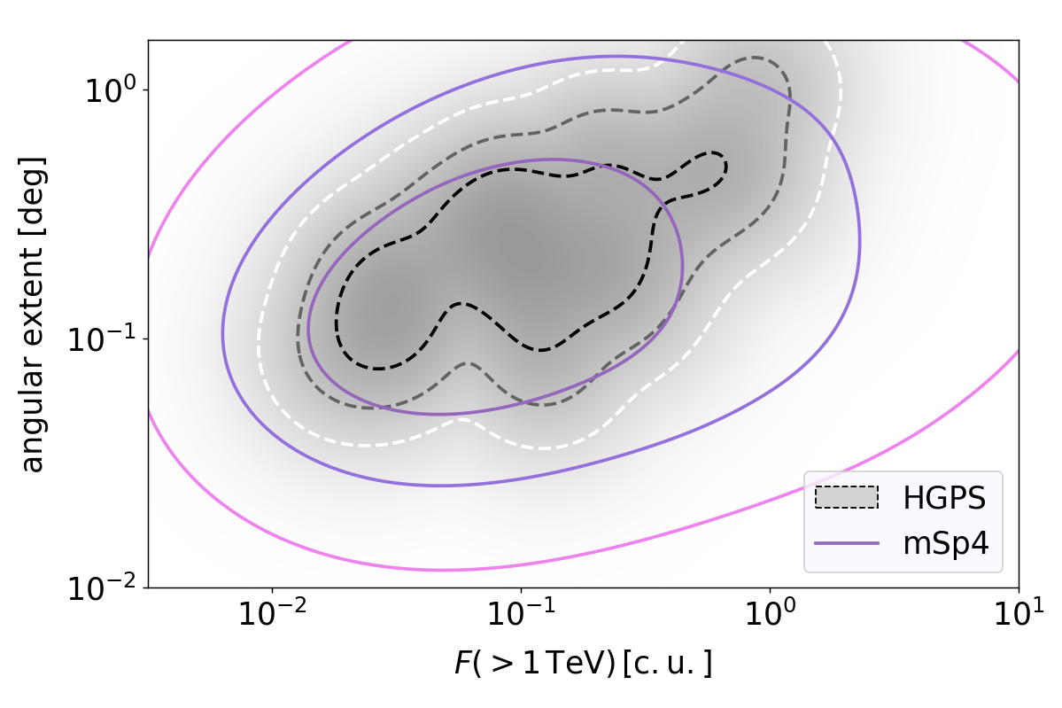
Figure 5: Kernel density estimation for the flux-extent distribution of the HGPS sample (grey) and mSp4 (orange). The contour lines indicate the $1\sigma$, $2\sigma,$ and $3\sigma$ containment fraction. Flux is given in ‘crab units’ (c.u.)

Contour lines indicate the $1\sigma$, $2\sigma$, and $3\sigma$ containment fraction of the derived PDFs for the observed distribution and the predicted distribution. For all distributions we observe an increase of the angular extent with flux, although this correlation appears less pronounced for the model distributions. Additionally, model distributions are noticeably wider than the observed distribution. This discrepancy is further reflected in the fraction of extended sources in the sample of detected sources. While for the HGPS we yield a fraction of $78\,\%$ (50 out of 64) of extended sources, for the models we observe on average a fraction between $23\,\%$ - $38\,\%$, the rest being point-like. This discrepancy might be an effect that is intrinsic to the HGPS. More point sources might be present in the data set but are “lost” in extended sources owing to source confusion (Ambrogi et al. 2016) or detected and later merged with an overlapping source. We did not account for these effects in our model. Alternatively, the model assumptions might not reflect reality and the number of point-like sources is overestimated: this might be an effect of the simplified definition of source extent, namely describing distinct and complex morphologies altogether by a single parameter. In addition, it is likely that the assumed independence of radius and luminosity and the power law for the source radius do not capture the true nature of this source property. Given the connection to the observation bias and especially the impact on the detectability of nearby sources, this relation is worth investigating in a follow-up study. Nevertheless, the flux-extent distribution of our models and observations are considered to be close enough to make reasonable predictions in the following.

3.2 Spatial distribution of sources

The source distributions in Galactic longitude for the probed models are depicted in Fig. 6.

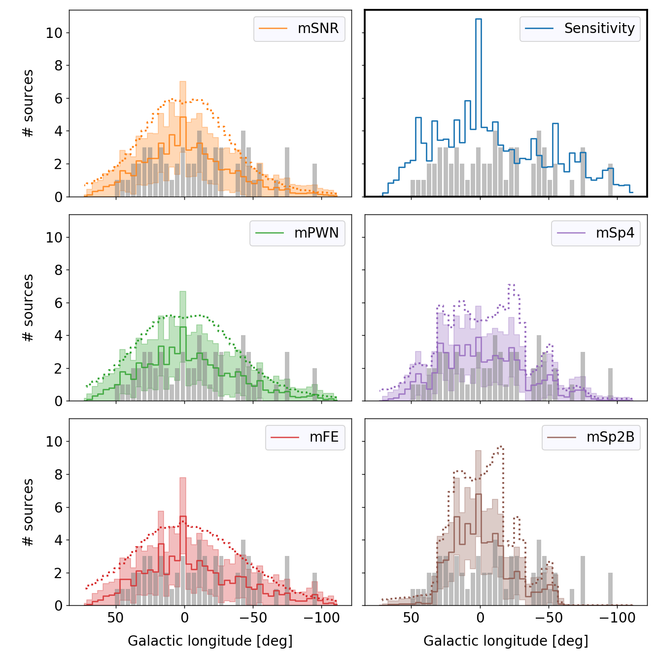
Figure 6: Comparison of the longitudinal source distribution between HGPS sources (grey bars) and predictions of different models (coloured lines). The dotted lines represent the modelled source densities within the HGPS region, arbitrarily scaled for the sake of visibility. In addition, the dynamic range of the HGPS sensitivity is shown on the top right panel. Details are given in the text.

The shaded region shows the standard deviation around the mean value of the different samples $S_{det}$ while the solid line represents the mean. For comparison, the observed distribution of the HGPS is given by the grey bars. Furthermore, the source density of the respective model within the FOV of the HGPS is shown by the dotted line, which is scaled for better visibility ($\int_{FoV}\rho(\mathbf{x})\,d\mathbf{x}=2N_{HGPS}$). On the top right panel of Fig. 6 the dynamic range of the sensitivity over Galactic longitude is shown, which is expressed by $F_{min}^{-3/2}$, where $F_{min}$ is the point-source sensitivity of the HGPS map at $b=0^{\circ}$ and the corresponding longitude bin. Here, for a given luminosity $F_{min}^{-3/2}$ is proportional to the sampled volume. For better visibility this distribution is scaled in the same way as the source densities.
The models are generally in good agreement with observations, although for mSp2B the longitude distribution appears to be somewhat too narrow as it falls off too steeply in the outskirts of the Galactic plane. The result for mSp2B suggests that if the ISM density distribution, which is used as proxy for the distribution of regions with high star formation rates, indeed follows the assumed shape, the VHE source population must comprise at least one source class that evolves outside those regions. In the central regions all models commonly tend to overpredict the actual source distribution. According to the models, this is the region of highest source density. Therefore, we can arguably expect that the detection of sources is also affected by source confusion and an increased background resulting from the existence of bright diffuse emission in the Galactic ridge region (H.E.S.S. Collaboration et al. 2006); both effects lead to a deficit of detected sources in that region. A future iteration of the model, taking both effects into account, will be required to unambiguously test whether this discrepancy in the central region can be attributed to an inaccurate spatial source distribution. Regarding the distribution of the source density we observe that, for model mSp4, peaks in this distribution align well with peaks in the observed source distribution. This might be suggestive that the Galactic population of VHE $\gamma$-ray sources indeed follows a similar spiral structure as derived from ISM measurements. However, with the inhomogeneity of the sensitivity, which yields similar distributions for detectable sources independently of the probed source distribution model, it is not feasible to make strong claims. Quantitatively we investigate the compatibility between model predictions and observations by means of the Kolmogorov-Smirnov test statistic $d_{n}$ as follows:

$$d_{n}=\sup_{x}\,\lvert F_{n}(x)-F_{0}(x)\rvert,$$ (11)

where $F(x)$ is the cumulative distribution over the variable $x$ (i.e. Galactic longitude). In this equation, $F_{0}(x)$ is derived from the mean distribution of a given model as shown by the solid line in Fig. 6. For each simulated population $d_{n}$ is calculated with the cumulative distribution $F_{n}(x)$ of detectable sources, yielding the probability distribution $P(d_{n})$. From the cumulative distribution of observed sources we derive $d_{HGPS}$ and calculate the p-value $P(d_{n}\geq d_{HGPS})$. The values listed in Table 5 confirm that only the longitude distribution of model mSp2B is incompatible with observations at a level of significance of $5\,\%$.

Table 5: Compatibility of the modelled longitude and latitude distribution with observations

	p-value
	longitude	latitude
mSNR	0.27	0.73
mPWN	0.52	0.36
mFe	0.77	0.08
mSp4	0.25	0.88
mSp2B	0.03	0.40

Source distributions in Galactic latitude are presented in Fig. 7 in the same way as for the longitudinal distributions.

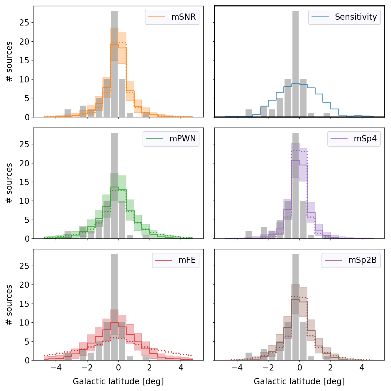
Figure 7: Comparison of the latitudinal source distribution as in Fig. 6

While for the latitude distribution all models are compatible with observations according to the statistical test, we can see some obvious deviation in this plot. The number of observed sources is falling rapidly outwards from the Galactic disc. The most prominent feature of the observed distribution is an asymmetry towards the southern sky that is not covered by any of the assumed models. Given that here we average over a broad source distribution over Galactic longitude, source confusion can be assumed to play a less pronounced role and the simulations correctly reflect the observation bias. Thus, this asymmetry appears to be a real feature of the spatial source distribution (cf. e.g. Skowron et al. (2019)), which is not accounted for in the models. Besides this, data show a stronger peak of the latitude distribution towards the Galactic equator compared to simulations. This is most notably the case for the model mFE, whose flatter distribution appears to be in tension with observation.

4 Global properties of the Galactic source population

While in the previous section it is shown that most models can describe observations reasonably well within the sensitivity range of the HGPS, in the following section these models are used to predict global properties of the Galactic VHE source population, namely the total number of sources in the Milky Way, their contribution to the observed $\gamma$-ray flux, and their cumulative luminosity.

4.1 Total number of sources

As described in Section 3, we can derive the average number of detectable sources $\left<N_{det}\right>$ according to Eq. 8 for any given total number of sources in a population $N_{tot}$: $\left<N_{det}(N_{tot})\right>$. With the probability of detecting 64 HGPS sources given by the Poissonian $P_{\left<N_{det}\right>}(64)$, the number of Galactic sources was derived from the maximum of the distribution $f\left(N_{tot}\right)=P_{\left<N_{det}\left(N_{tot}\right)\right>}(64)$ and cited errors from the corresponding $68\,\%$ containment area around this maximum. These numbers vary considerably among the probed models, ranging from 831 sources (mSp4) up to 7038 sources (mFE) (see Table 6).

Table 6: Population properties according to the probed models. The distribution of the total number of Galactic VHE $\gamma$-ray sources $N$ and their combined luminosity $L$ and flux $F$. The luminosities are characterised by the mean and standard deviation as this quantity is almost symmetrically distributed over the different realisations. In contrast, the median and quartile deviation are used as a more robust description of the total flux $F$, whose distribution is strongly affected by outliers that stem from (rare) nearby sources.

Model	$N$	$L$ [ph$\,\mathrm{s^{-1}}$]	$F$ [ph$\,\mathrm{cm^{-2}\,s^{-1}}$]
		Mean / Std	Median / QD
mSNR	$1063_{-126}^{+137}$	(1.73 / 0.16)$\,\cdot 10^{36}$	(4.89 / 1.41)$\,\cdot 10^{-10}$
mPWN	$2004_{-239}^{+259}$	(2.47 / 0.18)$\,\cdot 10^{36}$	(7.74 / 1.86)$\,\cdot 10^{-10}$
mFE	$7038_{-839}^{+912}$	(6.32 / 0.26)$\,\cdot 10^{36}$	(1.54 / 0.16)$\,\cdot 10^{-9}$
mSp4	$831_{-98}^{+107}$	(1.59 / 0.17)$\,\cdot 10^{36}$	(3.38 / 0.70)$\,\cdot 10^{-10}$
mSp2B	$1081_{-128}^{+140}$	(1.44 / 0.14)$\,\cdot 10^{36}$	(1.96 / 0.20)$\,\cdot 10^{-10}$

Although sources are treated generically as VHE $\gamma$-ray emitters in this model, that is no source type is explicitly assumed, a source count as high as seen for model mFE is challenging for the paradigm that SNRs and PWNe are the dominant source classes of VHE $\gamma$-ray emission. With a Galactic supernova rate of one per $40\,\mathrm{yr}$ (Tammann et al. 1994) a source count of 7000 implies a maximum age of emitters of $\sim 3\cdot 10^{5}\mathrm{yr}$. Interestingly, the models mSNR, mSp4, and mSp2B yield very similar results regarding the total number of sources. The similarity between model mSNR and mSp4 is also apparent in the cumulative source distribution over flux (log(N)-log(F)) as shown in Fig. 8, while mSp2B shows distinct differences.

Figure 8: Cumulative source distribution over flux (log(N)-log(F)). The HGPS source distribution is given by grey points with horizontal error bars depicting the bin width and vertical error bars showing the Poissonian error. Coloured lines represent the distribution of the whole Galactic source population averaged over the different realisations of the respective model. As the whole population also includes sources outside the FoV or too extended to be detectable, most models also overshoot the HGPS data in the range of completeness for point-like sources. Only mSp2B is in clear conflict with HGPS data.

In Fig. 8 the distribution of observed sources in the HGPS is given by grey points with Poissonian errors. The mean distribution for the whole Galactic population according to the different models is given by coloured lines. It appears that model mSp2B on average does not comply with the observed distribution, especially for $F>0.03\,\mathrm{c.u}$ (c.u.: integral flux of the Crab Nebula above $1\,\mathrm{TeV}$) yielding too few sources in this regime. In contrast, the other four models allow for sources of high flux (e.g. ¿ 0.1 c.u.) being undetected by the HGPS. The latter point is more clearly shown in Fig. 9.

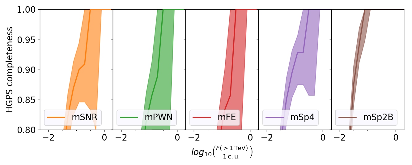
Figure 9: Fraction of detectable sources in the FOV of the HGPS cumulatively over source flux. The shaded regions represent the interquartile range; the lines depict the median.

In this figure the predicted completeness range of the HGPS is shown; more precisely, the figure shows the median fraction of detected sources within the FOV for sources exceeding a given flux level. This number decreases with decreasing flux levels as fainter sources are less likely to be detected. For most models a kink in the distribution is observed between $0.1\,\mathrm{c.u.}-1\,\mathrm{c.u.}$. That is caused by the limited sensitivity of imaging atmospheric Cherenkov telescopes (IACTs) to extended sources. For flat spatial source distributions the likelihood for close-by and, therefore, bright and extended sources to be found in the Galactic population increases. For model mSp4 we find that $2\pm 1$ and for model mPWN $3\pm 2$ sources exceeding the threshold of $1^{\circ}$ are expected to be found in the Galactic population. To probe this regime either different data analysis techniques or different observation techniques, for example with water Cherenkov telescopes that can make use of a large FOV, can be exploited. Indeed, two extended sources, Geminga (Abdo et al. 2007; Abeysekara et al. 2017) and 2HWC J0700+143 (Abeysekara et al. 2017), have been detected this way, which is in good agreement with both predictions.
Taking this one step further, we used these models to predict the number of sources that are detectable with the next generation of IACTs, CTA. Aiming for a point-source sensitivity of $2\,\mathrm{mCrab}$ in the longitude range $|l|<60^{\circ}$ and latitude range $|b|<2^{\circ}$ (Cherenkov Telescope Array Consortium et al. 2019), the predicted numbers of detectable sources lie in the range 295 (mSp4) - 457 (mFE). Since most of these sources are expected to appear point-like to CTA this number does not suffer considerably from a degradation of the sensitivity with source extent. Especially, this estimation is not affected by the inaccuracy of the description of source radii inherent to our models. The derived number is valid for the boundaries chosen for the luminosity. The implications for probing a larger dynamical range as it might be possible with CTA are discussed in Sec. 5. With the HGPS providing 53 sources in the region to be observed by the CTA Galactic plane scan, the CTA sample would increase the current source sample substantially by a factor between 5 - 9 according to these models.

4.2 Flux of unresolved sources

Although the HGPS is expected to comprise only $1\,\%-9\,\%$ of all sources in the Milky Way, these sources can already account for a significant fraction of the measurable flux (total flux given in Table 6). In Fig. 10 we give an illustrative example of one realisation of a synthetic VHE source population for model mSp4 in a face-on view of the Galaxy. For all of the 831 sources the luminosity and radius are encoded in the colour and radius of the circles representing them (radius not to scale), while sources that can be detected with the HGPS sensitivity are additionally denoted by an orange circle.

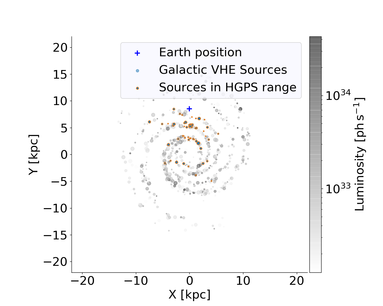
Figure 10: Example realisation of a synthetic population of VHE $\gamma$-ray sources for model mSp4. Source luminosities are given by the colour scale; source radii are proportional to circle radii. Detectable sources within the HGPS sensitivity are indicated with orange circles.

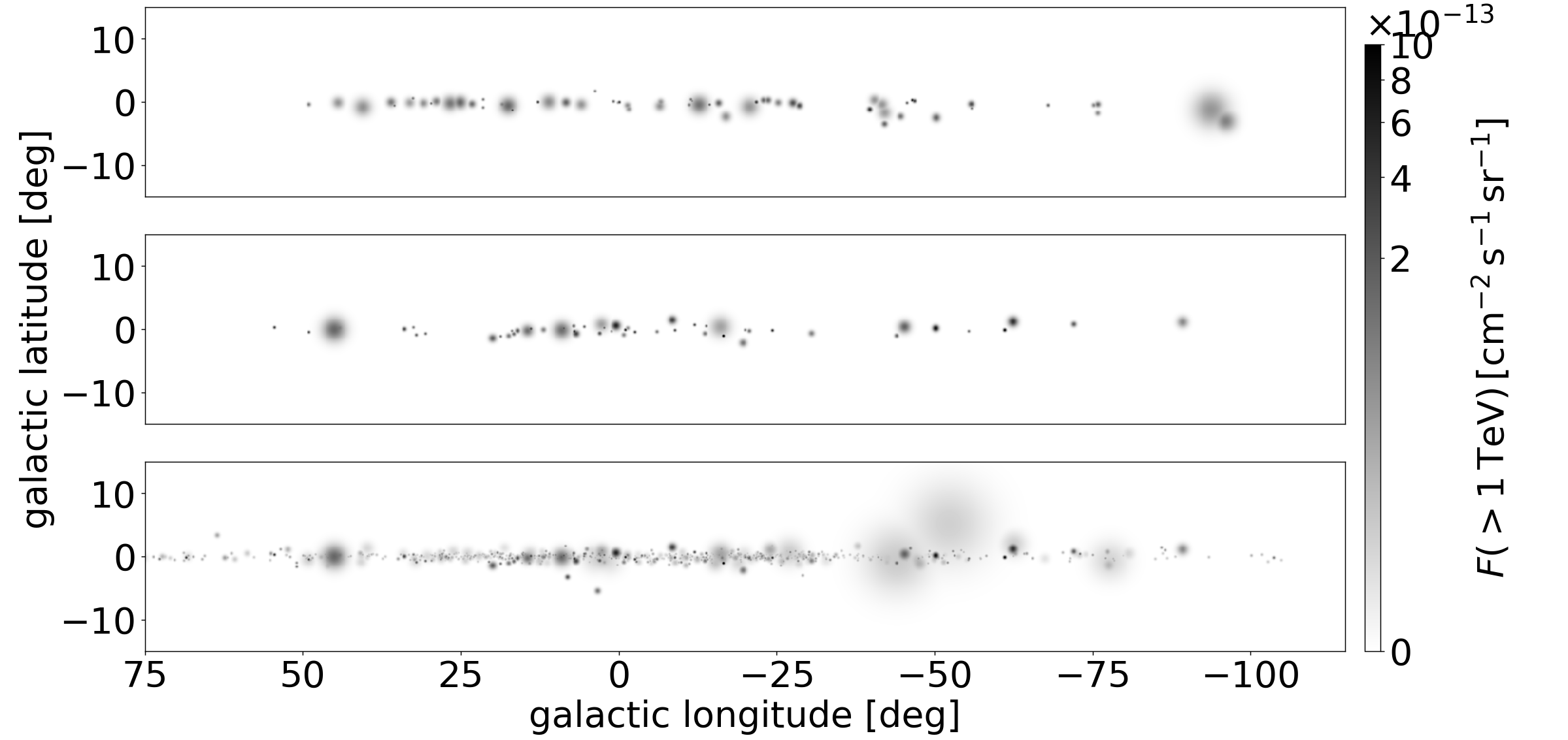
Figure 11: Sky maps of the VHE source population in the HGPS region. Top: From the HGPS catalogue. This map has been constructed by assuming a spherical source shape for better comparability with the simulations. Middle: Detectable sources from the synthetic population shown in Fig. 10, based on the mSp4 model. Bottom: All sources from this simulated realisation.

Corresponding sky maps of the fluxes for this realisation of the population are shown in Fig. 11. The middle panel of Fig. 11 shows the sample of detectable sources. In comparison with the HGPS sample shown in the top panel a similarity of the two samples is recognisable, although the HGPS clearly shows a larger fraction of extended sources. The discrepancy in the ratio of extended to point-like sources between observation and model prediction was already discussed in Sec. 3.1. The sky map of the same synthetic population when observed with infinite sensitivity is shown in the bottom panel of Fig 11. There, a band of faint sources along the Galactic plane, which can contribute to the unresolved, large-scale VHE $\gamma$-ray flux, is clearly seen. Focussing only on the region scanned by the HGPS, the flux of all sources detected by the HGPS exceeds the prediction of model mSp2B by $\sim 24\,\%$ as already indicated by the log(N)-log(F) distribution (see Fig. 8). The other four models predict that unresolved sources make up about $13\,\%-32\,\%$ of the total flux stemming from the source population within this region. The H.E.S.S. measurement of large-scale diffuse emission in the HGPS from regions that do not contain any significant $\gamma$-ray emission quotes a similar number of $\sim 28\,\%$ of the total measured VHE emission in large-scale diffuse emission (H.E.S.S. Collaboration et al. 2014). However, these numbers are not directly comparable since the sky regions they are derived from are not identical. While the model allows us to remove detectable sources easily, complex exclusion regions were applied for the H.E.S.S. measurement to exclude contribution from sources, most of which accumulate at small Galactic latitude values. Still, these numbers are suggestive that unresolved sources might very well be the dominant component of the measured diffuse emission.
Additionally, the two prominent extended sources that are seen at $\sim-50^{\circ}$ longitude on the sky map at the bottom of Fig. 11, but not in the sky map in the centre, demonstrate the effect of the maximum extent detectable by H.E.S.S., which has been discussed with respect to the catalogue completeness (see Sec. 4.1).

4.3 Luminosity of the Galactic source population

Using the mean photon energy of $3.52\,\mathrm{erg\,ph^{-1}}$ from Sec. 2.2, the total luminosity of the Galactic VHE source population is estimated to lie in the range $(5.07\cdot 10^{36}-2.22\cdot 10^{37})\,\mathrm{erg\,s^{-1}}$. Assuming that $\gamma$-ray sources are the dominant contribution to the overall VHE $\gamma$-ray luminosity of the Milky Way and that the diffuse emission originating from propagating cosmic rays adds only a small contribution, these values can be compared with the total luminosity at megaelectronvolt and gigaelectronvolt energies ($\sim 3\cdot 10^{38}\,\mathrm{erg\,s^{-1}}$ and $\sim 8\cdot 10^{38}\,\mathrm{erg\,s^{-1}}$, respectively; Strong et al. (2010)). The $\gamma$-ray luminosity of the Milky Way at VHE turns out to be one to two orders of magnitude lower than in those two lower energy bands. This demonstrates that the presented models are compatible within the available energy budget constraints and indicates a drop in luminosity between the HE and VHE ranges.

5 Conclusions

We present models of the VHE $\gamma$-ray source population of the Milky Way, based on different assumptions of the spatial source distributions. Power-law indices of luminosity and radius functions of the population are derived from a subsample of the HGPS source catalogue (namely, extended sources with known distances) and its sensitivity. We pay special attention to correction of the observation bias. The validation of this bias correction is done with simulated toy models and demonstrates very good reconstruction capabilities. Furthermore, the simulations demonstrate that relying on the detected set of sources with no bias correction gives more or less arbitrary results. In this context it has to be noted that the limitation to the range of completeness does not completely avoid this problem because the completeness relates to point-like sources and does not apply to sources of larger extension.
A comparison of the source models with HGPS observations demonstrates a reasonable agreement. Despite a lack of asymmetry in the latitude distribution seen in all models as compared to the observed distribution (see Fig. 7), simulations approximately reproduce the spatial HGPS source distribution as well as the distribution of source fluxes and extents. Only the model mSp2B is disfavoured owing to its distinctively different longitude distribution in the HGPS sensitivity range and the clear under-prediction of the total flux from VHE $\gamma$-ray sources. All models under-predict the fraction of extended sources in the detectable sample, which can be attributed to either effects in the construction of the HGPS catalog (e.g. source confusion) or shortcomings of the model (e.g. invalidness of underlying assumptions) or a combination of both.
Despite the rather limited statistics in the sample of HGPS sources, our data-driven approach, which minimises the degrees of freedom, allows for relatively good predictions to be made. The derived models can be used to study possibilities and limitations of VHE observations. Examples are expectations for future instruments, an assessment of the amount of yet unresolved sources in a large-scale diffuse emission measurement depending on the sensitivity threshold, and the study of observational challenges like source confusion. We derived the total number of VHE sources in the Milky Way and the total luminosity and flux of the Milky Way in VHE $\gamma$-rays. Disregarding the one disfavoured model, of the four remaining models, mPWN, mSNR, and mSp4 do not deviate substantially from one another. While model mFE also yields similar results regarding the distribution of source properties, the predicted number of sources within the Milky Way exceeds the predictions of the other models by a factor $>3$. Thus, the predicted range of VHE sources in our Galaxy is 800 to 7000. The scatter in the total luminosity and the total flux lies with a factor $\sim 4$ in the range of $(1.6-6.3)\cdot 10^{36}$ ph s^-1 and $(3-15)\cdot 10^{-10}$ ph cm^-2 s^-1, respectively. A significant fraction, $(13-32)\%$, of the $\gamma$-ray emission of sources within the HGPS region is attributed to yet unresolved sources and contributes to the measured diffuse emission. With a foreseen sensitivity of $2\,\mathrm{mCrab}$ in the central Galactic plane, CTA should be able to increase the known Galactic VHE $\gamma$-ray source sample by a factor between 5 - 9.
It should be noted that the derived properties depend not only on the chosen spatial distribution model but also on the luminosity range covered by the model. Especially, the low-luminosity limit can have a significant impact on the expected number of sources and the energy budget. The choice of this limit was made to encompass the HGPS data, and it is possible that weaker sources (or a subdominant class of less luminous sources) can be on the verge of detection and not being identified with the present, inhomogeneous sensitivity. Expanding the dynamical range towards lower luminosities in the models increases the fraction of sources that lie outside the sensitivity limit and thus increases the expected number of VHE sources in the Galaxy and simultaneously increases (although to a lesser degree) predictions for fluxes and luminosities. Another factor that affects the estimation of the size of the population is source confusion. Given the predicted number of sources in the Galaxy, confusion of sources in the FOV and their ascribed fluxes seems to be inevitable. If source confusion already underlies the HGPS detected data set, the true size of the VHE source population can be expected to be even larger and luminosity and radius functions are subject to an additional bias.
Consequently, improvements of these models planned for the future include the correct treatment of source confusion in the comparison between simulations and data. Additionally, inclusion and proper treatment of sources with incomplete information (point-like sources/no known distance estimation) can increase the statistics of the sample. The incorporation of spectral information will allow for comparisons with neighbouring energy bands, making use of the wealth of information at Fermi-LAT energies and the complementarity of wide FOV HAWC observations.
In order to study the physics of VHE $\gamma$-ray sources, differentiation is required between the various source classes, such as SNRs and PWNe as the likely dominating contributors, and smaller contributions from other classes. This goes in conjunction with a widening of the parameter space that is needed to include physical source properties rather than the phenomenological observables used in this work. Although weakly constrained with the currently available data, this inclusion of physical source modelling for the characterisation of the population properties of VHE source classes is the logical next step after the in-depth studies of single objects and the description of the detected samples of sources so far performed with HGPS data (see e.g. Cristofari et al. (2013, 2017)). The presented models can serve as a basis for such studies. With future surveys of more sensitive instruments such as CTA the amount of available data will increase, allowing for more accurate characterisations of the SNR and PWN populations.