Characterising Bias in Compressed Models

Abstract

The popularity and widespread use of pruning and quantization is driven by the severe resource constraints of deploying deep neural networks to environments with strict latency, memory and energy requirements. These techniques achieve high levels of compression with negligible impact on top-line metrics (top-1 and top-5 accuracy). However, overall accuracy hides disproportionately high errors on a small subset of examples; we call this subset Compression Identified Exemplars (CIE). We further establish that for CIE examples, compression amplifies existing algorithmic bias. Pruning disproportionately impacts performance on underrepresented features, which often coincides with considerations of fairness. Given that CIE is a relatively small subset but a great contributor of error in the model, we propose its use as a human-in-the-loop auditing tool to surface a tractable subset of the dataset for further inspection or annotation by a domain expert. We provide qualitative and quantitative support that CIE surfaces the most challenging examples in the data distribution for human-in-the-loop auditing.

1 Introduction

Pruning and quantization are widely applied techniques for compressing deep neural networks, often driven by the resource constraints of deploying models to mobile phones or embedded devices (Esteva et al., 2017; Lane & Warden, 2018). To-date, discussion around the relative merits of different compression methods has centered on the trade-off between level of compression and top-line metrics such as top-1 and top-5 accuracy (Blalock et al., 2020). Along this dimension, compression techniques are remarkably successful. It is possible to prune the majority of weights (Gale et al., 2019; Evci et al., 2019) or heavily quantize the bit representation (Jacob et al., 2017) with negligible decreases to test-set accuracy.

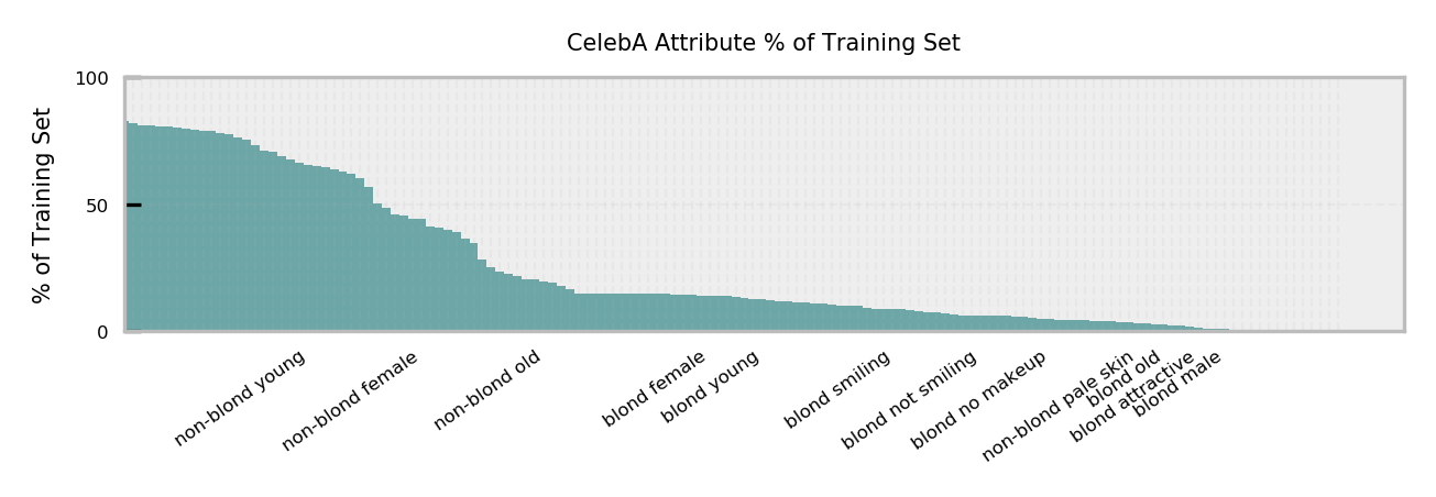
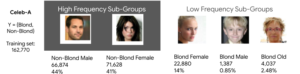
Figure 1: Most natural image datasets exhibit a long-tail distribution with an unequal frequency of attributes in the training data. Below each attribute sub-group in CelebA, we report the share of training set and total frequency count.

However, recent work by Hooker et al. (2019b) has found that the minimal changes to top-line metrics obscure critical differences in generalization between pruned and non-pruned networks. The authors establish that pruning disproportionately impacts predictive performance on a small subset of the dataset. We build upon this work and focus on the implications of these findings for a dataset with sensitive protected attributes such as gender and age. Our work addresses the question: Does compression amplify existing algorithmic bias?

Understanding the relationship between compression and algorithmic bias is particularly urgent given the widespread use of compressed deep neural networks in resource constrained but sensitive domains such as hiring (Dastin, 2018; Harwell, 2019), health care diagnostics (Xie et al., 2019; Gruetzemacher et al., 2018; Badgeley et al., 2019; Oakden-Rayner et al., 2019), self-driving cars (NHTSA, 2017) and facial recognition software (Buolamwini & Gebru, 2018b). For these tasks, the trade-offs incurred by compression may be intolerable given the impact on human welfare.

We establish consistent results across widely used quantization and pruning techniques and find that compression amplifies algorithmic bias. The minimal changes to overall accuracy hide disproportionately high errors on a small subset of examples. We call this subset Compression Identified Exemplars (CIE). Given two model populations, one compressed and one non-compressed, an example is a CIE if the labels predicted by the compressed population diverges from the labels produced by the non-compressed population.

Reasoning about model behavior is often easier when presented with a subset of data points that is atypical or hard for the model to classify. Our work proposes CIE as a method to surface a tractable subset of the dataset for auditing. One of the biggest bottlenecks for human auditing is the large scale size of modern datasets and the cost of annotating each feature (Veale & Binns, 2017). For many real-world datasets, labels for protected attributes are not available. In this paper, we show that CIE is able to automatically surface more challenging examples and over-indexes on the protected attributes which are disproportionately impacted by compression. CIE is a powerful unsupervised protocol for auditing. Given that the methodology is agnostic to the presence of attribute labels, CIE allows us to audit multiple attributes all at once. This makes CIE a potentially valuable human-in-the-loop auditing tool for domain experts when labels for underlying attributes are limited.

In Section. 2, we firstly establish the degree to which model compression amplifies forms of algorithmic bias using traditional error metrics. Section. 3 introduces different measures of CIE and motivates the use of CIE as an auditing tool for surfacing these biases when labels are not available for the underlying protected attributes. In Section. 3.2 we discuss a human-in-the-loop protocol to audit compression induced error.

2 Characterising Compression Induced Bias in Data with Sensitive Attributes

Recent studies have exposed the prevalence of undesirable biases in machine learning datasets. For example, Buolamwini & Gebru (2018a) discuss the disparate treatment of darker skin tones due to under-representation within facial analysis datasets, object detection datasets tend to under-represent images from lower income and non-Western regions (Shankar et al., 2017; DeVries et al., 2019), activity recognition datasets exhibit stereotype-aligned gender biases (Zhao et al., 2017), and word co-occurrences within text datasets frequently reflect social biases relating to gender, race and disability (Garg et al., 2017; Hutchinson et al., 2020).

In the absence of fairness-informed interventions, trained models invariably reflect the undesirable biases of the data they are trained on. This can result in higher overall error rates on demographic groups underrepresented across the entire dataset and/or false positive rates and false negative rates that skew in alignment with the over- or under-representation of demographic groups within a target label.

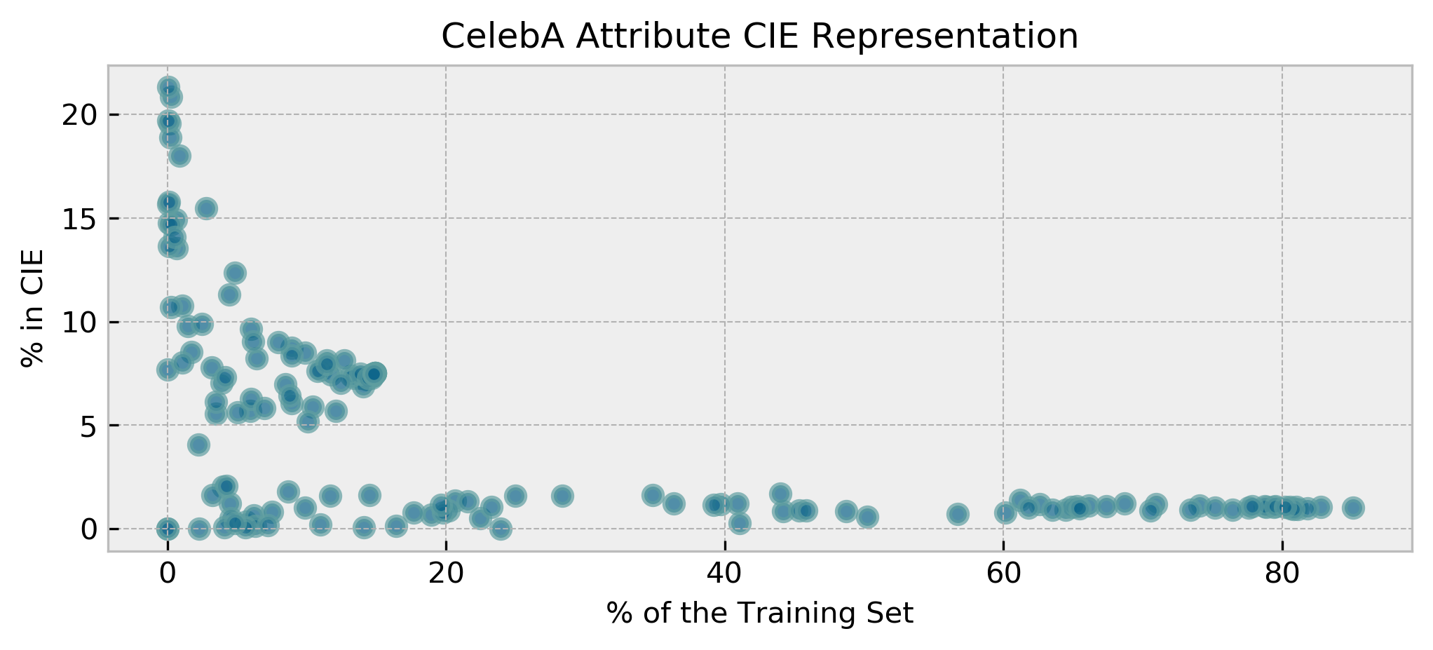
Figure 2: Plot of the fraction of the training set of each attribute in CelebA against the relative representation of each attribute in CIE_p. CIE_p over-index on underrepresented attributes in the dataset. In this plot we threshold Taxicab CIE generated from a pruned model at $80\%$.

In this section, we firstly establish the degree to which model compression amplifies forms of algorithmic bias using traditional error metrics. Our analysis leverages CelebA (Liu et al., 2015), a dataset of celebrity faces annotated with 40 binary face attributes and trains a classifier to predict a binary label indicating if the Blonde hair attribute is present. The CelebA dataset is well-suited for our analysis due to the significant correlations between protected demographic groups and the target label (defined by Blonde), as well as the overall under-representation of some demographic groups across the training dataset. As seen in Figure 1, CelebA is representative of many natural image datasets where attributes follow a long-tail distribution (Zhu et al., 2014; Feldman, 2019).

2.1 Methodology

Our goal is to understand the implications of compression on model bias and fairness considerations. Thus, we focus attention on two protected unitary attributes Male and Young and one intersectional attribute from the combination of these unitary attributes (i.e Young Male). To characterize the impact of compression on age and gender sub-groups we compare sub-group error rate, false positive rate (FPR) and false negative rate (FNR) between a baseline (i.e. non-compressed) and models pruned and quantized to different levels of compression (i.e. compressed).

We evaluate three different compression approaches: magnitude pruning (Zhu & Gupta, 2017), fixed point 8-bit quantization (Jacob et al., 2017) and hybrid 8-bit quantization with dynamic range (Williamson, 1991). In contrast to the pruning which is applied progressively over the course of training, all of the quantization methods we evaluate are implemented post-training. For all experiments, we train a ResNet-18 (He et al., 2015) on CelebA for $10,000$ steps with a batch size of $256$.

Pruning Protocol

For pruning, we vary the end sparsity for $t\in\{0.3,0.5,0.7,0.9,0.95,0.99\}$. For example, $t=0.9$ indicates that $90\%$ of model weights are removed over the course of training, leaving a maximum of $10\%$ non-zero weights at inference time. For the pruning variants, we prune every $500$ steps between $1000$ and $9000$ steps. These hyperparameter choices were based upon a limited grid search which suggested that these particular settings minimized degradation to test-set accuracy across all pruning levels. At the end of training, the final pruned mask is fixed and during inference only the remaining weights contribute to the model prediction. To move beyond anecdotal observations, we train $30$ models for every level of compression considered. Our goal is to have a high level of certainty that differences in predictive performance between compressed and non-compressed models is statistically significant and not due to inherent noise in the stochastic training process of deep neural networks.

CelebA
Fraction Pruned	Top 1	# Modal CIEs
0	94.73	-
0.3	94.75	555
0.5	94.81	638
0.7	94.44	990
0.9	94.07	3229
0.95	93.39	5057
0.99	90.98	8754
Quantization	Top 1	# Modal CIEs
hybrid int8	94.65	404
fixed-point int8	94.65	414

Table 1: CelebA top-1 accuracy at all levels of pruning, averaged over runs. The task we consider for CelebA is a binary classification method. We consider exemplar level divergence and classify Compression Identified Exemplars as the examples where the modal label differs between a population of $30$ compressed and non-compressed models. Note that the CelebA task is a binary classification task to predict whether the celebrity is blond or non-blond. Thus, there are only two classes. ***Note that the number of Taxicab CIEs are just the fraction of the threshold -ie if we threshold at 90% then the number of CIEs will be 10% of the dataset.

Quantization Protocol

We use two types of post-training quantization. The first type uses a hybrid ”dynamic range“ approach with 8-bit weights (Alvarez et al., 2016). The second type uses fixed-point only 8-bit weights (Vanhoucke et al., 2011; Jacob et al., 2018), with the first 100 training examples of each dataset as representative examples. Each of these quantization methods has open source code available. We use the MLIR implementation via TensorFlow Lite (Jacob et al., 2018; Lattner et al., 2020).

2.2 Results

Our baseline non-compressed model obtains $94.73\%$ mean top-1 test-set accuracy (top-5 accuracy is not salient here as it is a binary classification task). Table 5 (top row) shows baseline error metrics across unitary and intersectional subgroups. There is a very narrow range of difference in overall test-set accuracy between this baseline and the different compression levels we consider. For example, after pruning $90\%$ and $95\%$ of network weights the top-1 test-set accuracy is $94.07\%$ and $93.39\%$ respectively. Table 2 provides details of performance at all compression levels for both pruning and quantization.

CelebA Top-1 Accuracy
	Modal CIEs		Taxicab CIEs
Fraction Pruned	CIEs	All	90th	95th	99th
30.0	49.82	94.75	63.58	58.49	55.35
50.0	50.55	94.81	63.06	58.88	54.44
70.0	52.61	94.44	64.08	61.36	55.29
90.0	50.41	94.07	62.35	56.60	50.10
95.0	45.57	93.39	60.53	51.99	43.43
99.0	39.84	90.98	49.93	39.75	29.21
Quantization
hybrid int8	48.90	94.65	61.69	54.89	45.65
fixed-point int8	48.13	94.65	61.68	54.41	45.15

Table 2: A comparison of model performance on Compression Identified Exemplars (CIE) relative to performance on the test-set and a sample excluding CIEs (non-CIEs). Evaluation on CIE images alone yields substantially lower top-1 accuracy. Note that CelebA top-5 is not included as it is a binary classification problem.

How does compression amplify existing model bias? We find that compression consistently amplifies the disparate treatment of underrepresented protected subgroups for all levels of compression that we consider. While aggregate performance metrics are only minimally affected by compression – albeit with FNR being amplified to a greater extent that FPR – we clearly see the newly introduced errors are unevenly distributed across sub-groups. For example,the middle row of Table 3 shows that at 95% pruning FPR for Male has a normalized increase of $49.54\%$ relative to baseline. In contrast, there is far more minimal impact on not Male with a normalized relative increase of only $6.32\%$. This is less than the overall change in FPR ($12.72\%$). We note that this appears closely tied to the overall representation in the dataset, with Blond not Male constituting $14\%$ of the training set versus Blond Male with only $0.85\%$. Compression cannibalizes performance on low-frequency attributes in order to preserve overall performance. In Table 4 we show that higher levels of compression only further compound this disparate treatment.

			Unitary				Intersectional
Model	Metric	Aggregate	M	F	Y	O	MY	MO	FY	FO
Baseline	Error	5.30%	2.37%	7.15%	5.17%	5.73%	2.28%	2.50%	5.17%	5.73%
(0% pruning)	FPR	2.73%	0.93%	4.12%	2.59%	3.18%	0.81%	1.12%	2.59%	3.18%
	FNR	22.03%	62.65%	19.09%	21.35%	24.47%	60.45%	66.87%	21.35%	24.47%
Normalized Difference Between 1) Compressed and 2) Non-Compressed Baseline
Compressed	Error	24.63%	24.49%	24.67%	20.64%	35.84%	7.96%	49.12%	20.64%	35.84%
(95% pruning)	FPR	12.72%	49.54%	6.32%	3.35%	36.02%	5.37%	101.88%	3.35%	36.02%
	FNR	34.22%	8.41%	40.30%	33.83%	35.39%	9.21%	6.98%	33.83%	35.39%

Table 3: Performance metrics disaggregated across Male (M), not Male (F), Young (Y), and not Young (O) sub-groups. For all error rates reported, we average performance over $10$ models. Top Row: Baseline error rates, Bottom Row: Relative change in error rate between baseline models and models pruned to 95% sparsity,

3 Auditing Compressed Models in Limited Annotation Regimes

In the previous section, we established that compressed models amplify existing bias using traditional error metrics. However, the auditing process we used and conclusions we have drawn required the presence of labels for protected attributes. The availability of labels is often highly infeasible in real-world settings (Veale & Binns, 2017) because of the cost of data acquisition and privacy concerns associated with annotating protected attributes. In this section, we propose Compression Identified Exemplars (CIEs) as an auditing tool to surface a tractable subset of the data for further inspection or annotation by a domain expert. Identifying a small sample of examples that merit further human-in-the-loop annotation is often critical given the large scale size of modern datasets. CIEs are where the predictive behavior diverges between a population of independently trained compressed and non-compressed models.

Blonde
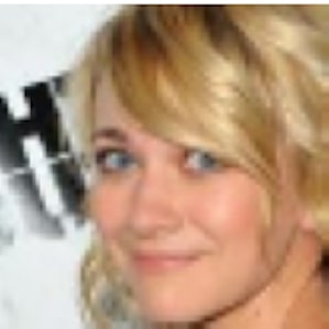
Non-CIE	Non-CIE	Non-CIE		CIE	CIE	CIE
Non-Blonde
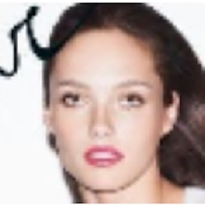
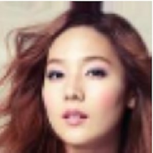
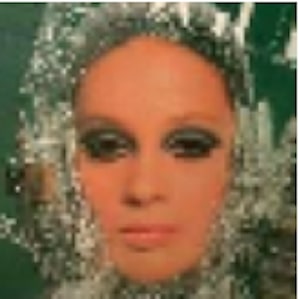
Non-CIE	Non-CIE	Non-CIE		CIE	CIE	CIE

Figure 3: Compression Identified Exemplars (CIEs) are images where there is a high level of disagreement between the predictions of pruned and non-pruned models. Visualized are a sample of CelebA CIEs alongside a non-CIE image from the same class. Above each image pair is the true label. We train a ResNet-18 on CelebA to predict a binary task of whether the hair color is blond or non-blond.

Metric	Aggregate	Unitary sub-groups		Intersectional sub-groups
Error
FPR
FNR

Table 4: For each unitary and intersectional sub-group, we plot the normalized difference of the compressed model, at each level of sparsity (x-axis), relative to the non-compressed model. Note that we threshold the y-axis limit at $100$ for the purposes of standard comparison. Top row: Aggregate error, Middle row: False Positive Rate (FPR), Bottom row: False Negative Rate (FNR)

3.1 Divergence Measures

In additional to the measure of divergence proposed by proposed by Hooker et al. (2019b) which we term Modal CIE, we consider an additional measure of divergence Taxicab CIE. We briefly introduce both below. We provide a proof in the appendix of the equivalence of CIE-selection algorithms based on the Jaccard and Taxicab distances.

Modal CIE

Hooker et al. (2019b) For set $Y^{*}_{x,t}$ we find the modal label, i.e. the class predicted most frequently by the $t$-compressed model population for exemplar $x$, which we denote $y^{M}_{x,t}$. Exemplar $x$ is classified as a Modal CIE_t if and only if the modal label is different between the set of $t$-compressed models and the non-compressed models:

$$\textit{CIE}{}_{x,t}=\begin{cases}1&\text{if $y^{M}_{x,0}\neq y^{M}_{x,t}$}\\ 0&\text{otherwise}\end{cases}$$

Taxicab CIE

We compute Taxicab distance as the absolute difference between the distribution of labels $y^{M}_{0}$ from the baseline models and the set $y^{M}_{t}$ from the compressed models. Given an example $x$, define $B_{x}=\{b_{x,i}\}$ to be the distribution of labels from a set of baseline models where $b_{x,i}$ is the number of baseline models that label example $x$ with class $i$. Similarly define $V_{x}=\{v_{x,i}\}$ to be the distribution of labels from a set of variant models where $v_{x,i}$ is the number of variant models that label example $x$ with class $i$.

Let $d_{T}$ be the Taxicab distance between two label distributions,

$$d_{T}(B_{x},V_{x})=\sum_{i}|b_{x,i}-v_{x,i}|.$$

Difference between measures proposed While Modal CIE identifies all examples with a changing median label as CIE, Taxicab CIE scores the entire dataset allowing for a ranking that can be thresholded by a domain user. Both methods of auditing require no labels for the underlying attributes. That said, note that this turns into a limitation in an overfit $0\%$ training error regime as without any predictive difference it would not be possible to compute CIE using either measure in the training set.

3.2 Does ranking by CIE identify more challenging examples?

Surfacing Challenging Examples CIE

Here, we explore whether CIE divergence measures are able to effectively discriminate between easy and challenging examples. In Table. 2, we find that at all levels of compression considered, both CIE metrics surface a subset of data points that are far more challenging for both compressed and non-compressed models to classify. For example, while the baseline non-compressed top-1 test set performance on the entire test set is $94.76\%$, it degrades sharply to $49.82\%$ and $55.35\%$ when restricted to Modal CIE (for CIE computed at $t=0.9$) and Taxicab CIE (at percentile $99\%$) respectively. It is hard to compare explicitly the relative difficulty of Modal CIE and Taxicab CIE because the sample sizes are not ensured to be equal. In the appendix, we include the absolute test-set accuracy on a range of Taxicab CIE percentiles and different levels of pruning (Table.). While while examples which are Modal CIE are more challenging than those identified by Taxicab CIE, for most points of comparison, the results support Taxicab CIE as an effective ranking technique across the entire dataset and evidences a monotonic degradation in test-set accuracy as percentile is increased.

Top-1 Accuracy on CIE, All Test-Set, Non-CIE

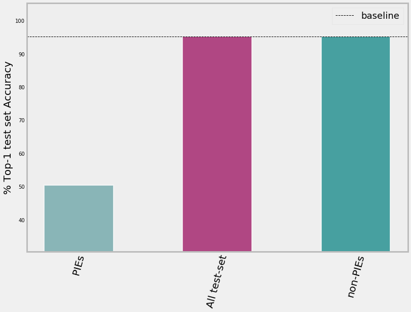
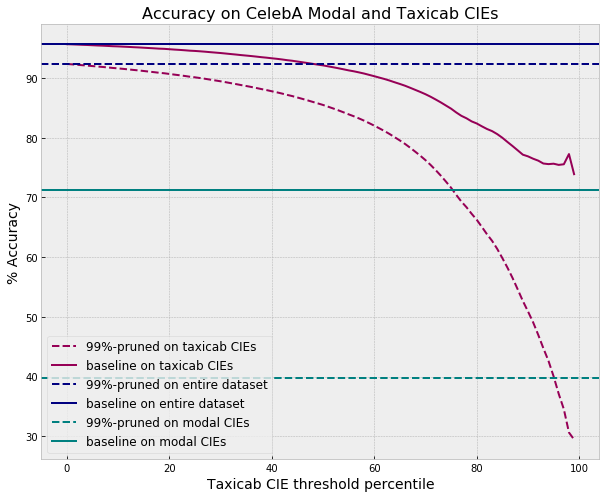
Figure 4: Right: A comparison of model performance on $1$) a sample of Modal CIEs against the, $2$) the entire test-set and $3$) a sample excluding CIEs. Evaluation on CIE images alone yields substantially lower top-1 accuracy, Left: Comparison of non-compressed test-set accuracy (solid lines) against compressed $t=99$ pruned test-set accuracy (dashed lines) on 1) the entire test-set, with 2) Modal CIE identified at $99\%$ pruning and 3) Taxicab CIE thresholded at different percentiles (x-axis). Any ties for Taxicab CIE are broken at random. Images with high Taxicab CIE scores and or classified as Modal CIE are far more challenging for both the non-compressed and compressed model to classify.

Amplified sensitivity of compressed models to CIE

In Fig. 4, we plot the test-set accuracy of examples bucketed by Modal CIE and Taxicab CIE. Overall accuracy drops by less than 3% between the baseline and pruned models when evaluated on the overall test-set. However, the difference in performance is much larger when we restrict attention to generalization on CIE. Baseline accuracy degrades by $45.86\%$ on Modal CIE data. For the $99\%$ pruned model, we see that drop increase to a $52.51\%$ loss to accuracy. The performance of compressed models degrades far more than non-compressed models on CIE.

Over-indexing of underrepresented attributes on CIE

Here, we ask whether CIE is able to capture the underlying spurious correlation of the target labels with underrepresented attributes. Fairness considerations often coincide with treatment of the long tail. One hypothesis for why compression amplifies bias could be that it impairs model ability to predict accurately on rare and atypical instances. In this experiment, we plot the fraction of the training set of each attribute against the fraction of the attribute in CIE. In Fig.2, we see that underrepresented attributes do indeed over-index on CIE.

Human-in-the-Loop Auditing with CIE

Relying on underlying attribute labels to mitigate the harm of compression is common in fairness literature Hardt et al. (2016). However, this is costly and hinges on the assumption there has been extensive labelling of all protected attributes. Here, we propose the use of CIE as a human-in-the-loop auditing tool. Through the use of a threshold and Taxicab CIE, a practitioner can select examples the model performs the worst on for an audit. This will surface all examples regardless of attribute label and will therefore allow for an intersectional audit.

4 Related Work

Despite the widespread use of compression techniques, articulating the trade-offs of compression has overwhelming centered on change to overall accuracy for a given level of compression (Ström, 1997; Cun et al., 1990; Evci et al., 2019; Narang et al., 2017). Recent work by (Guo et al., 2018; Sehwag et al., 2019) has considered sensitivity of pruned models to a a different notion of robustness: $L^{p}$ norm adversarial attacks. Our work builds upon recent work by (Hooker et al., 2019b) which measures difference in generalization behavior between compressed and non-compressed models. In contrast to this work, we connect the disparate impact of compression to fairness implications and are interested in both characterizing and mitigating the harm. Leveraging a subset of data points to understand model behaviour or to audit a dataset fits into a broader literature that aims to characterize input data points as prototypes – “most typical" examples of a class – (Carlini et al., 2019; Agarwal & Hooker, 2020; Stock & Cisse, 2017; Jiang et al., 2020)) or outside of the training distribution (Hendrycks & Gimpel, 2016; Masana et al., 2018).

5 Conclusion

We make three main points in this paper. We illustrate that while overall error is largely unchanged when a model is compressed, there is a set of data which bears a disproportionately high portion of the error. We highlight fairness issues which can result from this phenomena by considering the impact of compression on CelebA. Second, we show that this set can be isolated by annotating points where the labels produced by the dense models diverge from the labels from the compressed population. Finally, we propose the use of CIE as an attribute agnostic human-in-the-loop auditing tool.

Appendix A Appendix

A.1 Equivalence of Taxicab CIE and Jaccard CIE

In addition to Modal CIE and Taxicab CIE, we considered comparing sets of labels with a weighted Jaccard distance Chierichetti et al. (2010). We find that the CIE-selection algorithm based on the Jaccard distance and the algorithm based on the Taxicab distance are equivalent. In this section, we prove that for two examples $x$ and $y$, Jaccard CIE prefers $x$ over $y$ if and only if Taxicab CIE also prefers $x$ over $y$.

Given an example $x$, define $B_{x}=\{b_{x,i}\}$ to be the distribution of labels from a set of baseline models where $b_{x,i}$ is the number of baseline models that label example $x$ with class $i$. Similarly define $V_{x}=\{v_{x,i}\}$ to be the distribution of labels from a set of variant models where $v_{x,i}$ is the number of variant models that label example $x$ with class $i$.

Let $d_{T}$ be the Taxicab distance between two label distributions,

$$d_{T}(B_{x},V_{x})=\sum_{i}|b_{x,i}-v_{x,i}|.$$

Let $d_{J}$ be the Jaccard distance between two label distributions, accounting for multiplicity of labels,

$$d_{J}(B_{x},V_{x})=1-\frac{\sum_{i}\min(b_{x,i},v_{x,i})}{\sum_{i}\max(b_{x,i},v_{x,i})}.$$

First notice that

$$\max(b,v)-\min(b,v)=|b-v|$$ (1)

for all integers $b$ and $v$. Assume that each family contains $N$ models. Then,

$$\sum_{i}\max(b_{x,i},v_{x,i})=N+\frac{1}{2}\sum_{i}|b_{x,i}-v_{x,i}|$$ (2)

as shown by pairing equal baseline and variant labels with each other and counting the labels that are left over.

			Unitary				Intersectional
Model	Metric	Aggregate	M	F	Y	O	MY	MO	FY	FO
Baseline	Error	5.30%	2.37%	7.15%	5.17%	5.73%	2.28%	2.50%	5.17%	5.73%
(0% pruning)	FPR	2.73%	0.93%	4.12%	2.59%	3.18%	0.81%	1.12%	2.59%	3.18%
	FNR	22.03%	62.65%	19.09%	21.35%	24.47%	60.45%	66.87%	21.35%	24.47%
Compressed	Error	6.61%	2.95%	8.92%	6.23%	7.78%	2.47%	3.73%	6.23%	7.78%
(95% pruning)	FPR	3.08%	1.39%	4.39%	2.67%	4.32%	0.86%	2.25%	2.67%	4.32%
	FNR	29.57%	67.92%	26.78%	28.57%	33.13%	66.02%	71.53%	28.57%	33.13%

Table 5: Absolute performance metrics dis-aggregated across unitary and intersection sub-groups. For all error rates reported, we average performance over $10$ models. Top Row: Baseline error rates, Bottom Row: Error rates of models pruned to 95% sparsity.

Furthermore, notice that,

$$s>t\iff\frac{s}{r+s}>\frac{t}{r+t}$$ (3)

for all positive real numbers $s,t,r\in\mathbb{R}^{+}$. We apply (1), (2), and (3) in order to show the desired equivalence.

$$d_{J}(B_{x},V_{x}) >d_{J}(B_{y},V_{y})$$

$$\iff 1-\frac{\sum_{i}\min(b_{x,i},v_{x,i})}{\sum_{i}\max(b_{x,i},v_{x,i})} >1-\frac{\sum_{i}\min(b_{y,i},v_{y,i})}{\sum_{i}\max(b_{y,i},v_{y,i})}$$

$$\iff \frac{\sum_{i}|b_{x,i}-v_{x,i}|}{\sum_{i}\max(b_{x,i},v_{x,i})} >\frac{\sum_{i}|b_{y,i}-v_{y,i}|}{\sum_{i}\max(b_{y,i},v_{y,i})}$$

$$\iff \frac{\sum_{i}|b_{x,i}-v_{x,i}|}{2N+\sum_{i}|b_{x,i}-v_{x,i}|} >\frac{\sum_{i}|b_{y,i}-v_{y,i}|}{2N+\sum_{i}|b_{y,i}-v_{y,i}|}$$

$$\iff \sum_{i}|b_{x,i}-v_{x,i}| >\sum_{i}|b_{y,i}-v_{y,i}|$$

$$\iff d_{T}(B_{x},V_{x}) >d_{T}(B_{y},V_{y})$$

A.2 Absolute Performance Metrics Disaggregated

In Table.5, we include the absolute performance for every sub-group and intersection of sub-group that we consider.

References

- Agarwal & Hooker (2020) Agarwal, C. and Hooker, S. Estimating Example Difficulty using Variance of Gradients. arXiv e-prints, art. arXiv:2008.11600, August 2020.
- Alvarez et al. (2016) Alvarez, R., Prabhavalkar, R., and Bakhtin, A. On the efficient representation and execution of deep acoustic models. Interspeech 2016, Sep 2016. doi: 10.21437/interspeech.2016-128. URL http://dx.doi.org/10.21437/Interspeech.2016-128.
- Badgeley et al. (2019) Badgeley, M., Zech, J., Oakden-Rayner, L., Glicksberg, B., Liu, M., Gale, W., McConnell, M., Percha, B., and Snyder, T. Deep learning predicts hip fracture using confounding patient and healthcare variables. npj Digital Medicine, 2:31, 04 2019. doi: 10.1038/s41746-019-0105-1.
- Blalock et al. (2020) Blalock, D., Gonzalez Ortiz, J. J., Frankle, J., and Guttag, J. What is the State of Neural Network Pruning? arXiv e-prints, art. arXiv:2003.03033, March 2020.
- Buolamwini & Gebru (2018a) Buolamwini, J. and Gebru, T. Gender shades: Intersectional accuracy disparities in commercial gender classification. In Conference on fairness, accountability and transparency, pp. 77–91, 2018a.
- Buolamwini & Gebru (2018b) Buolamwini, J. and Gebru, T. Gender shades: Intersectional accuracy disparities in commercial gender classification. In Friedler, S. A. and Wilson, C. (eds.), Proceedings of the 1st Conference on Fairness, Accountability and Transparency, volume 81 of Proceedings of Machine Learning Research, pp. 77–91, New York, NY, USA, 23–24 Feb 2018b. PMLR. URL http://proceedings.mlr.press/v81/buolamwini18a.html.
- Carlini et al. (2019) Carlini, N., Erlingsson, U., and Papernot, N. Prototypical examples in deep learning: Metrics, characteristics, and utility, 2019. URL https://openreview.net/forum?id=r1xyx3R9tQ.
- Chierichetti et al. (2010) Chierichetti, F., Kumar, R., Pandey, S., and Vassilvitskii, S. Finding the jaccard median. pp. 293–311, 01 2010. doi: 10.1137/1.9781611973075.25.
- Cun et al. (1990) Cun, Y. L., Denker, J. S., and Solla, S. A. Optimal brain damage. In Advances in Neural Information Processing Systems, pp. 598–605. Morgan Kaufmann, 1990.
- Dastin (2018) Dastin, J. Amazon scraps secret ai recruiting tool that showed bias against women. Reuters, 2018. URL https://reut.rs/2p0ZWqe.
- DeVries et al. (2019) DeVries, T., Misra, I., Wang, C., and van der Maaten, L. Does object recognition work for everyone? CoRR, abs/1906.02659, 2019.
- Esteva et al. (2017) Esteva, A., Kuprel, B., Novoa, R., Ko, J., M Swetter, S., M Blau, H., and Thrun, S. Dermatologist-level classification of skin cancer with deep neural networks. Nature, 542, 01 2017. doi: 10.1038/nature21056.
- Evci et al. (2019) Evci, U., Gale, T., Menick, J., Castro, P. S., and Elsen, E. Rigging the lottery: Making all tickets winners, 2019.
- Feldman (2019) Feldman, V. Does learning require memorization? a short tale about a long tail. arXiv preprint arXiv:1906.05271, 2019.
- Gale et al. (2019) Gale, T., Elsen, E., and Hooker, S. The state of sparsity in deep neural networks. CoRR, abs/1902.09574, 2019. URL http://arxiv.org/abs/1902.09574.
- Garg et al. (2017) Garg, N., Schiebinger, L., Jurafsky, D., and Zou, J. Word embeddings quantify 100 years of gender and ethnic stereotypes. Proceedings of the National Academy of Sciences, 115, 11 2017. doi: 10.1073/pnas.1720347115.
- Gruetzemacher et al. (2018) Gruetzemacher, R., Gupta, A., and Paradice, D. B. 3d deep learning for detecting pulmonary nodules in ct scans. Journal of the American Medical Informatics Association : JAMIA, 25 10:1301–1310, 2018.
- Guo et al. (2018) Guo, Y., Zhang, C., Zhang, C., and Chen, Y. Sparse dnns with improved adversarial robustness. In Bengio, S., Wallach, H., Larochelle, H., Grauman, K., Cesa-Bianchi, N., and Garnett, R. (eds.), Advances in Neural Information Processing Systems 31, pp. 242–251. Curran Associates, Inc., 2018. URL http://papers.nips.cc/paper/7308-sparse-dnns-with-improved-adversarial-robustness.pdf.
- Hardt et al. (2016) Hardt, M., Price, E., and Srebro, N. Equality of opportunity in supervised learning. In Proceedings of the 30th International Conference on Neural Information Processing Systems, NIPS’16, pp. 3323–3331, USA, 2016. Curran Associates Inc. ISBN 978-1-5108-3881-9. URL http://dl.acm.org/citation.cfm?id=3157382.3157469.
- Harwell (2019) Harwell, D. A face-scanning algorithm increasingly decides whether you deserve the job. The Washington Post, 2019. URL https://wapo.st/2X3bupO.
- He et al. (2015) He, K., Zhang, X., Ren, S., and Sun, J. Deep Residual Learning for Image Recognition. ArXiv e-prints, December 2015.
- Hendrycks & Gimpel (2016) Hendrycks, D. and Gimpel, K. A Baseline for Detecting Misclassified and Out-of-Distribution Examples in Neural Networks. arXiv e-prints, art. arXiv:1610.02136, Oct 2016.
- Hooker et al. (2019a) Hooker, S., Courville, A., Clark, G., Dauphin, Y., and Frome, A. What Do Compressed Deep Neural Networks Forget? arXiv e-prints, art. arXiv:1911.05248, November 2019a.
- Hooker et al. (2019b) Hooker, S., Courville, A., Clark, G., Dauphin, Y., and Frome, A. What Do Compressed Deep Neural Networks Forget? arXiv e-prints, art. arXiv:1911.05248, November 2019b.
- Hutchinson et al. (2020) Hutchinson, B., Prabhakaran, V., Denton, E., Webster, K., Zhong, Y., and Denuyl, S. C. Social biases in nlp models as barriers for persons with disabilities. In Proceedings of ACL 2020, 2020.
- Jacob et al. (2017) Jacob, B., Kligys, S., Chen, B., Zhu, M., Tang, M., Howard, A., Adam, H., and Kalenichenko, D. Quantization and Training of Neural Networks for Efficient Integer-Arithmetic-Only Inference. arXiv e-prints, art. arXiv:1712.05877, December 2017.
- Jacob et al. (2017) Jacob, B., Kligys, S., Chen, B., Zhu, M., Tang, M., Howard, A. G., Adam, H., and Kalenichenko, D. Quantization and training of neural networks for efficient integer-arithmetic-only inference. CoRR, abs/1712.05877, 2017. URL http://arxiv.org/abs/1712.05877.
- Jacob et al. (2018) Jacob, B., Kligys, S., Chen, B., Zhu, M., Tang, M., Howard, A., Adam, H., and Kalenichenko, D. Quantization and training of neural networks for efficient integer-arithmetic-only inference. 2018 IEEE/CVF Conference on Computer Vision and Pattern Recognition, Jun 2018. doi: 10.1109/cvpr.2018.00286. URL http://dx.doi.org/10.1109/CVPR.2018.00286.
- Jiang et al. (2020) Jiang, Z., Zhang, C., Talwar, K., and Mozer, M. C. Characterizing Structural Regularities of Labeled Data in Overparameterized Models. arXiv e-prints, art. arXiv:2002.03206, February 2020.
- Lane & Warden (2018) Lane, N. D. and Warden, P. The deep (learning) transformation of mobile and embedded computing. Computer, 51(5):12–16, May 2018. ISSN 1558-0814. doi: 10.1109/MC.2018.2381129.
- Lattner et al. (2020) Lattner, C., Amini, M., Bondhugula, U., Cohen, A., Davis, A., Pienaar, J., Riddle, R., Shpeisman, T., Vasilache, N., and Zinenko, O. Mlir: A compiler infrastructure for the end of moore’s law, 2020.
- Liu et al. (2015) Liu, Z., Luo, P., Wang, X., and Tang, X. Deep learning face attributes in the wild. In Proceedings of International Conference on Computer Vision (ICCV), December 2015.
- Masana et al. (2018) Masana, M., Ruiz, I., Serrat, J., van de Weijer, J., and Lopez, A. M. Metric Learning for Novelty and Anomaly Detection. arXiv e-prints, art. arXiv:1808.05492, Aug 2018.
- Narang et al. (2017) Narang, S., Elsen, E., Diamos, G., and Sengupta, S. Exploring Sparsity in Recurrent Neural Networks. arXiv e-prints, art. arXiv:1704.05119, Apr 2017.
- NHTSA (2017) NHTSA. Technical report, U.S. Department of Transportation, National Highway Traffic, Tesla Crash Preliminary Evaluation Report Safety Administration. PE 16-007, Jan 2017.
- Oakden-Rayner et al. (2019) Oakden-Rayner, L., Dunnmon, J., Carneiro, G., and Ré, C. Hidden Stratification Causes Clinically Meaningful Failures in Machine Learning for Medical Imaging. arXiv e-prints, art. arXiv:1909.12475, Sep 2019.
- Sehwag et al. (2019) Sehwag, V., Wang, S., Mittal, P., and Jana, S. Towards compact and robust deep neural networks. CoRR, abs/1906.06110, 2019. URL http://arxiv.org/abs/1906.06110.
- Shankar et al. (2017) Shankar, S., Halpern, Y., Breck, E., Atwood, J., Wilson, J., and Sculley, D. No classification without representation: Assessing geodiversity issues in open data sets for the developing world. arXiv preprint arXiv:1711.08536, 2017.
- Stock & Cisse (2017) Stock, P. and Cisse, M. ConvNets and ImageNet Beyond Accuracy: Understanding Mistakes and Uncovering Biases. arXiv e-prints, art. arXiv:1711.11443, Nov 2017.
- Ström (1997) Ström, N. Sparse connection and pruning in large dynamic artificial neural networks, 1997.
- Vanhoucke et al. (2011) Vanhoucke, V., Senior, A., and Mao, M. Z. Improving the speed of neural networks on cpus. In Deep Learning and Unsupervised Feature Learning Workshop, NIPS 2011, 2011.
- Veale & Binns (2017) Veale, M. and Binns, R. Fairer machine learning in the real world: Mitigating discrimination without collecting sensitive data. Big Data & Society, 4(2):2053951717743530, 2017. doi: 10.1177/2053951717743530. URL https://doi.org/10.1177/2053951717743530.
- Williamson (1991) Williamson, D. Dynamically scaled fixed point arithmetic. In [1991] IEEE Pacific Rim Conference on Communications, Computers and Signal Processing Conference Proceedings, pp. 315–318. IEEE, 1991.
- Xie et al. (2019) Xie, H., Yang, D., Sun, N., Chen, Z., and Zhang, Y. Automated pulmonary nodule detection in ct images using deep convolutional neural networks. Pattern Recognition, 85:109 – 119, 2019. ISSN 0031-3203. doi: https://doi.org/10.1016/j.patcog.2018.07.031. URL http://www.sciencedirect.com/science/article/pii/S0031320318302711.
- Zhao et al. (2017) Zhao, J., Wang, T., Yatskar, M., Ordonez, V., and Chang, K.-W. Men also like shopping: Reducing gender bias amplification using corpus-level constraints. In Proceedings of the 2017 Conference on Empirical Methods in Natural Language Processing, September 2017.
- Zhu & Gupta (2017) Zhu, M. and Gupta, S. To prune, or not to prune: exploring the efficacy of pruning for model compression. CoRR, abs/1710.01878, 2017. URL http://arxiv.org/abs/1710.01878.
- Zhu et al. (2014) Zhu, X., Anguelov, D., and Ramanan, D. Capturing long-tail distributions of object subcategories. pp. 915–922, 09 2014. doi: 10.1109/CVPR.2014.122.