Emergent spin dynamics enabled by lattice interactions in a bicomponent artificial spin ice

Abstract

Artificial spin ice (ASI) are arrays on nanoscaled magnets that can serve both as models for frustration in atomic spin ice as well as for exploring new spin-wave-based strategies to transmit, process, and store information. Here, we exploit the intricate interplay of the magnetization dynamics of two dissimilar ferromagnetic metals arranged on complimentary lattice sites in a square ASI to effectively modulate the spin-wave properties. We show that the interaction between the two sublattices results in unique spectra attributed to each sublattice and we observe inter- and intra-lattice dynamics facilitated by the distinct magnetization properties of the two materials. The dynamic properties are systematically studied by angular-dependent broadband ferromagnetic resonance and confirmed by micromagnetic simulations. We show that the combination of materials with dissimilar magnetic properties enables the realization of a wide range of two-dimensional structures potentially opening the door to new concepts in nano-magnonics.

Owing to their versatile properties, magnons, which are the elementary quanta of spin waves, have been explored in recent years as novel strategies to transmit, process, and store information in magnetic materials ¹. Magnons enable spin transport decoupled from electron motion, which potentially reduces the generation of waste heat ². Their wavelength is highly tunable down to the technologically relevant sub-10 nm scale, whereas their resonance frequency can be adjusted from sub-one GHz to tens of THz. From a technological perspective, magnons have been envisioned as a platform for wave-based and neuromorphic computing ^{3, 4, 5, 6}, as well as a transduction mechanism for coherent coupling to different types of carriers such as photons and phonons ^{7, 8}. To this end, the easily accessible nonlinear regime of spin waves and the ability to control magnon-magnon interactions are particularly important. In analogy to photonic crystals in photonics, magnonic crystals are artificial magnetic materials where the magnetic properties are periodically modulated in space allowing for an effective control of magnons and ultimately the manipulation of the spin-wave bandstructure ^{9, 10, 11, 12, 13}.

In this context, nanoscopic artificial spin-ice (ASI) networks can be considered as a particular type of two-dimensional magnonic crystals ^{14, 15, 16, 17, 18, 19}. Although ASI was originally introduced to model the frustrated behavior of atomic spin-ice systems ^{20, 21, 22, 23}, early computational and experimental work indicated that the reprogrammability of ASI facilitates the realization of novel functional magnonic materials ^{24, 25, 26, 27, 28}. In magnonic systems composed of nanowires, it was previously shown that the spin-wave band structure can be reconfigured by the proper choice of materials ²⁹. However, this approach has not been applied to two dimensional structures such as ASI lattices where a wealth of possible configurations could potentially lead to unique characteristics including magnetic frustration and the capability to fine-tune the interaction between the nanoscaled elements ^{30, 31, 32, 33, 17}.

In this work, we introduce an artificial spin-ice network based on nanomagnets made of two dissimilar ferromagnetic metals (Ni₈₁Fe₁₉ and Co₉₀Fe₁₀) arranged on complimentary lattice sites in a square lattice. We show that ferromagnetic resonance spectroscopy is an effective tool to probe the interactions in the network. Using an angular-dependent ferromagnetic resonance approach, we discover unique spectra attributed to each sublattice, and – even more importantly – the observation of intra- and inter-lattice dynamics facilitated by the distinct magnetization properties of the two materials. The dynamics of the whole magnonic system are controlled by the interactions between the sublattices, and the choice of materials can be used to finely tune the spin-wave resonances. Time-dependent micromagnetic simulations ³⁴ reveal the detailed excitation profiles in the sublattices, further demonstrating the potential to modulate the exact spin-wave modes in the nanoscale network. Combining materials with different magnetic properties in the artificial spin ice enables the realization of a wide range of two-dimensional structures opening the door to new concepts in nano-magnonics

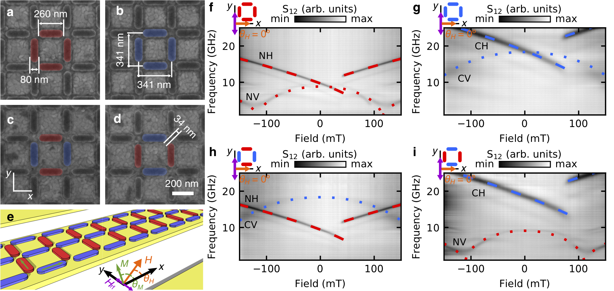
Figure 1: Characterization of single- and bicomponent artificial spin ices. Scanning electron microscopy images of studied square lattices and their dimensions for a single-component Ni₈₁Fe₁₉, b single-component Co₉₀Fe₁₀, c bicomponent Ni₈₁Fe₁₉-Co₉₀Fe₁₀ with Ni₈₁Fe₁₉ in the horizontal sublattice, and d bicomponent Ni₈₁Fe₁₉-Co₉₀Fe₁₀ with the Co₉₀Fe₁₀ in the horizontal sublattice. The red false color represents nanomagnets made of Ni₈₁Fe₁₉, and the blue false color represents nanomagnets made of Co₉₀Fe₁₀. In e, a schematic of a coplanar waveguide with a bicomponent spin ice on the signal line is shown. The corresponding absorption spectra at magnetic fields applied parallel to the signal line are shown in f–i. Horizontal elements are fitted to equation. (2): Ni₈₁Fe₁₉ modes, NH (red dash curves); Co₉₀Fe₁₀ modes, CH (blue dash curves). Vertical elements are fitted to equation (2) at high fields, and using Supplementary equation (S1.2) at low fields: Ni₈₁Fe₁₉ modes, NV (red dot curves); Co₉₀Fe₁₀ modes, CV (blue dot curves).

Results

We fabricated a set of ASI arranged in a nominally identical square geometry, but with different material combinations (see Supporting Information for details): (A) All elements consist of Ni₈₁Fe₁₉ (Fig. 1a), (B) all elements consist of Co₉₀Fe₁₀ (Fig. 1b), (C) horizontal elements are made of Ni₈₁Fe₁₉ while vertical elements are made of Co₉₀Fe₁₀ (Fig. 1c), and (D) horizontal elements are made of Co₉₀Fe₁₀, while vertical elements are made of Ni₈₁Fe₁₉ (Fig. 1d). A schematic drawing of the measurement setup is shown in Fig. 1e. We use a standard vector network analyzer (VNA) ferromagnetic resonance (FMR) technique ³⁵, see Supporting Information.

Figures 1f-i show the experimentally detected absorption spectra with an applied magnetic field parallel to the coplanar waveguide (CPW) signal line ($\theta_{H}=0^{\circ}$) as false color coded images, where a dark contrast represents maximum absorption (minimum in the transmission parameter S₁₂), while a light contrast represents minimum absorption (maximum in the transmission parameter S₁₂). The applied magnetic field in all presented measurements is swept from negative to positive field values. We can identify the main absorption lines corresponding to the different lattice sites by correlating the observed spectra with the sample configurations taking into account the magnetic properties of Ni₈₁Fe₁₉ and Co₉₀Fe₁₀.

Following the general expression given by Suhl ³⁶, the resonance frequency $f$ in an in-plane geometry is given by (see Supplementary Fig. S1 for the symbol definition):

$$f =\frac{\gamma}{2\pi}\mu_{0}\sqrt{\left[H\cos(\theta_{H}-\theta_{M})+M_{\mathrm{S}}(N_{y}-N_{x})\cos(2\theta_{M})\right]}$$

$$\quad\cdot\sqrt{\left[H\cos(\theta_{H}-\theta_{M})+M_{\mathrm{S}}\left(N_{z}-N_{x}\cos^{2}(\theta_{M})-N_{y}\sin^{2}(\theta_{M})\right)\right]}$$ (1)

where $\gamma$ is the gyromagnetic ratio, $\mu_{0}$ is the magnetic permeability, $H$ is the external magnetic field, $M_{\textrm{S}}$ the saturation magnetization, $\theta_{H,M}$ the angle between the $x$ axis and the external magnetic field and the magnetization, respectively, and $N_{x,y,z}$ the demagnetization factors along each axis. In the derivation of equation (1), we have considered a negligible magnetocrystalline anisotropy (confirmed in thin film data, shown in Supplementary Fig. S2).

In the case of a magnetic field applied along the $x$ axis, $\theta_{H}=0$, and the magnetization pointing along the magnetic field ($\theta_{M}=\theta_{H}=0$), the expression can be reduced to

$$f=\frac{\gamma}{2\pi}\mu_{0}\sqrt{[H+(N_{y}-N_{x})M_{\mathrm{S}}][H+(N_{z}-N_{x})M_{\mathrm{S}}]},$$ (2)

similar to previous results ²⁷.

For the horizontal elements, the magnetic field is applied along the easy axis, and equation (2) can be used with $N_{y}>N_{z}>N_{x}$.

For the vertical elements, the value of $\theta_{M}$ is not constant at low fields. For instance, due to the shape anisotropy, the magnetization points perpendicular to the $x$ axis ($\theta_{M}=\pi/2$) at zero field, and tilts towards the $x$ axis as the magnetic field gradually increases. When the field is strong enough, the magnetization is aligned with the external field and the $x$ axis ($\theta_{M}=0$). Hence, $\cos(\theta_{M})=H/H_{1}$, where $H_{1}\sim M_{\textrm{S}}$ is the field at which the magnetization is saturated. Once this field is reached, equation (2) applies. Due to the shape anisotropy in the vertical elements, $N_{x}>N_{y}$ and $N_{x}>N_{z}$, the resulting resonant frequency is lower than in the horizontal elements, where $N_{y}>N_{x}$ (see Supporting Information for all expressions).

We first inspect the single-component Ni₈₁Fe₁₉ network: Figure 1f shows the corresponding spectrum where two main modes originating from the vertical and the horizontal elements are observed. When the sample is saturated, the magnetic moments in the horizontal elements lie in the easy axis for $\theta_{M}=\theta_{H}=0^{\circ}$ and equation (2) applies with $N_{y}>N_{x}$ and $N_{z}\approx 0$. The horizontal Ni₈₁Fe₁₉ absorption lines start at 16.5 GHz for $-150$ mT, and decrease as the field is ramped up (labeled as NH in Fig. 1f). When a field $\mu_{0}H_{\mathrm{NiFe}}=50$ mT is reached, the magnetization of the horizontal elements switches, producing a step in the absorption frequency and a change in the sign of the slope. A fit according to equation (2) is shown as a red dashed line in Fig. 1f. For the vertical elements, the magnetic field is applied along the hard axis. The absorption lines start at 4.8 GHz for $-150$ mT (labeled as NV in Fig. 1f) and decrease down to 3.4 GHz at a field of $-123$ mT, where the magnetization configuration in the vertical elements becomes unstable and then gradually rotates from the hard ($\theta_{M}=180^{\circ}$) to the easy axis direction ($\theta_{M}=90^{\circ}$). As the field decreases and the magnetization rotates to the easy axis, the resonance frequency increases until zero field is reached producing a characteristic W-shape ^{37, 38}, which is a convenient way to qualitatively inspect the FMR spectra. This mode is symmetric around zero field and the same behavior is found at positive fields. It is important to point out that the torque exerted by the microwave magnetic field $H_{\mathrm{rf}}$ on the vertical elements becomes minimum when the magnetization lies in the easy axis parallel to $H_{\mathrm{rf}}$, which results in a gradually decreasing absorption. The red dotted curves in Fig. 1f and i have been obtained by fitting the NV mode taking into account the different behavior at high and low fields, see also Supplementary equation (S1.2).

The same general behavior is observed for the single-component Co₉₀Fe₁₀ ASI (sample B) shown in Fig. 1g. However, the resonance frequencies are pushed up in comparison to Ni₈₁Fe₁₉ due to the higher $M_{\mathrm{S}}$. In this case, the mode from the horizontal islands is labeled CH and the mode from the vertical islands CV, and the fits to the analytical expressions are shown in blue dashed and blue dotted curves, respectively. In addition, the absorption lines are noticeably broader due to the larger Gilbert damping of Co₉₀Fe₁₀ as revealed by the thin-film data (shown in Supplementary Fig. S2).

The FMR spectra observed for the two bicomponent lattices are shown in Figs. 1h and i. The spectra can be understood as a superposition of the mode structure caused by either of the two components Co₉₀Fe₁₀, Ni₈₁Fe₁₉ and the sublattice site they are occupying. For sample C (Fig. 1h) the NH mode starting at 16 GHz at $-150$ mT corresponds to the horizontal Ni₈₁Fe₁₉ elements, similar to sample A as shown in Fig. 1f, while the NV mode corresponding to the vertical Ni₈₁Fe₁₉ elements is absent. Instead, we observe the CV mode of the vertical Co₉₀Fe₁₀ islands, similar to sample B as shown in Fig. 1g. When the two materials on the different sublattice sites are exchanged, the complimentary superposition of modes is observed; see Fig. 1i.

In the following, we demonstrate the tunability of the resonant dynamics by modifying the lattice interactions. We rotate the in-plane magnetic field direction with respect to the CPW guide axis, $\theta_{H}$, which alters the magnetization configuration in the islands, and hence the interaction among them. This tuning mechanism could also be used for magnon-magnon coupling and hybridized magnonic states ^{39, 40, 41}. Besides, we will show that the altered magnetization configuration enables the enhancement of the detection sensitivity to the vertical islands.

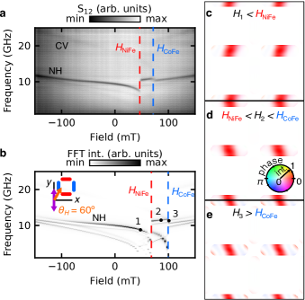
Figure 2: Results for the bicomponent sample with the Ni₈₁Fe₁₉ sublattice in the direction of the signal line with external fields applied at 60 degrees. The measured spectra are shown in a, which are in agreement with the spectra obtained in micromagnetic simulations shown in b. The profiles of the main resonant mode, NH, are shown at three representative magnetic fields marked in b: 1) Before the Ni₈₁Fe₁₉ switching (50 mT, 8.6 GHz) in c; 2) after the Ni₈₁Fe₁₉ switching and before the Co₉₀Fe₁₀ switching (80 mT, 11.6 GHz) in d; and 3) after the Co₉₀Fe₁₀ switching (100 mT, 11.5 GHz) in e. The profile plots depict the FFT intensity with the saturation (white being zero intensity, and high saturation being maximum intensity normalized to 1) and the phase as the hue, as shown in the hsv color wheel.

Figure 2 illustrates the results for sample C (Ni₈₁Fe₁₉ on the horizontal islands and Co₉₀Fe₁₀ on the vertical islands) with $\theta_{H}=60^{\circ}$. As is obvious from the experimental results, Fig. 2a, the main NH mode shifts down when $\theta_{H}$ is increased to $60^{\circ}$ (it starts at 12 GHz at $-150$ mT). With increasing field, the magnetization of the Ni₈₁Fe₁₉ islands switch at $\mu_{0}H_{\textrm{NiFe}}=47$ mT, resulting in a step-like increase in frequency and a change in sign of the slope ^{37, 38}. When the field is further increased to $\mu_{0}H_{\textrm{CoFe}}=74$ mT, the vertical Co₉₀Fe₁₀ islands switch and the NH mode shows a step-like decrease in frequency. The switching of the Co₉₀Fe₁₀ islands can also be seen in the the faint CV mode at higher frequencies. Thus, the utilization of a material with different switching field leads to emergent spin dynamics absent in single-component ASI. This method can be used to tune the dynamic response of the sublattice, making the dynamic behavior different from just the addition of the two sublattices (which manifests in the superposition of the spectra).

The results of the corresponding simulations qualitatively agree with the experimental data, as shown in Fig. 2b. The trend of the main mode NH is reproduced, as well as the steps in frequency when the different sublattices switch; first the Ni₈₁Fe₁₉ sublattice (indicated by vertical red dashed lines in Figs. 2a and b), and then the Co₉₀Fe₁₀ sublattice (indicated by vertical blue dashed lines in Figs. 2a and b). Note that the step at $\mu_{0}H_{\mathrm{CoFe}}$ is not observed in sample A, composed of only Ni₈₁Fe₁₉, as shown in Supplementary Fig. S3. The values of the resonant frequency and the switching fields do not exactly match the ones observed in the experiment, which may be caused by slightly different values of parameters used in the simulations such as saturation magnetization, geometry, and exact angle of the applied magnetic field.

In addition to the absorption spectra, we determine the excitation profiles of the lattice structures by micromagnetic simulations. In this way, we can characterize the different modes and determine the spatial location of particular excitations. Besides the spatial profile of the FFT intensity, we also obtain the phase of the oscillations, and map both the intensity and the phase using the hsv color space, where h stands for hue, s for saturation, and v for value. Here, the phase is represented by the hue and the intensity by the saturation, with the value being fixed to 1. We find that the most intense curve in Fig. 2b (labeled as NH) corresponds to oscillations coming from the center of the horizontal Ni₈₁Fe₁₉ islands. Figure 2c shows the excitation profile at point 1 in the simulation shown in Fig. 2b before the Ni₈₁Fe₁₉ islands switch. This first-order oscillation mode is characterized by an anti-node with maximum intensity in the center of the horizontal island and two nodes in the edges of the island. As the Ni₈₁Fe₁₉ islands reverse their magnetization at $\mu_{0}H_{\mathrm{NiFe}}$, the oscillation remains localized in the center of the Ni₈₁Fe₁₉ islands with the nodes staying at the edges, and a slightly opposite tilt determined by the relative orientation of the magnetization and the external field. This is depicted in Fig. 2d, corresponding to point 2 in Fig. 2b. When the vertical Co₉₀Fe₁₀ islands switch at $\mu_{0}H_{\mathrm{CoFe}}$, the frequency drops and a higher order excitation in the Ni₈₁Fe₁₉ islands replaces the fundamental mode. In this higher-order mode, the edges of the horizontal islands oscillate and two additional nodes appear between the center and the edges at each side. Between the nodes, a small, less-intense oscillation occurs out of phase, as shown in Fig. 2e (corresponding to point 3 in Fig. 2b).

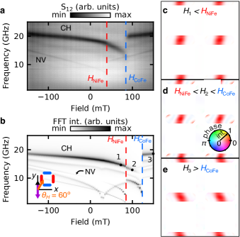
Figure 3: Results for the bicomponent sample with the Co₉₀Fe₁₀ sublattice in the direction of the signal line with external fields applied at 60 degrees. The measured spectra are shown in a, which are in agreement with the spectra obtained in micromagnetic simulations shown in b. The profiles of the main resonant mode, CH, are shown at three representative magnetic fields marked in b: 1) Before the nd the Ni₈₁Fe₁₉ switching (80 mT, 14.4 GHz) in c; 2) after the Ni₈₁Fe₁₉ switching and before the Co₉₀Fe₁₀ switching (100 mT, 12.8 GHz) in d; and 3) after the Co₉₀Fe₁₀ switching (150 mT, 18.6 GHz) in e. The profile plots depict the FFT intensity with the saturation (white being zero intensity, and high saturation being maximum intensity normalized to 1) and the phase as the hue, as shown in the hsv color wheel.

Conversely, a similar behavior can be observed in sample D, where the Co₉₀Fe₁₀ and Ni₈₁Fe₁₉ islands are exchanged, Fig. 3. In the experimental data (Fig. 3a) the Co₉₀Fe₁₀ main mode (labeled CH) from the horizontal islands shows a small step to lower frequencies at a magnetic field of $\mu_{0}H_{\mathrm{NiFe}}=39$ mT, when the vertical Ni₈₁Fe₁₉ islands switch. The NV mode from the vertical islands (faintly visible at smaller frequencies) also exhibits a step-like increase and change in sign of the slope, corroborating that it is indeed the vertical Ni₈₁Fe₁₉ islands reversing. Additionally to these indications, the small step in the CH mode is absent in the data from sample B (single-component Co₉₀Fe₁₀), see Supplementary Fig. S4. At $\mu_{0}H_{\mathrm{CoFe}}=83$ mT the horizontal Co₉₀Fe₁₀ islands reverse, resulting in a step-like increase in the CH main mode frequency and a change in sign of the slope. At the same time, we observe a small step-like decrease in the NV mode frequency. The same qualitative trends are obtained in the micromagnetic simulations shown in Fig. 3b for the CH and NV modes. The micromagnetic simulations show additional modes not obersved in the experiments, produced by higher order modes and modes localized at the edges of the samples. While these modes might be excited in our experiments, their localized nature at the ends of the islands leads to an intensity that is too small to be detected experimentally.

Similarly to the case of sample C, the most intense CH mode is due to the central regions of the horizontal islands (Fig. 3c shows the excitation profile at point 1 in Fig. 3b), before the Ni₈₁Fe₁₉ islands switch. When the Ni₈₁Fe₁₉ vertical islands switch, the frequency drops and a higher order excitation occurs, as shown in Fig. 3d, corresponding to the excitation profile at point 2 in Fig. 3b. This is analogous to the switching of the Co₉₀Fe₁₀ vertical islands in sample C. Finally, as the Co₉₀Fe₁₀ horizontal islands of sample D switch, the central oscillation region tilts slightly in the opposite direction as the magnetization aligns with the external field, as shown in Fig. 3e corresponding to the excitation profile at point 3 in Fig. 3b. The change in the tilt is in agreement with the behavior of sample C when the Ni₈₁Fe₁₉ horizontal islands switch.

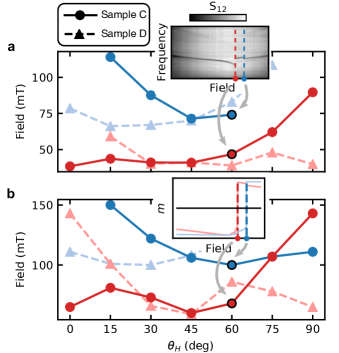
Figure 4: Angular dependence of the switching fields in the bicomponent ASIs. Change in the switching fields for sample C (dark solid lines and dots) and sample D (light dashed lines and triangles), for both the Ni₈₁Fe₁₉ sublattice (red curves) and the Co₉₀Fe₁₀ sublattice (blue curves), obtained in experiments a and simulations b. The switching fields from the experimental data in a are obtained from the dynamic measurements (as shown in the inset), and the switching fields from the simulated data in b are obtained from the simulated hysteresis loops (as shown in the inset).

Although the exact field values are different, a similar trend is observed in the switching field values obtained from experiment and simulation, as summarized in Fig. 4 as a function of the in-plane field angel $\theta_{H}$. Interchanging the sublattices from sample C to sample D results in the expected symmetric behavior around $\theta_{H}=45^{\circ}$ of the switching fields, as is apparent from the comparison between the curves for samples C and D shown in Fig. 4a. The choice of particular materials and their position on the specific lattice sites affect the intricate dynamics of the ASI. For instance, the micromagnetic simulations (Fig. 4b) show that it is possible to change which sublattice switches at lower fields by just varying the magnetic field angle. Our results show that the interaction and the dynamics can be modified by a proper choice of the materials. In contrast, in single-element lattices, the switching of both sublattices occurs at similar field values (see Supplementary Fig. S5). Thus, by using dissimilar materials, we are able to extend the region at which only one sublattice has switched while the complementary sublattice retains the original magnetization configuration, allowing for an extended region in which intermediate modes can exist.

In summary, we showed that using a bicomponent artificial spin ice arranged on a square lattice, we can finely tune the interaction between the lattice sites. We demonstrate that ferromagnetic resonance is an effective tool to probe this interaction. The resonant dynamics in the nanoscale network can be precisely adjusted by changing the magnitude and the angle of the applied magnetic field. As the islands of one sublattice switch, the dynamics of the opposite sublattice is affected due to the change in the local dipolar field distribution. Thus, the choice of materials determines the particular switching field of each sublattice, and a further adjustment can be achieved by changing the external magnetic field direction. The reported tuning mechanism of the inter- and intra-lattice interactions offers a richer manipulation of the specific mode spectra than the previously reported superposition principle of the resonant dynamics in single-component artificial spin ice. Our results demonstrate the ability to realize a novel type of two-dimensional magnonic crystals that opens the door to new concepts in nano-magnonics.

We used a dynamic FMR approach for detecting the lattice interactions and we primarily focused on harnessing the tunability of these interactions for nano-magnonics. However, we note that the choice of dissimilar materials for different sublattice sites could also be exploited for controlling the order state of artificial spin ice ^{42, 43, 33}.

1 Supporting Information

The Supporting Information contains information about the sample fabrication, VNA-FMR measurement technique, micromagnetic simulations, detailed ferromagnetic resonance equations, and additional data for reference films and single-component ASI.

This work was supported by the U.S. Department of Energy, Office of Basic Energy Sciences, Division of Materials Sciences and Engineering under Award DE-SC0020308.

References

- Kruglyak et al. 2010 Kruglyak, V. V.; Demokritov, S. O.; Grundler, D. J. Phys. D. Appl. Phys. 2010, 43, 264001
- Chumak et al. 2015 Chumak, A. V.; Vasyuchka, V. I.; Serga, A. A.; Hillebrands, B. Nat. Phys. 2015, 11, 453–461
- Vogt et al. 2014 Vogt, K.; Fradin, F.; Pearson, J.; Sebastian, T.; Bader, S.; Hillebrands, B.; Hoffmann, A.; Schultheiss, H. Nat. Commun. 2014, 5, 3727
- Bonetti and Åkerman 2013 Bonetti, S.; Åkerman, J. In Magnonics; Demokritov, S. O., Slavin, A. N., Eds.; Topics in Applied Physics; Springer Berlin Heidelberg: Berlin, Heidelberg, 2013; Vol. 125; pp 177–187
- Grollier et al. 2016 Grollier, J.; Querlioz, D.; Stiles, M. D. Proc. IEEE 2016, 104, 2024–2039
- Csaba et al. 2017 Csaba, G.; Papp, Á.; Porod, W. Physics Letters A 2017, 381, 1471–1476
- Tabuchi et al. 2014 Tabuchi, Y.; Ishino, S.; Ishikawa, T.; Yamazaki, R.; Usami, K.; Nakamura, Y. Phys. Rev. Lett. 2014, 113, 083603–5
- Zhang et al. 2016 Zhang, X.; Zou, C.-L.; Jiang, L.; Tang, H. X. Science Advances 2016, 2, e1501286
- Wang et al. 2009 Wang, Z. K.; Zhang, V. L.; Lim, H. S.; Ng, S. C.; Kuok, M. H.; Jain, S.; Adeyeye, A. O. Appl. Phys. Lett. 2009, 94, 083112
- Kostylev et al. 2008 Kostylev, M.; Schrader, P.; Stamps, R. L.; Gubbiotti, G.; Carlotti, G.; Adeyeye, A. O.; Goolaup, S.; Singh, N. Appl. Phys. Lett. 2008, 92, 132504
- Chumak et al. 2017 Chumak, A. V.; Serga, A. A.; Hillebrands, B. J. Phys. D 2017, 50, 244001
- Lenk et al. 2011 Lenk, B.; Ulrichs, H.; Garbs, F.; Münzenberg, M. Phys. Rep. 2011, 507, 107–136
- Krawczyk and Grundler 2014 Krawczyk, M.; Grundler, D. J. Phys.: Condens. Matter 2014, 26, 123202–33
- Lendinez and Jungfleisch 2020 Lendinez, S.; Jungfleisch, M. B. J. Phys. Condens. Matter 2020, 32, 013001
- Sklenar et al. 2019 Sklenar, J.; Lendinez, S.; Jungfleisch, M. B. Solid State Phys. 2019, 70, 171–235
- Skjærvø et al. 2019 Skjærvø, S. H.; Marrows, C. H.; Stamps, R. L.; Heyderman, L. J. Nat Rev Phys 2019, 439, 1–16
- Gliga et al. 2020 Gliga, S.; Iacocca, E.; Heinonen, O. G. APL Materials 2020, 8, 040911
- Dion et al. 2019 Dion, T.; Arroo, D. M.; Yamanoi, K.; Kimura, T.; Gartside, J. C.; Cohen, L. F.; Kurebayashi, H.; Branford, W. R. Phys. Rev. B 2019, 100, 054433
- Iacocca et al. 2020 Iacocca, E.; Gliga, S.; Heinonen, O. G. Phys. Rev. Applied 2020, 13, 044047
- Harris et al. 1997 Harris, M. J.; Bramwell, S. T.; McMorrow, D. F.; Zeiske, T.; Godfrey, K. W. Phys. Rev. Lett. 1997, 79, 2554–2557
- Bramwell and Gingras 2001 Bramwell, S. T.; Gingras, M. J. Science 2001, 294, 1495–501
- Branford et al. 2012 Branford, W. R.; Ladak, S.; Read, D. E.; Zeissler, K.; Cohen, L. F. Science 2012, 335, 1597–600
- Gilbert et al. 2016 Gilbert, I.; Nisoli, C.; Schiffer, P. Phys. Today 2016, 69, 54–59
- Sklenar et al. 2013 Sklenar, J.; Bhat, V. S.; DeLong, L. E.; Ketterson, J. B. J. Appl. Phys. 2013, 113, 17B530
- Gliga et al. 2013 Gliga, S.; Kákay, A.; Hertel, R.; Heinonen, O. G. Phys. Rev. Lett. 2013, 110, 117205
- Jungfleisch et al. 2016 Jungfleisch, M. B.; Zhang, W.; Iacocca, E.; Sklenar, J.; Ding, J.; Jiang, W.; Zhang, S.; Pearson, J. E.; Novosad, V.; Ketterson, J. B.; Heinonen, O.; Hoffmann, A. Phys. Rev. B 2016, 93, 100401
- Zhou et al. 2016 Zhou, X.; Chua, G.-L.; Singh, N.; Adeyeye, A. O. Adv. Funct. Mater. 2016, 26, 1437–1444
- Iacocca et al. 2016 Iacocca, E.; Gliga, S.; Stamps, R. L.; Heinonen, O. Phys. Rev. B 2016, 93, 134420
- Gubbiotti et al. 2018 Gubbiotti, G.; Zhou, X.; Haghshenasfard, Z.; Cottam, M. G.; Adeyeye, A. O. Phys. Rev. B 2018, 97, 134428
- Östman et al. 2018 Östman, E.; Stopfel, H.; Chioar, I.-A.; Arnalds, U. B.; Stein, A.; Kapaklis, V.; Hjörvarsson, B. Nat. Phys. 2018, 14, 375–379
- Drisko et al. 2017 Drisko, J.; Marsh, T.; Cumings, J. Nat. Commun. 2017, 8, 14009
- Schanilec et al. 2019 Schanilec, V.; Perrin, Y.; Denmat, S. L.; Canals, B.; Rougemaille, N. arXiv 2019, 1902.00452
- Farhan et al. 2019 Farhan, A.; Saccone, M.; Petersen, C. F.; Dhuey, S.; Chopdekar, R. V.; Huang, Y.-L.; Kent, N.; Chen, Z.; Alava, M. J.; Lippert, T.; Scholl, A.; van Dijken, S. Sci. Adv. 2019, 5, eaav6380
- Vansteenkiste et al. 2014 Vansteenkiste, A.; Leliaert, J.; Dvornik, M.; Helsen, M.; Garcia-Sanchez, F.; Van Waeyenberge, B. AIP Adv. 2014, 4, 107133
- Kalarickal et al. 2006 Kalarickal, S. S.; Krivosik, P.; Wu, M.; Patton, C. E.; Schneider, M. L.; Kabos, P.; Silva, T. J.; Nibarger, J. P. Journal of Applied Physics 2006, 99, 093909
- Suhl 1955 Suhl, H. Phys. Rev. 1955, 97, 555–557
- Montoncello et al. 2018 Montoncello, F.; Giovannini, L.; Bang, W.; Ketterson, J. B.; Jungfleisch, M. B.; Hoffmann, A.; Farmer, B. W.; De Long, L. E. Phys. Rev. B 2018, 97, 014421
- Bang et al. 2020 Bang, W.; Sturm, J.; Silvani, R.; Kaffash, M. T.; Hoffmann, A.; Ketterson, J. B.; Montoncello, F.; Jungfleisch, M. B. Phys. Rev. Applied 2020, 14, 014079
- Shiota et al. 2020 Shiota, Y.; Taniguchi, T.; Ishibashi, M.; Moriyama, T.; Ono, T. Phys. Rev. Lett. 2020, 125, 017203
- Li et al. 2020 Li, Y.; Cao, W.; Amin, V. P.; Zhang, Z.; Gibbons, J.; Sklenar, J.; Pearson, J.; Haney, P. M.; Stiles, M. D.; Bailey, W. E.; Novosad, V.; Hoffmann, A.; Zhang, W. Phys. Rev. Lett. 2020, 124, 117202
- MacNeill et al. 2019 MacNeill, D.; Hou, J. T.; Klein, D. R.; Zhang, P.; Jarillo-Herrero, P.; Liu, L. Phys. Rev. Lett. 2019, 123, 047204
- Mengotti et al. 2008 Mengotti, E.; Heyderman, L. J.; Fraile Rodríguez, A.; Bisig, A.; Le Guyader, L.; Nolting, F.; Braun, H. B. Phys. Rev. B 2008, 78, 144402
- Anghinolfi et al. 2015 Anghinolfi, L.; Luetkens, H.; Perron, J.; Flokstra, M. G.; Sendetskyi, O.; Suter, A.; Prokscha, T.; Derlet, P. M.; Lee, S. L.; Heyderman, L. J. Nat. Commun. 2015, 6, 8278