Quantum graphs -
Generic eigenfunctions and their nodal count and Neumann count statistics

In Partial Fulfillment of The

Requirements for the Degree of

Doctor of Philosophy

Lior Alon

Technion - Israel institute of Technology

Av 5780, Haifa, August 2020

 

To my mother

 

The Research Thesis Was Done Under The Supervision of

Associate Prof. Ram Band in The Faculty of Mathematics.

Some results in this thesis have been published as articles by the author together with collaborators:

1. L. Alon, R. Band, and G. Berkolaiko, Nodal statistics on quantum graphs, Communications in Mathematical Physics, (2018).

2. L. Alon, R. Band, M. Bersudsky, and S. Egger, Neumann domains on graphs and manifolds, Analysis and geometry on graphs and manifolds, 461 (2020), p.203.

The Generous Financial Help of the Technion, the Irwin and Joan Jacobs Fellowship, and the Ruth and Prof. Arigo Finzi Fellowship is Gratefully Acknowledged.

 

This dissertation is the last milestone of my Ph.D. Journey. Throughout this Journey I have received a great deal of support and assistance for which I am thankful.

I would first like to thank my Ph.D. advisor, Rami Band, for his guidance and support, for believing in me when I had doubts, and for his ability to teach me so much and in the same time acknowledge and appreciate the ideas I bring with me. Thank you Rami for your insightful and uncompromising feedback along every step of the way, you’ve helped me grow and pushed my work to higher levels.

I would also like to thank Gregory Berkolaiko, my non-formal co-advisor, colleague and friend. Thank you for your advice and thank you for always being honest and straightforward.

I would like to thank Yehuda Pinchover and Uzy Smilansky for reading and commenting on my thesis. I would also like to thank Uzy for many insightful conversations, for teaching me physics, mathematics and history all together, and most importantly, for setting the ground on which my work stands.

I would also like to thank the mathematics faculty of the Technion for being my second home in the last eight years. I would like to thank the administrative staff, and Anat in particular, for all their caring and support. I would also like to thank the faculty members, for their willingness to help, give advice, teach and discuss mathematics beyond any formal course or office hours. In particular, Amos Nevo, Uri Shapira, Dani Neftin, Orr Shalit, Ron Rosenthal, Tali Pinsky and Nir Lazarovitch.

Finally, I would like to thank my family, my father and sisters, who supported me during the hard times. I would like to thank my son, Itamar, whose arrival (two and half years ago) had given me new hopes and new purpose in life.
Last but not least, I want to thanks my wife, Adi, for her infinite support. Thank you for believing in me, and for not allowing me to stop believing in myself. Non of this would have been possible without you by my side.

This thesis is dedicated to the memory of my mother, Tami Alon, who left us eight years ago and did not get the opportunity to see me pursuing my dream.

Abstract

In this thesis, we study Laplacian eigenfunctions on metric graphs, also known as quantum graphs. We restrict the discussion to standard quantum graphs. These are finite connected metric graphs with functions that satisfy Neumann vertex conditions.

The first goal of this thesis is the study of the nodal count problem. That is the number of points on which the $n$th eigenfunction vanishes. We provide a probabilistic setting using which we are able to define the nodal count’s statistics. We show that the nodal count’s statistics admits a topological symmetry by which the first Betti number of the graph can be obtained. This result generalizes a result by which the nodal count is 0,1,2,3… if and only if the graph is a tree. We revise a conjecture that predicts a universal Gaussian behavior of the nodal count’s statistics for large graphs, and prove it for a certain family of graphs which we call ‘trees of cycles’.

The second goal is to formulate and study a new closely related counting problem which we call the Neumann count, in which one counts the number of local extrema of the $n$th eigenfunction. This counting problem is motivated by the Neumann partitions of planar domains, a novel concept in spectral geometry. We provide uniform bounds on the Neumann count and investigate the Neumann count’s statistics using our probabilistic setting. We show that the Neumann count’s statistics admits a symmetry by which the number of leafs of the graph can be obtained. In particular, we show that the Neumann count provides a complementary geometrical information to that obtained from the nodal count. We show that for a certain family of tree graphs the Neumann count’s statistics can be calculated explicitly and it approaches a Gaussian distribution for large enough graphs, similarly to the nodal count conjecture.

The third goal is a genericity result, which justifies the generality of the Neumann count discussion. To this day it was known that generically, eigenfunctions do not vanish on vertices. We generalize this result to derivatives at vertices as well. That is, generically, the derivatives of an eigenfunction on interior vertices do not vanish.

List of Symbols

$\Gamma$	A discrete graph
$\mathcal{E},\mathcal{V}$	The sets of edges and vertices of $\Gamma$
$E,V$	The number of edges and the number of vertices of $\Gamma$
$\beta$	The first Betti number of $\Gamma$
$\vec{\mathcal{E}}$	The set of directed edges of $\Gamma$
$\partial\Gamma,\mathcal{V}_{in}$	The boundary vertices (leafs) of $\Gamma$ and the set of interior vertices in $\Gamma$
$\mathcal{E}_{v}$	The set of edges connected to a vertex $v$
$\Gamma_{\vec{l}{}}$	A standard quantum graph with edge lengths $\vec{l}{}$
$L$	The total length of $\Gamma_{\vec{l}{}}$
$\partial_{e}f(v)$	The outgoing derivative of $f$ at $v$ in the direction of $e\in\mathcal{E}_{v}$
$f_{n},k_{n}$	The $n$th eigenfunction of $\Gamma_{\vec{l}{}}$ and its (square root) eigenvalue
$\mathcal{G},\mathcal{L}$	The index sets of generic eigenfunctions, and of loop-eigenfunctions
$d(A)$	The natural density of an index set $A$
$\phi(n)$	The nodal count of the $n$th eigenfunction
$\sigma(n)$	The nodal surplus of the $n$th eigenfunction, $\phi(n)-n$
$\mu(n)$	The Neumann count of the $n$th eigenfunction
$\omega(n)$	The Neumann surplus of the $n$th eigenfunction, $\mu(n)-n$
$\Omega^{v}$	The Neumann domain containing $v$
$N(\Omega)$	The spectral position of the Neumann domain $\Omega$
$\rho(\Omega)$	The wavelength capacity of the Neumann domain $\Omega$
$Eig(\Gamma_{\vec{l}{}},k^{2})$	The $k^{2}$ eigenspace of $\Gamma_{\vec{l}{}}$
$\mathbb{T}^{\mathcal{E}}$	The characteristic torus of $\Gamma$, $(\mathbb{R}/2\pi\mathbb{Z})^{\mathcal{E}}$
$\{*\}$	The quotient map from $\mathbb{R}^{\mathcal{E}}$ to $\mathbb{T}^{\mathcal{E}}$, $\{\vec{x}\}:=\vec{x}\ mod\ 2\pi$
$\Gamma_{\vec{\kappa}{}}$	The standard quantum graph associated to $\vec{\kappa}\in\mathbb{T}^{\mathcal{E}}$
$U_{\vec{\kappa}{}}$	The unitary evolution matrix associated to $\vec{\kappa}\in\mathbb{T}^{\mathcal{E}}$
$F(\vec{\kappa})$	The secular function of $\Gamma$
$\Sigma,\Sigma^{reg}$	The secular manifold of $\Gamma$ and its regular part
$f_{\vec{\kappa}{}}$	The canonical eigenfunction associated to $\vec{\kappa}\in\Sigma^{reg}$
$\mu_{\vec{l}{}}$	The Barra-Gaspard measure associated to $\vec{l}$

1. Introduction

The following thesis lies in the mathematical field of spectral geometry, but can be regarded also as a work in the field of quantum chaos. In the following section we provide the needed context for our main results. We first review the field of quantum chaos, as the motivation of our research, after which we briefly present the aspects of spectral geometry relevant to the subjects of our work: nodal count, Neumann count and genericity. We then present each subject, first describing the known results on manifolds for comparison and motivation, then known results for quantum graphs, following which we present and discuss our new result. But first, let us introduce quantum graphs.

Quantum graphs

A Quantum Graph is a model for a quantum particle on a network. Mathematically, a quantum graph is a metric graph, a 1-d simplicial complex, equipped with a differential operator (usually a Schrödinger operator). This model was introduced in the 30’s by Pauling [102] to describe free electrons of organic molecules, and was further developed in the 50’s by Ruedenberg and Scherr [110] that considered quantum graphs as an idealization of a network of wires of very small cross-section. For modern analysis of the zero cross-section limit see [108] and [64]. The list of successful applications of quantum graphs in the study of complex phenomena include superconductivity in granular and artificial materials [4], Anderson localization [11], electromagnetic waveguide networks [63, 59] and nanotechnology [65] to name but a few. The name ‘quantum graph’ was first coined in the late 90’s by Smilansky and Kottos [83] in their work on quantum chaos. Following their work and subsequent works, such as [23, 24, 29, 30], quantum graphs gained popularity as models for quantum chaos. A thorough introduction to quantum graphs and their applications can be found in the following (partial list of) reviews on the subject [33, 71, 86].

Quantum chaos

Quantum chaos is a field of research in physics that studies the relation between quantum mechanics and classical (Hamiltonian) mechanics, through the scope of chaos. For a reader not familiar with these notions, here is a brief description:

Quantum versus classical (Hamiltonian) mechanics in a nutshell:

Classical Hamiltonian mechanics, the modern description of Newtonian mechanics, describes the dynamics of one or many particles on a domain $\Omega$, for simplicity assume $\Omega$ is a domain in $\mathbb{R}^{n}$. The dynamics of a particle is described by its position $q\in\Omega$ and momentum $p\in\mathbb{R}^{n}$. The phase space, $\Omega\times\mathbb{R}^{n}$, is the space of all pairs $\left(q,p\right)$, and the physical setting is encoded in the Hamiltonian, $H\left(q,p\right)=\left\|p\right\|^{2}+V\left(q\right)$ which describes the energy of a particle at $\left(q,p\right)$. Hamilton’s equations $\frac{d}{dt}\left(q,p\right)=\left(\frac{\partial H}{\partial_{p}},-\frac{\partial H}{\partial_{q}}\right)$ describe the particle’s dynamics in phase space. In the simple case of $V\equiv 0$, the Hamiltonian is $H=\left\|p\right\|^{2}$ and so $p$ is piece-wise constant by Hamilton’s equations, with discontinuities at the boundary.

In quantum mechanics, the phase space $\Omega\times\mathbb{R}^{n}$ is replaced by the Hilbert space $L^{2}\left(\Omega\right)$, and the pair $\left(q,p\right)$ is replaced by a wave-function $f\in L^{2}\left(\Omega\right)$. The position and momentum of the particle are no longer deterministic and are given on average by $\left\langle\boldsymbol{q}\right\rangle=\left\langle f,\boldsymbol{q}f\right\rangle$ and $\left\langle\boldsymbol{p}\right\rangle=\left\langle f,\boldsymbol{p}f\right\rangle$. Where $\left\langle*,*\right\rangle$ denotes the $L^{2}$ inner product, $\boldsymbol{q}$ is a multiplicative operator and $\boldsymbol{p}=i\hbar\nabla$ is the derivative operator scaled by a constant $\hbar$. The classical Hamiltonian $H\left(p,q\right)$ is upgraded to a self-adjoint differential operator $\boldsymbol{H}=H\left(\boldsymbol{q},\boldsymbol{p}\right)$. In particular the term $\left\|p\right\|^{2}$ is upgraded to the (positive) rescaled Laplacian $\hbar^{2}\Delta$. In general, the operators $\boldsymbol{q}$, $\boldsymbol{p}$ and $\boldsymbol{H}$ are unbounded and one should specify the domain $D_{\boldsymbol{H}}\subset L^{2}\left(\Omega\right)$ on which $\boldsymbol{H}$ is (weakly) defined and is self-adjoint. The dynamics of the wave-function, namely the time evolution of a wave function $f_{t}$ at time $t\in\mathbb{R}$, is according to Schrödinger’s equation $i\hbar\frac{d}{dt}f_{t}=\boldsymbol{H}f_{t}$. A standard separation of variables usually reduce the problem to the “stationary Schrödinger’s equation” $\boldsymbol{H}f=\lambda f$.

Classical chaos:

A standard classification of classical systems distinguishes between chaotic and integrable systems. Systems where certain symmetries and constants of motion can reduce the number of degrees of freedom are called integrable. From a dynamical point of view, a system is integrable if it has a maximal number of integrals of motion such that the phase space can be foliated by the level sets of $H$ and the integrals of motion. Chaotic systems are, in a sense, as far from integrable as possible. These are systems with dense trajectories in phase space, which are extremely sensitive to perturbations. That is, the distance between two close trajectories grows exponentially with time. Chaotic systems are very hard to investigate, thus in the study of chaos even the simplest systems that can exhibit chaotic behavior are of interest. A simple study case of chaotic behavior is that of billiard domains: A free particle ( $H=\left\|p\right\|^{2}$) on a compact planar domain $\Omega$, that bounces (symmetrically) when hitting the boundary. The classification of a billiard as integrable or chaotic is dictated by the shape of $\Omega$. Rectangles and ellipses are integrable, but “simple” chaotic billiards can be constructed, for example Sinai’s billiard, a square with a round hole in the middle.

Quantum chaos:

The starting point of quantum chaos is the quantum (miss) behavior of systems that are classically chaotic. Einstein’s Theory of Special Relativity, in the limit of $c\rightarrow\infty$, provides the same predictions as classical Newtonian mechanics. One should expect the same from a Quantum Mechanics Theory. In the beginning of the formalizing process of Quantum Mechanics, Bohr introduced the correspondence principle, stating that at a certain scale, the Quantum Mechanics predictions should agree with the classical mechanics predictions. After Schrödinger’s probabilistic formalism of Quantum Mechanics was introduced, the correspondence principle was reformulated to state that in the $\hbar\rightarrow 0$ limit the quantum expected values of position and momentum should behave according to the classical mechanics predictions. However, unlike Special Relativity, it appears that the quantum dynamics predictions may not converge to the classical predictions, in the $\hbar\rightarrow 0$ limit, if the system is classically chaotic. For example, consider the phase-space trajectories $\left(q(t),p(t)\right)$ which governs the chaotic behaviour. The quantum expected values of position and momentum, $\left\langle\boldsymbol{q}\right\rangle$ and $\left\langle\boldsymbol{p}\right\rangle$, have widths of uncertainty $\delta\boldsymbol{q}$ and $\delta\boldsymbol{p}$ which obey the uncertainty principle $\delta\boldsymbol{q}\delta\boldsymbol{p}\geq\hbar$. Due to the uncertainty constrain, different trajectories of quantum expected values cannot be distinguished if the spacing between them is of order much smaller than $\hbar$ and so chaos in its classical sense loses its meaning. It is believed that this fundamental problem of correspondence can shed light on the very nature of Quantum Mechanics. The $\hbar\rightarrow 0$ limit of a quantum system is called semi-classical limit.

One definition for quantum chaos was presented in the Bakerian lecture 1987 by M.V. Berry [41]:

Definition: “Quantum chaology is the study of semiclassical, but nonclassical, behaviour characteristic of systems whose classical motion exhibits chaos.”

These “behavior characteristics” that we wish to study are properties of high eigenvalues and their eigenfunctions (to capture the semiclassical regime where $\hbar\ll 1$) that can distinguish chaotic from integrable. It is believed that such properties should be universal, namely, insensitive to the details of the specific system. The most famous example of such a property is spectral statistics, the statistical behavior of fluctuations of eigenvalues $\lambda_{n}$ around their asymptotic growth predicted by Weyl’s law. For example, in planar domains the asymptotic growth is linear $\lambda_{n}\sim\frac{4\pi}{\left|\Omega\right|}n$. The spectral statistics behave differently for integrable systems and chaotic systems. It was proven in 1977 by Berry and Tabor [42] that the spectrum of an integrable system has level spacing statistics corresponding to a Poisson process. The chaotic case, by nature, is much harder to analyze. The famous BGS conjecture by Bohigas, Giannoni and Schmidt [45] (which followed a nuclear physics folklore), states that the spectral statistics of chaotic systems can be predicted by the spectral statistics of a corresponding random matrix ensemble. This conjecture was a significant milestone in the field of Random matrix theory (RMT). The BGS conjecture was affirmed numerically in many chaotic models, together with related works that provided analytical supporting evidences. See [120] for a 2016 overview. It is now widely accepted that RMT spectral statistics is an indication for quantum chaos.

Quantum chaos on quantum graphs

Kottos and Smilansky [83] provided numerical evidence for RMT spectral statistics in quantum graphs with edge lengths linearly independent over $\mathbb{Q}$ (we call them rationally independent). This was the first evidence for “chaotic fingerprints” in quantum graphs. They also provided an exact trace formula for quantum graphs, similar in nature to Gutzwiller’s trace formula. Gutzwiller’s trace formula [76] (following the works of Weyl, Selberg, Krein and Schwinger) is the main tool relating the spectrum of a quantum system to periodic orbits in the classical phase space. It is an approximation of the spectral density of a quantum system in the semmiclassical limit by means of the Hamiltonian action on periodic orbits. Unlike Gutzwiller’s trace formula which has an error term that vanishes in the $\hbar\rightarrow 0$ limit, the quantum graph’s trace formula is exact without error terms. It is now a common belief that a single (finite) quantum graph is not enough to properly model quantum chaos, but in the limit of large graphs, it is a good paradigm for quantum chaos. Barra and Gaspard [23] provided an implicit analytic formula for the level spacing distribution of quantum graphs with rationally independent edge lengths. Their work shows that the statistics of a single graph has a small but not neglectable deviation from the RMT statistics. However, they noticed, numerically, that this deviation was independent of the choice of edge lengths (under the rationality condition) and that the deviation decreases as the graph grows. Further works on quantum chaos on quantum graphs are [29, 30, 31, 69, 71, 81] for example.

Another behavior characteristic of chaos in quantum graphs, suggested by [73], is the nodal statistics. This is the subject of our work [8]. To elaborate, let us first introduce the nodal count problem from the scope of spectral geometry.

Spectral geometry

Spectral geometry aims to study the relations between spectral properties of differential operators (usually the Laplacian) and the geometric structure of the space on which they act (usually a Riemannian manifold). The term “spectral properties” is not confined to properties of the spectrum alone, but also to the “landscape” of eigenfunctions. A popular theme of spectral geometry is inverse problems. That is, what geometrical information can be recovered from spectral properties. Such a question was famously popularized by Mark Kac, asking ‘Can one hear the shape of a drum?’ in [80]. While Milnor provided a counter example for isospectral sixteen dimensional manifolds in [95], the question for planar domains held open for three decades until 1992 when a counter example of isospectral planar domains was found by Gordon, Webb and Wolpert in [74] based on ideas from Sunada’s theory [117]. Classifying planar domains that have unique spectrum is still an active topic, with recent works to this day such as [78]. A 2014 survey is found in [126]. It was only natural to look for other spectral properties, those related to the “landscape” of eigenfunctions, to resolve isospectrality. Smilansky, Gnutzmann and Sondergaard conjectured in [72] that the nodal count (which will be presented next) would resolve isospectrality for planar domains. In a following work of Gnutzmann and Smilansky with Karageorge [70], a nodal count “trace formula” is provided for certain families of planar domains, using which one can reconstruct these drums. It was affirmed that the nodal count can solve isospectrality in certain settings, as seen in [51, 49] for example, but counter examples were given in [50], and the general validity of this conjecture is still open.

Isospectrality on quantum graphs

The isospectral problem is a good example for a quantum graphs problem arising from manifolds and planar domains. The question ‘can one hear the shape of a graph?’ was asked by Gutkin and Smilansky in [75]. They showed that any simple graph with rationally independent edge lengths has a unique spectrum. The meaning of such result is that generically “one can hear the shape of a graph”. They also provided an algorithm to reconstruct such graphs from their spectrum, and gave a counter example of isospectral quantum graphs that do not have rationally independent edge lengths. This work led to construct more isospectral graphs [20, 21, 101] together with a generalization of Sunada’s method to graphs. The conjecture raised in [72] and the work in [70] on the resolution of isospectrality by the nodal count led to similar works on quantum graphs. It was affirmed under certain settings [19, 21, 22, 99] but counter examples were given in [100, 79], and the general validity of this conjecture is still open. In this thesis we prove that the first Betti number of a graph (a topological characterization) can be obtained from its nodal count sequence (a result from [8]). In particular, this result implies that graphs of different Betti number can be distinguished by their nodal count.

Nodal count

Given an eigenfunction of a manifold or a planar domain $\Omega$, the nodal partition is a partition of $\Omega$ according to the nodal lines (the zero set) of the eigenfunction. The nodal domains are the connected components of this partition, and are the largest connected subdomains on which the eigenfunction has a fixed sign. The nodal count, is the number of nodal domains. Given a sequence of eigenfunctions $\left\{f_{n}\right\}_{n\in\mathbb{N}}$ that span $L^{2}\left(\Omega\right)$, arranged according to their eigenvalues, we obtain a nodal count sequence. We denote the nodal count of $f_{n}$ by $\phi\left(n\right)$. The works of Albert [3, 2] and Uhlenbeck [119] assures that generically, nodal lines (zero sets) of eigenfunctions are of co-dimension one and therefore partition $\Omega$. Uhlenbeck also showed that eigenvalues are generically simple. Therefore the nodal count sequence, generically, is well defined and independent of the choice of basis. The motivation for nodal count goes back to physical experiments from the 17th century, done by DaVinci [93], Galileo [68] and Hooke [107], later to be further developed by Chladni [55] in the 18th century (probably using his skills both as a physicist and a musician). In what is now known as “Chladni figures” the vibration patterns of sound waves are visualized by spreading sand on a brass plate which is then brought to different resonances using a violin bow. The sand accumulates into the non-vibrating parts of the plate, forming the figure of the nodal lines.

In dimension one, Sturm’s oscillation theorem [116] states that $f_{n}$ will have $n-1$ nodal points (zeros). The first generalization of nodal count to planar domains and manifolds was done by Courant [58] in 1923. The famous Courant bound is $\phi\left(n\right)\leq n$. The problem of whether there are eigenfunctions for which $\phi\left(n\right)=n$ was addressed by Pleijel who showed that $\phi\left(n\right)=n$ can occur only finitely many times, by proving that $\limsup_{n\rightarrow\infty}\frac{\phi\left(n\right)}{n}\leq c<1$ in [103]. This asymptotic bound is known as Pleijel’s bound, where $c\approx 0.691...$ is given explicitly in terms of the first zero of the zeroth Bessel function. Bourgain and Steinerberger [47, 114] showed that $c$ is not optimal (improving the bound by order of $10^{-9}$). More Pleijel-like bounds can be found in [106, 90, 54].

Both Courant’s bound and Pleijel’s bound, together with many other results on nodal count, are based on the following observation. If $f$ is an eigenfunction on $\Omega$ with eigenvalue $\lambda$ and its nodal domain are denoted by $\left\{\Omega_{j}\right\}_{j=1}^{N}$, then the restriction $f|_{\Omega_{j}}$ to a nodal domain $\Omega_{j}$ is the first eigenfunction of the Dirichlet problem on $\Omega_{j}$. In particular if $\lambda_{1}\left(\Omega_{j}\right)$ denotes the first Dirichlet eigenvalue of $\Omega_{j}$, then $\lambda_{1}\left(\Omega_{j}\right)=\lambda$ for all $j$. This is a special property of the nodal partition of an eigenfunction. A variational characterization of nodal partitions was given in [10, 46, 77]. They considered all partitions of $\Omega$ into $N$ subdomains $\left\{\Omega_{j}\right\}_{j=1}^{N}$ and considered $\lambda=\max_{j}\lambda_{1}\left(\Omega_{j}\right)$ as a functional over these partitions. It appeared that the nodal partitions were critical points of $\lambda$, and minimum in the case of $\phi\left(n\right)=n$. This result led to a characterization of $\phi\left(n\right)-n$, called nodal deficiency, as a Morse index of the functional $\lambda$ under certain variations [34].

The number of nodal domains, is not the only generalization of Sturm’s oscillations to higher dimensions. Another generalization of the “number of zeros” for a $d$ dimensional manifold is $\mathcal{H}^{d-1}\left(f^{-1}\left(0\right)\right)$, the $d-1$ dimensional Hausdorff measure of the nodal set of an eigenfunction $f$. S.T. Yau famously conjectured that $c\sqrt{\lambda}\leq\mathcal{H}^{d-1}\left(f^{-1}\left(0\right)\right)\leq C\sqrt{\lambda}$ for any eigenfunction $f$ of eigenvalue $\lambda$ with some system dependent constants $c,C$. Yau’s conjecture was affirmed for real analytic manifolds by [60] and the upper bound was later upgraded to smooth manifolds by Lagunov [91] (see [92] for a recent review by Logunov and Malinnikova).

Nodal statistics - According to Courant’s bound, the normalized nodal count is bounded by $\frac{\phi\left(n\right)}{n}\leq 1$ and is asymptotically bounded by Pleijel’s bound. It was shown numerically by Blum, Gnutzmann and Smilansky in [43], that the statistics of $\frac{\phi\left(n\right)}{n}$ can distinguish between chaotic and integrable planar domains and obeys a universal behavior. Moreover, for integrable planar domains they proved that the $\frac{\phi\left(n\right)}{n}$ statistics is well defined and calculated its universal characteristics. However, for chaotic domains the numerics predict a concentration of measure at a single value. It appears numerically to have a universal Gaussian concentration with variance of order $\frac{1}{n}$. The problem of well-posedness of the statistics in the chaotic setting, not to mention proving the universal behavior, is still open. One may call it the nodal BGS conjecture as it also deals with a spectral property of chaotic systems, like the BGS conjecture, and it agrees with the initials of the authors [43]. There were several related works on the nodal count of a random eigenfunction that are believed to describe the nodal statistics. Bogomolny and Schmidt developed a percolation model for the nodal count of random eigenfunctions for which the conjectured chaotic nodal count behavior is obtained [44]. The credibility of the percolation model as a prediction for nodal count is discussed in [25]. Another important work on the nodal count of a random eigenfunction was done by Sodin and Nazarov in [97] for a random eigenfunction on a sphere based on Berry’s random wave model. In a recent work of Sodin and Nazarov [98] yet to be published, they improved their result using methods that resemble Bogomolny and Schmidt’s model. The work in [97] opened the door for many works in the area, such as the statistics of the total length of the nodal lines, $\mathcal{H}^{d-1}\left(f^{-1}\left(0\right)\right)$ for $d=2$ [123, 124, 111, 48]. In [85, 52] it was shown that the nodal length statistics for random eigenfunctions on the torus do not satisfy a universal behavior.

Nodal count on quantum graphs

Nodal count on quantum graphs first appeared in the work of Al-Obeid [1], treating only tree graphs. A decade later, independently, Gnutzmann, Smilansky and Weber raised the question of “nodal counting on quantum graphs” (for all graphs) in [73]. The context of their work was the nodal BGS conjecture, after quantum graphs were established as good paradigms for quantum chaos [75]. The conjecture that the nodal count can resolve isospectrality [72], led to a sequence of works on nodal count for quantum graphs after quantum graphs’ isospectrality was introduced [75, 26]. This conjecture was affirmed for quantum graphs in certain settings [22, 99, 19, 21] but counter examples were given in [100], and the general validity of the conjecture is still open. A particular study case in this research are tree graphs. It was shown in [1, 104, 105], and independently in [112], that Strum’s result holds for trees, and hence all trees have the same nodal count. In addition, Band proved in [12] that Sturm’s result does not hold for any other graph and therefore the nodal count distinguishes between trees and the rest of the graphs.

The nodal count for quantum graphs can be defined either as the number of nodal domains (as in the manifolds settings) or as the number of nodal points (as in Sturm’s theorem). These two counts differ by a constant for all but finitely many eigenfunctions and hence share the same statistics. Our convention is the number of nodal points, $\phi\left(n\right):=\left|f_{n}^{-1}\left(0\right)\right|$ (where the numbering of eigenfunctions starts from $n=0$ for the constant eigenfunction). The nodal count $\phi\left(n\right)$ is well defined under the assumption that $f_{n}$ does not vanish on vertices and its eigenvalue $\lambda_{n}$ is simple. This assumption was shown in [36] to hold generically. A Courant like upper bound on $\phi\left(n\right)$ was proven in [73] and a lower bound for trees was found in [112, 104, 105, 1] and later generalized to every graph by Berkolaiko in [27]. Altogether, we get the following bounds:

(1.1) $$n\leq\phi\left(n\right)\leq n+\beta,$$

where $\beta$ is the first Betti number of the graph. The non-negative deviation of $\phi\left(n\right)$ from its linear growth is called the nodal surplus, $\sigma\left(n\right):=\phi\left(n\right)-n$, and it fully characterize the nodal count. A variational characterization of $\phi\left(n\right)-n$ for quantum graphs was shown in [14] in analog to the planar domains result [34]. A similar work for discrete graphs [37] led to the nodal-magnetic work of Berkolaiko in [28]. He showed, for discrete graphs, that the analog of $\phi\left(n\right)-n$ is equal to the Morse index of the $n$th eigenvalue with respect to magnetic perturbations. A complementary work was done by Colin de Verdière in [56]. This relation, called the nodal magnetic relation, was later upgraded to quantum graphs by Berkolaiko and Weyand [39]. We will discuss it in Section 8. The nodal magnetic relation was a key ingredient in [12] and plays an important role in our works in [8] and [7]. It also provides a different physical motivation for nodal statistics from a “solid state physics” point of view, as seen in [13].

The behavior of the nodal surplus already appears in [73], one of the first nodal count works on quantum graphs, where the number of nodal domains, $\nu_{n}$, was investigated. For large enough $n$, $\nu_{n}$ and $\phi\left(n\right)$ are related by $\nu_{n}=\phi\left(n\right)-\beta+1$. Gnutzmann, Smilansky and Weber showed in [73] that $\nu_{n}-n$ is bounded in some fixed interval and considered the distribution of $\nu_{n}-n$ in this interval, which is the nodal surplus distribution (up to a constant). They raised the following quantum graphs’ nodal statistics conjecture:

Conjecture.

[73] “For well connected graphs, with incommensurate bond lengths, the distribution of the number of nodal domains in the interval mentioned above approaches a Gaussian distribution in the limit when the number of vertices is large”.

Where by ‘incommensurate bond lengths’ they mean edge lengths which are linearly independent over the rationals. We will use the name rationally independent edge lengths. The term ‘well connected graphs’ is not classified in their paper and so an important observation should be made. The limit of large graphs should be taken as $\beta\rightarrow\infty$ since (1.1) implies that $\sigma\left(n\right)\in\left\{0,1,...\beta\right\}$. In particular, as showed in [112], tree graphs (defined by $\beta=0$) have $\sigma\left(n\right)\equiv 0$ which clearly does not obey a Gaussian limit.

New results on the nodal statistics for quantum graphs

The main nodal statistics results of this thesis, which appear in [8], set the mathematical well-posedness of quantum graphs’ nodal statistics and prove the Gaussian limit conjecture for a certain family of graphs. The well-posedness will be shown in Section 6, Theorem 6.5, where we prove that nodal statistics is well defined when the edge lengths are rationally independent. That is, we prove that the following limit exists for every $j\in\left\{0,1,...\beta\right\}$,

$$p_{j}=\lim_{N\rightarrow\infty}\frac{\left\{n\leq N\,\,:\,\,\sigma\left(n\right)=j\right\}}{N}.$$

We also prove that there is a common symmetry $p_{j}=p_{\beta-j}$ for all graphs, and so the excepted value is $\mathbb{E\left(\sigma\right)=}\frac{\beta}{2}$. This result can be considered as a generalization of Band’s result for trees, showing that the nodal count distinguishes between graphs of different Betti number $\beta$.

In Section 9, Theorem 9.3, we present a family of graphs which we call trees of cycles for which the nodal statistics can be explicitly calculated and shown to have binomial distribution $\sigma\sim Bin\left(\frac{1}{2},\beta\right)$. The Gaussian limit at $\beta\rightarrow\infty$ follows, together with the variance estimate $Var\left(\sigma\right)=\frac{\beta}{4}$. Our modification to the conjecture of Gnutzmann, Smilansky and Weber is thus:

Conjecture.

[7] The nodal surplus distribution for a quantum graph, with rationally independent edge lengths and first Betti number $\beta$, approaches a Gaussian distribution in the limit of $\beta\rightarrow\infty$ as follows:

$$\frac{\sigma-\frac{\beta}{2}}{\sqrt{\mathrm{Var}\left(\sigma\right)}}\xrightarrow[\beta\rightarrow\infty]{\mathcal{D}}N\left(0,1\right).$$

Where the convergence above is in distribution and the variance is of order $\mathrm{Var}\left(\sigma\right)=\mathcal{O}\left(\beta\right)$.

In a work in progress [7] we prove this conjecture for several other families of graphs, different than the ones in [8], together with a vast numerical evidence.

Neumann count

It was first noticed by Stern in her Ph.D. thesis in 1925, that there can be arbitrarily large eigenvalues with nodal domains as small as $\phi\left(n\right)=2$ [115]. This counter intuitive fact is unavoidable. As shown by Uhlenbeck in [119], a crossing of nodal lines is unstable and can be omitted by “as small as we want” perturbations. Nodal partitions are determined by such crossings and are therefore usually unstable.

A novel idea of a more stable partition, which reflects the topography of an eigenfunction, was first suggested by Zelditch in a paragraph in [125], and (independently) was studied by McDonald and Fulling in [94]. The partition, now called Neumann partition, is the Morse-Smale complex (see [61]) of a planar domain or a 2d manifold according to a given eigenfunction $f$. A description of such partition, following the definitions and notations of [17], is as follows. Let $M$ be a 2d manifold (for simplicity assume no boundary) and let $f$ be an eigenfunction of $M$. Consider the gradient $\nabla f$ as a vector field on $M$ and consider gradient flow lines $\varphi:\mathbb{R}\rightarrow M$ such that $\frac{d}{dt}\varphi\left(t\right)=\nabla f\left(\varphi\left(t\right)\right)$. It is not hard to deduce that each gradient flow line start and ends at critical points of $f$ and that these flow lines cover $M$. The naive picture one should have in mind is that each point $x\in M$ which is not a critical point of $f$ lies on a unique gradient flow line that starts from a local minimum $q$ and ends at a local maximum $p$. This is not necessarily the case, in general, and so the discussion is restricted to eigenfunctions which are Morse, which is a generic property [119]. An eigenfunction is said to be Morse if its set of critical points is discrete and each critical point is non-degenerate (i.e Hessian of full rank).

Given a Morse eigenfunction $f$, every pair of a local minimum $q$ and a local maximum $p$ define a Neumann domain $\Omega_{p,q}$ as the union (possibly empty) of gradient flow lines of $f$ going from $p$ to $q$. On the boundary of a Neumann domain are the Neumann lines, gradient flow lines that go through a saddle point. The Neumann partition is the partition of $M$ into Neumann domains. Such a partition can be shown to be stable under small perturbations of $f$ or of the metric on $M$. Heuristically, the Neumann partition is changed only if critical points meet\appear\disappear, which generically does not happen under small enough perturbations.

A main feature of the Neumann partition and the origin of its name is that the restriction $f|_{\Omega}$ to a Neumann domain $\Omega$ is an eigenfunction of $\Omega$ with Neumann boundary conditions [16]. It is analogous to the known fact that the restriction to a nodal domain is a Dirichlet eigenfunction of that domain. However, unlike the restriction to a nodal domain, where the eigenfunction is known to be the first Dirichlet eigenfunction of that domain, for a Neumann domain this is not the case. The spectral position $N\left(\Omega\right)$ of a Neumann domain $\Omega$ of $f$ with eigenvalue $\lambda$ is the position of $\lambda$ in the spectrum of $\Omega$. Namely, the number of eigenvalues of $\Omega$ (with Neumann boundary conditions) smaller than $\lambda$. It was previously believed that like in the case of nodal domains, $N\left(\Omega\right)$ should be one, or at least very low, but the works of [17, 16] show , counter intuitively, that $N\left(\Omega\right)$ can be as high as we wish, even for simple cases like the flat torus. In analogy to the nodal count problem, the Neumann count, $\mu\left(n\right)$ is defined as the number of Neumann domains of $f_{n}$, the $n^{th}$ eigenfunction. It was shown in [17] that $\mu\left(n\right)\geq\frac{1}{2}\phi\left(n\right)$ but it is still unknown whether the Neumann count holds more geometric information on the manifold than the nodal count. In particular, Neumann statistics properties and resolution of isospectrality are still unknown in general. For more information see the review paper [9].

New results on Neumann count and statistics for quantum graphs

The novel study of Neumann partitions led naturally to the question of a Neumann partition on a quantum graph. We raised this question in [9] and compared between properties of Neumann partitions on quantum graphs and manifolds. The wealth of questions on Neumann partitions, Neumann domains and Neumann count on quantum graphs was further studied in [6]. In analogy to nodal points, the Neumann points of an eigenfunction $f$ on a quantum graph are the interior critical points (which are either local minima or maxima). The Neumann count $\mu\left(n\right)$ for a quantum graph is the number of Neumann points of $f_{n}$, the $n^{th}$ eigenfunction, and it is convenient to discuss the deviation $\omega\left(n\right)=\mu\left(n\right)-n$, called the Neumann surplus in analogy to the nodal surplus (although it can be negative). The Neumann surplus was bounded uniformly in [9, 6], in analogy to the nodal surplus bounds (1.1).

The main results of this thesis in the context of Neumann count and statistics were obtained in [6]. In Section 6, Theorem 6.5, we prove, alongside the nodal statistics, that Neumann statistics (that is the statistics of the Neumann surplus) is well defined, by existence of the limits,

$$p_{j}=\lim_{N\rightarrow\infty}\frac{\left\{n\leq N\,\,:\,\,\omega\left(n\right)=j\right\}}{N},$$

for all possible values of the Neumann surplus. We also prove a symmetry, similar to that of the nodal statistics, which provides the expected value $\mathbb{E}\left(\omega\right)=\frac{\beta-\left|\partial\Gamma\right|}{2}$, where $\left|\partial\Gamma\right|$ is the number of vertices of degree one in the graph. As a consequence, we can recover both $\beta$ and $\left|\partial\Gamma\right|$ from $\mathbb{E}\left(\omega\right)$ and $\mathbb{E}\left(\sigma\right)$. This is a major improvement to the inverse problem of the nodal count, as the number of (discrete) graphs with fixed $\beta$ and $\left|\partial\Gamma\right|$ is finite. This also proves that the nodal count and the Neumann count cannot be obtained one from the other. The question of how correlated are the nodal statistics and the Neumann statistics is discussed in [6] and is still open. In Section 9, Theorem 9.3, we prove, alongside the binomial nodal statistics of a certain family of graphs, that tree graphs whose interior vertices (those of degree larger than one) are of degree 3 have a shifted binomial Neumann statistics:

$$\omega+\left|\mathcal{V}_{in}\right|+1\sim Bin\left(\left|\mathcal{V}_{in}\right|,\frac{1}{2}\right).$$

Where $\left|\mathcal{V}_{in}\right|$ is the number of internal vertices. A Gaussian limit at $\left|\mathcal{V}_{in}\right|\rightarrow\infty$ appears here, and the universality of this limit for other families of graphs is currently investigated.

Generic properties of eigenfunctions on quantum graphs

As already stated, Uhlenbeck’s seminal work “generic properties of eigenfunctions” [119] was needed in order to discuss and define the nodal and Neumann counts on manifolds. In fact this work is crucial for almost every spectral property, as in the words of Uhlenbeck, it “set up machinery to consider the eigenfunctions of curves of operators…suggest an approach to the problem of characterizing the $n$th eigenfunction of a family of operators”. As metric graphs are not manifolds, the results of Uhlenbeck do not apply and new machinery is needed. The first genericity result for quantum graphs was obtained by Friedlander [67], who showed that for any graph structure not homeomorphic to a cycle, there is a residual set of edge lengths for which every eigenvalue of the quantum graph is simple. A decade later, Berkolaiko and Liu had found [36] that for graphs without loops (an edge connecting a vertex to itself) and a generic choice of edge lengths (in the sense of [67]) none of the eigenfunctions vanish on a vertex. This property is needed to define nodal count, and is also crucial for the nodal magnetic connection as seen in [39].

In the case where a graph has a loop, for any choice of edge lengths, there will be infinitely many eigenfunctions supported on that loop. Nevertheless, it is proven in [36], that for a generic choice of edge lengths, every eigenfunction not supported on a loop, does not vanish on any vertex. In [8] we show that the implicit generic choice of edge lengths can be replaced by the explicit restriction to rationally independent edge lengths, at the cost of a density zero sequence. Namely, for almost every eigenfunction (a density one sequence), the eigenvalue is simple and either the eigenfunction is supported on a loop or it does not vanish on any vertex.

New genericity results for quantum graphs

The main genericity result in this thesis, a work from [5] yet to be published, is that generically the derivatives of an eigenfunction do not vanish on any interior vertex (that is any vertex which is not of degree one). Here, by generically we mean either in the sense of every eigenfunction for a residual set of edge lengths, or in the sense of a density one sequence of eigenfunction for any choice of rationally independent edge lengths. We also prove that the two choices of genericity are equivalent in this case. This additional property, is needed in order to define the Neumann count and statistics.

1.1. The structure of the thesis

This thesis incorporates the nodal statistics works of [8] together with the Neumann count and statistics works of [6, 9]. The structure of the thesis and the partition into “Neumann” results of [6, 9] versus “nodal” results of [8] is illustrated in the diagram in Figure 1.1. Section 3 is a short section in which we present a uniform bound on the Neumann surplus. Section 4 is the core of this thesis, in it we present the secular manifold and provide the needed machinery for statistical investigation of eigenfunctions. A new result presented in this section is a generalization of a result from [36] on the number of connected components of the secular manifold. Section 5 is devoted to the generalization of the genericity result in [36]. The extended generic properties from this work are needed in order to define the Neumann count. In Section 6 we prove existence and symmetry of both the nodal surplus distribution (a main result of [8]) and the Neumann surplus distribution (a main result of [6]). In Section 9, we present families of graphs for which we can prove that the nodal\Neumann surplus distributions are binomials and converge to a Gaussian limit as conjectured. These results were obtained in [8] for the “nodal” case and in [6] for the Neumann “case”. Both results make use of statistical behavior of “local” properties, which are described in Sections 7 and 8. In Section 7 we present local properties of Neumann domains, providing both bounds and statistical analysis as done in [6, 9]. In Section 8 we present a brief introduction to the nodal magnetic connection that was proved in [39]. Using the nodal magnetic theorem we prove, as in [8], that the nodal surplus is given by a sum of local magnetic stability indices and analyze their statistics.

Figure 1.1. A diagram of the thesis structure. The arrows indicate dependence. Sections 5,6 and 9 in bold as these hold the main results (although new results appear in every chapter from 4 to 9). The ’Neumann’ (or ’nodal’) block indicates results that appear in [6] (or [8]).

2. Preliminaries

2.1. Basic graph definitions and notations

Throughout this manuscript, the graphs we consider are finite and connected. We denote by $\mathcal{V}$ the set of the graph vertices and by $\mathcal{E}$ the set of its edges. We denote their cardinality by $V:=\left|\mathcal{V}\right|$ and $E:=\left|\mathcal{E}\right|$. Our discussion is not restricted to simple graphs. Namely, two vertices may be connected by more than one edge and it is also possible for an edge to connect a vertex to itself. An edge connecting a vertex to itself is called a loop. Given a vertex $v\in\mathcal{V}$ we denote the multi-set of edges connected to $v$ by $\mathcal{E}_{v}$. We note that every loop connected to $v$ will appear twice in $\mathcal{E}_{v}$. The degree of a vertex is denoted by $\mathrm{deg}(v):=\left|\mathcal{E}_{v}\right|$.

Remark 2.1.

Throughout this manuscript we assume no $\mathrm{deg}(v)=2$ vertices and that $E>1$.

We will show in Remark 2.14 why adding\removing vertices of $\mathrm{deg}(v)=2$ does not affect the quantum graphs we discuss. The restriction to $E>1$, is to exclude the loop graph which is the only exception in most of the following theorems (as it has a continuous symmetry which gives a completely non-simple spectrum). By considering $E>1$ we also exclude the interval, which is fully analyzed in the famous works of Sturm and Liouville.

Definition 2.2.

We call a vertex of degree one, a boundary vertex, and define the boundary of the graph as $\partial\Gamma:=\left\{v\in\mathcal{V}\thinspace|\,\mathrm{deg}(v)=1\right\}.$ The rest of the vertices are called interior vertices and we denote the set of interior vertices by $\mathcal{V}_{in}:=\mathcal{V}\setminus\partial\Gamma$.

Definition 2.3.

We define a tail as an edge connected to a boundary vertex, and we define a bridge as an edge whose removal disconnects the graph.

Remark 2.4.

In particular a tail is a bridge.

Definition 2.5.

The first Betti number of a finite connected graph is given by

(2.1) $$\beta:=E-V+1.$$

A graph with $\beta=0$ is called a tree graph. Throughout this manuscript we will always use $\beta$ to denote the first Betti number of a graph.

Remark 2.6.

The first Betti number should be thought of as the number of “independent cycles” on the graph. Here is a brief explanation. The general definition of the first Betti number for a topological space $X$ is the dimension of its first Homology group $H_{1}\left(X,\mathbb{Z}\right)$. For a graph $\Gamma$, with some choice of orientation for each edge, every closed path $\gamma$ induce a formal sum $\gamma\mapsto\sum_{e\in\mathcal{E}}\gamma_{e}\cdot e$ where each $\gamma_{e}\in\mathbb{Z}$ is the number of times (with sign that indicates direction) in which $\gamma$ passes through $e$. The space of all such (formal sums of) closed paths is $H_{1}\left(\Gamma,\mathbb{Z}\right)$. It can be shown to be a vector space. Therefore, $\beta:=\dim H_{1}\left(\Gamma,X\right)$ is the number of linearly independent elements in $H_{1}\left(\Gamma,\mathbb{Z}\right)$ that span $H_{1}\left(\Gamma,X\right)$. See chapter 4 in [118] for more details on homology groups on graphs.

Definition 2.7.

A metric graph is a graph $\Gamma$ with edge lengths $\vec{l}\in\mathbb{R}_{+}^{\mathcal{E}}$ such that every edge $e\in\mathcal{E}$ is given an edge length $l_{e}$. We denote such a graph by $\Gamma_{\vec{l}}$. We denote the total length of $\Gamma_{\vec{l}}$ by $L:=\sum_{j=1}^{E}l_{j}$.

A common assumption in this paper is that the set of edge lengths form a linear independent set over $\mathbb{Q}$.

Definition 2.8.

A vector $\vec{l}$ is called rationally independent if its entries are linearly independent over $\mathbb{Q}$. That is, the only rational $\vec{q}\in\mathbb{Q}^{\mathcal{E}}$ that satisfies $\sum_{e}q_{e}l_{e}=0$ is $\vec{q}=0$.

Remark 2.9.

We will later use the fact that the set of rationally independent edge lengths is residual in $\mathbb{R}_{+}^{\mathcal{E}}$. Where a residual set is a countable intersection of sets with dense interior (equivalently, it is the complement of a countable union of nowhere-dense sets). To show that the set of rationally independent edge lengths is residual, notice that the set $\left\{\vec{l}\in\mathbb{R}_{+}^{\mathcal{E}}\,\,:\,\,\vec{l}\cdot\vec{q}\neq 0\right\}$ is open and dense in $\mathbb{R}_{+}^{\mathcal{E}}$ for any given $\vec{q}\in\mathbb{Q}^{\mathcal{E}}$. The set we are after, $\cap_{\vec{q}\in\mathbb{Q}^{\mathcal{E}}}\left\{\vec{l}\in\mathbb{R}_{+}^{\mathcal{E}}\,\,:\,\,\vec{l}\cdot\vec{q}\neq 0\right\}$, is therefore residual.

2.2. Standard quantum graphs

It is convenient to describe a function $f$ on a metric graph $\Gamma$ in terms of its restrictions to edges. If $v\in\mathcal{V}$ and $e\in\mathcal{E}_{v}$ is of length $l_{e}$, then we can define an arc-length coordinate $x_{e}\in\left[0,l_{e}\right]$ such that $x_{e}=0$ at $v$. If $e$ is not a loop, then $x_{e}$ is the distance from $v$ along the edge. The restriction of $f$ to $e$, given by $f|_{e}\left(x_{e}\right)$ is a function $f|_{e}:\left[0,l_{e}\right]\rightarrow\mathbb{C}$. The choice of coordinates dictates a direction for each edge. We denote the edge $e$ with opposite direction by $\hat{e}$ with arc-length coordinate $x_{\hat{e}}=l_{e}-x_{e}$. We define the set of directed edges by $\vec{\mathcal{E}}$ such that $\left|\vec{\mathcal{E}}\right|=2E$. The choice of orientation does not effect functions, namely $f|_{e}\left(x_{e}\right)=f|_{\hat{e}}\left(l_{e}-x_{\hat{e}}\right)$. But does effect (odd order) derivatives, $\frac{d}{dx_{e}}f|_{e}\left(x_{e}\right)=-\frac{d}{dx_{\hat{e}}}f|_{\hat{e}}\left(l_{e}-x_{\hat{e}}\right)$. The $L^{2}$ space and $H^{2}$ (also known as $W^{2,2}$) Sobolev space of $\Gamma_{\vec{l}}$ are defined according to the restrictions of the functions to edge:

(2.2) $$L^{2}\left(\Gamma_{\vec{l}}\right):=\oplus_{e\in\mathcal{E}}L^{2}\left(\left[0,l_{e}\right]\right),\quad H^{2}\left(\Gamma_{\vec{l}}\right):=\oplus_{e\in\mathcal{E}}H^{2}\left(\left[0,l_{e}\right]\right).$$

The Laplace operator $\Delta:H^{2}\left(\Gamma_{\vec{l}}\right)\rightarrow L^{2}\left(\Gamma_{\vec{l}}\right)$ is defined edgewise by

$$\Delta\ :\ f|_{e}\mapsto-\frac{d^{2}}{dx_{e}^{2}}f|_{e}.$$

If $f|_{e}$ is a solution to $\frac{d^{2}}{dx_{e}^{2}}f|_{e}=-k^{2}f|_{e}$ for some $k>0$, then it is determined by the initial values $f|_{e}\left(0\right)$ and $\frac{df|_{e}}{dx_{e}}\left(0\right)$. Such initial values are assigned to every pair of vertex $v\in\mathcal{V}$ and edge $e\in\mathcal{E}_{v}$ by considering the arc-length parameterization with $x_{e}=0$ at $v$. In [35], $\mathrm{trace}\left(f\right)$ is defined as the collection of these values. We will use this terminology:

Definition 2.10.

Given a function $f\in H^{2}\left(\Gamma_{\vec{l}}\right)$ and a pair $\left(v,e\right)$ such that $v\in\mathcal{V}$ and $e\in\mathcal{E}_{v}$, we define $\mathrm{trace}\left(f\right)$ at $\left(v,e\right)$ as a pair $f|_{e}\left(v\right),\partial_{e}f\left(v\right)$ of the value and outgoing derivative of $f|_{e}$ at $v$, which are given by

$$f|_{e}\left(v\right): =f|_{e}\left(0\right)$$

$$\partial_{e}f\left(v\right): =\frac{df|_{e}}{dx_{e}}\left(0\right).$$

If $f$ is continuous at $v$, namely $f|_{e}\left(v\right)=f|_{e^{\prime}}\left(v\right)\,\,\forall e,e^{\prime}\in\mathcal{E}_{v}$, we will write $f\left(v\right)$ instead of $f|_{e}\left(v\right)$.

Remark 2.11.

If $e\in\mathcal{E}_{v}$ is connecting $v$ to $u$, then $f|_{e}\left(l_{e}\right)=f|_{e}\left(u\right)$ and $-\partial_{e}f\left(u\right)=f|_{e}\left(0\right)$. If $e$ is a loop, we denote the two outgoing derivatives by $\partial_{e}f\left(v\right)$ and $\partial_{\hat{e}}f\left(v\right)$.

The Laplacian is not self-adjoint on $H^{2}\left(\Gamma_{\vec{l}}\right)$. Using the $L^{2}$ inner product $\left\langle*,*\right\rangle$ and integration by parts, one can show that:

$$\left\langle\Delta f,g\right\rangle-\left\langle f,\Delta g\right\rangle=-\sum_{e\in\mathcal{E}}\left(\frac{df|_{e}}{dx_{e}}\overline{g}|_{e}-\frac{d\overline{g}|_{e}}{dx_{e}}f|_{e}\right)|_{0}^{l_{e}}=\sum_{v\in\mathcal{V}}\sum_{e\in\mathcal{E}_{v}}\partial_{e}f\left(v\right)\overline{g}|_{e}\left(v\right)-\partial_{e}\overline{g}\left(v\right)f|_{e}\left(v\right).$$

Therefore the Laplacian is self-adjoint on domains of functions in $H^{2}\left(\Gamma_{\vec{l}}\right)$ for which the RHS of the above vanish. A description of all vertex conditions for which the Laplacian is self-adjoint can be found for example in [33], and in [35] there is a description of the RHS above as a simplectic form on $\mathrm{trace}\left(f\right)$, and the possible “good” domains as Lagrangian manifolds. Throughout this paper we only consider the domain of functions that satisfy Neumann vertex conditions for which the RHS above vanish and the Laplacian is self-adjoint.

Definition 2.12.

A function $f\in H^{2}\left(\Gamma_{\vec{l}}\right)$ is said to satisfy Neumann vertex conditions if it satisfies the following condition at every vertex $v\in\mathcal{V}$. The Neumann (also known as Kirchhoff or standard) condition of $f$ on $v$ is:

1. $f$ is continuous at $v$, namely $f|_{e}\left(v\right)=f|_{e^{\prime}}\left(v\right)\,\,\forall e,e^{\prime}\in\mathcal{E}_{v}$.

2. The sum of outgoing derivatives vanish, namely $\sum_{e\in\mathcal{E}_{v}}\partial_{e}f\left(v\right)=0.$

Remark 2.13.

First notice that indeed if $f$ and $g$ satisfy Neumann vertex conditions, then $\sum_{v\in\mathcal{V}}\sum_{e\in\mathcal{E}_{v}}\partial_{e}f\left(v\right)\overline{g}|_{e}\left(v\right)-\partial_{e}\overline{g}\left(v\right)f|_{e}\left(v\right)=0$ and thus the Laplacian is self-adjoint. One may also observe that if $\mathrm{deg}(v)=1$, namely it is a boundary vertex, then the Neumann condition is simply $\partial_{e}f\left(v\right)=0$ which is the Neumann boundary condition on a segment in one dimension.

Remark 2.14.

If $f\in H^{2}\left(\Gamma_{\vec{l}}\right)$ and $x\in\Gamma\setminus\mathcal{V}$ is an interior point, then both $f$ and $f^{\prime}$ are continuous at $x$. If we consider $x$ as a vertex of degree two, then $f$ satisfies Neumann vertex condition at $x$. The inverse argument is also true, that is if $v$ is of degree two and $f\in H^{2}\left(\Gamma_{\vec{l}}\right)$ satisfies Neumann vertex condition at $v$, then we can consider $v$ as an interior point, and $f$ will remain in $H^{2}$. It follows that the eigenfunctions and eigenvalues will not change by adding/removing vertices of degree two with Neumann vertex conditions.

Definition 2.15.

We define a standard quantum graph as a finite connected metric graph $\Gamma_{\vec{l}}$ (assuming $E>1$ and $\mathrm{deg}(v)\neq 2\,\,\forall v\in\mathcal{V}$) equipped with the Laplace operator restricted to the domain of Neumann vertex conditions. We abbreviate it to a standard graph and denote it by $\Gamma_{\vec{l}}$ as well. The spectrum/eigenvalues/eigenfunctions of $\Gamma_{\vec{l}}$ are referred to the spectrum/eigenvalues/eigenfunctions of the Laplacian on the domain of Neumann vertex conditions.

The spectrum of a standard graph $\Gamma_{\vec{l}}$ is real, non-negative and discrete. The eigenvalues are indexed according to their magnitude, including multiplicity:

(2.3) $$0 =\lambda_{0}<\lambda_{1}\leq\lambda_{2}\nearrow\infty,$$

and the corresponding eigenfunctions are indexed accordingly $\left\{f_{n}\right\}_{n=0}^{\infty}$. Where the lowest eigenvalue is always $\lambda_{0}=0$, it is simple (has multiplicity one) and corresponds to the constant eigenfunction $f_{0}\equiv c$ [33]. As the Laplacian has real coefficients (as a differential operator) and the Neumann vertex conditions are real, then every eigenfunction is real up to a global constant [33] and we may choose them to be real. The choice of $\left\{f_{n}\right\}_{n=0}^{\infty}$ is not unique if there are non-simple eigenvalues, but unless stated otherwise every result in this manuscript is independent of that choice.

A common convention that we will use is to denote the eigenvalues by $\lambda_{n}=k_{n}^{2}$ for $k_{n}\geq 0$ and its is common abuse of notations to refer to $\left\{k_{n}\right\}_{n=0}^{\infty}$ as the eigenvalues of $\Gamma_{\vec{l}}$ as well.

As discussed above, it is convenient to describe a non-constant eigenfunction $f$ of eigenvalue $k^{2}>0$ by its restriction $f|_{e}$. Every restriction satisfies $f|_{e}^{\prime\prime}=-k^{2}f|_{e}$ and the space of functions satisfying this ODE has two standard bases $\left\{\cos\left(kx_{e}\right),\sin\left(kx_{e}\right)\right\}$ and $\left\{e^{ikx_{e}},e^{-ikx_{e}}\right\}$ so $f|_{e}$ can be described by a pair of parameters. For later use we introduce the following such pairs.

Definition 2.16.

Let $f$ be a real eigenfunction of eigenvalue $k^{2}>0$. Let $v\in\mathcal{V}$, $e\in\mathcal{E}_{v}$ and consider the arc-length parameterization $x_{e}\in\left[0,l_{e}\right]$ with $x_{e}=0$ at $v$.

1. We define the complex-amplitudes pair $a_{e},a_{\hat{e}}\in\mathbb{C}$ such that

   $$f|_{e}\left(x_{e}\right)=a_{e}e^{-ikl_{e}}e^{ikx}+a_{\hat{e}}e^{-ikx}.$$

   The relation between $\mathrm{trace}\left(f\right)$ at $\left(v,e\right)$ and the complex amplitudes can be expressed as

   (2.4) $$f\left(v\right)=a_{e}e^{-ikl_{e}}+a_{\hat{e}},\,\,\,\,\,\,\,\,\,\,\,\,\,\, \frac{\partial_{e}f\left(v\right)}{k}=i\left(a_{e}e^{-ikl_{e}}-a_{\hat{e}}\right)$$

   (2.5) $$a_{\hat{e}}=\frac{1}{2}\left(f\left(v\right)+i\frac{\partial_{e}f\left(v\right)}{k}\right),\,\,\,\,\,\,\,\,\,\,\,\,\,\, a_{e}=\frac{1}{2}e^{ikl_{e}}\left(f\left(v\right)-i\frac{\partial_{e}f\left(v\right)}{k}\right).$$

   Notice that if $\mathrm{deg}(v)=1$ ($e$ is a tail), then $a_{\hat{e}}=a_{e}e^{-ikl_{e}}.$
   We define the amplitudes vector of $f$, $\boldsymbol{a}\in\mathbb{C}^{\vec{\mathcal{E}}}$, as the tuple of complex-amplitudes pairs for all edges.

2. We define the amplitude-phase pair $A_{e}\in\mathbb{R}\,,\varphi_{e}\in\left[0,\pi\right)$ such that

   $$f|_{e}\left(x_{e}\right)=A_{e}\cos\left(kx_{e}-\varphi_{e}\right),$$

   with $f\left(v\right)=A_{e}\cos\left(\varphi_{e}\right)$ and $\frac{\partial_{e}f\left(v\right)}{k}=A_{e}\sin\left(\varphi_{e}\right)$. If $\mathrm{deg}(v)=1$ ($e$ is a tail), then $\varphi_{e}=0$.

3. If $e$ is a loop, the mid-edge pair $\boldsymbol{A}_{e},\boldsymbol{B}_{e}\in\mathbb{R}$ is sometimes more convenient. Consider a different arc-length parameterization $x_{e}\in\left[-\frac{l_{e}}{2},\frac{l_{e}}{2}\right]$ such that both $x_{e}=\pm\frac{l_{e}}{2}$ correspond to $v$. Then the pair $\boldsymbol{A}_{e},\boldsymbol{B}_{e}$ is such that

   $$f|_{e}\left(x_{e}\right)=\boldsymbol{A}_{e}\cos\left(kx_{e}\right)+\boldsymbol{B}_{e}\sin\left(kx_{e}\right).$$

Remark 2.17.

Throughout this manuscript, unless stated otherwise, we will use the complex-amplitudes notation. The other notations will be useful for various proofs and so we bring them here.

Lemma 2.18.

Let $f$ be a real eigenfunction, then each of its complex-amplitudes pair $a_{e},a_{\hat{e}}$ satisfy $\left|a_{e}\right|=\left|a_{\hat{e}}\right|$. The relation between the amplitude-phase pair $A_{e},\varphi_{e}$ to the complex-amplitudes pair $a_{e},a_{\hat{e}}$ is given by

(2.6) $$A_{e}e^{i\varphi}=2a_{\hat{e}},\,\,A_{e}e^{-i\varphi}=2a_{e}e^{-ikl_{e}}.$$

In particular,

(2.7) $$2\left(\left|a_{e}\right|^{2}+\left|a_{\hat{e}}\right|^{2}\right) =f\left(v\right)^{2}+\frac{\partial_{e}f\left(v\right)^{2}}{k^{2}}=A_{e}^{2},\,and$$

(2.8) $$if\,\,\left|a_{\hat{e}}\right|\neq 0,\,\, e^{2i\varphi}=\frac{a_{\hat{e}}}{a_{e}}e^{ikl_{e}}=\frac{f\left(v\right)+i\frac{\partial_{e}f\left(v\right)}{k}}{f\left(v\right)-i\frac{\partial_{e}f\left(v\right)}{k}}.$$

Proof.

The equality $\left|a_{e}\right|=\left|a_{\hat{e}}\right|$ follows from (2.6) which follows from (2.5) together with $f\left(v\right)=A_{e}\cos\left(\varphi_{e}\right)$ and $\frac{\partial_{e}f\left(v\right)}{k}=A_{e}\sin\left(\varphi_{e}\right)$. It is now immediate that

$$A_{e}^{2}=f\left(v\right)^{2}+\frac{\partial_{e}f\left(v\right)^{2}}{k^{2}}=\left|f\left(v\right)+i\frac{\partial_{e}f\left(v\right)}{k}\right|^{2}=4\left|a_{\hat{e}}\right|^{2}=2\left(\left|a_{e}\right|^{2}+\left|a_{\hat{e}}\right|^{2}\right),$$

and that if the above is non zero, then

$$e^{i2\varphi}=\frac{A_{e}e^{i\varphi}}{A_{e}e^{-i\varphi}}=\frac{a_{\hat{e}}}{a_{e}}e^{ikl_{e}}=\frac{f\left(v\right)+i\frac{\partial_{e}f\left(v\right)}{k}}{f\left(v\right)-i\frac{\partial_{e}f\left(v\right)}{k}}.$$

∎

The notion of nodal count that will be later defined is discussed for eigenfunctions that do not vanish on vertices. Similarly the notion of Neumann count that will be defined later requires that the derivatives of the eigenfunctions on interior vertices do not vanish. We therefore define the following:

Definition 2.19.

Let $\Gamma_{\vec{l}}$ be a standard graph and let $f$ be an eigenfunction. We say that $f$ satisfies,

1. Property I - if $\forall v\in\mathcal{V},\,\,f\left(v\right)\neq 0.$

2. Property II -if $\forall v\in\mathcal{V}_{in},\,\forall e\in\mathcal{E}_{v},\,\,\,\partial_{e}f\left(v\right)\neq 0.$

In Section 5 we will show that generically (under certain restrictions) eigenfunctions satisfy both properties above. We therefore define the notion of generic eigenfunctions:

Definition 2.20.

We call an eigenfunction $f$ generic if it has a simple eigenvalue and it satisfies both properties $I$ and $II$. Given a standard graph $\Gamma_{\vec{l}}$ with eigenfunctions $\left\{f_{n}\right\}_{n=0}^{\infty}$, we define the integer subset:

$$\mathcal{G}:=\left\{n\in\mathbb{N}\,\,:\,\,f_{n}\,\,\text{is generic}\right\}.$$

Remark 2.21.

The choice of a basis of eigenfunctions $\left\{f_{n}\right\}_{n=0}^{\infty}$ may change, but only on eigenspaces of non-simple eigenvalues. As generic eigenfunctions have simple eigenvalues then $\mathcal{G}$ is independent of such choice of a basis of eigenfunctions.

The following lemma is immediate from the latter definition and Lemma 2.18:

Lemma 2.22.

Let $f$ be a generic eigenfunction, let $v\in\mathcal{V},\,e\in\mathcal{E}_{v}$ and let $a_{e},a_{\hat{e}},A_{e},\varphi_{e}$ be the complex-amplitudes and amplitude-phase pairs. Then $a_{e},a_{\hat{e}},A_{e}\neq 0$, and if $v$ is not a boundary vertex, then $e^{i2\varphi}=\frac{a_{\hat{e}}}{a_{e}}e^{ikl_{e}}\notin\mathbb{R}$.

2.3. Nodal and Neumann count

A partition of a metric graph $\Gamma_{\vec{l}}$ at a set of interior points $\left\{x_{j}\right\}_{j=1}^{n}\in\Gamma_{\vec{l}}\setminus\mathcal{V}$ is the procedure of cutting the graph at these points, replacing each point $x_{j}$ with two distinct vertices of degree one $x_{j}^{+},x_{j}^{-}$. The resulting partitioned graph may not be connected and we will refer to its connected components as components of the partition.

Definition 2.23.

Let $f\in H^{2}\left(\Gamma_{\vec{l}}\right)$. An interior point $x\in\Gamma_{\vec{l}}\setminus\mathcal{V}$ is called a nodal point of $f$ if $f\left(x\right)=0$ and is called a Neumann point of $f$ if $f^{\prime}\left(x\right)=0$. If an eigenfunction $f$ is generic, then it has a finite number of nodal and Neumann points.

The partition of $\Gamma_{\vec{l}}$ according to the nodal points is the nodal partition and its connected components are the nodal domains. We define the nodal count of $f$ as the number of nodal points,

(2.9) $$\phi(f):=\left|\left\{x\in\Gamma_{\vec{l}}\setminus\mathcal{V}\,|\,f\left(x\right)=0\right\}\right|.$$

We abuse notation and define the nodal count sequence of a standard graph $\Gamma_{\vec{l}}$, $\phi:\mathcal{G}\rightarrow\mathbb{N}$, by $\phi\left(n\right):=\phi\left(f_{n}\right)$ for any generic eigenfunction $f_{n}$.

Similarly, the Neumann partition is the partition of $\Gamma_{\vec{l}}$ according to the Neumann points and its connected components are the Neumann domains (see Figure 2.1). We define the Neumann count of $f$ as the number of Neumann points,

(2.10) $$\mu(f):=\left|\left\{x\in\Gamma_{\vec{l}}\setminus\mathcal{V}\,|\,f^{\prime}\left(x\right)=0\right\}\right|,$$

and define the Neumann count sequence of a standard graph $\Gamma_{\vec{l}}$,  $\mu:\mathcal{G}\rightarrow\mathbb{N}$, by $\mu\left(n\right):=\mu\left(f_{n}\right)$ for any generic eigenfunction $f_{n}$.

Remark 2.24.

The nodal count is usually defined for eigenfunctions of simple eigenvalue that satisfy property $I$ (see Definition 2.19). This is to avoid the ambiguity of how to count a nodal point on a vertex, and to make sure that it is independent of choice of basis of eigenfunctions. By the same reasoning the Neumann count should be defined for eigenfunctions of simple eigenvalues that satisfy property $II$ (see Definition 2.19). We restrict the discussion to generic eigenfunctions in order to have both nodal and Neumann count sequences defined on the same set of eigenfunctions, and as we prove in Section 5, generically, the set of eigenfunctions excluded by this restriction is neglectable.

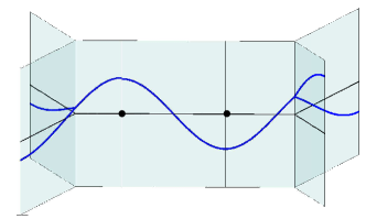
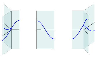
Figure 2.1. On the left, a graph of an eigenfunction $f$ over a tree graph $\Gamma_{\vec{l}}$, $\left\{\left(x,y,f\left(x,y\right)\right)\,\,:\,\,\left(x,y\right)\in\Gamma_{\vec{l}}\right\}$. $f$ has two marked Neumann points. On the right, the Neumann partition of $\Gamma_{\vec{l}}$ according to $f$.

Remark 2.25.

A nodal\Neumann domain is a connected metric graph on its own. We will consider Neumann domains as standard quantum graphs.

3. Neumann count bounds

In this short section we prove uniform bounds on the Neumann count, similarly to the bounds obtained for the nodal count. The nodal count bounds are given by:

Theorem 3.1.

[73, 27, 15] Let $\Gamma_{\vec{l}}$ be a standard graph and assume that $f_{n}$ is generic, then its nodal count is bounded by

(3.1) $$0\leq\phi\left(f_{n}\right)-n\leq\beta,$$

where $\beta$ is the first Betti number of $\Gamma$ (2.1).

Definition 3.2.

Let $\Gamma_{\vec{l}}$ be a standard graph and assume that $f_{n}$ is generic. The nodal surplus of $f_{n}$ is define by

(3.2) $$\sigma\left(f_{n}\right):=\phi\left(f_{n}\right)-n,$$

and the nodal surplus sequence $\sigma:\mathcal{G}\rightarrow\left\{0,1,...\beta\right\}$ is given by $\sigma\left(n\right):=\sigma\left(f_{n}\right)$. We define the Neumann surplus of $f_{n}$ in the same way, denoting

(3.3) $$\omega\left(f_{n}\right):=\mu\left(f_{n}\right)-n,$$

with the Neumann surplus sequence $\omega:\mathcal{G}\rightarrow\mathbb{Z}$ given by $\omega\left(n\right):=\omega\left(f_{n}\right)$.

Remark 3.3.

We call it Neumann surplus as an analog of the nodal surplus, however one should be aware that we do not suggest it is a non-negative quantity (unlike the nodal surplus). We do allow a ’negative surplus’ . For example, the Neumann surplus is always negative for trees, as follows from the next theorem.

Theorem 3.4.

[6] Let $\Gamma_{\vec{l}}$ be a standard graph whose first Betti number is $\beta$ and whose boundary size is $\left|\partial\Gamma\right|$. Then the Neumann surplus sequence is uniformly bounded by

(3.4) $$\forall n\in\mathcal{G}\,\,\,\,\,\,\,\,1-\beta-\left|\partial\Gamma\right|\leq\omega(n)\leq 2\beta-1.$$

This theorem follows from the next lemma that will be useful for other proofs as well.

Lemma 3.5.

Let $f$ be a real generic eigenfunction of $\Gamma_{\vec{l}}$ with eigenvalue $k>0$, and let $\phi\left(f\right)$ and $\mu\left(f\right)$ be its nodal and Neumann counts. Then the difference $\phi\left(f\right)-\mu\left(f\right)$ is given by:

(3.5) $$\phi\left(f\right)-\mu\left(f\right) =\frac{\left|\partial\Gamma\right|}{2}-\frac{1}{2}\sum_{v\in\mathcal{V}_{in}}\sum_{e\in\mathcal{E}_{v}}\mathrm{sign}\left(f\left(v\right)\partial_{e}f\left(v\right)\right).$$

Proof.

Let $e$ be an edge of length $l_{e}$ and vertices $v,u$ (not necessarily distinct). Let $\phi\left(f|_{e}\right)$ be the number of nodal point on $e$ and similarly $\mu\left(f|_{e}\right)$ for Neumann points. Consider the amplitude-phase pair $A_{e},\varphi_{e}$ (see Definition 2.16) such that $f|_{e}\left(x_{e}\right)=A_{e}\cos\left(kx_{e}-\varphi\right)$ and $f|_{e}^{\prime}\left(x_{e}\right)=-kA_{e}\sin\left(kx_{e}-\varphi\right)$. As $f$ is generic, then $A_{e}\neq 0$ and so the nodal points and Neumann points on $e$ interlace and their union is the finite set $\left\{x_{e}\in\left(0,l_{e}\right)\,\,:\,\,kx_{e}-\varphi\in\frac{\pi}{2}\mathbb{Z}\right\}$. Let $N=\phi\left(f|_{e}\right)+\mu\left(f|_{e}\right)$ and number the points

$$\left\{x_{j}\right\}_{j=1}^{N}:=\left\{x_{e}\in\left(0,l_{e}\right)\,\,:\,\,kx_{e}-\varphi\in\frac{\pi}{2}\mathbb{Z}\right\},$$

in increasing order according to the distance from $v$. Let $\delta\left(x_{j}\right)=\begin{cases}1&x_{j}\,\,is\,\,nodal\\ -1&x_{j}\,\,is\,\,Neumann\end{cases}$ so that $\phi\left(f|_{e}\right)-\mu\left(f|_{e}\right)=\sum_{j=1}^{N}\delta\left(x_{j}\right)$. If $N=0$, then $\phi\left(f|_{e}\right)-\mu\left(f|_{e}\right)=0$. If $N=1$, then

$$\phi\left(f|_{e}\right)-\mu\left(f|_{e}\right)=\delta\left(x_{1}\right)=\frac{\delta\left(x_{1}\right)+\delta\left(x_{N}\right)}{2}.$$

If $N>1$, then

$$\phi\left(f|_{e}\right)-\mu\left(f|_{e}\right)=\frac{\delta\left(x_{1}\right)+\delta\left(x_{N}\right)}{2}+\sum_{j=1}^{N-1}\frac{\delta\left(x_{j}\right)+\delta\left(x_{j+1}\right)}{2}=\frac{\delta\left(x_{1}\right)+\delta\left(x_{N}\right)}{2}.$$

Where the last equality follows from the interlacing. We deduce that:

(3.6) $$\phi\left(f|_{e}\right)-\mu\left(f|_{e}\right)=\begin{cases}\frac{\delta\left(x_{1}\right)+\delta\left(x_{N}\right)}{2}&N>0\\ 0&N=0\end{cases}$$ .

Assume that $N>0$. Recall that $f\left(v\right)\neq 0$ as $f$ is generic, and let g$\left(x_{e}\right):=\frac{f\left(v\right)}{k}f|_{e}\left(x_{e}\right)$ so that it is positive and monotone in the interval $x_{e}\in\left(0,x_{1}\right)$. If $x_{1}$ is a nodal point, then $g$ must be decreasing in the interval and if $x_{2}$ is Neumann, then $g$ must be increasing in the interval. Notice that $g$ is monotone and $g^{\prime\prime}\left(0\right)=\frac{f\left(v\right)}{k}f|_{e}^{\prime\prime}\left(0\right)=-k\left(f\left(v\right)\right)^{2}<0$ so $g$ is decreasing unless $g^{\prime}\left(0\right)>0$. Since $g^{\prime}\left(0\right)=f\left(v\right)\partial_{e}f\left(v\right)$, we get

(3.7) $$\delta\left(x_{1}\right)=\begin{cases}1&f\left(v\right)\partial_{e}f\left(v\right)\leq 0\\ -1&f\left(v\right)\partial_{e}f\left(v\right)>0\end{cases}.$$

The same argument relates $\delta\left(x_{N}\right)$ to $f\left(u\right)\partial_{e}f\left(u\right)$ such that

(3.8) $$\frac{\delta\left(x_{1}\right)+\delta\left(x_{N}\right)}{2}=\begin{cases}\frac{1}{2}&f\left(v\right)\partial_{e}f\left(v\right)\leq 0\\ -\frac{1}{2}&f\left(v\right)\partial_{e}f\left(v\right)>0\end{cases}+\begin{cases}\frac{1}{2}&f\left(u\right)\partial_{e}f\left(u\right)\leq 0\\ -\frac{1}{2}&f\left(u\right)\partial_{e}f\left(u\right)>0\end{cases}.$$

If $N=0$, then $g$ is monotone on $\left(0,l_{e}\right)$, $g^{\prime}\left(0\right)=f\left(v\right)\partial_{e}f\left(v\right)$ and $-g^{\prime}\left(l_{e}\right)=f\left(u\right)\partial_{e}f\left(u\right)$. At least one vertex of $e$ must be interior vertex, with out loss of generality assume that $\mathrm{deg}(u)\neq 1$. Then $f$ being generic implies that $g^{\prime}\left(l_{e}\right)\neq 0$. Since $g^{\prime\prime}\left(0\right)<0$ and $g^{\prime}$ does not vanish on $\left(0,l_{e}\right]$, then either $g^{\prime}\left(0\right)=0$ and $g^{\prime}\left(l_{e}\right)<0$ or $g^{\prime}\left(0\right)$ is of the same sign as $g^{\prime}\left(l_{e}\right)$. Namely, the RHS of (3.8) vanish. The genericity assumption gives $g^{\prime}\left(0\right)=0\iff\mathrm{deg}(v)=1$, and so the latter argument together with (3.6) and (3.8) would give, both for $N\neq 0$ and $N=0$, that

(3.9) $$\phi\left(f|_{e}\right)-\mu\left(f|_{e}\right)=\begin{cases}-\frac{\mathrm{sign}\left(f\left(v\right)\partial_{e}f\left(v\right)\right)+\mathrm{sign}\left(f\left(u\right)\partial_{e}f\left(u\right)\right)}{2}&\mathrm{deg}(v),\mathrm{deg}(u)\neq 1\\ \frac{1-\mathrm{sign}\left(f\left(u\right)\partial_{e}f\left(u\right)\right)}{2}&\mathrm{deg}(v)=1\end{cases}.$$

Summing up over all edges, and rearranging the sum to vertices and adjacent edges, gives

$$\phi\left(f\right)-\mu\left(f\right) =\frac{1}{2}\sum_{v\in\mathcal{V}}\sum_{e\in\mathcal{E}_{v}}\begin{cases}1&\mathrm{deg}(v)=1\\ -\mathrm{sign}\left(f\left(v\right)\partial_{e}f\left(v\right)\right)&\mathrm{deg}(v)\neq 1\end{cases}$$

$$= \frac{\left|\partial\Gamma\right|}{2}-\frac{1}{2}\sum_{v\in\mathcal{V}_{in}}\sum_{e\in\mathcal{E}_{v}}\mathrm{sign}\left(f\left(v\right)\partial_{e}f\left(v\right)\right).$$

∎

The proof of Theorem 3.4 is almost immediate:

Proof.

Let $f_{n}$ be a real generic eigenfunction. By definition $\phi(n)-\mu(n)=\sigma(n)-\omega(n)$ and according to Lemma 3.5,

$$\left|\sigma(n)-\omega(n)-\frac{\left|\partial\Gamma\right|}{2}\right| \leq\left|\frac{1}{2}\sum_{v\in\mathcal{V}_{in}}\sum_{e\in\mathcal{E}_{v}}\mathrm{sign}\left(f_{n}\left(v\right)\partial_{e}f_{n}\left(v\right)\right)\right|$$

$$\leq \frac{1}{2}\sum_{v\in\mathcal{V}_{in}}\left|\sum_{e\in\mathcal{E}_{v}}\mathrm{sign}\left(f_{n}\left(v\right)\partial_{e}f_{n}\left(v\right)\right)\right|.$$

Given an interior vertex $v\in\mathcal{V}_{in}$, every $f_{n}\left(v\right)\partial_{e}f_{n}\left(v\right)$ is real and non zero since $f$ is real and generic. The Neumann condition on $v$ implies that $\sum_{e\in\mathcal{E}_{v}}f_{n}\left(v\right)\partial_{e}f_{n}\left(v\right)=0$, so at least one summand is positive and one is negative and so

$$\left|\sum_{e\in\mathcal{E}_{v}}\mathrm{sign}\left(f_{n}\left(v\right)\partial_{e}f_{n}\left(v\right)\right)\right|\leq\mathrm{deg}(v)-2,$$

which means that

$$\left|\sigma(n)-\omega(n)-\frac{\left|\partial\Gamma\right|}{2}\right| \leq\frac{1}{2}\sum_{v\in\mathcal{V}_{in}}\left(\mathrm{deg}(v)-2\right)$$

$$= \frac{1}{2}\sum_{v\in\mathcal{V}}\left(\mathrm{deg}(v)-2\right)-\frac{1}{2}\sum_{v\in\partial\Gamma}\left(-1\right)$$

$$= E-V+\frac{1}{2}\left|\partial\Gamma\right|=\beta-1+\frac{1}{2}\left|\partial\Gamma\right|.$$

It follows that

(3.10) $$1-\beta\leq\sigma(n)-\omega(n)\leq\beta-1+\left|\partial\Gamma\right|.$$

Substituting the nodal surplus bounds, $0\leq\sigma(n)\leq\beta$, gives

$$1-\beta-\left|\partial\Gamma\right|\leq\omega(n)=\sigma(n)-\left(\sigma(n)-\omega(n)\right)\leq\beta+\beta-1=2\beta-1.$$

∎

In [6] we provide examples of graphs for which the sequence $\sigma\left(n\right)-\omega\left(n\right)$ achieves both its upper an lower bounds of (3.10). Unlike the difference $\sigma\left(n\right)-\omega\left(n\right)$, we conjecture in [6] that the Neumann surplus bounds in the case of $\beta\geq 2$ can be improved:

Conjecture 3.6.

[6] The Neumann surplus sequence of a standard graph $\Gamma_{\vec{l}}$ with first Betti number $\beta\geq 2$ is bounded by

$$-1-\left|\partial\Gamma\right|\leq\omega\left(n\right)\leq\beta+1.$$

Remark 3.7.

It is shown in [6] that both $\sigma\left(n\right)$ and $\sigma\left(n\right)-\omega\left(n\right)$ can achieve their upper and lower bounds. Therefore, if the conjecture is true, then the nodal surplus sequence and the Neumann surplus sequence are not independent, in terms of the statistics developed in Section 6.

4. The secular manifold

4.1. Introduction to the secular manifold

The secular manifold, that we will define and discuss in the following section, was first introduced in the work of Barra and Gaspard in [23] in which they use ergodic arguments to calculate the level spacing statistics, by means of averages on the secular manifold. The secular manifold appeared to be useful even beyond spectral statistics. For example, it was used by Colin de Verdière in [57] to prove that there is no quantum unique ergodicity in quantum graph and to describe the possible semiclassical limiting measures. It is also used by Band in [12], proving an inverse problem of showing that the nodal count $\phi\left(n\right)=n$ implies the graph is a tree. In a recent work of Kurasov and Sarnak [89], they analyze the secular manifold from an algebraic point of view. In this work, they classified the spectrum of certain quantum graphs as crystalline measures that contain only finite arithmetic progression with a uniform bound on the lengths of these progressions.

4.2. Abstract definition of the secular manifold

Given $k>0$ we denote the $k^{2}$ eigenspace of $\Gamma_{\vec{l}}$ by $Eig\left(\Gamma_{\vec{l}},k^{2}\right)$. That is $Eig\left(\Gamma_{\vec{l}},k^{2}\right)=\ker\left(\Delta-k^{2}\right)$ restricted to the domain of Neumann vertex conditions. A scaling of the graph by a factor of $t>0$, $\Gamma_{\vec{l}}\mapsto\Gamma_{t\vec{l}}$, induces a bijection $f\left(x\right)\mapsto f\left(\frac{x}{t}\right)$ between $H^{2}\left(\Gamma_{\vec{l}}\right)$ and $H^{2}\left(\Gamma_{t\vec{l}}\right)$. It is not hard to deduce that it preserves the values of $f$ on vertices and scale the derivatives by a factor of $\frac{1}{t}$. In particular, it preserve the Neumann vertex conditions. If $f\in Eig\left(\Gamma_{\vec{l}},k^{2}\right)$ for $k>0$, then $f\left(\frac{x}{k}\right)$ on $\Gamma_{k\vec{l}}$ satisfy Neumann vertex conditions and $-\frac{d^{2}}{d^{2}x_{e}}f|_{e}\left(\frac{x_{e}}{k}\right)=\frac{1}{k^{2}}k^{2}f|_{e}\left(\frac{x_{e}}{k}\right)=f|_{e}\left(\frac{x_{e}}{k}\right)$ on every edge and so $f\left(\frac{x}{k}\right)\in Eig\left(\Gamma_{k\vec{l}},1\right)$. A simple check shows that all amplitudes in Definition 2.16 are preserved under such scaling, and so for any $k>0$ and $\vec{l}\in\left(\mathbb{R}_{+}\right)^{\mathcal{E}}$, $Eig\left(\Gamma_{\vec{l}},k^{2}\right)$ and $Eig\left(\Gamma_{k\vec{l}},1\right)$ are isomorphic by a map which preserves all amplitudes.

Consider $Eig\left(\Gamma_{\vec{l}},1\right)$ and let $\vec{l}$ range over $\left(\mathbb{R}_{+}\right)^{\mathcal{E}}$. The restrictions of any $f\in Eig\left(\Gamma_{\vec{l}},1\right)$ to edges are $2\pi$ periodic (see Definition 2.16), and so $f$ can be extended uniquely to $\Gamma_{l+2\pi\boldsymbol{n}}$ for any $\boldsymbol{n}\in\mathbb{N}^{\mathcal{E}}$. This extension is a linear bijection between $Eig\left(\Gamma_{\vec{l}},1\right)$ and $Eig\left(\Gamma_{\vec{l}+2\pi\boldsymbol{n}},1\right)$ which preserves all amplitudes. In fact this is true for all $\boldsymbol{n}\in\mathbb{Z}^{\mathcal{E}}$ such that $\vec{l}+2\pi\boldsymbol{n}\in\mathbb{R}_{+}^{\mathcal{E}}$. We can conclude that for any $\vec{l}\in\left(\mathbb{R}_{+}\right)^{E},k>0$ and $\boldsymbol{n}\in\mathbb{Z}^{\mathcal{E}}$ such that $k\vec{l}+2\pi\boldsymbol{n}\in\mathbb{R}_{+}^{\mathcal{E}}$:

(4.1) $$Eig\left(\Gamma_{\vec{l}},k^{2}\right)\underset{{}_{Scaling\,by\,k}}{\underbrace{\cong}}Eig\left(\Gamma_{k\vec{l}},1\right)\underset{{}_{extending\,by\,\boldsymbol{n}}}{\underbrace{\cong}}Eig\left(\Gamma_{k\vec{l}+2\pi\boldsymbol{n}},1\right),$$

with an isomorphism that preserves all amplitudes from Definition 2.16.

Remark 4.1.

One may ask what happens for $k=0$, as we cannot scale the graph by $0$, but we would expect an isomorphism between $Eig\left(\Gamma_{\vec{l}},0\right)$ and $Eig\left(\Gamma_{2\pi\boldsymbol{n}},1\right)$ for any $\boldsymbol{n}\in\mathbb{N}^{\mathcal{E}}$. It appears that this isomorphism holds only for tree graphs. In the following subsection we will show that $\dim Eig\left(\Gamma_{2\pi\boldsymbol{n}},1\right)=\beta+1$, where $\beta$ is the first Betti number of $\Gamma_{\vec{l}}$. As we already mentioned that $0$ is always a simple eigenvalue (since $\Gamma$ is connected), then $Eig\left(\Gamma_{\vec{l}},0\right)\not\cong Eig\left(\Gamma_{2\pi\boldsymbol{n}},1\right)$ if $\beta>0$. In the $\beta=0$ case, namely a tree, the mapping of $f\equiv C$ to $\tilde{f}\in Eig\left(\Gamma_{2\pi\boldsymbol{n}},1\right)$ given by $\tilde{f}|_{e}\left(x_{e}\right):=C\cos\left(x_{e}\right)$, is a bijection between $Eig\left(\Gamma_{\vec{l}},0\right)$ and $Eig\left(\Gamma_{2\pi\boldsymbol{n}},1\right)$ that preserve the trace of the functions.

It is clear from (4.1) that given any $\vec{l}$ and any $k^{2}>0$ eigenvalue of $\Gamma_{\vec{l}}$, if we denote $\tilde{l}\in\left(0,2\pi\right]^{\mathcal{E}}$ such that $\tilde{l}=k\vec{l}\,\,\,mod\,2\pi$ then, $Eig\left(\Gamma_{\vec{l}},k^{2}\right)\cong Eig\left(\Gamma_{\tilde{l}},1\right)$ by (4.1). The secular manifold, to be defined next, is the set of all such $\tilde{l}$ for every possible pair of $\vec{l}$ and $k^{2}>0$.

Definition 4.2.

We denote the flat torus $\mathbb{T}^{n}:=\left(\mathbb{R}/2\pi\mathbb{Z}\right)^{n}$ for every $n\in\mathbb{N}$, and define the characteristic torus of a graph by $\mathbb{T}^{\mathcal{E}}$. We use the notation $\left\{*\right\}:\mathbb{R}^{\mathcal{E}}\rightarrow\mathbb{T}^{\mathcal{E}}$ to denote $\left\{\vec{x}\right\}=\vec{x}\,\,\,mod\,2\pi$.

Definition 4.3.

Given a discrete graph $\Gamma$, for every point $\vec{\kappa}\in\mathbb{T}^{\mathcal{E}}$ we associate a standard graph denoted by $\Gamma_{\vec{\kappa}}$, whose edge lengths are $\vec{l}\in\left(0,2\pi\right]^{\mathcal{E}}$ such that $\left\{\vec{l}\right\}=\vec{\kappa}$. The secular manifold of $\Gamma$ is defined as follows:

(4.2) $$\Sigma:=\left\{\vec{\kappa}\in\mathbb{T}^{E}\,\,:\,\,\dim Eig\left(\Gamma_{\vec{\kappa}},1\right)\geq 1\right\}.$$

We partition $\Sigma$ into “singular” and “regular” parts which are define as follows:

(4.3) $$\Sigma^{reg} :=\left\{\vec{\kappa}\in\Sigma\,\,:\,\,\dim Eig\left(\Gamma_{\vec{\kappa}},1\right)=1\right\},$$

(4.4) $$\Sigma^{sing} :=\left\{\vec{\kappa}\in\Sigma\,\,:\,\,\dim Eig\left(\Gamma_{\vec{\kappa}},1\right)>1\right\}.$$

It is now clear from (4.1) that:

Lemma 4.4.

Let $\Gamma_{\vec{l}}$ be a standard graph, let $k^{2}>0$ and let $\vec{\kappa}=\left\{k\vec{l}\right\}$. Then $k^{2}$ is an eigenvalue of $\Gamma_{\vec{l}}$ if and only if $\vec{\kappa}\in\Sigma$ and it is a simple eigenvalue if and only if $\vec{\kappa}\in\Sigma^{reg}$.

The terms “regular” and “singular” in Definition 4.3 refer to the structure of the secular manifold as presented in the following proposition.

Definition 4.5.

[113] A real analytic manifold is a smooth manifold whose transition maps are real analytic. Given a real analytic function $f:\mathbb{R}^{n}\rightarrow\mathbb{R}^{m}$, its zero set $Z_{f}$ is called a real analytic variety. A point $x\in Z_{f}$ is called regular if it has a neighborhood of $Z_{f}$ which is a manifold, and is called singular if it is not regular. The regular part of $Z_{f}$ which we denote by $Z_{f}^{reg}$ is the union of regular points. The dimension of $Z_{f}$ is the maximal dimension of neighborhoods of regular points.

Proposition 4.6.

Given a graph $\Gamma$ with $E$ edges, its secular manifold $\Sigma$ is a real analytic variety of dimension $E-1$. The set $\Sigma^{reg}$ that was defined in (4.3) is the set of regular points of $\Sigma$, and it is a real analytic manifold of dimension $E-1$. The set $\Sigma^{sing}$ that was defined in (4.4) is the set of singular points of $\Sigma$, and it is a real analytic variety of dimension strictly smaller than $E-1$ (positive co-dimension in $\Sigma$).

A proof for this proposition will be given in Subsection 4.4, but we will state here two usefull lemmas regarding real analytic varieties that will be used in the proof of Proposition 4.6 as well as in other proofs.

Lemma 4.7.

[113]  If $Z_{f}$ is a real analytic variety of dimension $n$, then it has the following stratification $Z_{f}=\cup_{j=0}^{n}S_{j}$ where every $S_{j}$, which is called a strata, is a $j$-dimensional real analytic manifold (possibly empty).

Lemma 4.8.

Let $M$ be a connected real analytic manifold and let $h$ be a real analytic function on $M$ which is not the zero function. Then the zero set

(4.5) $$Z_{h}:= \left\{\vec{x}\in M\,\,:\,\,h\left(\vec{x}\right)=0\right\},$$

is a real analytic variety of positive co-dimension in $M$.

Proof.

Clearly, if $M$ is a zero set of a real analytic function $f$, then $Z_{h}$ is the zero set of the real analytic function $\left(f,h\right)$ and is therefore an analytic variety. Let $\left\{O_{n},\varphi_{n}\right\}_{n\in\mathbb{N}}$ be the real analytic atlas of $M$, with $\left\{U_{n}\right\}_{n\in\mathbb{N}}$ open subsets of $\mathbb{R}^{d}$ (where $d=\dim\left(M\right)$), each $U_{n}$ diffeomorphic to $O_{n}$ by $U_{n}=\varphi_{n}\left(O_{n}\right)$. Let $h_{n}:=h\circ\varphi_{n}^{-1}$ so that by definition $h_{n}:U_{n}\rightarrow\mathbb{R}$ is real analytic. By proposition 3 in [96] the zero set of $h_{n}$ is of positive co-dimension in $U_{n}$ and therefore its preimage by $\varphi_{n}$, $Z_{h}\cap O_{n}$ has positive co-dimension in $M$. Therefore $Z_{h}$ is a countable union of sets of positive co-dimension and as such has positive co-dimension. ∎

4.3. Canonical eigenfunctions

In the context of quantum mechanics and spectral theory it is standard to consider eigenfunctions which are $L^{2}$ normalized. However, in our context a different normalization would be more convenient.

Definition 4.9.

Given an eigenfunction $f$ with amplitudes vector $\boldsymbol{a}\in\mathbb{C}^{\vec{\mathcal{E}}}$ as defined in Definition 2.16, we say that $f$ is normalized if $\left\|\boldsymbol{a}\right\|=1$ (Euclidean norm).

For a regular point $\vec{\kappa}\in\Sigma^{reg}$, where $\dim Eig\left(\Gamma_{\vec{\kappa}},1\right)=1$, we define a canonical choice (up to sign) of eigenfunction $f_{\vec{\kappa}}\in Eig\left(\Gamma_{\vec{\kappa}},1\right)$.

Definition 4.10.

Let $\vec{\kappa}\in\Sigma^{reg}$, we define its canonical eigenfunction as the unique (up to a sign) normalized real eigenfunction $f_{\vec{\kappa}}\in Eig\left(\Gamma_{\vec{\kappa}},1\right)$.

Lemma 4.11.

Let $\Gamma_{\vec{l}}$ be a standard graph, let $k^{2}>0$ be a simple eigenvalue of $\Gamma_{\vec{l}}$ with a normalized real eigenfunction $f$ and let $\vec{\kappa}=\left\{k\vec{l}\right\}\in\Sigma^{reg}$ with canonical eigenfunction $f_{\vec{\kappa}}$. Then $f$ and $f_{\vec{\kappa}}$ share the same amplitudes vector and so their traces are related as follows:

(4.6) $$\forall v\in\mathcal{V},\,\,\forall e\in\mathcal{E}_{v}\,\,\,\,\,\,f_{\vec{\kappa}}\left(v\right)=f\left(v\right)\,\,\,\,\,and\,\,\,\,\partial_{e}f_{\vec{\kappa}}\left(v\right)=\frac{\partial_{e}f\left(v\right)}{k}.$$

Where the equalities are up to a global sign.

Proof.

The bijection between $Eig\left(\Gamma_{\vec{l}},k^{2}\right)$ and $Eig\left(\Gamma_{\vec{\kappa}},1\right)$ is given as a composition of two maps, scaling by $k$ and extensions of the edges by integer multiples of $2\pi$. Let $\tilde{f}\in Eig\left(\Gamma_{k\vec{l}},1\right)$ given by the scaling bijection, namely $\tilde{f}|_{e}\left(x_{e}\right)=f|_{e}\left(\frac{x_{e}}{k}\right)$ $\forall e\in\mathcal{E},\forall x_{e}\in\left[0,kl_{e}\right]$. It is not hard to deduce that $f\left(v\right)=\tilde{f}\left(v\right)$ and $\partial_{e}f\left(v\right)=k\partial_{e}\tilde{f}\left(v\right)$ for every $v\in\mathcal{V},e\in\mathcal{E}_{v}$. Therefore, according to the relations between the trace and amplitudes in Lemma 2.16 (1), $\tilde{f}$ and $f$ share the same amplitudes and therefore $\tilde{f}$ is also real with normalized amplitudes vector. It is not hard to deduce that the second bijection, the extension by integer multiples of $2\pi$, does not change the trace and the amplitudes vector, and therefore $\tilde{f}$ is mapped to a real eigenfunction in $Eig\left(\Gamma_{\vec{\kappa}},1\right)$ with normalized amplitudes vector, namely $\pm f_{\vec{\kappa}}$. This proves the lemma. ∎

4.4. Wave scattering and explicit construction of the secular manifold.

The scattering approach was first applied to quantum graphs by Von Below [122] and later on by Kottos and Smilansky in [84, 83]. In this subsection we review this procedure and use it to construct the secular manifold. For more information on the scattering approach we refer the reader to [33, 71].

Let $f$ be a real eigenfunction of a standard graph $\Gamma_{\vec{l}}$ with eigenvalue $k^{2}>0$, and denote its amplitudes vector by $\boldsymbol{a}\in\mathbb{C}^{\vec{\mathcal{E}}}$ (see Definition 2.16 (1)). The vertex conditions on a vertex $v\in\mathcal{V}$ provides $\mathrm{deg}(v)$ linear equations on $\mathrm{trace}\left(f\right)$:

$$f|_{e}\left(v\right) =f|_{e^{\prime}}\left(v\right)\,\,\,\forall e,e^{\prime}\in\mathcal{E}_{v},$$

$$\sum_{e\in\mathcal{E}_{v}}\partial_{e}f\left(v\right) =0,$$

which can be written, using Definition 2.16, (1), as $\mathrm{deg}(v)$ linear equations on $a$ with coefficients that are linear in $\left\{e^{ikl_{e}}\right\}_{e\in\mathcal{E}}$. Over all, it is a system of $\sum_{v\in\mathcal{V}}\mathrm{deg}(v)=2E=\left|\vec{\mathcal{E}}\right|$ linear equations on $a$ that can be rearranged as such (see [71, 33] for detailed explanation):

(4.7) $$\left(1-U_{k\vec{l}}\right)a=0,$$

where $U_{k\vec{l}}$ is unitary matrix from $\mathbb{C}^{\vec{\mathcal{E}}}$ to itself, called the unitary evolution matrix, whose entries are linear functions of $\left\{e^{ikl_{e}}\right\}_{e\in\mathcal{E}}$. We define $U_{\vec{\kappa}}$ accordingly as function of $\vec{\kappa}\in\mathbb{T}^{\mathcal{E}}$ such that $U_{k\vec{l}}=U_{\vec{\kappa}}$ for $\vec{\kappa}=\left\{k\vec{l}\right\}$. Notice that the mapping $a\mapsto f$ given by the restrictions $f|_{e}\left(x_{e}\right)=a_{e}e^{-ikl_{e}}e^{ikx}+a_{\hat{e}}e^{-ikx}$ is a linear bijection (according to Definition 2.16 (1) ) between $\mathbb{C}^{\vec{\mathcal{E}}}$ and functions that satisfy $f^{\prime\prime}=-k^{2}f$ edgewise. As the vertex conditions of $f$ in terms of $\boldsymbol{a}$ are given in (4.7), then

(4.8) $$f\in Eig\left(\Gamma_{\vec{\kappa}},1\right) \iff\boldsymbol{a}\in\ker\left(1-U_{k\vec{l}}\right).$$

We may deduce the following lemma:

Lemma 4.12.

The mapping $\boldsymbol{a}\mapsto f$ given by Definition 2.16 (1) is a linear bijection between $\ker\left(1-U_{k\vec{l}}\right)$ and $Eig\left(\Gamma_{\vec{l}},k^{2}\right)$ for $k>0$. In particular, $Eig\left(\Gamma_{\vec{\kappa}},1\right)\cong\ker\left(1-U_{\vec{\kappa}}\right)$ for any $\vec{\kappa}\in\mathbb{T}^{\mathcal{E}}$ and $\Sigma$ is the zero set of $\det\left(1-U_{\vec{\kappa}}\right)$. This allows to express (4.3) and (4.4) as

(4.9) $$\Sigma^{reg} :=\left\{\vec{\kappa}\in\Sigma\,\,:\,\,\dim\ker\left(1-U_{\vec{\kappa}}\right)=1\right\},$$

(4.10) $$\Sigma^{sing} :=\left\{\vec{\kappa}\in\Sigma\,\,:\,\,\dim\ker\left(1-U_{\vec{\kappa}}\right)>1\right\}.$$

The structure of $U_{\vec{\kappa}}$ and its $\vec{\kappa}$ dependence are given by a product of two unitary matrices

(4.11) $$U_{\vec{\kappa}}=e^{i\vec{\kappa}}S.$$

This is a decomposition of $U$ to a $\vec{\kappa}$ dependent matrix $e^{i\vec{\kappa}}$ and a fixed real orthogonal matrix $S$ which is called the bond-scattering matrix. The matrix $e^{i\vec{\kappa}}$ is a unitary diagonal matrix with diagonal entries

(4.12) $$\forall e\in\mathcal{E}\,\,\left(e^{i\vec{\kappa}}\right)_{e,e}=\left(e^{i\vec{\kappa}}\right)_{\hat{e},\hat{e}}=e^{i\kappa_{e}}.$$

Given two directed edges $e$ and $e^{\prime}$ that are connected by a vertex $v$, we write $e\xrightarrow[v]{}e^{\prime}$ if $e$ is directed into $v$ and $e^{\prime}$ is directed out of $v$. The matrix $S$ satisfies $\left(S\right)_{e,e^{\prime}}\neq 0$ if and only if $e^{\prime}\xrightarrow[v]{}e$. In such case, if $e\xrightarrow[v]{}e^{\prime}$, then

(4.13) $$\left(S\right)_{e,e^{\prime}}=\begin{cases}\frac{2}{\mathrm{deg}(v)}-1&if\,e^{\prime}=\hat{e}\\ \frac{2}{\mathrm{deg}(v)}&otherwise\end{cases},$$

where $\hat{e}$ denotes the opposite direction of $e$. If we introduce the reflection $J$, a permutation matrix defined by $J\left(e\right)=\hat{e}$ for every directed edge, then it is not hard to deduce that $JS$ is block diagonal with blocks that we denote by $\left(JS\right)_{v}$ corresponding to edges that are directed into the vertex $v$. Every off-diagonal entry of the block $\left(JS\right)_{v}$ is equal to $\frac{2}{\mathrm{deg}(v)}$ and every diagonal entry is equal to $\frac{2}{\mathrm{deg}(v)}-1$. Notices that $JS=2P-1$ where $P$ is the $\mathrm{deg}(v)\times\mathrm{deg}(v)$ matrix all of whose entries are $\frac{1}{\mathrm{deg}(v)}$. It is a simple check to see that $P$ is a rank one orthogonal projection and therefore $\det\left(JS\right)_{v}=\det\left(2P-1\right)_{v}=\left(-1\right)^{\mathrm{deg}(v)-1}$. It is easy to show that in the basis of $\left(e_{1},\hat{e}_{1},e_{2},\hat{e}_{2}...\right)$, $J$ is block diagonal with blocks $\begin{pmatrix}0&1\\ 1&0\end{pmatrix}$ and so $\det\left(J\right)=\left(-1\right)^{E}$. Therefore, $\det\left(S\right)=\left(-1\right)^{\sum_{v}\mathrm{deg}(v)-V+E}=\left(-1\right)^{\beta-1}$, using $\sum_{v}\mathrm{deg}(v)=2E$ and $\beta=E-V+1$. This gives

(4.14) $$\det\left(U_{\vec{\kappa}}\right)=\left(-1\right)^{\beta-1}\det\left(e^{i\vec{\kappa}}\right)=\left(-1\right)^{\beta-1}e^{i\sum_{e\in\mathcal{E}}2\kappa_{e}}.$$

Remark 4.13.

This construction can be done to arbitrary vertex conditions (by changing $S$ accordingly) and not only Neumann vertex conditions. But if the vertex conditions are not preserved under the scaling $f\left(x\right)\mapsto f\left(\frac{x}{k}\right)$ then the matrix $S$ depends on the eigenvalue $k^{2}$. In such case $\ker\left(1-U_{k\vec{l}}\right)\cong Eig\left(\Gamma_{k\vec{l}},1\right)$ but these are not isomorphic to $Eig\left(\Gamma_{\vec{l}},k^{2}\right)$ in general, and the analysis on the secular manifold can not be proceeded. A possible solution for general vertex conditions is to consider an asymptotic $k$ dependent scattering matrix [33, 71, 109].

As stated in Lemma 4.12, $\Sigma$ is the zero set of $\det\left(1-U_{\vec{\kappa}}\right)$. As $\det\left(1-U_{\vec{\kappa}}\right)$ is a complex function we define a real function that vanish whenever $\det\left(1-U_{\vec{\kappa}}\right)$ does.

Definition 4.14.

We define the secular function on $\mathbb{T}^{\mathcal{E}}$ by

(4.15) $$F\left(\vec{\kappa}\right):= \det\left(U_{\vec{\kappa}}\right)^{-\frac{1}{2}}\det\left(1-U_{\vec{\kappa}}\right),$$

where we consider the square-root branch $\det\left(U_{\vec{\kappa}}\right)^{-\frac{1}{2}}=i^{\left(\beta-1\right)}e^{-i\sum_{e\in\mathcal{E}}\kappa_{e}}$.

Our “implicit” definition of the secular manifold and its partition to regular and singular in Definition 4.3 is different than its “explicit” definition as the zero set of the secular function, as was defined in prior works such as [23, 40, 57] for example. The following lemma justify the equivalence of these definitions:

Lemma 4.15.

The secular function $F$ is a real (multi-variable) trigonometric polynomial. The secular manifold $\Sigma$ is the zero set of $F$, and its singular part is the set on which $\nabla F=0$. That is,

(4.16) $$\Sigma =\left\{\vec{\kappa}\in\mathbb{T}^{\mathcal{E}}\,\,:\,\,F\left(\vec{\kappa}\right)=0\right\}$$

(4.17) $$\Sigma^{reg} =\left\{\vec{\kappa}\in\mathbb{T}^{\mathcal{E}}\,\,:\,\,F\left(\vec{\kappa}\right)=0\,\,\text{and}\,\,\nabla F\left(\vec{\kappa}\right)\neq 0\right\}$$

(4.18) $$\Sigma^{sing} =\left\{\vec{\kappa}\in\mathbb{T}^{\mathcal{E}}\,\,:\,\,F\left(\vec{\kappa}\right)=0\,\,\text{and}\,\,\nabla F\left(\vec{\kappa}\right)=0\right\}.$$

Remark 4.16.

In [57] the secular manifold is called the ‘determinant manifold’. Both the names follows from the description of $\Sigma$ as the zero set of $F$ and $\det\left(1-U_{\vec{\kappa}}\right)$.

We will prove Lemma 4.15, together with the next lemma that relates the gradient of $F$ at a regular point $\vec{\kappa}$ to the canonical eigenfunction $f_{\vec{\kappa}}$ at that point.

Definition 4.17.

Let $\vec{\kappa}\in\Sigma^{reg}$ and let $f_{\vec{\kappa}}$ be the canonical eigenfunction with amplitudes vector $\boldsymbol{a}$. We define its weights vector $m_{\vec{\kappa}}\in\left[0,1\right]^{\mathcal{E}}$ by

(4.19) $$\left(m_{\vec{\kappa}}\right)_{e}=\left|a_{e}\right|^{2}+\left|a_{\hat{e}}\right|^{2}.$$

Equivalently, if $v\in\mathcal{V}$ is connected to $e$, then $\left(m_{\vec{\kappa}}\right)_{e}=\frac{f_{\vec{\kappa}}\left(v\right)^{2}+\partial_{e}f_{\vec{\kappa}}\left(v\right)^{2}}{2}$.

Remark 4.18.

The above weights play a special role in the work of Colin de Verdière [57] on quantum ergodicity fro quantum graphs.

Definition 4.19.

We define an auxiliary function

(4.20) $$p\left(\vec{\kappa}\right):= -i\det\left(U_{\vec{\kappa}}\right)^{-\frac{1}{2}}\mathrm{trace}\left(\mathrm{adj}\left(1-U_{\vec{\kappa}}\right)\right),$$

where $\det\left(U_{\vec{\kappa}}\right)^{-\frac{1}{2}}=i^{\left(\beta-1\right)}e^{-i\sum_{e\in\mathcal{E}}\kappa_{e}}$ and $\mathrm{adj}\left(1-U_{\vec{\kappa}}\right)$ is the adjugate matrix of $\left(1-U_{\vec{\kappa}}\right)$.

Lemma 4.20.

The auxiliary function $p$ is a trigonometric polynomial, and it is real when restricted to $\Sigma$. The gradient of the secular function $\nabla F$ is proportional to the weights vector $m_{\vec{\kappa}}$ with a factor $p$:

(4.21) $$\forall\vec{\kappa}\in\Sigma^{reg}\,\,\nabla F\left(\vec{\kappa}\right)=p\left(\vec{\kappa}\right)m_{\vec{\kappa}}.$$

In particular, all non-vanishing entries of $\nabla F$ share the same sign. Moreover, the regular and singular parts of $\Sigma$ are characterized by $p$,

(4.22) $$\Sigma^{reg} =\left\{\vec{\kappa}\in\mathbb{T}^{\mathcal{E}}\,\,:\,\,F\left(\vec{\kappa}\right)=0\,\,and\,\,p\left(\vec{\kappa}\right)\neq 0\right\},$$

(4.23) $$\Sigma^{sing} =\left\{\vec{\kappa}\in\mathbb{T}^{\mathcal{E}}\,\,:\,\,F\left(\vec{\kappa}\right)=0\,\,and\,\,p\left(\vec{\kappa}\right)=0\right\},$$

and the normal to $\Sigma^{reg}$ at $\vec{\kappa}$ is given by

(4.24) $$\hat{n}\left(\vec{\kappa}\right)=\frac{m_{\vec{\kappa}}}{\left\|m_{\vec{\kappa}}\right\|}.$$

In order to prove Lemmas 4.15 and 4.20 we need to discuss some properties of the adjugate matrix:

Lemma 4.21.

Let $U$ be a unitary $n$-dimensional matrix with eigenvalues $\left\{e^{i\theta_{j}}\right\}_{j=1}^{n}$ and (orthonormal) eigenvectors $\left\{\boldsymbol{a}_{j}\right\}_{j=1}^{n}$, then

1. The adjugate matrix $\mathrm{adj}\left(1-U\right)$ satisfies

   (4.25) $$\mathrm{adj}\left(1-U\right)=\sum_{j=1}^{n}\Pi_{i\neq j}\left(1-e^{i\theta_{i}}\right)\boldsymbol{a}_{j}\boldsymbol{a}_{j}^{*}.$$

   In particular $\mathrm{adj}\left(1-U\right)=0$ if and only if $\dim\ker\left(1-U\right)\geq 2$.
   

2. Let $\dim\ker\left(1-U\right)=1$ and let $\boldsymbol{a}\in\ker\left(1-U\right)$ be a normalized vector. Let us number the eigenvalues such that $e^{i\theta_{1}}=1$ and $e^{i\theta_{j}}\neq 1$ for $j\geq 2$. Then

   (4.26) $$\mathrm{adj}\left(1-U\right) =\Pi_{j=2}^{n}\left(1-e^{i\theta_{j}}\right)\boldsymbol{a}\boldsymbol{a}^{*},$$

   (4.27) $$\mathrm{trace}\left(\mathrm{adj}\left(1-U\right)\right) =\Pi_{j=2}^{n}\left(1-e^{i\theta_{j}}\right)\neq 0.$$

3. Let $U_{t}$ be a $t\in\mathbb{R}$ dependent family of unitary matrices with a self-adjoint matrix $A$ such that $\frac{d}{dt}U_{t}=iAU_{t}$. Let $t_{0}$ such that $\dim\ker\left(1-U_{t_{0}}\right)=1$ and let $\boldsymbol{a}\in\ker\left(1-U_{t_{0}}\right)$ be a normalized vector . Then

   (4.28) $$\frac{d}{dt}\det\left(1-U_{t}\right)= -i\cdot\mathrm{trace}\left(\mathrm{adj}\left(1-U_{t_{0}}\right)\right)\left\langle\boldsymbol{a},A\boldsymbol{a}\right\rangle.$$

Proof.

If $1-U$ is invertible, then its adjugate matrix satisfies,

(4.29) $$\mathrm{adj}\left(1-U\right)=\det\left(1-U\right)\left(1-U\right)^{-1}.$$

Since $\det\left(1-U\right)=\Pi_{j=1}^{n}\left(1-e^{i\theta_{j}}\right)$ and

$$\left(1-U\right)^{-1}=\sum_{j=1}^{n}\frac{1}{1-e^{i\theta_{j}}}\boldsymbol{a}_{j}\boldsymbol{a}_{j}^{*},$$

then

(4.30) $$\mathrm{adj}\left(1-U\right)=\sum_{j=1}^{n}\frac{1}{1-e^{i\theta_{j}}}\Pi_{i=1}^{n}\left(1-e^{i\theta_{i}}\right)\boldsymbol{a}_{j}\boldsymbol{a}_{j}^{*}=\sum_{j=1}^{n}\Pi_{i\neq j}\left(1-e^{i\theta_{i}}\right)\boldsymbol{a}_{j}\boldsymbol{a}_{j}^{*}.$$

By definition every entry of $\mathrm{adj}\left(1-U\right)$ is a minor of $1-U$ up to a sign, so it is continuous in the entries of $1-U$. As the eigenvalues and eigenvectors are also continuous and invertible matrices are dense within all matrices, then (4.30) may be extended to every matrix with such spectral decomposition, thus proving (4.25). Observe that since $\left\{\boldsymbol{a}_{j}\right\}_{j=1}^{n}$ are orthogonal then a matrix $\sum c_{j}\boldsymbol{a}_{j}\boldsymbol{a}_{j}^{*}$ is equal to zero if and only if every $c_{j}=0$. For the above adjugate matrix, all $\Pi_{i\neq j}\left(1-e^{i\theta_{i}}\right)$ coefficients vanish if and only if there at at least two $e^{i\theta_{j}}$’s that are equal to 1. Namely,

$$\mathrm{adj}\left(1-U\right)=0\iff\dim\ker\left(1-U\right)\geq 2.$$

Clearly, if $e^{i\theta_{1}}=1$ and $e^{i\theta_{j}}\neq 1$ for $j\neq 1$, then the only non-vanishing coefficient is $\Pi_{j=2}^{n}\left(1-e^{i\theta_{j}}\right)$ and so (4.26) follows. As $\boldsymbol{a}$ in (4.26) is normalized, then $\mathrm{trace}\left(\boldsymbol{a}\boldsymbol{a}^{*}\right)=1$ and therefore $\mathrm{trace}\left(\mathrm{adj}\left(1-U\right)\right)=\Pi_{j=2}^{n}\left(1-e^{i\theta_{j}}\right)\neq 0$ proving (4.27). To prove (4.28) we use Jacobi’s identity for the derivative of a matrix and the given relation $\frac{d}{dt}U_{t}=iAU_{t}$:

$$\frac{d}{dt}\left(\det\left(1-U_{t}\right)\right) =\mathrm{trace}\left(\mathrm{adj}\left(1-U_{t}\right)\frac{d}{dt}\left(1-U_{t}\right)\right)$$

$$= -i\cdot\mathrm{trace}\left(\mathrm{adj}\left(1-U_{t}\right)AU_{t}\right).$$

At $t=t_{0}$, using (4.26) and (4.27), we get

$$\frac{d}{dt}\left(\det\left(1-U_{t_{0}}\right)\right) =-i\cdot\mathrm{trace}\left(\mathrm{adj}\left(1-U_{t_{0}}\right)\right)\cdot\mathrm{trace}\left(\boldsymbol{a}\boldsymbol{a}^{*}AU_{t_{0}}\right)$$

$$= -i\cdot\mathrm{trace}\left(\mathrm{adj}\left(1-U_{t_{0}}\right)\right)\cdot\mathrm{trac}e\left(\boldsymbol{a}\boldsymbol{a}^{*}A\right)$$

$$= -i\cdot\mathrm{trace}\left(\mathrm{adj}\left(1-U_{t_{0}}\right)\right)\left\langle\boldsymbol{a},A\boldsymbol{a}\right\rangle.$$

Where in the second step we used $\mathrm{trace}\left(\boldsymbol{a}\boldsymbol{a}^{*}AU_{t_{0}}\right)=\mathrm{trace}\left(U_{t_{0}}\boldsymbol{a}\boldsymbol{a}^{*}A\right)$ and $U_{t_{0}}\boldsymbol{a}=\boldsymbol{a}$ (by the definition of $\boldsymbol{a}$). ∎

We may now prove lemmas 4.15 and 4.20. Although presented separately, it will be convenient to prove both lemmas together:

Proof.

First notice that both $\det\left(1-U_{\vec{\kappa}}\right)$ and $\mathrm{trace}\left(\mathrm{adj}\left(1-U_{\vec{\kappa}}\right)\right)$ are trigonometric polynomials as they are polynomial in the entries of $U_{\vec{\kappa}}$ which are linear in $\left\{e^{i\kappa_{e}}\right\}_{e\in\mathcal{E}}$. Recall that we consider $\det\left(U_{\vec{\kappa}}\right)^{-\frac{1}{2}}=i^{\left(\beta-1\right)}e^{-i\sum_{e\in\mathcal{E}}\kappa_{e}}$ so it is also a trigonometric polynomial, and so both $F$ and $p$ are trigonometric polynomials. Let $\left\{e^{i\theta_{j}}\right\}_{j=1}^{2E}$ be the $\vec{\kappa}$ dependent eigenvalues of $U_{\vec{\kappa}}$ with $\theta_{j}\in\mathbb{R}/2\pi\mathbb{Z}$ for every $j$. Then

$$F\left(\vec{\kappa}\right)=\det\left(U_{\vec{\kappa}}\right)^{-\frac{1}{2}}\det\left(1-U_{\vec{\kappa}}\right)=\pm\Pi_{n=1}^{2E}e^{-i\frac{\theta_{j}}{2}}\left(1-e^{i\theta_{j}}\right)=\pm\left(-2i\right)^{2E}\Pi_{n=1}^{2E}\sin\left(\frac{\theta_{j}}{2}\right),$$

where the $\pm$ ambiguity is due to possible square-root branch choices. The above RHS is real, which proves that $F$ is real and hence a real trigonometric polynomial (and in particular real analytic). Since $\left|p\left(\vec{\kappa}\right)\right|=\left|\mathrm{trace}\left(\mathrm{adj}\left(1-U_{\vec{\kappa}}\right)\right)\right|$ we use Lemma 4.21 to conclude that $p\left(\vec{\kappa}\right)\neq 0$ if $\dim\left(\ker\left(1-U_{\vec{\kappa}}\right)\right)=1$ and that $p\left(\vec{\kappa}\right)=0$ if $\dim\left(\ker\left(1-U_{\vec{\kappa}}\right)\right)\geq 2$ as in such case $\mathrm{adj}\left(1-U_{\vec{\kappa}}\right)=0$. By Lemma 4.12 we may conclude that $p$ is a trigonometric polynomial that vanish on $\Sigma^{sing}$ and is non-zero on $\Sigma^{reg}$. To show that $p$ is real on $\Sigma$, it enough to show it for $\Sigma^{reg}$. If $\vec{\kappa}\in\Sigma^{reg}$, and with out loss of generality $e^{i\theta_{1}}=1$ then according to Lemma 4.21, $\mathrm{trace}\left(\mathrm{adj}\left(1-U_{\vec{\kappa}}\right)\right)=\Pi_{n=2}^{2E}\left(1-e^{i\theta_{j}}\right)\neq 0$, and therefore

$$p\left(\vec{\kappa}\right) =-i\det\left(U_{\vec{\kappa}}\right)^{-\frac{1}{2}}\mathrm{trace}\left(\mathrm{adj}\left(1-U_{\vec{\kappa}}\right)\right)$$

$$= \pm i\Pi_{n=2}^{2E}e^{-i\frac{\theta_{j}}{2}}\left(1-e^{i\theta_{j}}\right)$$

$$= \pm i\left(-2i\right)^{2E-1}\Pi_{n=2}^{2E}\sin\left(\frac{\theta_{j}}{2}\right)\in\mathbb{R}\setminus\left\{0\right\}.$$

It follows that $p$ is real on $\Sigma$. Notice that we cannot deduce from the above that $p$ is a real trigonometric polynomial, but it is clear that $p$ is a real analytic function on $\Sigma$. Both (4.22) and (4.23) follows from

Let $\vec{\kappa}\in\Sigma$ so that $\det\left(U_{\vec{\kappa}}\right)^{\frac{1}{2}}\neq 1$ and $\det\left(1-U_{\vec{\kappa}}\right)=0$, then

(4.31) $$\nabla F\left(\vec{\kappa}\right)=\det\left(U_{\vec{\kappa}}\right)^{\frac{1}{2}}\nabla\det\left(1-U_{\vec{\kappa}}\right).$$

If $\vec{\kappa}\in\Sigma^{sing}$, namely $\dim\ker\left(1-U_{\vec{\kappa}}\right)\geq 2$ then $adj\left(1-U_{\vec{\kappa}}\right)=0$ and by Jacobi identity,

(4.32) $$\nabla\det\left(1-U_{\vec{\kappa}}\right)=\mathrm{trace}\left(\mathrm{adj}\left(1-U_{\vec{\kappa}}\right)\nabla U_{\vec{\kappa}}\right)=0,$$

so $\nabla F\left(\vec{\kappa}\right)=0$. If $\vec{\kappa}\in\Sigma^{reg}$, let $\boldsymbol{a}$ be the amplitudes vector of $f_{\vec{\kappa}}$ so that it is normalized and in $a\in\ker\left(1-U_{\vec{\kappa}}\right)$. Notice that

$$\forall e\in\mathcal{E}\,\,\frac{\partial}{\partial\kappa_{e}}U_{\vec{\kappa}}=\left(\frac{\partial}{\partial\kappa_{e}}e^{i\vec{\kappa}}\right)S=iA_{e}U_{\vec{\kappa}}$$

where $A_{e}$ is diagonal with $\left(A\right)_{e^{\prime},e^{\prime}}=\begin{cases}1&e^{\prime}=e\,or\,e^{\prime}=\hat{e}\\ 0&\mathrm{otherwise}\end{cases}$. In particular, $\left\langle\boldsymbol{a},A_{e}\boldsymbol{a}\right\rangle=\left|a_{e}\right|^{2}+\left|a_{\hat{e}}\right|^{2}=\left(m_{\vec{\kappa}}\right)_{e}$ (see (4.19)). We can apply Lemma 4.21 to get that

$$\forall e\in\mathcal{E}\,\,\,\frac{\partial}{\partial\kappa_{e}}\det\left(1-U_{\vec{\kappa}}\right) =-i\cdot\mathrm{trace}\left(\mathrm{adj}\left(1-U_{\vec{\kappa}}\right)\right)\left\langle\boldsymbol{a},A_{e}\boldsymbol{a}\right\rangle$$

$$= -i\cdot\mathrm{trace}\left(\mathrm{adj}\left(1-U_{\vec{\kappa}}\right)\right)\left(m_{\vec{\kappa}}\right)_{e}.$$

We can deduce that

$$\nabla F\left(\vec{\kappa}\right)=-i\cdot\det\left(U_{\vec{\kappa}}\right)^{-\frac{1}{2}}\mathrm{trace}\left(\mathrm{adj}\left(1-U_{\vec{\kappa}}\right)\right)m_{\vec{\kappa}}=p\left(\vec{\kappa}\right)m_{\vec{\kappa}}.$$

This proves (4.21) and as both $p\left(\vec{\kappa}\right)$ and $m_{\vec{\kappa}}$ does not vanish on $\Sigma^{reg}$, then so does $\nabla F$. We thus showed that $\nabla F$, like $p$, vanish in $\Sigma$ only on $\Sigma^{sing}$ which finish the proof of Lemma 4.15. To finish the proof of Lemma 4.20 it is only left to notice that the normal to $\Sigma$ which is the zero set of $F$ is proportional to $\nabla F$ and thus to $m_{\vec{\kappa}}$, which proves (4.24). ∎

We may now prove Proposition 4.6:

Proof.

Lemma 4.15 characterize $\Sigma$ as the zero set of the real analytic function $F$ and $\Sigma^{sing}$ as the zero set of the real analytic function $\left\|\nabla F\right\|^{2}+F^{2}$, so both are real analytic varieties. By our assumption on the graph it is not homeomorphic to a single loop, and so according to [67] there is a choice of $\vec{l}$ with a simple eigenvalue $k>0$, and therefore $\vec{\kappa}=\left\{k\vec{l}\right\}\in\Sigma^{reg}$, and so $\Sigma^{reg}\neq\emptyset$. For such $\vec{\kappa}\in\Sigma^{reg}$, according to Lemma 4.15, $\nabla F\left(\vec{\kappa}\right)\neq 0$ and so $\nabla F$ does not vanish on a small neighborhood of $\vec{\kappa}$, $O_{\kappa}\subset\Sigma$, which is therefore a manifold of dimension $E-1$. Therefore, $\Sigma^{reg}$ which is the union of such points is an $E-1$ dimensional manifold, and so $\Sigma$ is $E-1$ dimensional. Since $\Sigma^{reg}$ is also an open subset of (the real analytic variety) $\Sigma$, then it is a real analytic manifold. The singular part $\Sigma^{sing}\subset\Sigma$ is therefore of dimension smaller or equal to $E-1$. Assume by contradiction that $\dim\Sigma^{sing}=E-1$, and let $\vec{\kappa}_{0}\in\Sigma^{sing}$ such that it has an $E-1$ dimensional (real analytic) neighborhood $O\subset\Sigma^{sing}$ around it. Then the normal $\hat{n}\left(\vec{\kappa}\right)$ is well defined and smooth on $O$. Let $\hat{n}\left(\vec{\kappa}_{0}\right)$ be the normal at $\vec{\kappa}_{0}$ and denote $\hat{n}^{\perp}:=\left\{\vec{l}\in\left(\mathbb{R}_{+}\right)^{\mathcal{E}}\,\,:\,\,\vec{l}\cdot\hat{n}\left(\vec{\kappa}_{0}\right)\neq 0\right\}$. According to Friedlander’s genericity result in [67], there exists a residual set $G\subset\left(\mathbb{R}_{+}\right)^{\mathcal{E}}$ such that for every $\vec{l}\in G$, every eigenvalue of $\Gamma_{\vec{l}}$ is simple. The set of rationally independent $\vec{l}$’s in $\left(\mathbb{R}_{+}\right)^{\mathcal{E}}$ is residual according to Remark 2.9 and $\hat{n}^{\perp}$ is residual as it is open with complement of positive co-dimension. Therefore the set of rationally independent $\vec{l}$’s in $\hat{n}^{\perp}\cap G$ is residual. Let $\vec{l}$ be such, then $\vec{l}\cdot\hat{n}\left(\vec{\kappa}_{0}\right)\neq 0$ and so there exists a neighborhood $\tilde{O}\subset O$ on which $\hat{n}\cdot\vec{l}\neq 0$. The linear flow $k\mapsto\left\{k\vec{l}\right\}$ is dense in $\mathbb{T}^{\mathcal{E}}$ because $\vec{l}$ is rationally independent, and is transversal to $\tilde{O}$ since $\hat{n}\cdot\vec{l}\neq 0$ on every point in $\tilde{O}$. Since $\tilde{O}$ is $E-1$ dimensional, and the flow is dense and transversal to $\tilde{O}$, then there are infinitely many intersections $\left\{k_{m}\vec{l}\right\}\in\tilde{O}\subset\Sigma^{sing}$. However, by the definition of $\Sigma^{sing}$, if $\left\{k_{m}\vec{l}\right\}\in\Sigma^{sing}$ then $k_{m}$ is a non-simple eigenvalue of $\Gamma_{\vec{l}}$, in contradiction to the choice of $\vec{l}\in G$. Therefore, $\Sigma^{sing}$ is of dimension strictly smaller than $E-1$. ∎

Remark 4.22.

Colin de Verdière proves Friedlander’s result in section 7 of [57] by proving that $\Sigma^{reg}$ is always non-empty. His proof requires an argument (which does not appear in [57]) that states that either the set where both $F$ and $\nabla F$ vanish is $\Sigma$ or it is of positive co-dimension in $\Sigma$. We haven’t found such an argument, but if the conjecture in [57] regarding the irreducibility of $F$ holds, then the needed argument follows.

Definition 4.23.

We define the inversion $\mathcal{I}$ on $\mathbb{T}^{\mathcal{E}}$ (also for any $\mathbb{T}^{n}$) by $\mathcal{I}\left(\vec{\kappa}\right):=\left\{-\vec{\kappa}\right\}$.

Lemma 4.24.

The inversion $\mathcal{\mathcal{I}}$ is an isometry of the secular manifold $\Sigma$ that preserves both $\Sigma$ and its partition to $\Sigma^{reg},\Sigma^{sing}$. The secular function $F$, together with $p$ and $m_{\vec{\kappa}}$, transform under the inversion as follows:

(4.33) $$F\circ\mathcal{I} =\left(-1\right)^{\beta-1}F,$$

and for any $\vec{\kappa}\in\Sigma^{reg}$,

(4.34) $$p\left(\mathcal{I}\left(\vec{\kappa}\right)\right) =\left(-1\right)^{\beta}p\left(\vec{\kappa}\right),$$

(4.35) $$m_{\mathcal{I}\left(\vec{\kappa}\right)} =m_{\vec{\kappa}}.$$

Proof.

To prove Lemma 4.24, notice that $e^{i\mathcal{I}\left(\vec{\kappa}\right)}=\overline{e^{i\vec{\kappa}}}$ and $S$ is real so $U_{\mathcal{I}\left(\vec{\kappa}\right)}=\overline{U_{\vec{\kappa}}}$ and in particular

$$F\left(\mathcal{I}\left(\vec{\kappa}\right)\right) =i^{\left(\beta-1\right)}e^{i\sum_{e\in\mathcal{E}}\kappa_{e}}\det\left(1-\overline{U_{\vec{\kappa}}}\right)$$

$$= \left(-1\right)^{\left(\beta-1\right)}\overline{i^{\left(\beta-1\right)}e^{-i\sum_{e\in\mathcal{E}}\kappa_{e}}\det\left(1-U_{\vec{\kappa}}\right)}=\left(-1\right)^{\left(\beta-1\right)}\overline{F\left(\vec{\kappa}\right)}.$$

As $F\left(\vec{\kappa}\right)$ is real it proves (4.33), and we can deduce that $\Sigma$ is invariant under $\mathcal{I}$. Since $\mathcal{I}$ is an isometry of $\mathbb{T}^{\mathcal{E}}$ in which $\Sigma$ is embedded, then it is also an isometry of $\Sigma$. In the same manner,

$$p\left(\mathcal{I}\left(\vec{\kappa}\right)\right) =-i^{\beta}e^{i\sum_{e\in\mathcal{E}}\kappa_{e}}\mathrm{trace}\left(\mathrm{adj}\left(1-\overline{U_{\vec{\kappa}}}\right)\right)$$

$$= \left(-1\right)^{\beta}\left(\overline{-i^{\beta}e^{-i\sum_{e\in\mathcal{E}}\kappa_{e}}\mathrm{trace}\left(\mathrm{adj}\left(1-U_{\vec{\kappa}}\right)\right)}\right)=\left(-1\right)^{\beta}\overline{p\left(\vec{\kappa}\right)},$$

and since $p|_{\Sigma}$ is real it proves (4.34). We can therefore deduce that both $\Sigma^{reg}$ and $\Sigma^{sing}$ are invariant to $\mathcal{I}$. Let $\vec{\kappa}\in\Sigma^{reg}$ and let $a\in\ker\left(1-U_{\vec{\kappa}}\right)$, then $\overline{a}\in\ker\overline{\left(1-U_{\vec{\kappa}}\right)}=\ker\left(1-U_{\mathcal{I}\left(\vec{\kappa}\right)}\right)$. It follows that $m_{\mathcal{I}\left(\vec{\kappa}\right)}=m_{\vec{\kappa}}$ as needed. ∎

Lemma 4.25.

Let $S$ and $J$ as defined in Subsection 4.4. Then for any $v,u\in\mathcal{V}$ and $e\in\mathcal{E}_{v},\,e^{\prime}\in\mathcal{E}_{u}$, all $f_{\vec{\kappa}}\left(v\right)f_{\vec{\kappa}}\left(u\right)$, $\partial_{e}f_{\vec{\kappa}}\left(v\right)f_{\vec{\kappa}}\left(u\right)$ and $\partial_{e}f_{\vec{\kappa}}\left(v\right)\partial_{e^{\prime}}f_{\vec{\kappa}}\left(u\right)$ are real analytic functions of $\vec{\kappa}\in\Sigma^{reg}$ that are given explicitly as the following matrix elements:

(4.36) $$f_{\vec{\kappa}}\left(v\right)f_{\vec{\kappa}}\left(u\right) =\left(\frac{1}{\mathrm{trace}\left(\mathrm{adj}\left(1-U_{\vec{\kappa}}\right)\right)}\left(S+J\right)adj\left(1-U_{\vec{\kappa}}\right)\left(S+J\right)^{T}\right)_{e,e^{\prime}}.$$

(4.37) $$\partial_{e}f_{\vec{\kappa}}\left(v\right)f_{\vec{\kappa}}\left(u\right) =\left(\frac{-i}{\mathrm{trace}\left(\mathrm{adj}\left(1-U_{\vec{\kappa}}\right)\right)}\left(S-J\right)adj\left(1-U_{\vec{\kappa}}\right)\left(S+J\right)^{T}\right)_{e,e^{\prime}}.$$

(4.38) $$\partial_{e}f_{\vec{\kappa}}\left(v\right)\partial_{e^{\prime}}f_{\vec{\kappa}}\left(u\right) =\left(\frac{-1}{\mathrm{trace}\left(\mathrm{adj}\left(1-U_{\vec{\kappa}}\right)\right)}\left(S-J\right)adj\left(1-U_{\vec{\kappa}}\right)\left(S-J\right)^{T}\right)_{e,e^{\prime}}.$$

Moreover, if $\boldsymbol{a}$ is the amplitudes vector of $f_{\vec{\kappa}}$ and $f_{\mathcal{I}\left(\vec{\kappa}\right)}$ is the canonical eigenfunction at the point $\mathcal{I}\left(\vec{\kappa}\right)$, then the amplitudes vector $f_{\mathcal{I}\left(\vec{\kappa}\right)}$ is $\pm\overline{\boldsymbol{a}}$, and their traces satisfy

(4.39) $$f_{\mathcal{I}\left(\vec{\kappa}\right)}\left(v\right)f_{\mathcal{\mathcal{I}}\left(\vec{\kappa}\right)}\left(u\right) =f_{\vec{\kappa}}\left(v\right)f_{\vec{\kappa}}\left(u\right),$$

(4.40) $$\partial_{e}f_{\mathcal{I}\left(\vec{\kappa}\right)}\left(v\right)f_{\mathcal{I}\left(\vec{\kappa}\right)}\left(u\right) =-\partial_{e}f_{\vec{\kappa}}\left(v\right)f_{\vec{\kappa}}\left(u\right).$$

(4.41) $$\partial_{e}f_{\mathcal{I}\left(\vec{\kappa}\right)}\left(v\right)\partial_{e^{\prime}}f_{\mathcal{I}\left(\vec{\kappa}\right)}\left(u\right) =\partial_{e}f_{\vec{\kappa}}\left(v\right)\partial_{e^{\prime}}f_{\vec{\kappa}}\left(u\right).$$

Proof.

Let $\vec{\kappa}\in\Sigma^{reg}$ and let $\boldsymbol{a}$ be the amplitudes vector of $f_{\vec{\kappa}}$. According to Definition 2.16, $f\left(v\right)=a_{e}e^{-i\kappa_{e}}+a_{\hat{e}}$ and $-i\partial_{e}f\left(v\right)=a_{e}e^{-i\kappa_{e}}-a_{\hat{e}}$. Notice that $a_{\hat{e}}=\left(J\boldsymbol{a}\right)_{e}$. Using $\boldsymbol{a}=U_{\vec{\kappa}}\boldsymbol{a}=e^{i\hat{\kappa}}S\boldsymbol{a}$ we get $\left(Sa\right)_{e}=\left(e^{-i\hat{\kappa}}a\right)_{e}=e^{-i\kappa_{e}}a_{e}$. This can be written as

$$\left(\left(S+J\right)\boldsymbol{a}\right)_{e} =f\left(v\right),\,\,\,and$$

$$\left(\left(S-J\right)\boldsymbol{a}\right)_{e} =-i\partial_{e}f\left(v\right),$$

which means that

(4.42) $$f_{\vec{\kappa}}\left(v\right)f_{\vec{\kappa}}\left(u\right) =\left(\left(S+J\right)\boldsymbol{a}\boldsymbol{a}^{*}\left(S+J\right)^{T}\right)_{e,e^{\prime}},$$

(4.43) $$\partial_{e}f_{\vec{\kappa}}\left(v\right)f_{\vec{\kappa}}\left(u\right) =-i\left(\left(S-J\right)\boldsymbol{a}\boldsymbol{a}^{*}\left(S+J\right)^{T}\right)_{e,e^{\prime}},\,\,\,and\,$$

(4.44) $$\partial_{e}f_{\vec{\kappa}}\left(v\right)\partial_{e^{\prime}}f_{\vec{\kappa}}\left(u\right) =-\left(\left(S-J\right)\boldsymbol{a}\boldsymbol{a}^{*}\left(S-J\right)^{T}\right)_{e,e^{\prime}}.$$

where $e$ and $e^{\prime}$ emits out of $v$ and $u$. According to Lemma 4.21, $\mathrm{trace}\left(\mathrm{adj}\left(1-U_{\vec{\kappa}}\right)\right)\neq 0$ and $\boldsymbol{a}\boldsymbol{a}^{*}=\frac{1}{\mathrm{trace}\left(\mathrm{adj}\left(1-U_{\vec{\kappa}}\right)\right)}\mathrm{adj}\left(1-U_{\vec{\kappa}}\right)$ which concludes the proof of (4.36) and (4.37). Since both $\mathrm{trace}\left(\mathrm{adj}\left(1-U_{\vec{\kappa}}\right)\right)$ and the entries of $\mathrm{adj}\left(1-U_{\vec{\kappa}}\right)$ are polynomials in $\left\{e^{i\kappa_{e}}\right\}_{e\in\mathcal{E}}$, then the entries of $\frac{1}{\mathrm{trace}\left(\mathrm{adj}\left(1-U_{\vec{\kappa}}\right)\right)}\mathrm{adj}\left(1-U_{\vec{\kappa}}\right)$ are rational functions in $\left\{e^{i\kappa_{e}}\right\}_{e\in\mathcal{E}}$ (with no poles on $\Sigma^{reg}$ as $\mathrm{trace}\left(\mathrm{adj}\left(1-U_{\vec{\kappa}}\right)\right)\neq 0$) and hence so does the matrix elements in (4.36),(4.37) and (4.38). Since $f_{\vec{\kappa}}$ is real then both $f_{\vec{\kappa}}\left(v\right)f_{\vec{\kappa}}\left(u\right),\partial_{e}f_{\vec{\kappa}}\left(v\right)f_{\vec{\kappa}}\left(u\right)$ and $\partial_{e}f_{\vec{\kappa}}\left(v\right)\partial_{e^{\prime}}f_{\vec{\kappa}}\left(u\right)$ are real on $\Sigma^{reg}$ and so we may conclude that they are real analytic functions on $\Sigma^{reg}$.

To finish the proof, consider the point $\mathcal{I}\left(\vec{\kappa}\right)\in\Sigma^{reg}$. Since $\boldsymbol{a}\in\ker\left(1-U_{\vec{\kappa}}\right)$, then $\boldsymbol{\overline{a}}\in\ker\left(1-\overline{U_{\vec{\kappa}}}\right)=\ker\left(1-U_{\mathcal{I}\left(\vec{\kappa}\right)}\right)$ and therefore $\boldsymbol{\overline{a}}$ is the amplitudes vector of an eigenfunction $\tilde{f}\in Eig\left(\Gamma_{\mathcal{I}\left(\vec{\kappa}\right)},1\right)$. The traces of $f_{\vec{\kappa}}$ and $\tilde{f}$ are related as follows. For every vertex $v$ and edge $e\in\mathcal{E}_{v}$:

$$\tilde{f}\left(v\right)=\overline{a_{e}}e^{-i\mathcal{I}\left(\kappa_{e}\right)}+\overline{a_{\hat{e}}}=\overline{a_{e}e^{-i\kappa_{e}}+a_{\hat{e}}} =\overline{f_{\vec{\kappa}}\left(v\right)}=f_{\vec{\kappa}}\left(v\right),\,\,\,\text{and}$$

$$\partial_{e}\tilde{f}\left(v\right)=i\left(\overline{a_{e}}e^{-i\mathcal{I}\left(\kappa_{e}\right)}-\overline{a_{\hat{e}}}\right)=i\left(\overline{a_{e}e^{-i\kappa_{e}}-a_{\hat{e}}}\right) =\overline{-\partial_{e}f_{\vec{\kappa}}\left(v\right)}=-\partial_{e}f_{\vec{\kappa}}\left(v\right).$$

Therefore the trace of $\tilde{f}$ are real so $\tilde{f}$ is real with normalized amplitudes and therefore $\tilde{f}=\pm f_{\mathcal{I}\left(\vec{\kappa}\right)}$. Hence the traces of $f_{\mathcal{I}\left(\vec{\kappa}\right)}$ and $f_{\vec{\kappa}}$ are related as above (up to a global sign). Both (4.39), (4.40) and 4.41 follows. ∎

4.5. The equidistribution of $\left\{k_{n}\vec{l}\right\}$ on $\Sigma$ and the Barra-Gaspard measure.

As already discussed, the first work on the secular manifold, by Barra and Gaspard in [23], used ergodic arguments to calculate the level spacing statistics. The ergodic argument used was later formalized both in [40, 57]. In the following subsection we present this mechanism, which we will use in the following sections. This mechanism is based on the equidistribution of the points $\left\{k_{n}\vec{l}\right\}$ on $\Sigma$ according to the Barra-Gaspard measure, and a measure preserving inversion of $\Sigma$.

To do so we will need to define the notion of equidistribution (see [62] section 4.4.2).

Definition 4.26.

Let $X$ be a compact metric space and let $m$ be a Borel measure on $X$. A sequence $\left\{x_{n}\right\}_{n\in\mathbb{N}}$ of points in $X$ is equidistributed according to $m$ if for any continuous function $f$,

(4.45) $$\lim_{N\rightarrow\infty}\frac{\sum_{n=1}^{N}f\left(x_{n}\right)}{N}=\int_{X}fdm.$$

Equivalently, $\left\{x_{n}\right\}_{n\in\mathbb{N}}$ is equidistributed if the atomic measures $\frac{\sum_{n=1}^{N}\delta_{x_{n}}}{N}$ converges to $m$ as $N\rightarrow\infty$ in the $weak^{*}-topology$.

Given a subset $A\subset X$, the atomic measures $\frac{\sum_{n=1}^{N}\delta_{x_{n}}}{N}$ evaluated on $A$ gives:

(4.46) $$\left(\frac{\sum_{n=1}^{N}\delta_{x_{n}}}{N}\right)A=\frac{\left|\left\{n\leq N\,\,:\,\,x_{n}\in A\right\}\right|}{N}.$$

Next, we define the notion of natural density.

Definition 4.27.

Given a subset $\mathcal{A}\subset\mathbb{N}$ we denote $\mathcal{A}\left(N\right):=\mathcal{A}\cap\left\{1,2,...N\right\}$ for any $N\in\mathbb{N}$. We say that $\mathcal{A}$ has density and denote it by $d\left(\mathcal{A}\right)$, if the following limit exists:

$$d\left(\mathcal{A}\right)=\lim_{N\rightarrow\infty}\frac{\left|\mathcal{A}\left(N\right)\right|}{N}.$$

Our motivation for the above definitions is that many statistical properties that we are after regards limits of the form $\lim_{N\rightarrow\infty}\frac{\left|\left\{n\leq N\,\,:\,\,\left\{k_{n}\vec{l}\right\}\in A\right\}\right|}{N}$ for some given $A$. A statement, the limit $\lim_{N\rightarrow\infty}\frac{\left|\left\{n\leq N\,\,:\,\,\left\{k_{n}\vec{l}\right\}\in A\right\}\right|}{N}$ exists, is equivalent to the statement, the index set $\left\{n\in\mathbb{N}\,\,:\,\,\left\{k_{n}\vec{l}\right\}\in A\right\}$ has density. We will mainly use the density’s terminology.

The equidistribution will become useful for limits as above, by the next lemma that will provide both a sufficient condition for an integers set to have density, and its density in terms an equidistributed sequence.

Definition 4.28.

If $X$ is a topological space with a Borel measure $m$, we call a Borel subset $A\subset X$ Jordan if its topological boundary (closure minus interior) has measure zero, $m\left(\partial A\right)=0$.

Using a standard approximation argument one can prove the following lemma:

Lemma 4.29.

Let $X$ be a compact metric space, let $m$ be a Borel regular measure and let $\left\{x_{n}\right\}_{n\in N}\subset X$ be equidistributed with respect to $m$. If a Borel set $A\subset X$ is Jordan with respect to $m$, then, the index set $\left\{n\in\mathbb{N}\,\,:\,\,x_{n}\in A\right\}$ has density:

$$d\left(\left\{n\in\mathbb{N}\,\,:\,\,x_{n}\in A\right\}\right)=m\left(A\right).$$

For completeness we will present a proof for this lemma in Appendix B.

The compact metric space that we will consider is the secular manifold $\Sigma$. The measures we consider on $\Sigma$, are called the Barra-Gaspard measures.

Definition 4.30.

Given a standard graph $\Gamma_{\vec{l}}$, the Barra-Gaspard measure $\mu_{\vec{l}}$ (BG-measure) is an $\vec{l}$ dependent Radon probability measure on $\Sigma$. It is defined on $\Sigma^{reg}$ in terms of the euclidean surface element $ds$ and the normal vector $\hat{n}$ as follows:

(4.47) $$d\mu_{\vec{l}}=\frac{\pi}{L}\cdot\frac{1}{\left(2\pi\right)^{E}}\left|\hat{n}\cdot\vec{l}\right|ds.$$

As the singular part $\Sigma^{sing}$ is a closed subset of positive co-dimension in $\Sigma$ (Proposition 4.6) we extend $\mu_{\vec{l}}$ to $\Sigma$ by setting $\mu_{\vec{l}}\left(\Sigma^{sing}\right)=0$.

Remark 4.31.

For any $\vec{l}\in\mathbb{R}_{+}^{\mathcal{E}}$, the BG-measure $\mu_{\vec{l}}$ is a Radon measure with strictly positive density on $\Sigma^{reg}$. That is, for any open set $O\subset\Sigma$, $\mu_{\vec{l}}\left(O\right)>0$. This follows from $\left|\hat{n}\cdot\vec{l}\right|$ being strictly positive which can be seen using (4.24),

$$\forall\vec{\kappa}\in\Sigma^{reg}\,\,\left|\hat{n}\left(\vec{\kappa}\right)\cdot\vec{l}\right|=\frac{1}{\left\|m_{\vec{\kappa}}\right\|}\sum_{e}\left(m_{\vec{\kappa}}\right)_{e}l_{e}>0.$$

In particular, all BG measures $\mu_{\vec{l}}$ for all $\vec{l}$ agree on measure zero sets, and therefore if a set $A\subset\Sigma$ is Jordan with respect to $\mu_{\vec{l}}$ for some $\vec{l}$, then it is Jordan with respect to $\mu_{\vec{l}}$ for any $\vec{l}$.

The following theorem was proven by Barra and Gaspard in [23] and a more detailed proof appeared both in [40] and [57]. We present this theorem using the equidistribution terminology rather than the original statement.

Theorem 4.32.

Let $\Gamma_{\vec{l}}$ be a standard graph with $\vec{l}$ rationally independent and (square-root) eigenvalues $\left\{k_{n}\right\}_{n=0}^{\infty}$. Then the sequence $\left\{\left\{k_{n}\vec{l}\right\}\right\}_{n=0}^{\infty}$ is dense in $\Sigma$ and is equidistributed according to $\mu_{\vec{l}}$. In particular, if $A\subset\Sigma$ is Jordan with respect to $\mu_{\vec{l}}$ then the index set $\left\{n\in\mathbb{N}\,\,:\,\,\left\{k_{n}\vec{l}\right\}\in A\right\}$ has density:

(4.48) $$d\left(\left\{n\in\mathbb{N}\,\,:\,\,\left\{k_{n}\vec{l}\right\}\in A\right\}\right)=\mu_{\vec{l}}\left(A\right).$$

Remark 4.33.

$\Sigma^{reg}$ is Jordan in $\Sigma$ with measure $\mu_{\vec{l}}$ for any choice of $\vec{l}$. This is because $\Sigma^{reg}$ is open and dense in $\Sigma$, by Proposition 4.6, and so $\partial\Sigma^{reg}=\Sigma^{sing}$ which has $\mu_{\vec{l}}\left(\Sigma^{sing}\right)=0$. It follows that each of the connected components of $\Sigma^{reg}$ is Jordan as well.

Theorem 4.34.

The inversion $\mathcal{I}$ (see Definition 4.23) is $\mu_{\vec{l}}$ measure preserving. In particular, if $\vec{l}$ is rationally independent, then for any Jordan set $A\subset\Sigma$, both
$\left\{n\in\mathbb{N}\,\,:\,\,\left\{k_{n}\vec{l}\right\}\in A\right\}$ and $\left\{n\in\mathbb{N}\,\,:\,\,\left\{k_{n}\vec{l}\right\}\in\mathcal{I}\left(A\right)\right\}$ have equal densities given by:

$$d\left(\left\{n\in\mathbb{N}\,\,:\,\,\left\{k_{n}\vec{l}\right\}\in A\right\}\right)=d\left(\left\{n\in\mathbb{N}\,\,:\,\,\left\{k_{n}\vec{l}\right\}\in\mathcal{I}\left(A\right)\right\}\right)=\mu_{\vec{l}}\left(A\right).$$

Proof.

As seen in Lemma 4.24, the inversion $\mathcal{I}$ is an isometry of $\Sigma$ (and $\Sigma^{reg}$), and hence it preserves the Euclidean surface element $ds$. Using both (4.35) and (4.24) it is clear that the normal vector to $\Sigma^{reg}$ is also preserved under $\mathcal{I}$. It follows from (4.47) that $d\mu_{\vec{l}}$ is preserved and therefore $\mathcal{I}$ is $\mu_{\vec{l}}$ preserving. Since $\mathcal{I}$ is a measure preserving homeomorphism, then a set $A$ is Jordan if and only if $\mathcal{I}\left(A\right)$ is Jordan. In such case, if $A$ and hence $\mathcal{I}\left(A\right)$ are Jordan, then by Theorem 4.32 we get that

$$d\left(\left\{n\in\mathbb{N}\,\,:\,\,\left\{k_{n}\vec{l}\right\}\in A\right\}\right) =\mu_{\vec{l}}\left(A\right),$$

$$d\left(\left\{n\in\mathbb{N}\,\,:\,\,\left\{k_{n}\vec{l}\right\}\in\mathcal{I}\left(A\right)\right\}\right) =\mu_{\vec{l}}\left(\mathcal{I}\left(A\right)\right).$$

As $\mathcal{I}$ is measure preserving, then $\mu_{\vec{l}}\left(\mathcal{I}\left(A\right)\right)=\mu_{\vec{l}}\left(A\right)$ and we are done. ∎

4.6. Bridges and the secular manifold.

In this section we discuss the structure of the secular manifold in the case a graph has a bridge. The results of this subsection will be used later on in Sections 5, 8 and 9. Recall that an edge is called a bridge if its removal disconnects the graph. In particular a tail is a bridge under which removal its boundary vertex is disconnected from the rest of the graph.

Definition 4.35.

Given a graph $\Gamma$, and a bridge $e$, we define the bridge decomposition of $\Gamma$ according to $e$ as a decomposition of $\Gamma$ into $\left\{e\right\}$ and the two connected components of $\Gamma\setminus$$\left\{e\right\}$ which we denote by $\Gamma_{1}$ and $\Gamma_{2}$. The corresponding (disjoint) sets of edges and vertices are $\mathcal{E}_{1},\mathcal{E}_{2}$ and $\mathcal{V}_{1},\mathcal{V}_{2}$ such that $\mathcal{V}=\mathcal{V}_{1}\sqcup\mathcal{V}_{2}$ and $\mathcal{E}=\mathcal{E}_{1}\sqcup\left\{e\right\}\sqcup\mathcal{E}_{2}$. This induces a decomposition of the characteristic torus to $\mathbb{T}^{\mathcal{E}}=\mathbb{T}^{\mathcal{E}_{1}}\times\mathbb{T}\times\mathbb{T}^{\mathcal{E}_{2}}$ and we its coordinates respectively as $\vec{\kappa}=\left(\vec{\kappa}_{1},\kappa_{e},\vec{\kappa}_{2}\right)$.

A detailed technical description of the decomposition of the secular function according to such a decomposition of the graph (and more complicated decompositions) can be found in Section 4 of [8]. We will only consider bridge decompositions and devote Appendix A to the technical details. The results are as follows,

Proposition 4.36.

Let $\Gamma$ be a graph with a bridge $e$ and a bridge decomposition
$\Gamma\setminus\left\{e\right\}=\Gamma_{1}\sqcup\Gamma_{2}$. Then the secular function $F$ can be decomposed as follows:

(4.49) $$F\left(\vec{\kappa}\right)=F\left(\vec{\kappa}_{1},\kappa_{e},\vec{\kappa}_{2}\right)=g_{1}\left(\vec{\kappa}_{1}\right)g_{2}\left(\vec{\kappa}_{2}\right)e^{-i\kappa_{e}}\left(1-e^{i2\kappa_{e}}e^{i\Theta_{1}\left(\vec{\kappa}_{1}\right)}e^{i\Theta_{2}\left(\vec{\kappa}_{2}\right)}\right).$$

Where $g_{i}:\mathbb{T}^{\mathcal{E}_{i}}\rightarrow\mathbb{C}$ is a trigonometric polynomial and $\Theta_{i}\left(\vec{\kappa}_{i}\right):\mathbb{T}^{\mathcal{E}_{i}}\rightarrow\mathbb{R}/2\pi\mathbb{Z}$ is real analytic on the set where $g_{i}\left(\vec{\kappa}_{i}\right)\neq 0$ for both $i\in\left\{1,2\right\}$.

Proof.

Using the terminology of Appendix A, $U_{\vec{\kappa}}=U_{\left(\boldsymbol{z}_{1},z_{e},\boldsymbol{z}_{2}\right)}$ for
$\left(\boldsymbol{z}_{1},z_{e},\boldsymbol{z}_{2}\right)=\left(e^{i\hat{\kappa}_{1}},e^{i\kappa_{e}},e^{i\hat{\kappa}_{2}}\right)$ being the blocks of $e^{i\hat{\kappa}}$. We define $\tilde{g}_{i}\left(\vec{\kappa}_{i}\right):=\det D_{i}\left(\boldsymbol{z}_{i}\right)$ and $e^{i\Theta_{i}\left(\vec{\kappa}_{i}\right)}=\mathcal{S}_{i}\left(\boldsymbol{z}_{i}\right)$ as in Definition A.1. By Lemma A.5,

$$\det\left(1-U_{\vec{\kappa}}\right)=\tilde{g}_{1}\left(\vec{\kappa}_{1}\right)\tilde{g}_{2}\left(\vec{\kappa}_{2}\right)\left(1-e^{i2\kappa_{e}}e^{i\Theta_{1}\left(\vec{\kappa}_{1}\right)}e^{i\Theta_{2}\left(\vec{\kappa}_{2}\right)}\right),$$

and therefore:

$$F\left(\vec{\kappa}\right)=i^{\left(\beta-1\right)}e^{-i\sum_{e\in\mathcal{E}}\kappa_{e}}\tilde{g}_{1}\left(\vec{\kappa}_{1}\right)\tilde{g}_{2}\left(\vec{\kappa}_{2}\right)\left(1-e^{i2\kappa_{e}}e^{i\Theta_{1}\left(\vec{\kappa}_{1}\right)}e^{i\Theta_{2}\left(\vec{\kappa}_{2}\right)}\right).$$

This proves (4.49) by setting

(4.50) $$g_{1}\left(\vec{\kappa}_{1}\right):= i^{\left(\beta-1\right)}e^{-i\sum_{e\in\mathcal{E}_{1}}\kappa_{e}}\tilde{g}_{1}\left(\vec{\kappa}_{1}\right),\ and$$

(4.51) $$g_{2}\left(\vec{\kappa}_{2}\right):= e^{-i\sum_{e\in\mathcal{E}_{2}}\kappa_{e}}\tilde{g}_{2}\left(\vec{\kappa}_{2}\right).$$

Clearly by definition of $\tilde{g}_{i}\left(\vec{\kappa}_{i}\right)$ is polynomial in the entries of $e^{i\hat{\kappa}_{i}}$ and is therefore a trigonometric polynomial, and so does $g_{i}\left(\vec{\kappa}_{i}\right)$. According to Lemma A.6, $e^{i\Theta_{i}\left(\vec{\kappa}_{i}\right)}=\mathcal{S}_{i}\left(e^{i\hat{\kappa}_{i}}\right)$ is uni-modular for any $\vec{\kappa}_{i}$, and is analytic in the entries of $e^{i\hat{\kappa}_{i}}$ in the region where $g_{i}\left(\vec{\kappa}_{i}\right)\neq 0$. This proves that $\Theta_{i}\left(\vec{\kappa}_{i}\right):\mathbb{T}^{\mathcal{E}_{i}}\rightarrow\mathbb{R}/2\pi\mathbb{Z}$ is well defined everywhere and is real analytic on the set where $g_{i}\left(\vec{\kappa}_{i}\right)\neq 0$. ∎

The meaning of $e^{i\Theta_{1}\left(\vec{\kappa}_{1}\right)},e^{i\Theta_{2}\left(\vec{\kappa}_{2}\right)}$ in terms of eigenfunctions is as follows:

Lemma 4.37.

Let $f\in Eig\left(\Gamma_{\vec{\kappa}},1\right)$ and assume that $f|_{e}\not\equiv 0$. Consider the direction of $e$ from $\Gamma_{1}$ to $\Gamma_{2}$. If $\boldsymbol{a}$ is the amplitudes vector of some $f\in Eig\left(\Gamma_{\vec{\kappa}},1\right)$, and $f|_{e}\not\equiv 0$, then:

(4.52) $$e^{i\left(\kappa_{e}+\Theta_{1}\left(\vec{\kappa}_{1}\right)\right)}a_{\hat{e}} =a_{e},\,\,\,and$$

(4.53) $$e^{i\left(\kappa_{e}+\Theta_{2}\left(\vec{\kappa}_{2}\right)\right)}a_{e} =a_{\hat{e}}.$$

Let $\varphi_{e}$ be the phase of the amplitude-phase pair in Definition 2.16.
Then $e^{2i\varphi_{e}}=e^{-i\Theta_{1}\left(\vec{\kappa}_{1}\right)}$, and in the same way, $e^{2i\varphi_{\hat{e}}}=e^{-i\Theta_{2}\left(\vec{\kappa}_{2}\right)}$, for the phase $\varphi_{\hat{e}}$ of the other direction.

Proof.

Using Lemma A.5, and since the amplitudes vector of $f$ is in $\ker\left(1-U_{\vec{\kappa}}\right)$, then it is also in the kernel of the $M$ matrix from the lemma and therefore
$\begin{pmatrix}a_{e}\\ a_{\hat{e}}\end{pmatrix}\in\ker\begin{pmatrix}-1&z_{e}\mathcal{S}_{1}\left(\boldsymbol{z}_{1}\right)\\ z_{e}\mathcal{S}_{2}\left(\boldsymbol{z}_{2}\right)&-1\end{pmatrix}$. Using $z_{e}\mathcal{S}_{1}\left(\boldsymbol{z}_{1}\right)=e^{i\kappa_{e}}e^{i\Theta_{i}\left(\vec{\kappa}_{i}\right)}$ we get both (4.52) and (4.53). Since $f|_{e}\not\equiv 0$ then $a_{e}\neq 0$ and therefore (4.52 implies $e^{-i\Theta_{1}\left(\vec{\kappa}_{1}\right)}=\frac{a_{\hat{e}}}{a_{e}}e^{i\kappa_{e}}$. Using Lemma 2.22, $e^{2i\varphi_{e}}=\frac{a_{\hat{e}}}{a_{e}}e^{i\kappa_{e}}$ which gives the needed result. In the same way, using (4.53), $e^{2i\varphi_{\hat{e}}}=e^{-i\Theta_{2}\left(\vec{\kappa}_{2}\right)}$. ∎

Let us denote the zero set of $g_{1}\left(\vec{\kappa}_{1}\right)g_{2}\left(\vec{\kappa}_{2}\right)$ by $Z_{g}$:

(4.54) $$Z_{g}:=\left\{\vec{\kappa}=\left(\vec{\kappa}_{1},\kappa_{e},\vec{\kappa}_{2}\right)\in\mathbb{T}^{\mathcal{E}}\,\,:\,\,g_{1}\left(\vec{\kappa}_{1}\right)g_{2}\left(\vec{\kappa}_{2}\right)=0\right\}.$$

Lemma 4.38.

The complement of $Z_{g}$ lies in $\Sigma^{reg}$ and can be described in two equivalent ways, using either the secular function $F$ or canonical eigenfunctions $f_{\vec{\kappa}}$:

(4.55) $$\Sigma\setminus Z_{g} =\left\{\vec{\kappa}\in\Sigma\,\,:\,\,\frac{\partial F}{\partial\kappa_{e}}\left(\vec{\kappa}\right)\neq 0\right\},\,\,\,and$$

(4.56) $$\Sigma\setminus Z_{g} =\left\{\vec{\kappa}\in\Sigma^{reg}\,\,:\,\,f_{\vec{\kappa}}|_{e}\not\equiv 0\right\}.$$

Proof.

Taking derivative of (4.49) we get

(4.57) $$\frac{\partial F}{\partial\kappa_{e}}\left(\vec{\kappa}_{1},\kappa_{e},\vec{\kappa}_{2}\right)=-ig_{1}\left(\vec{\kappa}_{1}\right)g_{2}\left(\vec{\kappa}_{2}\right)e^{-i\kappa_{e}}\left(1+e^{i2\kappa_{e}}e^{i\Theta_{1}\left(\vec{\kappa}_{1}\right)}e^{i\Theta_{2}\left(\vec{\kappa}_{2}\right)}\right).$$

If $\vec{\kappa}\in Z_{g}$, then clearly $\frac{\partial F}{\partial\kappa_{e}}\left(\vec{\kappa}\right)=0$. If $\vec{\kappa}\in\Sigma\setminus Z_{g}$ , namely $F\left(\vec{\kappa}\right)=0$ and $g_{1}\left(\vec{\kappa}_{1}\right)g_{2}\left(\vec{\kappa}_{2}\right)\neq 0$, so $e^{i2\kappa_{e}}e^{i\Theta_{1}\left(\vec{\kappa}_{1}\right)}e^{i\Theta_{2}\left(\vec{\kappa}_{2}\right)}=1$. In such case

$$\frac{\partial F}{\partial\kappa_{e}}\left(\vec{\kappa}_{1},\kappa_{e},\vec{\kappa}_{2}\right)=-ig_{1}\left(\vec{\kappa}_{1}\right)g_{2}\left(\vec{\kappa}_{2}\right)e^{-i\kappa_{e}}2\neq 0.$$

This proves (4.55) and in particular that $\nabla F\left(\vec{\kappa}\right)\neq 0$ for $\vec{\kappa}\in\Sigma\setminus Z_{g}$ and therefore $\Sigma\setminus Z_{g}\subset\Sigma^{reg}$. Let $\vec{\kappa}\in\Sigma^{reg}$ and consider $f_{\vec{\kappa}}$ and its amplitudes vector $\boldsymbol{a}\in\ker\left(1-U_{\vec{\kappa}}\right)$. Clearly $f_{\vec{\kappa}}|_{e}\equiv 0\iff\left|a_{e}\right|^{2}+\left|a_{\hat{e}}\right|^{2}=0$ and by Lemma 4.20, $\left|a_{e}\right|^{2}+\left|a_{\hat{e}}\right|^{2}=0\iff\frac{\partial F}{\partial\kappa_{e}}\left(\vec{\kappa}\right)=0$. ∎

Lemma 4.39.

The maps $g_{i}$ and $\Theta_{i}$ transform under the torus inversion $\mathcal{I}$ by

(4.58) $$\left|g_{i}\circ\mathcal{I}\right| =\left|g_{i}\right|,\,\,and$$

(4.59) $$e^{i\Theta_{i}}\circ\mathcal{I} =e^{-i\Theta_{i}}.$$

Proof.

Substituting $\left(\boldsymbol{z}_{1},z_{e},\boldsymbol{z}_{2}\right)=\left(e^{i\hat{\kappa}_{1}},e^{i\kappa_{e}},e^{i\hat{\kappa}_{2}}\right)$, the inversion $e^{i\hat{\kappa}}\mapsto\mathcal{I}\left(e^{i\hat{\kappa}}\right)=\overline{e^{i\hat{\kappa}}}$ gives $\left(\boldsymbol{z}_{1},z_{e},\boldsymbol{z}_{2}\right)\mapsto\overline{\left(\boldsymbol{z}_{1},z_{e},\boldsymbol{z}_{2}\right)}$. As $D_{i}\left(\boldsymbol{z}_{i}\right)$ is linear in $\boldsymbol{z}_{i}$, then $\det\left(D_{i}\left(\overline{\boldsymbol{z}_{i}}\right)\right)=\overline{\det\left(D_{i}\left(\boldsymbol{z}_{i}\right)\right)}$ and therefore $\left|g_{i}\circ\mathcal{I}\right|=\left|g_{i}\right|$. In the same way, and using Lemma A.6, $e^{i\Theta_{i}\left(\mathcal{I}\left(\vec{\kappa}_{i}\right)\right)}=\mathcal{S}_{i}\left(\overline{\boldsymbol{z}_{i}}\right)=\overline{\mathcal{S}_{i}\left(\boldsymbol{z}_{i}\right)}=e^{-i\Theta_{i}\left(\vec{\kappa}_{i}\right)}$. ∎

As we already showed that the bridge decomposition of the graph provides a factorization of the secular function, one should expect that this factorization will induce symmetries of the secular manifold. This is indeed the case, and we will exploit these symmetries both in Section 5 and in Section 8. The two bridge related symmetries of the secular manifold are as followed:

Definition 4.40.

Let $\Gamma$ be a graph with a bridge $e$, and bridge decomposition
$\Gamma\setminus e=\Gamma_{1}\sqcup\Gamma_{2}$ with notations as discussed above. We define the bridge extension, $\tau_{e}:\mathbb{T}^{\mathcal{E}}\rightarrow\mathbb{T}^{\mathcal{E}}$, by

(4.60) $$\tau_{e}\left(\vec{\kappa}_{1},\kappa_{e},\vec{\kappa}_{2}\right)=\left\{\left(\vec{\kappa}_{1},\kappa_{e}+\pi,\vec{\kappa}_{2}\right)\right\}.$$

Let $v$ be the vertex connecting $\Gamma_{1}$ to the bridge $e$. We define the torus cut-flip, $\mathcal{R}_{v,e}:\mathbb{T}^{\mathcal{E}}\rightarrow\mathbb{T}^{\mathcal{E}}$, by

(4.61) $$\mathcal{R}_{v,e}\left(\vec{\kappa}_{1},\kappa_{e},\vec{\kappa}_{2}\right)=\left\{\left(\vec{\kappa}_{1},\kappa_{e}+\Theta_{2}\left(\vec{\kappa}_{2}\right),-\vec{\kappa}_{2}\right)\right\},$$

where $\Theta_{2}$ is defined in Proposition 4.36.

Remark 4.41.

We call $\tau_{e}$ ‘bridge extension’ as the two graphs $\Gamma_{\vec{\kappa}}$ and $\Gamma_{\tau_{e}\left(\vec{\kappa}\right)}$ are related by an extension of the bridge by $\pi$. We call $\mathcal{R}_{v,e}$ ‘torus cut-flip’ as the bridge is a cut of the graph into $\Gamma_{1},\Gamma_{2}$, and $\mathcal{R}_{v,e}$ acts as $\mathcal{I}$-inversion on $\Gamma_{2}$ without changing $\Gamma_{1}$. That is, $\Gamma_{\mathcal{R}_{v,e}\left(\vec{\kappa}\right)}$ agree with $\Gamma_{\vec{\kappa}}$ on the restriction $\Gamma_{1}$ and agree with $\Gamma_{\mathcal{I}\left(\vec{\kappa}\right)}$ on the restriction to $\Gamma_{2}$. We specify that it is a torus function not to be confused with the cut-flip function on discrete graphs that we define in Section 9.

Lemma 4.42.

All $\Sigma,\Sigma^{reg}$ and $Z_{g}$ are invariant to both $\tau_{e}$ and $\mathcal{R}_{v,e}$. Furthermore, $\tau_{e}$ and $\mathcal{R}_{v,e}$ are $\mu_{\vec{l}}$ preserving for any $\vec{l}$ and satisfy $\tau_{e}^{2}=\mathcal{R}_{v,e}^{2}=identity$. Given $\vec{\kappa}\in\Sigma^{reg}$, the traces of $f_{\vec{\kappa}},f_{\tau_{e}\left(\vec{\kappa}\right)}$ and $f_{\mathcal{R}_{v,e}\left(\vec{\kappa}\right)}$ are related as follows. For every $u\in\mathcal{V}$ and $e\in\mathcal{E}_{u}$,

(4.62) $$f_{\tau_{e}\left(\vec{\kappa}\right)}\left(u\right)=\begin{cases}f_{\vec{\kappa}}\left(u\right)&u\in\mathcal{V}_{1}\\ -f_{\vec{\kappa}}\left(u\right)&u\in\mathcal{V}_{2}\end{cases},\,\,\, \partial_{e^{\prime}}f_{\tau_{e}\left(\vec{\kappa}\right)}\left(u\right)=\begin{cases}\partial_{e^{\prime}}f_{\vec{\kappa}}\left(u\right)&u\in\mathcal{V}_{1}\\ -\partial_{e^{\prime}}f_{\vec{\kappa}}\left(u\right)&u\in\mathcal{V}_{2}\end{cases},$$

and

(4.63) $$f_{\mathcal{R}_{v,e}\left(\vec{\kappa}\right)}\left(u\right)=\begin{cases}f_{\vec{\kappa}}\left(u\right)&u\in\mathcal{V}_{1}\\ f_{\vec{\kappa}}\left(u\right)&u\in\mathcal{V}_{2}\end{cases},\,\,\, \partial_{e^{\prime}}f_{\mathcal{R}_{v,e}\left(\vec{\kappa}\right)}\left(u\right)=\begin{cases}\partial_{e^{\prime}}f_{\vec{\kappa}}\left(u\right)&u\in\mathcal{V}_{1}\\ -\partial_{e^{\prime}}f_{\vec{\kappa}}\left(u\right)&u\in\mathcal{V}_{2}\end{cases}.$$

Remark 4.43.

Both (4.62) and (4.63) hold up to a global sign due to the sign ambiguity of canonical eigenfunctions.

Proof.

We begin with the bridge extension $\tau_{e}$. If $\vec{\kappa}\in\Sigma$ and $f\in Eig\left(\Gamma_{\vec{\kappa}},1\right)$, then we define the function $\tau_{e}.f$ on $\Gamma_{\tau_{e}\left(\vec{\kappa}\right)}$ as follows. On the edges of $\Gamma_{1},\Gamma_{2}$ where $\Gamma_{\vec{\kappa}}$ and $\Gamma_{\tau_{e}\left(\vec{\kappa}\right)}$ share the same edge lengths, we define:

(4.64) $$\tau_{e}.f|_{e^{\prime}}=\begin{cases}f|_{e^{\prime}}&e^{\prime}\in\mathcal{E}_{1}\\ -f|_{e^{\prime}}&e^{\prime}\in\mathcal{E}_{2}\end{cases}.$$

On the bridge $e$ of $\Gamma_{\tau_{e}\left(\vec{\kappa}\right)}$ which is an extension\reduction of the bridge of $\Gamma_{\vec{\kappa}}$ by $\pi$, we define $\tau_{e}.f|_{e}$ as an extension\reduction of $f|_{e}$, which is $2\pi$ periodic (see Definition 2.16) by half a period in the $\Gamma_{2}$ direction. In other words, if $\boldsymbol{a}=\left(a_{1},a_{e},a_{\hat{e}},a_{2}\right)$ is the amplitudes vector of $f$, then we define $\tau_{e}.f$ by the amplitudes vector $\tau_{e}.a:=\left(a_{1},-a_{e},a_{\hat{e}},-a_{2}\right)$. We may conclude from either of the latter descriptions of $\tau_{e}.f$ (using Definition 2.16) that

(4.65) $$\tau_{e}.f\left(u\right)=\begin{cases}f\left(u\right)&u\in\mathcal{V}_{1}\\ -f\left(u\right)&u\in\mathcal{V}_{2}\end{cases},\,\,\,\partial_{e^{\prime}}\tau_{e}.f\left(u\right)=\begin{cases}\partial_{e^{\prime}}f\left(u\right)&u\in\mathcal{V}_{1}\\ -\partial_{e^{\prime}}f\left(u\right)&u\in\mathcal{V}_{2}\end{cases}.$$

Therefore, $\tau_{e}.f$ satisfies Neumann vertex conditions on all vertices and so
$\tau_{e}.f\in Eig\left(\Gamma_{\tau_{e}\left(\vec{\kappa}\right)},1\right)$. Clearly this is an invertible linear map between $Eig\left(\Gamma_{\vec{\kappa}},1\right)$ and $Eig\left(\Gamma_{\tau_{e}\left(\vec{\kappa}\right)},1\right)$ so $\tau_{e}$ preserve both $\Sigma$ and $\Sigma^{reg}$. It is also clear that $\tau_{e}.f|_{e}\equiv 0\iff f|_{e}\equiv 0$ so $\tau_{e}$ preserve $Z_{g}$ according to Lemma 4.38. Consider $f_{\vec{\kappa}}$ for some $\vec{\kappa}\in\Sigma^{reg}$ has amplitudes vector $\boldsymbol{a}$ then $\tau_{e}.f_{\vec{\kappa}}\in Eig\left(\Gamma_{\tau_{e}\left(\vec{\kappa}\right)},1\right)$ with amplitudes vector $\tau_{e}.\boldsymbol{a}$. It is obvious that $\left\|\tau_{e}.a\right\|=\left\|a\right\|=1$ and that $\tau_{e}.f_{\vec{\kappa}}$ has real trace, so $\tau_{e}.f_{\vec{\kappa}}=\pm f_{\tau_{e}\left(\vec{\kappa}\right)}$ and so (4.65) implies (4.62). It is left to show that $\tau_{e}$ is BG-measure preserving. Clearly by definition $\tau_{e}^{2}=\mathrm{identity}$ and $\tau_{e}.\boldsymbol{a}$ preserve the weights $\left|a_{e}\right|^{2}+\left|a_{\hat{e}}\right|^{2}=\left(m_{\vec{\kappa}}\right)_{e}$ and therefore according to (4.24), $\tau_{e}$ preserve the normal to $\Sigma^{reg}$. As $\tau_{e}$ is a translation, then it is an isometry of $\mathbb{T}^{\mathcal{E}}$ and hence preserve the surface element $ds$. It follows from Definition 4.30 and (4.24) that $\tau_{e}$ preserve $\mu_{\vec{l}}$ for any $\vec{l}$.

We may now prove the same for $\mathcal{R}_{v,e}$. Given $f\in Eig\left(\Gamma_{\vec{\kappa}},1\right)$ with amplitudes vector $\boldsymbol{a}\in\left(1-U_{\vec{\kappa}}\right)$ for some $\vec{\kappa}\in\Sigma$, then as already discussed $\boldsymbol{\overline{a}}\in\left(1-U_{\mathcal{I}\left(\vec{\kappa}\right)}\right)$ and let us define $\mathcal{I}.f\in Eig\left(\Gamma_{\mathcal{I}\left(\vec{\kappa}\right)},1\right)$ by the amplitudes vector $\boldsymbol{\overline{a}}$. By Definition 2.16,

$$\forall u\in\mathcal{V},\,\forall e^{\prime}\in\mathcal{E}_{u}\,\,\mathcal{I}.f\left(u\right)=f\left(u\right),\,\,\,\partial_{e^{\prime}}\mathcal{I}.f\left(u\right)=-\partial_{e^{\prime}}f\left(u\right).$$

We define the function $\mathcal{R}_{v,e}.f$ on $\Gamma_{\mathcal{R}_{v,e}\left(\vec{\kappa}\right)}$ as follows. On the restriction to $\Gamma_{1}$ where $\Gamma_{\mathcal{R}_{v,e}\left(\vec{\kappa}\right)}$ and $\Gamma_{\vec{\kappa}}$ agree on the edge lengths, we define

(4.66) $$\mathcal{R}_{v,e}.f|_{e^{\prime}}=f|_{e^{\prime}}\,\,\forall e^{\prime}\in\mathcal{E}_{1}.$$

On the restriction to $\Gamma_{2}$ where $\Gamma_{\mathcal{R}_{v,e}\left(\vec{\kappa}\right)}$ and $\Gamma_{\mathcal{I}\left(\vec{\kappa}\right)}$ agree on the edge lengths, we define

(4.67) $$\mathcal{R}_{v,e}.f|_{e^{\prime}}=\mathcal{I}.f|_{e^{\prime}}\,\,\forall e^{\prime}\in\mathcal{E}_{2}.$$

The bridge $e$ of $\Gamma_{\tau_{e}\left(\vec{\kappa}\right)}$ is an extension\reduction of the bridge of $\Gamma_{\vec{\kappa}}$ from $l_{e}$ (for which $\left\{l_{e}\right\}=\kappa_{e}$) to $\tilde{l_{e}}$ such that $\left\{\tilde{l_{e}}\right\}=\left\{\kappa_{e}+\Theta_{2}\left(\vec{\kappa}_{2}\right)\right\}$. Let $u$ be the edge connecting $e$ to $\Gamma_{2}$, and $\hat{e}$ in the direction emitting from $u$. Let $A_{\hat{e}},\varphi_{\hat{e}}$ be the amplitude-phase pair of $f$ for $\hat{e}$ (see Definition 2.16) so that $f|_{e}\left(x_{\hat{e}}\right)=A_{\hat{e}}\cos\left(x_{\hat{e}}-\varphi_{\hat{e}}\right)$ and define $\mathcal{R}_{v,e}.f|_{e}\left(x_{\hat{e}}\right)=A_{\hat{e}}\cos\left(x_{\hat{e}}+\varphi_{\hat{e}}\right)$. Using Lemma 4.37, $e^{i\left(\tilde{l_{e}}+\varphi_{\hat{e}}\right)}=e^{i\left(\kappa_{e}+\Theta_{2}\left(\vec{\kappa}_{2}\right)+\varphi_{\hat{e}}\right)}=e^{i\left(\kappa_{e}-\varphi_{\hat{e}}\right)}=e^{i\left(l_{e}-\varphi_{\hat{e}}\right)}$. Therefore the traces of $f|_{e}$ and $\mathcal{R}_{v,e}.f|_{e}$ are given by

(4.68) $$f|_{e}\left(u\right)=A_{\hat{e}}\cos\left(-\varphi_{\hat{e}}\right) =A_{\hat{e}}\cos\left(\varphi_{\hat{e}}\right)=\mathcal{R}_{v,e}.f|_{e}\left(u\right)$$

(4.69) $$\partial_{e}f|_{e}\left(u\right)=A_{\hat{e}}\sin\left(\varphi_{\hat{e}}\right) =-A_{\hat{e}}\sin\left(\varphi_{\hat{e}}\right)=-\partial_{e}\mathcal{R}_{v,e}.f|_{e}\left(u\right)$$

(4.70) $$f|_{e}\left(v\right)=A_{\hat{e}}\cos\left(l_{e}-\varphi_{\hat{e}}\right) =A_{\hat{e}}\cos\left(\tilde{l_{e}}+\varphi_{\hat{e}}\right)=\mathcal{R}_{v,e}.f|_{e}\left(v\right)$$

(4.71) $$\partial_{e}f|_{e}\left(u\right)=A_{\hat{e}}\sin\left(l_{e}-\varphi_{\hat{e}}\right) =A_{\hat{e}}\sin\left(\tilde{l_{e}}+\varphi_{\hat{e}}\right)=\partial_{e}\mathcal{R}_{v,e}.f|_{e}\left(v\right)$$

We may conclude that the trace of $\mathcal{R}_{v,e}.f$ agree with $f$ on $\mathcal{V}_{1}$ and agree with $\mathcal{I}.f$ on $\mathcal{V}_{2}$, so

$$\mathcal{R}_{v,e}.f\left(u\right)=\begin{cases}f\left(u\right)&u\in\mathcal{V}_{1}\\ f\left(u\right)&u\in\mathcal{V}_{2}\end{cases},\,\,\,\partial_{e^{\prime}}\mathcal{R}_{v,e}.f\left(u\right)=\begin{cases}\partial_{e^{\prime}}f\left(u\right)&u\in\mathcal{V}_{1}\\ -\partial_{e^{\prime}}f\left(u\right)&u\in\mathcal{V}_{2}\end{cases}.$$

Therefore,$\mathcal{R}_{v,e}.f$ satisfies Neumann vertex conditions on all vertices and so

$$\mathcal{R}_{v,e}.f\in Eig\left(\Gamma_{\mathcal{R}_{v,e}\left(\vec{\kappa}\right)},1\right).$$

Clearly this is a linear map between $Eig\left(\Gamma_{\vec{\kappa}},1\right)$ and $Eig\left(\Gamma_{\mathcal{R}_{v,e}\left(\vec{\kappa}\right)},1\right)$, to see that it is invertible we use Lemma 4.39 to conclude that

$$\mathcal{R}_{v,e}^{2}\left(\vec{\kappa}\right)=\left\{\vec{\kappa}_{1},\kappa_{e}+\Theta_{2}\left(\vec{\kappa}_{2}\right)+\Theta_{2}\left(-\vec{\kappa}_{2}\right),\vec{\kappa}_{2}\right\}=\vec{\kappa},$$

so $\mathcal{R}_{v,e}^{2}=\mathrm{identity}$ and we can deduce that $\mathcal{R}_{v,e}.\left(\mathcal{R}_{v,e}.f\right)=f$. Hence $Eig\left(\Gamma_{\vec{\kappa}},1\right)\cong Eig\left(\Gamma_{\mathcal{R}_{v,e}\left(\vec{\kappa}\right)},1\right)$ and so $\mathcal{R}_{v,e}$ preserve both $\Sigma$ and $\Sigma^{reg}$. It is also clear that $\mathcal{R}_{v,e}.f|_{e}\equiv 0\iff f|_{e}\equiv 0$ so $\mathcal{R}_{v,e}$ preserve $Z_{g}$ according to Lemma 4.38. Exactly as we did for $\tau_{e}$, $\mathcal{R}_{v,e}.f_{\vec{\kappa}}=\pm f_{\mathcal{R}_{v,e}\left(\vec{\kappa}\right)}$ for any $\vec{\kappa}\in\Sigma^{reg}$, which proves (4.63), and $\mathcal{R}_{v,e}$ preserve the weights $\left(m_{\vec{\kappa}}\right)_{e}$ and the normal to $\Sigma^{reg}$. It is left to prove that $\mathcal{R}_{v,e}$ preserve the surface element $ds$ to finish the proof. Since $\mathcal{R}_{v,e}\left(\vec{\kappa}\right)=\left\{\vec{\kappa}_{1},\kappa_{e}+\Theta_{2}\left(\vec{\kappa}_{2}\right),-\vec{\kappa}_{2}\right\}$ then its derivative (the Jacobian matrix) is triangular with $\pm 1$ on the diagonal, it follows that $ds$ is preserved, and therefore $\mu_{\vec{l}}$ is preserved for any $\vec{l}$. ∎

4.7. Loops and the secular manifold

Recall that a loop is an edge connecting a vertex to itself. As discussed in the introduction, if $\Gamma_{\vec{l}}$ is a standard graph with a loop $e$, then there are infinitely many eigenfunction supported on $e$. The nodal count and Neumann count cannot be defined on such eigenfunctions. Moreover, as we will prove in Section 5, our definition of generic eigenfunction (Definition 2.20) is only generic among the eigenfunctions that are not supported on loops. The purpose of this subsection is to provide the machinery needed in order to exclude loop eigenfunctions from discussions. We partition $\Sigma^{reg}$ into two parts:

(4.72) $$\Sigma_{\mathcal{L}}:=\left\{\vec{\kappa}\in\Sigma^{reg}\,\,:\,\,f_{\vec{\kappa}}\,\,\text{is supported on a loop}\right\},$$

and its complement

(4.73) $$\Sigma_{\mathcal{L}}^{c}:=\Sigma^{reg}\setminus\Sigma_{\mathcal{L}}.$$

We will show in this subsection that the secular manifold’s machinery can work on each part separately. To do so we first construct $\Sigma_{\mathcal{L}}$ explicitly.

Definition 4.44.

Given a graph $\Gamma$, we denote its set of loops by $\mathcal{E}_{loops}$. For every loop $e\in\mathcal{E}_{loops}$, we define the sub-torus

$$Z_{e}:=\left\{\vec{\kappa}\in\mathbb{T}^{\mathcal{E}}\,\,:\,\,e^{i\kappa_{e}}=1\right\},$$

and we define the loop factor, $\tilde{Z}_{e}$, as its intersection with $\Sigma^{reg}$:

$$\tilde{Z_{e}}:=Z_{e}\cap\Sigma^{reg}.$$

Lemma 4.45.

Let $\Gamma_{\vec{l}}$ be a standard graph and let $e$ be a loop of length $l_{e}$. Then,

1. There exists an eigenfunction $f\in Eig\left(\Gamma_{\vec{l}},k^{2}\right)$ if and only if $k\in\frac{2\pi}{l_{e}}\mathbb{N}$.

2. There exists an eigenfunction $f\in Eig\left(\Gamma_{\vec{l}},k^{2}\right)$ if and only if $\left\{k\vec{l}\right\}\in Z_{e}$.

3. If $\vec{\kappa}\in\tilde{Z}_{e}$, then $f_{\vec{\kappa}}$ is supported on $e$, it is given (up to a sign) by

   $$f_{\vec{\kappa}}|_{e}\left(x_{e}\right)=\frac{1}{\sqrt{2}}\sin\left(x_{e}\right),$$

   and its amplitudes vector satisfies $a_{e}=-a_{\hat{e}}=\frac{1}{\sqrt{2}}$ and zeros on all other entries.

Proof.

Clearly $k\in\frac{2\pi}{l_{e}}\mathbb{N}$ is equivalent to $e^{ikl_{e}}=1$ and so (1) and (2) are equivalent statements. To prove (2) first assume that there is a real normalized eigenfunction $f\in Eig\left(\Gamma_{\vec{l}},k^{2}\right)$, supported on $e$, with amplitudes vector $\boldsymbol{a}$. Since the constant eigenfunction is not supported on $e$, then $k>0$. Since $f|_{e^{\prime}}\equiv 0$ for every edge $e^{\prime}\neq e$, then $\boldsymbol{a}$ is supported on $e,\hat{e}$. Since $\boldsymbol{a}$ is normalized then $\left|a_{e}\right|^{2}+\left|a_{\hat{e}}\right|^{2}=1$ and by Lemma 2.18 $\left|a_{e}\right|=\left|a_{\hat{e}}\right|=\frac{1}{\sqrt{2}}$. The Neumann condition on the vertex of the loop implies that $f|_{e}\left(0\right)=f|_{e}\left(l_{e}\right)=0$ and $f|_{e}^{\prime}\left(0\right)=f|_{e}^{\prime}\left(l_{e}\right)$. Using the relation between $\boldsymbol{a}$ and the trace of $f$ as seen in Definition 2.16, we get three conditions:

$$e^{-ikl_{e}}a_{e}+a_{\hat{e}} =0,$$

$$a_{e}+e^{-ikl_{e}}a_{\hat{e}} =0,$$

$$ik\left(e^{-ikl_{e}}a_{e}-a_{\hat{e}}\right) =ik\left(a_{e}-e^{-ikl_{e}}a_{\hat{e}}\right).$$

The first two and $\left|a_{e}\right|=\left|a_{\hat{e}}\right|=\frac{1}{\sqrt{2}}$ implies that $e^{ikl_{e}}=-\frac{a_{e}}{a_{\hat{e}}}=-\frac{a_{\hat{e}}}{a_{e}}$ and so $e^{ikl_{e}}=\pm 1$. Dividing the third condition by $ika_{e}$, as $k>0$, insure that $e^{ikl_{e}}=1$. Hence, $\left\{k\vec{l}\right\}\in Z_{e}$ and $a_{e}=-a_{\hat{e}}=\frac{1}{\sqrt{2}}$ which means that $f|_{e}\left(x_{e}\right)=\frac{1}{\sqrt{2}}\sin\left(kx_{e}\right)$. On the other hand, if we assume that $k>0$ is such that $e^{ikl_{e}}=1$ then clearly the function $f$ constructed above is an eigenfunction of $\Gamma_{\vec{l}}$, with eigenvalue $k^{2}$, that is supported on $e$. This proves (1) and (2), and if we consider a point $\vec{\kappa}\in\tilde{Z}_{e}$, namely $e^{i\kappa_{e}}=1$ and $\vec{\kappa}\in\Sigma^{reg}$, then the above construction provides a real normalized eigenfunction $f\in Eig\left(\Gamma_{\vec{\kappa}},1\right)$ that is supported on $e$ with $a_{e}=-a_{\hat{e}}=\frac{1}{\sqrt{2}}$ and $f|_{e}\left(x_{e}\right)=\frac{1}{\sqrt{2}}\sin\left(x_{e}\right)$. Since $\vec{\kappa}\in\Sigma^{reg}$, this function is (up to a sign) $f_{\vec{\kappa}}$. ∎

As an immediate corollary:

Corollary 4.46.

If $\Gamma$ is a graph with set of loops $\mathcal{E}_{loops}$, then $\Sigma_{\mathcal{L}}$, as defined in (4.72), is the disjoint union of $\tilde{Z}_{e}$’s:

$$\Sigma_{\mathcal{L}}=\sqcup_{e\in\mathcal{E}_{loops}}\tilde{Z}_{e}.$$

See Figures D.2, D.3, D.4 and D.5 in Appendix D for several examples of $\Sigma$ and $\Sigma_{\mathcal{L}}$. In all of these figures $\Sigma_{\mathcal{L}}$ is colored in blue.

Let us now construct an algebraic characterization of $\Sigma_{\mathcal{L}}$ and its complement $\Sigma_{\mathcal{L}}^{c}$. As seen in Lemma 4.45 and its proof, a real normalized eigenfunction is supported on a loop $e$ if and only if its amplitudes vector $\boldsymbol{a}\in\mathbb{C}^{\vec{\mathcal{E}}}$ is $a_{e}=-a_{\hat{e}}=\frac{1}{\sqrt{2}}$ and zero elsewhere. Let us denote this normalized anti-symmetric vector by $\hat{e}_{-}$ and let $\hat{e}_{+}$ be the orthogonal symmetric vector. That is,

(4.74) $$\left(\hat{e}_{\pm}\right)_{e^{\prime}}=\begin{cases}\frac{1}{\sqrt{2}}&e^{\prime}=e\\ \pm\frac{1}{\sqrt{2}}&e^{\prime}=\hat{e}\\ 0&else\end{cases}.$$

It follows from the construction of the real scattering matrix $S$ in (4.13) and the matrix $e^{i\hat{\kappa}}$ that they are invariant to the swapping $e\leftrightarrow\hat{e}$ if $e$ is a loop. Therefore so does $U_{\vec{\kappa}}=e^{i\hat{\kappa}}$. Consider the basis of $\mathbb{C}^{\vec{\mathcal{E}}}$ in the following order: The antisymmetric vectors $\hat{e}_{-}$ for any $e\in\mathcal{E}_{loops}$, then the symmetric vectors $\hat{e}_{+}$ for any $e\in\mathcal{E}_{loops}$ and then the rest of the directed edges. We denote the anti-symmetric part of the basis by $\mathcal{E}_{as}$ and the rest (including the symmetric part) by $\mathcal{E}_{0}$. With this order and edge grouping the bond-scattering matrix $S$ and the unitary evolution matrix $U_{\vec{\kappa}}$ have the following block structure:

(4.75) $$S =\begin{pmatrix}\boldsymbol{1}&0\\ 0&S_{0}\end{pmatrix},\,\,and$$

(4.76) $$U_{\vec{\kappa}} =\begin{pmatrix}e^{i\hat{\kappa}_{loops}}&0\\ 0&e^{i\hat{\kappa}_{0}}S_{0}\end{pmatrix}.$$

Where, denoting $E_{loops}=\left|\mathcal{E}_{loops}\right|$ and $E_{0}=2E-E_{loops}$, $\boldsymbol{1}$ is the identity matrix of dimension $E_{loops}$, $e^{i\hat{\kappa}_{loops}}$ is diagonal of dimension $E_{loops}$ with entries $\left\{e^{i\kappa_{e}}\right\}_{e\in\mathcal{E}_{loops}}$ (each appears once), $S_{0}$ is a real orthogonal matrix of dimension $E_{0}$ and $e^{i\hat{\kappa}_{0}}$ is diagonal of dimension $E_{0}$. The diagonal entries of $e^{i\hat{\kappa}_{0}}$ are $\left\{e^{i\kappa_{e}}\right\}_{e\in\mathcal{E}_{loops}}$ that appear once and $\left\{e^{i\kappa_{e}}\right\}_{e\in\mathcal{E}\setminus\mathcal{E}_{loops}}$ that appear twice.

The purpose of this subsection, the exclusion of loops-eigenfunctions from the discussion, is done by restricting $U_{\vec{\kappa}}$ to $\mathbb{C}^{\mathcal{E}_{0}}$:

Definition 4.47.

Denote the unitary matrix $U_{0}\left(\vec{\kappa}\right):=e^{i\hat{\kappa}_{0}}S_{0}$. We define the main factor of $\Sigma$ as

(4.77) $$Z_{0} :=\left\{\vec{\kappa}\in\mathbb{T}^{\mathcal{E}}\,\,:\,\,\det\left(1-U_{0}\left(\vec{\kappa}\right)\right)=0\right\},$$

and similarly to $\Sigma^{reg}$, we define the regular part of $Z_{0}$ by

(4.78) $$Z_{0}^{reg}:=\left\{\vec{\kappa}\in\mathbb{T}^{\mathcal{E}}\,\,:\,\,\dim\ker\left(1-U_{0}\left(\vec{\kappa}\right)\right)=1\right\}.$$

Remark 4.48.

The same argument in the proof of Lemma 4.15 will give:

(4.79) $$Z_{0}^{reg}=\left\{\vec{\kappa}\in Z_{0}\,\,:\,\,\nabla\det\left(1-U_{0}\left(\vec{\kappa}\right)\right)\neq 0\right\}.$$

Examples of $Z_{0}$ and can be shown in Figures D.2, D.3, D.4 and D.5 in Appendix D where the right picture in each figure is $Z_{0}$. In Figures D.2 and D.5 $Z_{0}=Z_{0}^{reg}$. In Figures D.3 and D.4 one can spot singular points of $Z_{0}$ (at height $\pm\pi$) where the layers of $Z_{0}$ meet. Therefore, in these cases, $Z_{0}\neq Z^{reg}$.

Lemma 4.49.

Let $\Gamma$ be a graph with set of loops $\mathcal{E}_{loops}$. Then,

1. The secular function, $F\left(\vec{\kappa}\right)=\det\left(U_{\vec{\kappa}}\right)^{-\frac{1}{2}}\det\left(1-U_{\vec{\kappa}}\right)$, is factorized as follows:

   (4.80) $$F\left(\vec{\kappa}\right) =\det\left(U_{\vec{\kappa}}\right)^{-\frac{1}{2}}\Pi_{e\in\mathcal{E}_{loops}}\left(1-e^{i\kappa_{e}}\right)\det\left(1-U_{0}\left(\vec{\kappa}\right)\right),$$

   and the secular manifold is decomposed to $\Sigma=Z_{0}\cup_{e\in\mathcal{E}_{loops}}Z_{e}$.

2. The complement of $\Sigma_{\mathcal{L}}$ in $\Sigma^{reg}$ is

   (4.81) $$\Sigma_{\mathcal{L}}^{c}=Z_{0}^{reg}\cap\Sigma^{reg}.$$

   Each of the $\tilde{Z}_{e}$’s and $\Sigma_{\mathcal{L}}^{c}$ are unions of connected components of $\Sigma^{reg}$, and $\Sigma^{reg}$ is their disjoint union:

   (4.82) $$\Sigma^{reg}=\Sigma_{\mathcal{L}}^{c}\sqcup_{e\in\mathcal{E}_{loops}}\tilde{Z_{e}}.$$

3. Each loop factor $\tilde{Z_{e}}$ is characterized by

   (4.83) $$\tilde{Z}_{e} =\left\{\vec{\kappa}\in\mathbb{T}^{\mathcal{E}}\,\,:\,\,e^{i\kappa_{e}}=1\,\,and\,\,\frac{F\left(\vec{\kappa}\right)}{1-e^{i\kappa_{e}}}\neq 0\right\},$$

   and $\Sigma_{\mathcal{L}}$ can be characterized as

   (4.84) $$\Sigma_{\mathcal{L}}=\left\{\vec{\kappa}\in\mathbb{T}^{\mathcal{E}}\,\,:\,\,\Pi_{e\in\mathcal{E}_{loops}}\left(1-e^{i\kappa_{e}}\right)=0\,\,\,and\,\,\,\det\left(1-U_{0}\left(\vec{\kappa}\right)\right)\neq 0\right\}.$$

4. Given any choice of $\vec{l}\in\left(\mathbb{R}_{+}\right)^{\mathcal{E}}$, the Barra-Gaspard measure of the above sets is given by:

   $$\forall e\in\mathcal{E}_{loops}\,\,\,\,\,\mu_{\vec{l}}\left(\tilde{Z_{e}}\right) =\frac{l_{e}}{2L},\,\,and$$

   $$\mu_{\vec{l}}\left(\Sigma_{\mathcal{L}}^{c}\right) =1-\frac{\sum_{e\in\mathcal{E}_{loops}}l_{e}}{2L}\geq\frac{1}{2}.$$

Proof.

The decomposition $\det\left(1-U_{\vec{\kappa}}\right)=\Pi_{e\in\mathcal{E}_{loops}}\left(1-e^{i\kappa_{e}}\right)\det\left(1-U_{0}\left(\vec{\kappa}\right)\right)$ is immediate from (4.76). The factorization of $F$ and the decomposition of $\Sigma$ follows. This proves (1). By definition $\tilde{Z}_{e}=\left\{\vec{\kappa}\in\Sigma^{reg}\,\,:\,\,\left(1-e^{i\kappa_{e}}\right)=0\right\}$ and so the $\Sigma$ decomposition induce a $\Sigma^{reg}$ decomposition:

(4.85) $$\Sigma^{reg}=\left(Z_{0}\cap\Sigma^{reg}\right)\cup_{e\in\mathcal{E}_{loops}}\tilde{Z_{e}}.$$

To show that this is a disjoint union, we use the decomposition of $U_{\vec{\kappa}}$ in (4.76) to get

(4.86) $$\dim\ker\left(1-U_{\vec{\kappa}}\right) =\dim\ker\left(1-e^{i\hat{\kappa}_{loops}}\right)+\dim\ker\left(1-U_{0}\left(\vec{\kappa}\right)\right)$$

$$= \left|\left\{e\in\mathcal{E}_{loops}\,\,:\,\,\vec{\kappa}\in Z_{e}\right\}\right|+\dim\ker\left(1-U_{0}\left(\vec{\kappa}\right)\right).$$

It follows that if $\vec{\kappa}\in\Sigma^{reg}$, namely $\dim\ker\left(1-U_{\vec{\kappa}}\right)=1$, then either $\vec{\kappa}\notin Z_{0}$ and $\left|\left\{e\in\mathcal{E}_{loops}\,\,:\,\,\vec{\kappa}\in Z_{e}\right\}\right|=1$ or $\vec{\kappa}\in Z_{0}^{reg}$ and $\left|\left\{e\in\mathcal{E}_{loops}\,\,:\,\,\vec{\kappa}\in Z_{e}\right\}\right|=0$. Therefore, $\left(Z_{0}\cap\Sigma^{reg}\right)=Z_{0}^{reg}\cap\Sigma^{reg}$ and (4.85) can be upgraded to a disjoint union. As Corollary 4.46 states that $\Sigma_{\mathcal{L}}=\sqcup_{e\in\mathcal{E}_{loops}}\tilde{Z}_{e}$ then $\Sigma_{\mathcal{L}}^{c}=Z_{0}^{reg}\cap\Sigma^{reg}$. It is left to show that each $\tilde{Z}_{e}$ is a union of connected components of $\Sigma^{reg}$ in order to conclude that so does $\Sigma_{\mathcal{L}}^{c}$ and thus prove (4.82). To do so we need to prove that $\tilde{Z}_{e}$ is both open and closed in $\Sigma^{reg}$. It is closed as it is the zero set of $1-e^{i\kappa_{e}}$ on $\Sigma^{reg}$. To shoe that it is open, consider the sub-torus $Z_{e}$ which is closed in $\mathbb{T}^{\mathcal{E}}$ and has $\dim\left(Z_{e}\right)=E-1$. Its intersection with the closed variety $\Sigma^{sing}$ is closed in $Z_{e}$, and so $\tilde{Z_{e}}=Z_{e}\setminus\Sigma^{sing}$ is open in $Z_{e}$. So each point in $\tilde{Z_{e}}$ has a small enough $E-1$ dimensional neighborhood in $Z_{e}$ (and hence in $\Sigma$) which does not intersect $\Sigma^{sing}$. Therefore, $\tilde{Z_{e}}=Z_{e}\cap\Sigma^{reg}$ is open in $\Sigma^{reg}$. So $\tilde{Z}_{e}$ is both closed and open in $\Sigma^{reg}$, which concludes the proof of (2). Now consider $\tilde{Z_{e}}$ and a factorization $F\left(\vec{\kappa}\right)=\left(1-e^{i\kappa_{e}}\right)\frac{F}{\left(1-e^{i\kappa_{e}}\right)}$ where $\frac{F}{\left(1-e^{i\kappa_{e}}\right)}$ is a trigonometric polynomial according to (4.80). The gradient of $F$ is given by:

$$\nabla F=\left(1-e^{i\kappa_{e}}\right)\nabla\frac{F}{\left(1-e^{i\kappa_{e}}\right)}+\frac{F}{\left(1-e^{i\kappa_{e}}\right)}\nabla\left(1-e^{i\kappa_{e}}\right).$$

If $\vec{\kappa}\in Z_{e}$, then $\nabla F\left(\vec{\kappa}\right)=\frac{F\left(\vec{\kappa}\right)}{\left(1-e^{i\kappa_{e}}\right)}\nabla\left(1-e^{i\kappa_{e}}\right)$ and so for $\vec{\kappa}\in Z_{e}$, $\nabla F\left(\vec{\kappa}\right)=0$ if only if $\frac{F\left(\vec{\kappa}\right)}{\left(1-e^{i\kappa_{e}}\right)}=0$. This proves (4.83). It now follows that $\vec{\kappa}\in\Sigma_{\mathcal{L}}=\sqcup_{e\in\mathcal{E}_{loops}}$ if and only if $\Pi_{e\in\mathcal{E}_{loops}}\left(1-e^{i\kappa_{e}}\right)=0$ and $\frac{F\left(\vec{\kappa}\right)}{\Pi_{e\in\mathcal{E}_{loops}}\left(1-e^{i\kappa_{e}}\right)}\neq 0$. To prove (4.84) we simply recall that

$$\frac{F\left(\vec{\kappa}\right)}{\Pi_{e\in\mathcal{E}_{loops}}\left(1-e^{i\kappa_{e}}\right)}=\det\left(U_{\vec{\kappa}}\right)^{-\frac{1}{2}}\det\left(1-U_{0}\left(\vec{\kappa}\right)\right),$$

by (4.80), and that $\det\left(U_{\vec{\kappa}}\right)^{-\frac{1}{2}}\neq 0$. We are left with proving (4). Since $Z_{e}\setminus\tilde{Z}_{e}\subset\Sigma^{sing}$, then it is of positive co-dimension and therefore $\int_{\tilde{Z}_{e}}ds=\int_{Z_{e}}ds=\left(2\pi\right)^{E-1}$. As the normal at a point in $\tilde{Z_{e}}$ is in the direction of $e$, then

$$\mu_{\vec{l}}\left(\tilde{Z_{e}}\right)=\frac{\pi}{L}\frac{1}{\left(2\pi\right)^{E}}\int_{\tilde{Z_{e}}}\left|\hat{n}\cdot\vec{l}\right|ds=\frac{\pi}{L}\frac{l_{e}}{\left(2\pi\right)^{E}}\int_{\tilde{Z_{e}}}ds=\frac{l_{e}}{2L}.$$

We may deduce from the disjoint decomposition of $\Sigma^{reg}$ that

$$\mu_{\vec{l}}\left(Z_{0}^{reg}\cap\Sigma^{reg}\right)=\mu_{\vec{l}}\left(\Sigma^{reg}\right)-\sum_{e\in\mathcal{E}_{loops}}\mu_{\vec{l}}\left(\tilde{Z}_{e}\right)=1-\frac{\sum_{e\in\mathcal{E}_{loops}}l_{e}}{2L}\geq\frac{1}{2},$$

thus proving 4. ∎

We may now deduce that $Z_{0}$ and $Z_{0}^{reg}$ share the same real analytic structure as $\Sigma$ and $\Sigma^{reg}$.

Corollary 4.50.

Like the secular manifold, the main factor $Z_{0}$ is a real analytic variety of dimension $E-1$, its singular part is of positive co-dimension, and its regular part, $Z_{0}^{reg}$, is a real analytic manifold of the same dimension.

Proof.

If we can show that $Z_{0}^{reg}\neq\emptyset$, then the proof is exactly as the proof of Proposition 4.6, using Definition 4.47 and Remark 4.48. To show that $Z_{0}^{reg}\neq\emptyset$ we simply notice that $Z_{0}^{reg}\cap\Sigma^{reg}$ has a positive measure according to (4) of the lemma above. ∎

It was shown in Lemma 4.25 that quadratic combinations of the trace of canonical eigenfunctions are real analytic on $\Sigma^{reg}$. This is a useful property of $\Sigma^{reg}$ and one should expect $Z_{0}^{reg}$ to inherit this property by continuation from $\Sigma_{\mathcal{L}}^{c}=Z_{0}^{reg}\cap\Sigma^{reg}$ to $Z_{0}^{reg}$.

Lemma 4.51.

Let $\Gamma$ be a graph with loops. Then for any $v,u\in\mathcal{V}$ and $e\in\mathcal{E}_{v},\,e^{\prime}\in\mathcal{E}_{u}$, all $f_{\vec{\kappa}}\left(v\right)f_{\vec{\kappa}}\left(u\right)$, $\partial_{e}f_{\vec{\kappa}}\left(v\right)f_{\vec{\kappa}}\left(u\right)$ and $\partial_{e}f_{\vec{\kappa}}\left(v\right)\partial_{e^{\prime}}f_{\vec{\kappa}}\left(u\right)$ can be extended from $\Sigma_{\mathcal{L}}^{c}$ to real analytic functions on $Z_{0}^{reg}$.

Proof.

Let $\vec{\kappa}\in Z_{0}^{reg}$ and let $\boldsymbol{a}_{0}\in\ker\left(1-U_{0}\left(\vec{\kappa}\right)\right)$ be a normalized vector. Using Lemma 4.21 and $\dim\ker\left(1-U_{\vec{\kappa}}\right)=1$ we get that $\mathrm{trace}\left(\mathrm{adj}\left(1-U_{0}\left(\vec{\kappa}\right)\right)\right)\neq 0$ and that,

$$\boldsymbol{a}_{0}\boldsymbol{a}_{0}^{*}=\frac{\mathrm{adj}\left(1-U_{0}\left(\vec{\kappa}\right)\right)}{\mathrm{trace}\left(\mathrm{adj}\left(1-U_{0}\left(\vec{\kappa}\right)\right)\right)}.$$

Let $O$ be the real orthogonal matrix transforming the standard basis of $\mathbb{C}^{\vec{\mathcal{E}}}$ into the basis of $\mathbb{C}^{\mathcal{E}_{as}}\times\mathbb{C}^{\mathcal{E}_{0}}$ on which $U_{\vec{\kappa}}$ has the block structure $e^{i\hat{\kappa}_{loops}}\oplus U_{0}\left(\vec{\kappa}\right)$ (see (4.76)). Let $\vec{\kappa}\in\Sigma^{reg}\cap Z_{0}^{reg}$ with $\boldsymbol{a}$ being the amplitudes vector of $f_{\vec{\kappa}}$ in the standard basis and $O\boldsymbol{a}=\begin{pmatrix}\boldsymbol{a}_{loops}\\ \boldsymbol{a}_{0}\end{pmatrix}$ in the basis of $\mathbb{C}^{\mathcal{E}_{as}}\times\mathbb{C}^{\mathcal{E}_{0}}$. Since $\vec{\kappa}\in\Sigma^{reg}\cap Z_{0}^{reg}$ then

$$\dim\ker\left(1-U_{\vec{\kappa}}\right)=\dim\ker\left(1-U_{0}\left(\vec{\kappa}\right)\right)=1,$$

which means that $\dim\ker\left(1-e^{i\hat{\kappa}_{loops}}\right)=0$ according to (4.86). Therefore, $O\boldsymbol{a}=\begin{pmatrix}0\\ \boldsymbol{a}_{0}\end{pmatrix}$ with $\boldsymbol{a}_{0}\in\ker\left(1-U_{0}\left(\vec{\kappa}\right)\right)$. As $\boldsymbol{a}$ is normalized and $O$ is orthogonal, then $\boldsymbol{a}_{0}$ is normalized and therefore, as shown in Lemma 4.25,

(4.87) $$f_{\vec{\kappa}}\left(v\right)\cdot f_{\vec{\kappa}}\left(u\right)= \left(\left(S+J\right)\boldsymbol{a}\boldsymbol{a}^{*}\left(S+J\right)\right)_{e,e^{\prime}}$$

(4.88) $$= \left(\left(S+J\right)O^{T}\begin{pmatrix}0&0\\ 0&\boldsymbol{a}_{0}\boldsymbol{a}_{0}^{*}\end{pmatrix}O\left(S+J\right)\right)_{e,e^{\prime}}$$

(4.89) $$= \left(\left(S+J\right)O^{T}\begin{pmatrix}0&0\\ 0&\frac{\mathrm{adj}\left(1-U_{0}\left(\vec{\kappa}\right)\right)}{\mathrm{trace}\left(\mathrm{adj}\left(1-U_{0}\left(\vec{\kappa}\right)\right)\right)}\end{pmatrix}O\left(S+J\right)\right)_{e,e^{\prime}}.$$

Where $e$ and $e^{\prime}$ are directed edges going out of $v$ and $u$ correspondingly. Exactly as in the proof of Lemma 4.25, the matrix $\frac{\mathrm{adj}\left(1-U_{0}\left(\vec{\kappa}\right)\right)}{\mathrm{trace}\left(\mathrm{adj}\left(1-U_{0}\left(\vec{\kappa}\right)\right)\right)}$ is a rational function in $\left\{e^{i\kappa_{e}}\right\}_{e\in\mathcal{E}}$ with no poles on $Z_{0}^{reg}$ so the matrix element in (4.89) can be extended to a rational function in $\left\{e^{i\kappa_{e}}\right\}_{e\in\mathcal{E}}$ on $Z_{0}^{reg}$ (with no poles). Since $f_{\vec{\kappa}}\left(v\right)\cdot f_{\vec{\kappa}}\left(u\right)$ is defined and real on $Z_{0}^{reg}\cap\Sigma^{reg}$ which is open and dense in $Z_{0}^{reg}$, then by continuity the matrix element in (4.89) is real and is therefore a real analytic function on $Z_{0}^{reg}$. ∎

4.8. Connectednes of the secular manifold

It was conjectured by Colin de Verdière in [57] that the regular part $\Sigma^{reg}$ is reducible if and only if there is an isometry of $\Gamma_{\vec{l}}$ that is $\vec{l}$ independent. It is not hard to show that this happens only if a graph has loops (in such case the symmetry is a reflection of the loop) or if the graph is mandarin (also known as pumpkin), a graph with two vertices such that every edge connects the two (in such case the symmetry is a reflection of all edges). A proof, yet to be published, for Colin de Verdière’s conjecture was given by Kurasov and Sarnak in [89], where they also prove that if the graph has loops, then $\Sigma$ is reducible but $Z_{0}$ is irreducible. A related question, following this conjecture, was asked by Berkolaiko and Liu in [36] regarding the number of connected components of $\Sigma^{reg}$. They prove the following theorem:

Theorem 4.52.

[36] If $\Gamma$ is a graph with a tail (namely $\left|\partial\Gamma\right|>0$) and no loops, then $\Sigma^{reg}$ has two connected components.

Berkoliako and Liu also suggested that the same proof should hold for a graph with a bridge and no loops. In the following section we will prove this result for bridges (including tails) and no loops, providing also an isometry between the two components of $\Sigma^{reg}$.

Similarly to the irreducibility result of [89] which shows that for a graph with loops $Z_{0}$ is irreducible and not $\Sigma$, we will show that in the case where the graph has loops, $Z_{0}^{reg}$ is connected while $\Sigma^{reg}$ has at least $\left|\mathcal{E}_{loops}\right|+1$ connected components. As an example of $Z_{0}^{reg}$ see Figure 4.1. More examples are found in Appendix D.

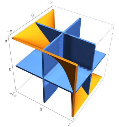
Figure 4.1. On the left, $\Sigma$ for $\Gamma$ a 3-flower (one vertex and three loops), with loop factors $Z_{e_{1}},Z_{e_{2}}$ and $Z_{e_{3}}$ in blue and main factor $Z_{0}$ in orange. On the right, only $Z_{0}^{reg}$. In both plots, $\vec{\kappa}$ range in $\left(-\pi,\pi\right)^{3}$ so that the loop factors are visible.

Theorem 4.53.

If $\Gamma$ is a graph with a bridge $e$ and no loops, then $\Sigma^{reg}$ has two connected components and the bridge extension $\tau_{e}$ (Definition 4.40) is an isometry between the two components.

Proof.

Recall that if a graph has a bridge $e$ we defined its bridge decomposition
$\Gamma\setminus\left\{e\right\}=\Gamma_{1}\sqcup\Gamma_{2}$ with sets of edges $\mathcal{E}_{1}$ and $\mathcal{E}_{2}$ correspondingly and torus coordinates $\vec{\kappa}=\left(\vec{\kappa}_{1},\kappa_{e},\vec{\kappa}_{2}\right)$ such that $\vec{\kappa}_{j}\in\mathbb{T}^{\mathcal{E}_{j}}$. We have shown in Proposition 4.36 that the secular function can be factorized into $F\left(\vec{\kappa}\right)=g_{1}\left(\vec{\kappa}_{1}\right)g_{2}\left(\vec{\kappa}_{2}\right)\left(1-e^{i\left(2\kappa_{e}+\Theta_{1}\left(\vec{\kappa}_{1}\right)+\Theta_{2}\left(\vec{\kappa}_{2}\right)\right)}\right)$. We have defined $Z_{g}:=\left\{\left(\vec{\kappa}_{1},\kappa_{e},\vec{\kappa}_{2}\right)\in\mathbb{T}^{\mathcal{E}}\,\,:\,\,g_{1}\left(\vec{\kappa}_{1}\right)g_{2}\left(\vec{\kappa}_{2}\right)=0\right\}$, and we will now prove that $Z_{g}$ is of positive co-dimension in $\Sigma$. In fact, since $\Sigma^{sing}$ is of positive co-dimension in $\Sigma$, then we only need to prove that $Z_{g}\cap\Sigma^{reg}$ is of positive co-dimension in $\Sigma^{reg}$. As each $\left|g_{i}\right|^{2}$ is a real trigonometric polynomial, by Proposition 4.36, and $Z_{g}\cap\Sigma^{reg}$ is the zero set of the real trigonometric polynomial $\left|g_{1}\right|^{2}\left|g_{2}\right|^{2}$, then by Lemma 4.8 either $Z_{g}\cap\Sigma^{reg}$ contains a connected component of $\Sigma^{reg}$ or it is of positive co-dimension in $\Sigma^{reg}$. Assume by contradiction that $Z_{g}\cap\Sigma^{reg}$ contains a connected component of $\Sigma^{reg}$, say $M$. According to [36] there is a residual set $G\subset\left(\mathbb{R}_{+}\right)^{\mathcal{E}}$, such that for every $\vec{l}\in G$, every eigenvalue of $\Gamma_{\vec{l}}$ is simple with eigenfunction that does not vanish on vertices (here we use the fact that $\Gamma$ has no loops). Since $G$ is and the set of rationally independent edge lengths is residual, then so does their intersection. Let $\vec{l}\in G$ be rationally independent, and let $\left\{f_{n}\right\}_{n=0}^{\infty}$ and $\left\{k_{n}\right\}_{n=0}^{\infty}$ be the eigenfunctions and (square-root) eigenvalues of $\Gamma_{\vec{l}}$. So the sequence $\left\{k_{n}\vec{l}\right\}$ is dense in $\Sigma$ by Theorem 4.32, and in particular there exists $n$ such that $\left\{k_{n}\vec{l}\right\}\in M\subset Z_{g}\cap\Sigma^{reg}$. The characterization of $Z_{g}\cap\Sigma^{reg}$ in Lemma 4.38 implies that the canonical eigenfunction $f_{\left\{k_{n}\vec{l}\right\}}$ vanish on the bridge $e$ and in particular on its vertices, and by Lemma 4.11, so does $f_{n}$. But this is a contradiction to [36] as $\vec{l}\in G$. We conclude that $\dim\left(Z_{g}\right)\leq E-2$.

Let us now define partition the sub-torus $\mathbb{T}^{\mathcal{E}_{1}}\times\mathbb{T}^{\mathcal{E}_{2}}$ into two parts:

(4.90) $$X :=\left\{\left(\vec{\kappa}_{1},\vec{\kappa}_{2}\right)\in\mathbb{T}^{\mathcal{E}_{1}}\times\mathbb{T}^{\mathcal{E}_{2}}\,\,:\,\,g_{1}\left(\vec{\kappa}_{1}\right)g_{2}\left(\vec{\kappa}_{2}\right)\neq 0\right\},\,\,and$$

(4.91) $$X^{c} :=\left\{\left(\vec{\kappa}_{1},\vec{\kappa}_{2}\right)\in\mathbb{T}^{\mathcal{E}_{1}}\times\mathbb{T}^{\mathcal{E}_{2}}\,\,:\,\,g_{1}\left(\vec{\kappa}_{1}\right)g_{2}\left(\vec{\kappa}_{2}\right)=0\right\}.$$

So that $Z_{g}=\left\{\left(\vec{\kappa}_{1},\kappa_{e},\vec{\kappa}_{2}\right)\in\mathbb{T}^{\mathcal{E}}\,\,:\,\,\left(\vec{\kappa}_{1},\vec{\kappa}_{2}\right)\in X^{c}\right\}$ and therefore $\dim\left(X^{c}\right)=\dim\left(Z_{g}\right)-1\leq E-3$. It follows that $X^{c}$ has co-dimension of at least two in $\mathbb{T}^{\mathcal{E}_{1}}\times\mathbb{T}^{\mathcal{E}_{2}}$ and therefore cannot bisect this space, so $X$ is connected. According to Proposition 4.36, $e^{-i\left(\Theta_{1}\left(\vec{\kappa}_{1}\right)+\Theta_{2}\left(\vec{\kappa}_{2}\right)\right)}$ is smooth on $X$ and one can deduce from the decomposition of $F$ that,

$$\Sigma\setminus Z_{g}=\left\{\left(\vec{\kappa}_{1},\kappa_{e},\vec{\kappa}_{2}\right)\in\mathbb{T}^{\mathcal{E}}\,\,:\,\,\left(\vec{\kappa}_{1},\vec{\kappa}_{2}\right)\in X\,\,\text{and}\,\,e^{i2\kappa_{e}}=e^{-i\left(\Theta_{1}\left(\vec{\kappa}_{1}\right)+\Theta_{2}\left(\vec{\kappa}_{2}\right)\right)}\right\}.$$

Define the continuous function $y:X\rightarrow\mathbb{R}/2\pi\mathbb{Z}$ by $e^{iy}=e^{-i\left(\Theta_{1}\left(\vec{\kappa}_{1}\right)+\Theta_{2}\left(\vec{\kappa}_{2}\right)\right)}$. Since $X$ is connected, then so does the graph of the continuous function $y$ (embedded into $\mathbb{T}^{\mathcal{E}}$),

$$\mathrm{Graph}\left(y\right):=\left\{\left(\vec{\kappa}_{1},y,\vec{\kappa}_{2}\right)\in\mathbb{T}^{\mathcal{E}}\,\,:\,\,\left(\vec{\kappa}_{1},\vec{\kappa}_{2}\right)\in X\,\,\text{and}\,\,\,e^{iy}=e^{-i\left(\Theta_{1}\left(\vec{\kappa}_{1}\right)+\Theta_{2}\left(\vec{\kappa}_{2}\right)\right)}\right\}.$$

Notice that $y\left(\kappa_{e}\right)$ given by the equation $e^{i2\kappa_{e}}=e^{iy}$ is two to one, therefore $\Sigma\setminus Z_{g}=\left\{\left(\vec{\kappa}_{1},\kappa_{e},\vec{\kappa}_{2}\right)\,\,:\,\,e^{i2\kappa_{e}}=e^{-i\left(\Theta_{1}\left(\vec{\kappa}_{1}\right)+\Theta_{2}\left(\vec{\kappa}_{2}\right)\right)}\right\}$ has at most two connected components. As $Z_{g}\cap\Sigma^{reg}$ is closed and of positive co-dimension, then $\Sigma\setminus Z_{g}$ is an open dense subset set of $\Sigma^{reg}$, and therefore $\Sigma^{reg}$ has at most two connected components.

Recall that the bridge extension $\tau_{e}$ is an isometry of $\Sigma^{reg}$ as seen in the proof of Lemma 4.42. We will now show that for any point $\vec{\kappa}\in\Sigma^{reg}$, the points $\vec{\kappa}$ and $\tau_{e}\left(\vec{\kappa}\right)$ are not in the same connected component. This will prove that $\Sigma^{reg}$ has at least and therefore exactly two connected components, and that $\tau_{e}$ is an isometry between the two.

It is immediate from the decomposition of $F$ in Proposition 4.36 that $F\circ\tau_{e}=-F$. Since $\tau_{e}$ is a translation, then it commutes with derivatives and therefore $-\nabla F=\nabla\left(F\circ\tau_{e}\right)=\nabla F\circ\tau_{e}$, namely $\nabla F\left(\tau_{e}\left(\vec{\kappa}\right)\right)=-\nabla F\left(\vec{\kappa}\right)$ for all $\vec{\kappa}\in\mathbb{T}^{\mathcal{E}}$. Let $\vec{\kappa}\in\Sigma^{reg}$, according to Lemma 4.20, the non-vanishing components of $\nabla F\left(\vec{\kappa}\right)$ have the same sign as the sign of $p\left(\vec{\kappa}\right)$, and same for $\tau_{e}\left(\vec{\kappa}\right)\in\Sigma^{reg}$. Therefore, $p\left(\tau_{e}\left(\vec{\kappa}\right)\right)=-p\left(\vec{\kappa}\right)$, and since $p$ is real, non-vanishing and continuous on $\Sigma^{reg}$ then $\vec{\kappa}$ and $\tau_{e}\left(\vec{\kappa}\right)$ belongs to different connected components. ∎

Theorem 4.54.

Let $\Gamma$ be a graph with $\left|\mathcal{E}_{loops}\right|>0$ loops, then $\Sigma^{reg}$ has at least $\left|\mathcal{E}_{loops}\right|+1$ connected components. However, $Z_{0}^{reg}$ is connected.

The lower bound on the number of connected components is straightforward from Lemma 4.49. The proof of $Z_{0}^{reg}$ being connected is very similar to that of Theorem 4.53:

Proof.

As discussed in Lemma 4.49, $\Sigma^{reg}=\Sigma_{\mathcal{L}}^{c}\sqcup_{e\in\mathcal{E}_{loops}}\tilde{Z}_{e}$ where each of these sets is a union of connected components of $\Sigma^{reg}$ and has positive measure (so it is not empty). It follows that there must be at least $\left|\mathcal{E}_{loops}\right|+1$ connected components of $\Sigma^{reg}$.

Let $e$ be a distinguished loop and consider the notation $\vec{\kappa}=\left(\kappa_{e},\vec{\kappa}_{\overline{e}}\right)$ where $\vec{\kappa}_{\overline{e}}$ denotes the rest of the entries of $\vec{\kappa}$ which are not $\kappa_{e}$. Consider the decomposition of $U_{\vec{\kappa}}$ according to (4.76), so that $1-U_{\vec{\kappa}}=\left(1-e^{i\hat{\kappa}_{loops}}\right)\oplus\left(1-U_{0}\left(\vec{\kappa}\right)\right)$ where $U_{0}\left(\vec{\kappa}\right)=e^{i\hat{\kappa}_{0}}S_{0}$. As both $e^{i\hat{\kappa}_{loops}}$ and $e^{i\hat{\kappa}_{0}}$ are unitary diagonal with $e^{i\kappa_{e}}$ appearing ones in each of them, then both $\det\left(1-U_{0}\left(\vec{\kappa}\right)\right)$ and $\det\left(1-e^{i\hat{\kappa}_{loops}}\right)$ are polynomials of degree one in $e^{i\kappa_{e}}$. We may define $h_{0}\left(\vec{\kappa}_{\overline{e}}\right)=\Pi_{e^{\prime}\in\mathcal{E}_{loops};\,e^{\prime}\neq e}\left(1-e^{i\kappa_{e^{\prime}}}\right)$ such that $\det\left(1-e^{i\hat{\kappa}_{loops}}\right)=\left(1-e^{i\kappa_{e}}\right)h_{0}\left(\vec{\kappa}_{\overline{e}}\right)$. We may also define $h_{1}$ and $h_{2}$, by

(4.92) $$\det\left(1-U_{0}\left(\vec{\kappa}\right)\right)=h_{2}\left(\vec{\kappa}_{\overline{e}}\right)e^{i\kappa_{e}}+h_{1}\left(\vec{\kappa}_{\overline{e}}\right),$$

such that both $h_{1}$ and $h_{2}$ are polynomials in $\left\{e^{i\kappa_{e^{\prime}}}\right\}_{e^{\prime}\neq e}$ with real coefficients (since $S_{0}$ is real). Therefore,

(4.93) $$F\left(\kappa_{e},\vec{\kappa}_{\overline{e}}\right)= \det\left(U_{\vec{\kappa}}\right)^{\frac{1}{2}}\det\left(1-U_{\vec{\kappa}}\right)$$

(4.94) $$= \left(i^{\left(\beta-1\right)}e^{-i\sum_{e^{\prime}\neq e}\kappa_{e^{\prime}}}\right)e^{-i\kappa_{e}}\det\left(1-U_{\vec{\kappa}}\right)$$

(4.95) $$= \left(i^{\left(\beta-1\right)}e^{-i\sum_{e^{\prime}\neq e}\kappa_{e^{\prime}}}\right)e^{-i\kappa_{e}}\det\left(1-e^{i\hat{\kappa}_{loops}}\right)\det\left(1-U_{0}\left(\vec{\kappa}\right)\right)$$

(4.96) $$= \left(i^{\left(\beta-1\right)}e^{-i\sum_{e^{\prime}\neq e}\kappa_{e^{\prime}}}\right)e^{-i\kappa_{e}}\left(1-e^{i\kappa_{e}}\right)h_{0}\left(\vec{\kappa}_{\overline{e}}\right)\left(h_{2}\left(\vec{\kappa}_{\overline{e}}\right)e^{i\kappa_{e}}+h_{1}\left(\vec{\kappa}_{\overline{e}}\right)\right)$$

(4.97) $$= \left(i^{\left(\beta-1\right)}e^{-i\sum_{e^{\prime}\neq e}\kappa_{e^{\prime}}}\right)\left(1-e^{i\kappa_{e}}\right)h_{0}\left(\vec{\kappa}_{\overline{e}}\right)\left(h_{2}\left(\vec{\kappa}_{\overline{e}}\right)+e^{-i\kappa_{e}}h_{1}\left(\vec{\kappa}_{\overline{e}}\right)\right).$$

Denoting the uni-modular prefactor $c\left(\vec{\kappa}_{\overline{e}}\right)=\left(i^{\left(\beta-1\right)}e^{-i\sum_{e^{\prime}\neq e}\kappa_{e^{\prime}}}\right)$ and suppressing the $\vec{\kappa}_{\overline{e}}$ dependence in $c,h_{0},h_{1}$ and $h_{3}$ for simplicity, this gives:

(4.98) $$F\left(\kappa_{e},\vec{\kappa}_{\overline{e}}\right) =ch_{0}\left(1-e^{i\kappa_{e}}\right)\left(h_{2}+e^{-i\kappa_{e}}h_{1}\right),\,and$$

(4.99) $$\frac{\partial}{\partial\kappa_{e}}F\left(\kappa_{e},\vec{\kappa}_{\overline{e}}\right) =ch_{0}\left(h_{2}\left(1-ie^{i\kappa_{e}}\right)-h_{1}\left(1+ie^{-i\kappa_{e}}\right)\right).$$

One may check that the function $\left(1-e^{ix}\right)\left(A+Be^{-ix}\right)$ is real for all $x\in\mathbb{R}$ if and only if $A=-\overline{B}$. As $F$ is real, $\left|c\right|=1$ and $h_{0}\left(\vec{\kappa}_{\overline{e}}\right)\neq 0$ for any $\vec{\kappa}_{\overline{e}}\in\left(0,2\pi\right)^{\mathcal{E}\setminus e}$ then $\left|h_{2}\right|=\left|h_{1}\right|$ for any $\vec{\kappa}_{\overline{e}}\in\left(0,2\pi\right)^{\mathcal{E}\setminus e}$. This equality extends to $\mathbb{T}^{\mathcal{E}\setminus e}$ by continuity. Let

(4.100) $$X^{c} :=\left\{\vec{\kappa}_{\overline{e}}\in\mathbb{T}^{\mathcal{E}\setminus e}\,\,:\,\,h_{2}\left(\vec{\kappa}_{\overline{e}}\right)=h_{1}\left(\vec{\kappa}_{\overline{e}}\right)=0\right\}$$

(4.101) $$X :=\mathbb{T}^{\mathcal{E}\setminus e}\setminus X=\left\{\vec{\kappa}_{\overline{e}}\in\mathbb{T}^{\mathcal{E}\setminus e}\,\,:\,\,\left|h_{2}\left(\vec{\kappa}_{\overline{e}}\right)\right|=\left|h_{1}\left(\vec{\kappa}_{\overline{e}}\right)\right|\neq 0\right\},\,\,\text{and}$$

(4.102) $$Z_{h} :=\left\{\left(\kappa_{e},\vec{\kappa}_{\overline{e}}\right)\in\mathbb{T}^{\mathcal{E}}\,\,:\,\,\vec{\kappa}_{\overline{e}}\in X^{c}\right\}.$$

Observe that $\left|\frac{\partial}{\partial\kappa_{e}}\det\left(1-U_{0}\left(\vec{\kappa}\right)\right)\right|=\left|h_{2}\left(\vec{\kappa}_{\overline{e}}\right)\right|$ and therefore, by the characterization in (4.79),

(4.103) $$Z_{0}\setminus Z_{h}\subset Z_{0}^{reg}.$$

If $\vec{\kappa}\in Z_{h}\cap\Sigma^{reg}$, namely $h_{1}=h_{2}=0$, then $\frac{\partial}{\partial\kappa_{e}}F=0$ according to (4.99). Then by Lemma 4.20, the amplitudes vector of $f_{\vec{\kappa}}$ satisfies $\left|a_{e}\right|^{2}+\left|a_{\hat{e}}\right|^{2}=0$, and hence $f_{\vec{\kappa}}|_{e}\equiv 0$. Therefore, if $\vec{\kappa}\in\Sigma^{reg}$ and $f_{\vec{\kappa}}$ does not vanish on vertices, then $\vec{\kappa}\notin Z_{h}$ and is also not in any loop factor $Z_{e^{\prime}}$. We may conclude, using the decomposition in Lemma 4.49, that having $f_{\vec{\kappa}}$ does not vanish on vertices implies $\vec{\kappa}\in\Sigma^{reg}\cap Z_{0}\setminus Z_{h}$.

According to [36], if a graph has loops, then there is a residual sets of edge lengths $G\subset\left(\mathbb{R}_{+}\right)^{\mathcal{E}}$ such that for every $\vec{l}\in G$, every eigenvalue of $\Gamma_{\vec{l}}$ is simple and every eigenfunction is either supported on a single loop or does not vanish on vertices. As in the proof of Theorem 4.53, we may choose $\vec{l}\in G$ which is rationally independent, so that the sequence $\left\{k_{n}\vec{l}\right\}_{n=0}^{\infty}$ is dense in $\Sigma^{reg}$. If $f_{n}$ is supported on a loop $e^{\prime}$, then $\left\{k_{n}\vec{l}\right\}\in Z_{e^{\prime}}\cap\Sigma^{reg}=Z_{e^{\prime}}^{reg}$, otherwise, $f_{n}$ does not vanish on any vertex, and so does $f_{\left\{k_{n}\vec{l}\right\}}$ (by Lemma 4.11), so $\left\{k_{n}\vec{l}\right\}\in\Sigma^{reg}\cap Z_{0}\setminus Z_{h}$. Since $Z_{h}$ is the zero set of a real trigonometric polynomial $\left|h_{1}\right|^{2}+\left|h_{2}\right|^{2}=0$ and $Z_{0}^{reg}$ is a real analytic manifold of dimension $E-1$, then the same argument as in the proof of Theorem 4.53 would show that $\dim\left(Z_{h}\cap\Sigma^{reg}\right)\leq E-2$ and therefore $\dim\left(Z_{h}\right)\leq E-2$. It follows that $\dim\left(X^{c}\right)=\dim\left(Z_{h}\right)-1\leq E-3$ which co-dimension of at least two in $\mathbb{T}^{\mathcal{E}\setminus e}$ and therefore $X$ is connected. Define the function $y:X\rightarrow\mathbb{R}/2\pi\mathbb{Z}$ given by $e^{iy}=-\frac{h_{1}\left(\vec{\kappa}_{\overline{e}}\right)}{h_{2}\left(\vec{\kappa}_{\overline{e}}\right)}$ and notice that it is is continuous, so it has a connected graph (embedded into $\mathbb{T}^{\mathcal{E}}$):

$$Graph\left(y\right) :=\left\{\left(y,\vec{\kappa}_{\overline{e}}\right)\in\mathbb{T}^{\mathcal{E}}\,\,:\,\,\vec{\kappa}_{\overline{e}}\in X\,\,\,\text{and}\,\,\,e^{iy}=-\frac{h_{1}\left(\vec{\kappa}_{\overline{e}}\right)}{h_{2}\left(\vec{\kappa}_{\overline{e}}\right)}\right\}$$

$$= \left\{\left(y,\vec{\kappa}_{\overline{e}}\right)\in\mathbb{T}^{\mathcal{E}}\,\,:\,\,\vec{\kappa}_{\overline{e}}\in X\,\,\,\text{and}\,\,\,h_{2}\left(\vec{\kappa}_{\overline{e}}\right)e^{iy}+h_{1}\left(\vec{\kappa}_{\overline{e}}\right)=0\right\}$$

$$= \left\{\left(\kappa_{e},\vec{\kappa}_{\overline{e}}\right)\in\mathbb{T}^{\mathcal{E}}\,\,:\,\,\vec{\kappa}_{\overline{e}}\in X\,\,\,\text{and}\,\,\,\det\left(1-U_{0}\left(\vec{\kappa}\right)\right)=0\right\},$$

$$= Z_{0}\setminus Z_{h}.$$

Therefore $Z_{0}\setminus Z_{h}$ is connected. But it is dense in $Z_{0}^{reg}$ as $Z_{h}$ is of positive co-dimension so therefor $Z_{0}^{reg}$ is connected. ∎

5. generic eigenfunctions

Recall that we define (see Definition 2.20) a generic eigenfunction as an eigenfunction of a simple eigenvalue that satisfies both properties $I$ and $II$. Where an eigenfunction is said to satisfy property $I$ if it does not vanish on vertices, and property $II$ if non of its outgoing derivatives vanish on any interior vertex (see Definition 2.19).

The main goal of this chapter, as discussed in the introduction, is Theorem 5.5 which proves, for two related notions of genericity, that the eigenfunctions we call generic are indeed generic (among the eigenfunctions which are not supported on loops).

The first genericity result for quantum graphs is duo to Friedlander, who proved in [67] that given a graph $\Gamma$ there is a residual set of edge length $G\subset\mathbb{R}_{+}^{\mathcal{E}}$ such that for any $\vec{l}\in G$, the spectrum of $\Gamma_{\vec{l}}$ is simple (i.e every eigenvalue is simple). This result was generalized by Berkolaiko and Liu as follows:

Theorem 5.1.

[36, Theorem 3.6] Given a graph $\Gamma$ there is a residual set of edge lengths $G\subset\mathbb{R}_{+}^{\mathcal{E}}$ such that for any $\vec{l}\in G$, the spectrum of $\Gamma_{\vec{l}}$ is simple. Moreover, every eigenfunction is either supported on a single loop (if such exists) or satisfies Property $I$.

In [8, Proposition A.1] it was shown that the non-explicit residual set $G$ can be replaced by the explicit residual set of rationally independent edge lengths, if we restrict the discussion to ‘almost every eigenvalue and eigenfunction’ (in the sense of a sub-sequence of density one). In order to state it, let us define the following index sets:

Definition 5.2.

Given a standard graph $\Gamma_{\vec{l}}$ with (square-root) eigenvalues and eigenfunctions $\left\{k_{n}\right\}_{n=0}^{\infty}$ and $\left\{f_{n}\right\}_{n=0}^{\infty}$, we define the following index sets:

(5.1) $$\mathcal{S}:=\left\{n\in\mathbb{N}~{}:~{}k_{n}\>\>\text{is simple}\right\},$$

(5.2) $$\mathcal{P}_{I} :=\left\{n\in\mathcal{S}\,\,:\,\,f_{n}\,\,\text{satisfies property I}\right\},$$

(5.3) $$\mathcal{P}_{II} :=\left\{n\in\mathcal{S}\,\,:\,\,f_{n}\,\,\text{satisfies property II}\right\},\,\,\text{and}$$

(5.4) $$\mathcal{L} :=\left\{n\in\mathcal{S}\,\,:\,\,f_{n}\,\,\text{is supported on a loop}\right\}.$$

Where $\mathcal{L}=\emptyset$ if $\Gamma_{\vec{l}}$ has no loops. The index set of generic eigenfunction $\mathcal{G}$ (see Definition 2.20) can be written as

(5.5) $$\mathcal{G}=\mathcal{P}_{I}\cap\mathcal{P}_{II}.$$

Remark 5.3.

As discussed in Remark 2.21, these sets are $\vec{l}$ dependent, but are independent of the choice of eigenfunctions $\left\{f_{n}\right\}_{n=0}^{\infty}$. This is because different choices of $L^{2}$ basis of eigenfunctions may differ only on eigenspaces of non-simple eigenvalues, and so subsets of $\mathcal{S}$ are independent of this choice. It is not hard to deduce that $\mathcal{L}$ and $\mathcal{P}_{I}\cup\mathcal{P}_{II}$ are disjoint and in particularly, $\mathcal{L}$ and $\mathcal{G}$ are disjoint.

A Venn diagram of these index sets is presented Figure 5.1 for visualization.

Figure 5.1. A Venn diagram of the index sets. Where $I$ and $II$ stands for $\mathcal{P}_{I}$ and $\mathcal{P}_{II}$. ‘Simple’ and ‘Generic’ stands for $\mathcal{S}$ and $\mathcal{G}$, and ‘Supported on loops’ stands for $\mathcal{L}$. The outer white region stands for the indices of the non-simple eigenvalues, namely $\mathbb{N}\setminus\mathcal{S}$.

Theorem 5.1 can be written, using this terminology, as the existence of a residual set $G$ such that for any $\vec{l}\in G$, $\mathbb{N}=\mathcal{S}=\mathcal{P}_{I}\sqcup\mathcal{L}$. Using the notations as above, the modification of [8, Proposition A.1] can be written as follows.

Theorem 5.4.

[8, Proposition A.1] If $\vec{l}$ is rationally independent with total length $L$, then $\mathcal{S}$, $\mathcal{L}$ and $\mathcal{P}_{I}$ have densities given by

$$d\left(\mathcal{S}\right) =1,$$

$$d\left(\mathcal{L}\right) =\frac{1}{2}\frac{\sum_{e\in\mathcal{E}_{loops}}l_{e}}{L},\,\,\text{and}$$

$$d\left(\mathcal{P}_{I}\right) =1-d\left(\mathcal{L}\right)=1-\frac{1}{2}\frac{\sum_{e\in\mathcal{E}_{loops}}l_{e}}{\sum_{e\in\mathcal{E}}l_{e}}\geq\frac{1}{2}.$$

We will now prove the following theorem that generalizes both [8, Proposition A.1] and [36, Theorem 3.6] from $\mathcal{P}_{I}$ to $\mathcal{G}$:

Theorem 5.5.

[5] Given a graph $\Gamma$,

1. There is a residual set of edge lengths $G\subset\mathbb{R}_{+}^{\mathcal{E}}$ such that for any $\vec{l}\in G$,

   (5.6) $$\mathbb{N}=\mathcal{S}=\mathcal{G}\sqcup\mathcal{L}.$$

   That is, the spectrum of $\Gamma_{\vec{l}}$ is simple, and every eigenfunction is either supported on a loop or generic.

2. If $\Gamma_{\vec{l}}$ is a standard graph with $\vec{l}$ rationally independent, then $\mathcal{G}$ has density, and it is given by

   (5.7) $$d\left(\mathcal{G}\right)=1-d\left(\mathcal{L}\right)=1-\frac{1}{2}\frac{\sum_{e\in\mathcal{E}_{loops}}l_{e}}{\sum_{e\in\mathcal{E}}l_{e}}.$$

   Namely almost every eigenfunction is either supported on a loop or generic.

Remark 5.6.

In the context of Neumann domains on manifolds, one needs to restrict the discussion to eigenfunctions which are Morse functions as discussed in [17]. These are eigenfunctions with full rank Hessian at every critical point. On a standard graph, an eigenfunction $f$ is not Morse if there is an edge $e$ with an interior point $x_{0}\in e$ such that $f^{\prime}\left(x_{0}\right)=f^{\prime\prime}\left(x_{0}\right)=0$. If $f$ is not the constant eigenfunction, then by Definition 2.16, $f|_{e}\equiv 0$. Therefore, on a standard graph, Morse eigenfunctions are non-constant eigenfunctions such that $f|_{e}\not\equiv 0$ for any edge $e$. We conclude that every generic eigenfunction is Morse and every Morse eigenfunction is not supported on a loop. Therefore, by Theorem 5.5, almost every eigenfunction is either supported on a loop or both Morse and generic.

5.1. Outline of the proof.

The proof of Theorem 5.5 has the following sequence of deductions:

1. We show that Theorem 5.5 follows from:

   (5.8) $$\forall\vec{l}\in\left(\mathbb{R}_{+}\right)^{\mathcal{E}}\,\,\mu_{\vec{l}}\left(\Sigma_{\mathcal{G}}\sqcup\Sigma_{\mathcal{L}}\right)=1.$$

2. We show that if (5.8) fails for some graph $\Gamma$, then there is an open set $O\subset\Sigma^{reg}$ on which

   (5.9) $$\exists v\in\mathcal{V}_{in},e\in\mathcal{E}_{v}\,\,\,s.t\,\,\forall\vec{\kappa}\in O,\,\,\partial_{e}f_{\vec{\kappa}}\left(v\right)=0\,\,\text{and }\,\,f_{\vec{\kappa}}\left(v\right)\neq 0.$$

3. We show that if there exists such an open set $O$ and a pair $v,e$ as above, then

   1. In the case that $\Gamma$ has loops and\or bridges, every canonical eigenfunction would satisfy $\partial_{e}f_{\vec{\kappa}}\left(v\right)=0$.

   2. In the case that $\Gamma$ has no loops and no bridges, we can construct a different graph $\tilde{\Gamma}$ with interior vertex $u_{1}$ and boundary vertex $u_{2}$ such that every canonical eigenfunction of $\tilde{\Gamma}$ would satisfy $\left|f_{\vec{\kappa}}\left(u_{1}\right)\right|=\left|f_{\vec{\kappa}}\left(u_{2}\right)\right|$.

4. We contradict (a) by proving that for every graph $\Gamma$ and any choice of $v\in\mathcal{V}_{in}$ and $e\in\mathcal{E}_{v}$ there exists $\vec{\kappa}\in\Sigma^{reg}$ for which $\partial_{e}f_{\vec{\kappa}}\left(v\right)\neq 0$. We contradict (b) by proving that if $\Gamma$ is a graph with boundary, then for any boundary vertex $u_{1}$ and interior vertex $u_{2}$ there exists $\vec{\kappa}\in\Sigma^{reg}$ for which $\left|f_{\vec{\kappa}}\left(u_{1}\right)\right|\neq\left|f_{\vec{\kappa}}\left(u_{1}\right)\right|$. This proves that no such $O$ exists, which proves that (5.8) is not false, which proves Theorem 5.5.

In order to prove Theorem 5.5, we first need to relate all properties discussed above to subsets of the secular manifolds, and discuss the properties of these subsets:

5.2. Special subsets of the secular manifold

Definition 5.7.

Let $\Gamma$ be a graph and consider the regular part of the secular manifold $\Sigma^{reg}$. We define the following subsets of $\Sigma^{reg}$:

(5.10) $$\Sigma_{I}:=\left\{\vec{\kappa}\in\Sigma^{reg}\,\,:\,\,f_{\vec{\kappa}}\,\,\text{satisfy property I}\right\},$$

and similarly $\Sigma_{II}$ with property II. We define the generic part by:

(5.11) $$\Sigma_{\mathcal{G}}:=\left\{\vec{\kappa}\in\Sigma^{reg}\,\,:\,\,f_{\vec{\kappa}}\,\,\text{is generic}\right\},$$

so that $\Sigma_{\mathcal{G}}=\Sigma_{I}\cap\Sigma_{II}$.

Remark 5.8.

Recall that by Lemma 4.49, if a graph has loops, then

$$\Sigma^{reg}=\Sigma_{\mathcal{L}}\sqcup\Sigma_{\mathcal{L}}^{c},$$

where

$$\Sigma_{\mathcal{L}} :=\left\{\vec{\kappa}\in\Sigma^{reg}\,\,:\,\,f_{\vec{\kappa}}\,\,\text{is supported on a loop}\right\},\,\,\text{and}$$

$$\Sigma_{\mathcal{L}}^{c} =Z_{0}^{reg}\cap\Sigma^{reg}.$$

See Definition 4.47 for $Z_{0}^{reg}$. By their definitions, both $\Sigma_{I}$ and $\Sigma_{II}$ are subsets of $\Sigma_{\mathcal{L}}^{c}$ and so does their intersection $\Sigma_{\mathcal{G}}$.

According to Lemma 4.49 both $\Sigma_{\mathcal{L}}$ and $\Sigma_{\mathcal{L}}^{c}$ are unions of connected components of $\Sigma^{reg}$. As such, they are both closed and open in $\Sigma^{reg}$ (since its a manifold) and are Jordan according to Remark 4.33.

Remark 5.9.

If a graph has no loops we say that $\Sigma_{\mathcal{L}}=\emptyset$ and $\Sigma_{\mathcal{L}}^{c}=\Sigma^{reg}$. In fact, the graph has no loops if and only if $\Sigma_{\mathcal{L}}=\emptyset$, as Lemma 4.49 says that for a graph with at least one loop $\Sigma_{\mathcal{L}}$ has positive measure.

The index sets Venn diagram can be used for these sets as well, as presented in Figure 5.2.

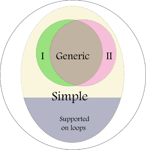
Figure 5.2. A Venn diagram of the partition of $\Sigma$ to subsets. Where $I$ and $II$ stands for $\Sigma_{I}$ and $\Sigma_{II}$. ‘Simple’ stands for $\Sigma^{reg}$ and ‘Generic’ stands for $\Sigma_{\mathcal{G}}$. ‘Supported on loops’ stands for $\Sigma_{\mathcal{L}}$. The outer white region stands for $\Sigma^{sing}$.

The relation to the index sets in Definition 5.2 is given by:

Lemma 5.10.

Given a standard graph $\Gamma_{\vec{l}}$ with (square-root) eigenvalues and eigenfunctions $\left\{k_{n}\right\}_{n=0}^{\infty}$ and $\left\{f_{n}\right\}_{n=0}^{\infty}$, then

(5.12) $$\mathcal{S} =\left\{n\in\mathbb{N}\,\,:\,\,\left\{k_{n}\vec{l}\right\}\in\Sigma^{reg}\right\}.$$

(5.13) $$\mathcal{P}_{I} :=\left\{n\in\mathbb{N}\,\,:\,\,\left\{k_{n}\vec{l}\right\}\in\Sigma_{I}\right\}.$$

(5.14) $$\mathcal{P}_{II} :=\left\{n\in\mathbb{N}\,\,:\,\,\left\{k_{n}\vec{l}\right\}\in\Sigma_{II}\right\}.$$

(5.15) $$\mathcal{G} :=\left\{n\in\mathbb{N}\,\,:\,\,\left\{k_{n}\vec{l}\right\}\in\Sigma_{\mathcal{G}}\right\}.$$

(5.16) $$\mathcal{L} :=\left\{n\in\mathbb{N}\,\,:\,\,\left\{k_{n}\vec{l}\right\}\in\Sigma_{\mathcal{L}}\right\}.$$

Proof.

The characterizations of $\mathcal{S}$ in terms of $\Sigma^{reg}$ and $\mathcal{L}$ in terms of $\Sigma_{\mathcal{L}}$ are straightforward from their definitions. According to Lemma 4.11, an eigenfunction $f_{n}$ of a simple eigenvalue $k_{n}$ satisfies property I or II if and $f_{\vec{\kappa}}$ satisfies property I or II, for $\vec{\kappa}=\left\{k_{n}\vec{l}\right\}$. The relations between $\mathcal{P}_{I},\,\mathcal{P}_{II}$ and $\mathcal{G}$ to $\Sigma_{I},\,\Sigma_{II}$ and $\Sigma_{\mathcal{G}}$ follows. ∎

Definition 5.11.

We define the following zero sets on $\Sigma_{\mathcal{L}}^{c}$:

(5.17) $$\forall v\in\mathcal{V}\,\,\,\,\,\,Z_{v}:= \left\{\vec{\kappa}\in\Sigma_{\mathcal{L}}^{c}\,\,:\,\,f_{\vec{\kappa}}\left(v\right)=0\right\},$$

(5.18) $$\forall v\in\mathcal{V}_{in},\,\forall e\in\mathcal{E}_{v}\,\,\,\,\,Z_{v,e}:= \left\{\vec{\kappa}\in\Sigma_{\mathcal{L}}^{c}\,\,:\,\,\partial_{e}f_{\vec{\kappa}}\left(v\right)=0\right\},\,\,\,\text{and}$$

(5.19) $$\forall v,u\in\mathcal{V}\,\,\,\,\,Z_{v,u}:= \left\{\vec{\kappa}\in\Sigma_{\mathcal{L}}^{c}\,\,:\,\,f_{\vec{\kappa}}\left(v\right)^{2}-f_{\vec{\kappa}}\left(u\right)^{2}=0\right\}.$$

We will refer to these subsets as the $Z_{*}$’s.

Remark 5.12.

Observe that $\Sigma_{\mathcal{G}}$ is the complement (in $\Sigma_{\mathcal{L}}^{reg}$) of the union:

(5.20) $$\Sigma_{\mathcal{L}}\cup_{v\in\mathcal{V}_{in},e\in\mathcal{E}_{v}}Z_{v,e}\cup_{u\in\mathcal{V}}Z_{u}.$$

Since $\Sigma_{\mathcal{L}}^{c}$ is a real analytic manifold (as a union of connected components of $\Sigma^{reg}$) and each of the $Z_{*}$’s subsets is the zero set of either $f_{\vec{\kappa}}\left(v\right)^{2},\,\,\partial_{e}f_{\vec{\kappa}}\left(v\right)^{2}$ or $f_{\vec{\kappa}}\left(v\right)^{2}-f_{\vec{\kappa}}\left(u\right)^{2}$ which are real analytic according to (4.11), then we can apply Lemma 4.8 for zero sets of real analytic functions and conclude that:

Lemma 5.13.

Let $A\subset\Sigma_{\mathcal{L}}^{c}$ be a finite union of $Z_{*}$’s as in Definition 5.11, and denote its complement by $A^{c}=\Sigma_{\mathcal{L}}^{c}\setminus A$. Then $A^{c}$ is an open Jordan subset of $\Sigma$. Moreover, if we assume that $A$ has zero co-dimension in $\Sigma_{\mathcal{L}}^{c}$, then

1. If $\Gamma$ has at least one loop, then $A=\Sigma_{\mathcal{L}}^{c}$.

2. If $\Gamma$ has no loops but has at least one bridge (including tail) then $A=\Sigma^{reg}=\Sigma_{\mathcal{L}}^{c}$.

3. If $\Gamma$ has no loops and no bridges, then $A$ contains every connected component of $\Sigma^{reg}$ on which it has zero co-dimension.

Proof.

Let $A=\cup_{j=1}^{N}Z_{h_{j}}$ where each $h_{j}$ is either $f_{\vec{\kappa}}\left(v\right)^{2},\,\,\partial_{e}f_{\vec{\kappa}}\left(v\right)^{2}$ or $f_{\vec{\kappa}}\left(v\right)^{2}-f_{\vec{\kappa}}\left(u\right)^{2}$ for some $v,u\in\mathcal{V}$ and $e\in\mathcal{E}_{v}$ and $Z_{h_{j}}$ is the zero set of $h_{j}$ in $\Sigma_{\mathcal{L}}^{c}$. Let $h\left(\vec{\kappa}\right)=\Pi_{j=1}^{N}h_{j}\left(\vec{\kappa}\right)$ so that its zero set $Z_{h}$ is equal to $A$. According to Lemma (4.11), each $h_{j}$ is real analytic and therefore $h$ is real analytic. If $\Gamma$ has loops, then according to Lemma 4.51 each $h_{j}$ can extended to a real analytic function $\tilde{h}_{j}$ on $Z_{0}^{reg}$. Therefore $\tilde{h}$, the product of theses $\tilde{h}_{j}$’s, is a real analytic extension of $h$ from $\Sigma_{\mathcal{L}}^{c}$ to $Z_{0}^{reg}$. Since $Z_{0}^{reg}$ is connected by Theorem 4.54, then we may use Lemma 4.8 and the assumption that $Z_{h}$ has zero co-dimension in $\Sigma_{\mathcal{L}}^{c}$ to conclude that $\tilde{h}$ vanish on all of $Z_{0}^{reg}$ and so $Z_{h}=\Sigma_{\mathcal{L}}^{c}$.

Now assume that $\Gamma$ has no loops, namely $\Sigma^{reg}=\Sigma_{\mathcal{L}}^{c}$, and let $M$ be a connected component of $\Sigma^{reg}$ such that $Z_{h}\cap M$ has zero co-dimension in $M$. Such $M$ exists by the assumption that $Z_{h}$ has zero co-dimension in $\Sigma_{\mathcal{L}}^{c}$. Since $M$ is a connected real analytic manifold and $h$ is a real analytic function on $M$ whose zero set is $Z_{h}\cap M$, then by Lemma 4.8 $M\subset Z_{h}$.

If $\Gamma$ has a bridge $e^{\prime}$ and $\tau_{e^{\prime}}$ is the bridge extension (see Definition 4.40), then according to Theorem 4.53, $\Sigma^{reg}=M\sqcup\tau_{e^{\prime}}\left(M\right)$. By Lemma 4.42, the functions $f_{\vec{\kappa}}\left(v\right)^{2},\,\,\partial_{e}f_{\vec{\kappa}}\left(v\right)^{2}$ and $f_{\vec{\kappa}}\left(v\right)^{2}-f_{\vec{\kappa}}\left(u\right)^{2}$ are $\tau_{e^{\prime}}$ invariant, and therefore so does every $h_{j}$. It follows that $h$ is $\tau_{e^{\prime}}$ invariant and so $\tau_{e^{\prime}}\left(Z_{h}\right)=Z_{h}$. As we showed that $M\subset Z_{h}$, then so does $\tau_{e^{\prime}}\left(M\right)\subset Z_{h}$ which means that $\Sigma^{reg}=Z_{h}$.

It is left to prove that $A^{c}$ is an open Jordan subset of $\Sigma$ for both cases where $A$ for both cases where $A$ has zero or positive co-dimension in $\Sigma_{\mathcal{L}}^{c}$. Since $A$ is the zero set of $h$, then it is closed and therefore $A^{c}=\Sigma_{\mathcal{L}}^{c}\setminus A$ is open and its boundary is given by $\partial A^{c}\subset\partial A\cup\partial\Sigma_{\mathcal{L}}^{c}$. Since $\Sigma_{\mathcal{L}}^{c}$ is a union of connected components of $\Sigma^{reg}$ then $\partial\Sigma_{\mathcal{L}}^{c}\subset\Sigma^{sing}$ and is therefore of measure zero for any $\mu_{\vec{l}}$. It is thus left to prove that $\partial A$ is of measure zero. If $A$ has positive co-dimension in $\Sigma_{\mathcal{L}}^{c}$, then $\partial A$ also has positive co-dimension (since $A$ was closed in $\Sigma^{reg}$) and has measure zero for any $\mu_{\vec{l}}$. Assume that $A$ has zero co-dimension, and let $M$ be a connected component of $\Sigma_{\mathcal{L}}^{c}$. If $A\cap M$ has positive co-dimension in $M$, then $\partial A\cap M$ has measure zero by the same argument as above. In the case that $A\cap M$ has zero co-dimension in $M$, then we have showed that $M\subset A$ in which case $\partial A\cap M=\emptyset$. Since $\Sigma_{\mathcal{L}}^{c}$ has at most a countable number of connected components, each intersecting $\partial A$ in a measure zero set, then $\partial A\cap\Sigma_{\mathcal{L}}^{c}$ is of measure zero. As $\partial A\subset\Sigma_{\mathcal{L}}^{c}\cup\Sigma^{sing}$ then $\partial A$ is of measure zero and we are done. ∎

A similar result holds for the complements of the $\Sigma^{reg}$ subsets in Definition 5.7:

Corollary 5.14.

The subsets $\Sigma_{I},\,\Sigma_{II}$ and $\,\Sigma_{\mathcal{G}}$, are open and Jordan in $\Sigma$.

Proof.

Denote the complements of the above sets in $\Sigma_{\mathcal{L}}^{c}$ by $\Sigma_{I}^{c},\,\Sigma_{II}^{c}$ and $\Sigma_{\mathcal{G}}^{c}$. By their definition,

$$\Sigma_{I}^{c} =\cup_{v\in\mathcal{V}}Z_{v},$$

$$\Sigma_{II}^{c} =\cup_{v\in\mathcal{V}_{in}}\cup_{e\in\mathcal{E}_{v}}Z_{v,e},\,\,\text{and}$$

$$\Sigma_{\mathcal{G}}^{c} =\Sigma_{II}^{c}\cup\Sigma_{I}^{c}.$$

The result now follows from Lemma 5.13. ∎

The following is a corollary of the above together with Lemma 5.10 and Theorem 4.32:

Corollary 5.15.

If $\Gamma_{\vec{l}}$ is a standard graph with $\vec{l}$ rationally independent, then the index sets $\mathcal{S},\,\mathcal{L},\,\mathcal{P}_{I},\,\mathcal{P}_{II}$ and $\mathcal{G}$ have densities, and they are given by

(5.21) $$d\left(\mathcal{S}\right) =\mu_{\vec{l}}\left(\Sigma^{reg}\right)=1,$$

(5.22) $$d\left(\mathcal{L}\right) =\mu_{\vec{l}}\left(\Sigma_{\mathcal{L}}\right),$$

(5.23) $$d\left(\mathcal{P}_{I}\right) =\mu_{\vec{l}}\left(\Sigma_{I}\right),$$

(5.24) $$d\left(\mathcal{P}_{II}\right) =\mu_{\vec{l}}\left(\Sigma_{II}\right),\,\,\text{and}$$

(5.25) $$d\left(\mathcal{G}\right) =\mu_{\vec{l}}\left(\Sigma_{\mathcal{G}}\right).$$

Proof.

In every equality above, the RHS is the BG-measure of a set $\Sigma_{*}$ that was shown to be Jordan in Corollary 5.14 or Remark 5.8, and the LHS is the density of an index set $\mathbb{N}_{*}=\left\{n\in\mathbb{N}\,\,:\,\,\left\{k_{n}\vec{l}\right\}\in\Sigma_{*}\right\}$ according to lemma 5.10. As $\vec{l}$ is rationally independent, then according to Theorem 4.32, $d\left(\mathbb{N}_{*}\right)=\mu_{\vec{l}}\left(\Sigma_{*}\right)$, which concludes the proof. ∎

5.3. Proof of Theorem 5.5.

As discussed in the outline, the first deduction is the following lemma:

Lemma 5.16.

The statement

(5.26) $$\forall\vec{l}\in\left(\mathbb{R}_{+}\right)^{\mathcal{E}}\,\,\,\mu_{\vec{l}}\left(\Sigma_{\mathcal{G}}\sqcup\Sigma_{\mathcal{L}}\right)=1,$$

implies Theorem 5.5.

Proof.

By Lemma 4.49, $\mu_{\vec{l}}\left(\tilde{Z}_{e}\right)=\frac{l_{e}}{2L}$ for every loop $e$ and every $\vec{l}\in\left(\mathbb{R}_{+}\right)^{\mathcal{E}}$. Therefore,

$$\mu_{\vec{l}}\left(\Sigma_{\mathcal{L}}\right)=\sum_{e\in\mathcal{E}_{loops}}\mu_{\vec{l}}\left(Z_{e}^{reg}\right)=\frac{1}{2}\frac{\sum_{e\in\mathcal{E}_{loops}}l_{e}}{L}.$$

If $\vec{l}$ is rationally independent, then by Corollary 5.15,

(5.27) $$d\left(\mathcal{G}\right)=\mu_{\vec{l}}\left(\Sigma_{\mathcal{G}}\right),\,\,\,d\left(\mathcal{L}\right)=\mu_{\vec{l}}\left(\Sigma_{\mathcal{L}}\right),\,\,\text{and }\,\,d\left(\mathcal{S}\right)=\mu_{\vec{l}}\left(\Sigma^{reg}\right).$$

So Theorem 5.5 (2) now follows from (5.26).

In order to prove Theorem 5.5 (1), assume that (5.26) holds. As seen in the proof of Corollary 5.14, $\Sigma_{\mathcal{G}}^{c}$ the complement of $\Sigma_{\mathcal{G}}$ in $\Sigma_{\mathcal{L}}^{c}$ is a finite union of $Z_{*}$’s and so by Lemma 5.13 is is either of positive co-dimension in $\Sigma^{reg}$ or it contains a connected component of $\Sigma^{reg}$. According to (5.26),

$$\mu_{\vec{l}}\left(\Sigma_{\mathcal{G}}^{c}\right)=\mu_{\vec{l}}\left(\Sigma^{reg}\right)-\mu_{\vec{l}}\left(\Sigma_{\mathcal{G}}\sqcup\Sigma_{\mathcal{L}}\right)=0,$$

and as $\mu_{\vec{l}}$ is strictly positive on open sets (see Remark 4.31), then $\Sigma_{\mathcal{G}}^{c}$ does not contain any connected component of $\Sigma^{reg}$ and is therefore of positive co-dimension in $\Sigma^{reg}$. Namely, $\dim\left(\Sigma^{reg}\setminus\left(\Sigma_{\mathcal{G}}\sqcup\Sigma_{\mathcal{L}}\right)\right)\leq E-2$. By adding $\Sigma^{sing}$ which is also of positive co-dimension in $\Sigma$, we get $\dim\left(\Sigma\setminus\left(\Sigma_{\mathcal{G}}\sqcup\Sigma_{\mathcal{L}}\right)\right)\leq E-2$. As $\Sigma$ is closed in $\mathbb{T}^{\mathcal{E}}$ and $\Sigma_{\mathcal{G}}\sqcup\Sigma_{\mathcal{L}}$ in open in $\Sigma$, then $\Sigma\setminus\left(\Sigma_{\mathcal{G}}\sqcup\Sigma_{\mathcal{L}}\right)$ is closed in $\mathbb{T}^{\mathcal{E}}$. Denote the set $\tilde{B}:=\left\{\vec{l}\in\mathbb{R}^{\mathcal{E}}\,\,:\,\,\left\{\vec{l}\right\}\in\Sigma\setminus\left(\Sigma_{\mathcal{G}}\sqcup\Sigma_{\mathcal{L}}\right)\right\}$, which is the lift of $\Sigma\setminus\left(\Sigma_{\mathcal{G}}\sqcup\Sigma_{\mathcal{L}}\right)$ from $\mathbb{R}^{\mathcal{E}}/2\pi\mathbb{Z}^{\mathcal{E}}$ to $\mathbb{R}^{\mathcal{E}}$. Then $\tilde{B}$ is closed with $\dim\left(\tilde{B}\right)\leq E-2$. Consider the “bad” subset of edge lengths $B\subset\left(\mathbb{R}_{+}\right)^{\mathcal{E}}$ given by

$$B:=\left\{\vec{l}\in\left(\mathbb{R}_{+}\right)^{\mathcal{E}}\,\,:\,\,\exists t>0\,\,\text{s.t}\,\,\,t\vec{l}\in\tilde{B}\right\}.$$

It is the cone of the restriction $\tilde{B}\cap\left(\mathbb{R}_{+}\right)^{\mathcal{E}}$, which is closed in $\left(\mathbb{R}_{+}\right)^{\mathcal{E}}$, and is therefore closed and of dimension $\dim\left(B\right)\leq\dim\left(\tilde{B}\cap\left(\mathbb{R}_{+}\right)^{\mathcal{E}}\right)+1\leq E-1$. It is therefore closed and nowhere dense. Hence, its complement, the “good” set $G=\left(\mathbb{R}_{+}\right)^{\mathcal{E}}\setminus B$ is residual. By definition, if $\vec{l}\in G$, then for every $k>0$ such that $\left\{k\vec{l}\right\}\in\Sigma$ we get that $\left\{k\vec{l}\right\}\in\Sigma_{\mathcal{G}}\sqcup\Sigma_{\mathcal{L}}$ which according to Lemma 5.10 proves 5.5 (1). ∎

Remark 5.17.

The argument above is a machinery showing that every property of a standard graph, that is described by a subset $\Sigma_{*}\subset\Sigma$ whose complement has positive co-dimension, is generic in both senses described above.

The second deduction is the following lemma:

Lemma 5.18.

If $\Gamma$ is such that $\mu_{\vec{l}}\left(\Sigma_{\mathcal{G}}\sqcup\Sigma_{\mathcal{L}}\right)<1$ for some $\vec{l}\in\left(\mathbb{R}_{+}\right)^{\mathcal{E}}$, then there exists an interior vertex $v\in\mathcal{V}_{in}$ and edge $e\in\mathcal{E}_{v}$ such that $Z_{v,e}\setminus Z_{v}$ contains an open set.

Proof.

Let $G$ be the residual set in Theorem 5.1, and let $G^{\prime}$ be its (residual) intersection with the set of rationally independent edge lengths. Let $\vec{l}\in G^{\prime}$, then as $\vec{l}\in G$, $d\left(\mathcal{P}_{I}\right)=1-d\left(\mathcal{L}\right)$ according to Theorem 5.1. Since $\vec{l}$ is also rationally independent, Corollary 5.15 gives,

(5.28) $$\mu_{\vec{l}}\left(\Sigma_{I}\right)=d\left(\mathcal{P}_{I}\right)=1-d\left(\mathcal{L}\right)=1-\mu_{\vec{l}}\left(\Sigma_{\mathcal{L}}\right).$$

Since $G^{\prime}$ is dense in $\mathbb{R}_{+}^{\mathcal{E}}$ and $\mu_{\vec{l}}$ is continuous in $\vec{l}$ (immediate from Definition 4.30), then $\mu_{\vec{l}}\left(\Sigma_{I}\right)=1-\mu_{\vec{l}}\left(\Sigma_{\mathcal{L}}\right)$ for any $\vec{l}$.

As we assumed that $\mu_{\vec{l}}\left(\Sigma_{\mathcal{G}}\right)+\mu_{\vec{l}}\left(\Sigma_{\mathcal{L}}\right)<1=\mu_{\vec{l}}\left(\Sigma_{I}\right)+\mu_{\vec{l}}\left(\Sigma_{\mathcal{L}}\right)$ then $\mu_{\vec{l}}\left(\Sigma_{\mathcal{G}}\right)<\mu_{\vec{l}}\left(\Sigma_{I}\right)$ which means that $\mu_{\vec{l}}\left(\Sigma_{I}\setminus\Sigma_{\mathcal{G}}\right)=\mu_{\vec{l}}\left(\Sigma_{I}\setminus\Sigma_{II}\right)>0$. The set $\Sigma_{I}\setminus\Sigma_{II}$ is a union of sets of the form $Z_{v,e}\setminus Z_{v}$ and so if it has positive measure, then there must be at least one $Z_{v,e}\setminus Z_{v}$ set which is not of positive co-dimension. According to Lemma 5.13, we conclude that there is a connected component $M$ of $\Sigma^{reg}$ contained in $Z_{v,e}$ on which $Z_{v}\cap M$ is a closed set of positive co dimension. Hence $M\cap Z_{v,e}\setminus Z_{v}$ is open (and dense in $M$). ∎

The third deduction requires the notion of splitting a vertex. If $v$ is an interior vertex of $\Gamma$ of $\mathrm{deg}(v)>3$ and $e\in\mathcal{E}_{v}$ is not a bridge, then we define $\tilde{\Gamma}$ as the graph obtained by splitting $v$ into two vertices $v_{1}$ and $v_{2}$ such that $v_{1}$ is only connected to $e$ and thus $v_{2}\in\partial\tilde{\Gamma}$, and $v_{2}$ is connected to the remaining edges in $\mathcal{E}_{v}\setminus\left\{e\right\}$. See Figure 5.3 for example. In Appendix C we discuss this process and the relations between of the secular manifolds of $\Gamma$ and $\tilde{\Gamma}$, which we will use in the proof of the next lemma.

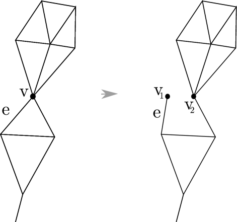
Figure 5.3. On the left, a graph $\Gamma$ with interior vertex $v$ of $\mathrm{deg}(v)=5$ and edge $e\in\mathcal{E}_{v}$ which is not a bridge. On the right, $\tilde{\Gamma}$ obtained by splitting $v$ into $v_{1}$ and $v_{2}$ such that $v_{1}$ is connected to $e$ and has $\mathrm{deg}(v_{1})=1$ and $v_{2}$ is connected to the remaining $\mathcal{E}_{v}\setminus e$ and has $\mathrm{deg}(v_{2})=4$.

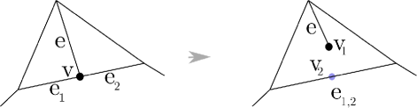
Figure 5.4. On the left, a graph with interior vertex $v$ of $\mathrm{deg}(v)=3$ and $\mathcal{E}_{v}=\left\{e,e_{1},e_{2}\right\}$ such that $e$ is not a bridge. On the right, the graph obtained by splitting $v$ into $v_{1}$ and $v_{2}$ such that $v_{1}$ is connected to $e$ and has $\mathrm{deg}(v_{1})=1$ and $v_{2}$ is considered as an interior vertex of the new edge $e_{1,2}$ which is the concatenation of $e_{1}$ and $e_{2}$.

Lemma 5.19.

Let $\Gamma$ be a graph and assume there exists an interior vertex $v\in\mathcal{V}_{in}$ with an edge $e\in\mathcal{E}_{v}$ such that $Z_{v,e}\setminus Z_{v}$ contains an open set in $\Sigma^{reg}$. Then,

1. If $\Gamma$ has loops or bridges, then for any $\vec{\kappa}\in\Sigma^{reg}$ either $f_{\vec{\kappa}}$ is supported on a loop or $\partial_{e}f_{\vec{\kappa}}\left(v\right)=0$. That is, $Z_{v,e}=\Sigma_{\mathcal{L}}^{c}$, and therefore $\Sigma_{II}=\emptyset$.

2. If $\Gamma$ has no loops and no bridges, then $\mathrm{deg}(v)\neq 3$.

3. If $\Gamma$ has no loops and no bridges, and $\tilde{\Gamma}$ is the graph obtained by splitting $v$ into $v_{1}$ and $v_{2}$ as discussed above, such that $v_{1}$ is a boundary vertex connected to $e$, then $\left|f_{\vec{\kappa}}\left(v_{1}\right)\right|=\left|f_{\vec{\kappa}}\left(v_{2}\right)\right|$ for any $\vec{\kappa}\in\tilde{\Sigma}^{reg}$. Where $\tilde{\Sigma}^{reg}$ is the regular part of the secular manifold of $\tilde{\Gamma}$.

Proof.

We will prove each of the 3 cases separately.

The proof of (1) is straightforward from Lemma 5.13. To see that, observe that if $Z_{v,e}\setminus Z_{v}$ contains an open set in $\Sigma^{reg}$, then $Z_{v,e}$ has zero co-dimension in $\Sigma^{reg}$. It now follows from Lemma 5.13, and the assumption that $\Gamma$ has loops or bridges, that $Z_{v,e}=\Sigma_{\mathcal{L}}^{c}$ as needed.

Let us now prove (2):

Let $\Gamma$ be a graph with no loops or bridges, let $v$ be a vertex of $\mathrm{deg}(v)=3$ and assume by contradiction that for some $e\in\mathcal{E}_{v}$, $Z_{v,e}\setminus Z_{v}$ contains an open set $O$ in $\Sigma^{reg}$. Denote $\mathcal{E}_{v}=\left\{e,e_{1},e_{2}\right\}$. Let $\vec{\kappa}=\left(\kappa_{e},\kappa_{1},\kappa_{2},...\right)\in O$, and notice that the Neumann condition at $v$ together with $\vec{\kappa}$ being in $Z_{v,e}\setminus Z_{v}$ implies that

$$f_{\vec{\kappa}}\left(v\right)^{2}+\partial_{e_{1}}f_{\vec{\kappa}}\left(v\right)^{2}=f_{\vec{\kappa}}\left(v\right)^{2}+\partial_{e_{2}}f_{\vec{\kappa}}\left(v\right)^{2},$$

and so according to Lemma 2.18 and Lemma 4.20, the normal to $\Sigma^{reg}$ at $\vec{\kappa}$, $\hat{n}\left(\vec{\kappa}\right)$, has equal $e_{1}$ and $e_{2}$ components. In particular it follows that for small enough $\epsilon$, the path

$$\vec{\kappa}\left(t\right)=\left\{\left(\kappa_{e},\kappa_{1}+t,\kappa_{2}-t,...\right)\right\}\ \text{with}\ t\in\left(-\epsilon,\epsilon\right),$$

is orthogonal to the normal and therefore contained in the open set $O$.

In order to prove (2), we need to consider a splitting of $v$ as shown in Figure 5.4 into $v_{1}$ and $v_{2}$ such that $v_{1}$ is connected to $e$ and has $\mathrm{deg}(v_{1})=1$. In this case, $v_{2}$ is of degree two and according to Remark 2.14 we may consider $v_{2}$ as an interior point of a new edge $e_{1,2}$ which is the concatenation of $e_{1}$ and $e_{2}$. Denote the new graph by $\tilde{\Gamma}$ and consider the map $T\left(\kappa_{e},\kappa_{1},\kappa_{2},...\right):=\left\{\left(\kappa_{e},\kappa_{1}+\kappa_{2},...\right)\right\}$ as discussed in Lemma C.3 in Appendix C. Let $\vec{\kappa}=\left(\kappa_{e},\kappa_{1},\kappa_{2},...\right)\in O$ be the starting point of the path we constructed, and consider the standard graphs $\Gamma_{\vec{\kappa}}$ and $\tilde{\Gamma}_{T\left(\vec{\kappa}\right)}$. If $e_{1}$ and $e_{2}$ of $\Gamma_{\vec{\kappa}}$ have edge lengths $\kappa_{1}$ and $\kappa_{2}$, then $e_{1,2}$ of $\tilde{\Gamma}_{T\left(\vec{\kappa}\right)}$ is of length $\kappa_{1}+\kappa_{2}$ and if $x_{1,2}\in\left[0,\kappa_{1}+\kappa_{2}\right]$ is an arc-length coordinate on $e_{1,2}$ in the direction which goes from $e_{1}$ to $e_{2}$, then the interior point $v_{2}$ is at $x_{12}=\kappa_{1}$. Denote the secular manifold of $\tilde{\Gamma}$ by $\tilde{\Sigma}$. Observe that according to Lemma C.3, if $\vec{\kappa}^{\prime}\in\Sigma^{reg}$ with $\partial_{e}f_{\vec{\kappa}^{\prime}}\left(v\right)=0$ then $T\left(\vec{\kappa}^{\prime}\right)\in\tilde{\Sigma}$. Therefore, $T\left(Z_{v,e}\right)\subset\tilde{\Sigma}$. It is not hard to deduce that $T\left(O\right)\subset\tilde{\Sigma}$ is of zero co-dimension in $\tilde{\Sigma}$, so $T\left(O\right)\cap\tilde{\Sigma}^{reg}$ is not empty and we may assume that $\vec{\kappa}$, the starting point of the path, satisfies $T\left(\vec{\kappa}\right)\in\tilde{\Sigma}^{reg}$. Observe that $T$ is constant on the path $\vec{\kappa}\left(t\right)$, namely $T\left(\vec{\kappa}\left(t\right)\right)\equiv T\left(\vec{\kappa}\right)\in\tilde{\Sigma}^{reg}$. According to Lemma C.3, it follows that the $\Gamma_{\vec{\kappa}\left(t\right)}$ and $\tilde{\Gamma}_{T\left(\vec{\kappa}\right)}$ canonical eigenfunctions $f_{\vec{\kappa}\left(t\right)}$ and $\tilde{f}_{T\left(\vec{\kappa}\right)}$ satisfy:

(5.29) $$\tilde{f}_{T\left(\vec{\kappa}\right)}|_{e_{1,2}}\left(\kappa_{1}+t\right)=\tilde{f}_{T\left(\vec{\kappa}\left(t\right)\right)}\left(v_{2}\right)=f_{\vec{\kappa}\left(t\right)}\left(v\right).$$

In particular, $\tilde{f}_{T\left(\vec{\kappa}\right)}|_{e_{1,2}}$ is constant on $x_{1,2}\in\left(\kappa_{1}-\epsilon,\kappa_{1}+\epsilon\right)$ and is non zero since $f_{\vec{\kappa}\left(t\right)}\left(v\right)\neq 0$ by $\vec{\kappa}\left(t\right)\in O\subset Z_{\tilde{v},e}\setminus Z_{\tilde{v}}$. This is a contradiction for $\tilde{f}_{T\left(\vec{\kappa}\right)}$ being an eigenfunction of eigenvalue $k^{2}=1$. As needed.

It is left to prove (3):

Assume that $\tilde{\Gamma}$ has no loops and no bridges. Then by (2), and since $\tilde{v}$ is interior vertex, $\mathrm{deg}(\tilde{v})\geq 4$. In such case, since non of the edges connected to $\tilde{v}$ is a bridge or a loop, then $\tilde{\Gamma}$ can be obtained by a graph $\Gamma$ with boundary vertex $v$ glued to an interior vertex $u$ such that the new vertex is $\tilde{v}$. Let $\vec{\kappa}\in Z_{\tilde{v},e}\setminus Z_{\tilde{v}}$, then $\partial_{e}f_{\vec{\kappa}}\left(\tilde{v}\right)=0$, and by Lemma C.1 we get that $\vec{\kappa}\in\Sigma$ (the secular manifold of $\Gamma$). It follows that $Z_{\tilde{v},e}\setminus Z_{\tilde{v}}\subset\Sigma$, and since they have the same dimension and $Z_{\tilde{v},e}\setminus Z_{\tilde{v}}$ contains an open set, then there is an open set $O\subset\Sigma^{reg}\cap Z_{\tilde{v},e}\setminus Z_{\tilde{v}}$. In such case, for every $\vec{\kappa}\in O$, the $\Gamma$ canonical eigenfunction $f_{\vec{\kappa}}$ satisfies $f_{\vec{\kappa}}\left(v\right)=f_{\vec{\kappa}}\left(u\right)$ (by Lemma C.1) and so $Z_{v,u}$ (of $\Gamma$) contains $O$ and so is not of positive co-dimension. But $v$ is a boundary vertex of $\Gamma$, and so $\Gamma$ has a tail (which is a bridge) and no loops (because $\tilde{\Gamma}$ has no loops). Therefore, according to Lemma 5.13, $Z_{v,u}=\Sigma^{reg}$. As needed. ∎

The last step of the proof of Theorem 5.5, as discussed in the sketch of the proof, is to provide the next ‘counter example lemma’ that would lead to a contradiction to the assumption that there exists a graph for which $\mu_{\vec{l}}\left(\Sigma_{\mathcal{G}}\sqcup\Sigma_{\mathcal{L}}\right)<1$. We will state the lemma here and prove in the next subsection.

Lemma 5.20.

Let $\Gamma$ be a graph with an interior vertex $v$ and edge $e\in\mathcal{E}_{v}$, then there exists $\vec{\kappa}\in\Sigma_{\mathcal{L}}^{c}$ such that $\partial_{e}f_{\vec{\kappa}}\left(v\right)\neq 0$. Furthermore, if $\Gamma$ has a boundary vertex $u$, then we can choose $\vec{\kappa}\in\Sigma_{\mathcal{L}}^{c}$ such that $\left|f_{\vec{\kappa}}\left(v\right)\right|\neq\left|f_{\vec{\kappa}}\left(u\right)\right|$.

We may now collect the four lemmas to prove Theorem 5.5:

Proof.

Lemma 5.20 provides counter examples for both Lemma 5.19 (1) and Lemma 5.19 (3). Therefore, the assumption of Lemma 5.19 is false. Namely, there cannot be a graph $\Gamma$ with interior vertex $v$ and edge $e\in\mathcal{E}_{v}$ such that $Z_{v,e}\setminus Z_{v}$ contains an open set. It now follows from Lemma 5.18 that for any graph $\Gamma$ and any $\vec{l}\in\left(\mathbb{R}_{+}\right)^{\mathcal{E}}$, $\mu_{\vec{l}}\left(\Sigma_{\mathcal{G}}\sqcup\Sigma_{\mathcal{L}}\right)=1$. As was shown in Lemma 5.16, this condition is sufficient to prove Theorem 5.5. ∎

5.4. Stowers and a proof for the ‘counter example lemma’

In order to prove this lemma we will use a method of contracting edges to get a reduction of the problem to a small family of graphs for which we can construct $f_{\vec{\kappa}}$ explicitly.

Definition 5.21.

We call a graph $\Gamma$ a stower if it has only one interior vertex $v_{0}$, which we call the central vertex. In such case every edge is either a loop or a tail, so we characterize stowers by the number of tails and loops. Given a stower of $n$ tails and $m$ loops, we denote its vertices by $\left\{v_{j}\right\}_{j=0}^{n}$ with corresponding tails $\left\{e_{i}\right\}_{i=1}^{n}$ and the loops are denoted by $\left\{e_{i}\right\}_{i=n+1}^{n+m}$. We number the torus coordinates such that $\kappa_{j}$ correspond to $e_{j}$.

Remark 5.22.

We allow the cases of either $n=0$ or $m=0$ as long as $\mathrm{deg}(v_{0})=n+2m\geq 3$.

Lemma 5.23.

Let $\Gamma$ be a stower with $n$ tails and $m$ loops. Then, $\vec{\kappa}\in\Sigma_{\mathcal{G}}$ if the following holds:

(5.30) $$\forall j\leq n\,\,\,\kappa_{j}\notin \frac{\pi}{2}\mathbb{N}$$

(5.31) $$\forall n<j\leq m\,\,\,\kappa_{j}\notin \pi\mathbb{N}$$

(5.32) $$\sum_{j=1}^{n}\tan\left(\kappa_{j}\right)+2\sum_{j=n+1}^{m}\tan\left(\frac{\kappa_{j}}{2}\right) =0.$$

Moreover, given $\vec{\kappa}\in\Sigma_{\mathcal{G}}$,

(5.33) $$\forall j\leq n\,\,\,\,f_{\vec{\kappa}}\left(v_{j}\right)\cos\left(\kappa_{j}\right)=f_{\vec{\kappa}}\left(v_{0}\right).$$

Proof.

Let $f\in Eig\left(\Gamma_{\vec{\kappa}},1\right)$, and assume that $\vec{\kappa}$ satisfies $\kappa_{j}\notin\frac{\pi}{2}\mathbb{N}$ for every $j\leq n$ and $\kappa_{j}\notin\pi\mathbb{N}$ for every $n<j\leq m$. Using Definition 2.16, for every tail $e_{j}$ directed from $v_{j}$ to $v_{0}$ with coordinate $x_{j}\in\left[0,\kappa_{j}\right]$ we have $f|_{e_{j}}\left(x_{j}\right)=A_{j}\cos\left(x_{j}\right)$. Clearly $A_{j}=f\left(v_{j}\right)$ and therefore,

(5.34) $$f\left(v_{0}\right) =f\left(v_{j}\right)\cos\left(\kappa_{j}\right),\,\,\text{and}$$

(5.35) $$\partial_{j}f\left(v_{0}\right)=-f|_{e_{j}}^{\prime}\left(\kappa_{j}\right) =f\left(v_{j}\right)\sin\left(\kappa_{j}\right).$$

This proves (5.33), and since $\cos\left(\kappa_{j}\right)\neq 0$ by the assumption, then either $f$ is supported on the loops or $f\left(v_{0}\right)\neq 0$. For every loop $e_{j}$ we can use the real-amplitudes pair in Definition 2.16, so that $f|_{e_{j}}\left(x_{j}\right)=A_{j}\cos\left(x_{j}\right)+B_{j}\sin\left(x_{j}\right)$ for $x_{j}\in\left[-\frac{\kappa_{j}}{2},\frac{\kappa_{j}}{2}\right]$. By continuity,

$$f\left(v_{0}\right) =A_{j}\cos\left(\frac{\kappa_{j}}{2}\right)-B_{j}\sin\left(\frac{\kappa_{j}}{2}\right)=A_{j}\cos\left(\frac{\kappa_{j}}{2}\right)+B_{j}\sin\left(\frac{\kappa_{j}}{2}\right),\,\,\text{and\,so}$$

$$B_{j}\sin\left(\frac{\kappa_{j}}{2}\right) =0,\,\,\text{and}$$

$$f\left(v_{0}\right) =A_{j}\cos\left(\frac{\kappa_{j}}{2}\right).$$

Since $\sin\left(\frac{\kappa_{j}}{2}\right)\neq 0$ by the assumption, then $B_{j}=0$. We conclude that $f|_{e_{j}}\left(x_{j}\right)=A_{j}\cos\left(x_{j}\right)$ with

$$f\left(v_{0}\right) =A_{j}\cos\left(\frac{\kappa_{j}}{2}\right),\,\,\text{and}$$

$$\partial_{j+}\left(v_{0}\right) =\partial_{j-}\left(v_{0}\right)=A_{j}\sin\left(\frac{\kappa_{j}}{2}\right).$$

As we also assume $\cos\left(\frac{\kappa_{j}}{2}\right)\neq 0$, then $f\left(v_{0}\right)=0$ if and only if $A_{j}=0$ for all edges and hence $f$ is the zero function. We may assume that $f\left(v_{0}\right)\neq 0$, and so with out loss of generality $f\left(v_{0}\right)=1$. In such case, the continuity implies that

$$A_{j}=\begin{cases}\frac{1}{\cos\left(\kappa_{j}\right)}&j\leq n\\ \frac{1}{\cos\left(\frac{\kappa_{j}}{2}\right)}&n<j\leq m\end{cases},$$

and the Neumann condition on $v_{0}$ gives

$$\sum_{j=1}^{n}\tan\left(\kappa_{j}\right)+2\sum_{j=n+1}^{m}\tan\left(\frac{\kappa_{j}}{2}\right)=0.$$

As needed. By the construction, it follows that any other $\tilde{f}\in Eig\left(\Gamma_{\vec{\kappa}},1\right)$ would be proportional to $f$, and so $\vec{\kappa}\in\Sigma^{reg}$. As the boundary vertex values are the $A_{j}^{\prime}s$ and $f\left(v_{0}\right)=1$ then $\vec{\kappa}\in\Sigma_{I}$. The derivatives on $v_{0}$ (the only interior vertex) are given by

$$\begin{cases}\partial_{e_{j}}f\left(v_{0}\right)=\tan\left(\kappa_{j}\right)&j\leq n\\ \partial_{e_{j}}f\left(v_{0}\right)=\tan\left(\frac{\kappa_{j}}{2}\right)&n<j\leq m\end{cases},$$

and so by the assumption are all non zero and $\vec{\kappa}\in\Sigma_{II}$ and therefore in $\Sigma_{\mathcal{G}}$. ∎

We can now use the above to prove Lemma 5.20:

Proof.

Let $\Gamma$ be a graph with an interior vertex $v$ and edge $e\in\mathcal{E}_{v}$.

First assume that $e$ is a bridge, with the bridge decomposition $\Gamma\setminus\left\{e\right\}=\Gamma_{1}\sqcup\Gamma_{2}$, and edge sets $\mathcal{E}_{j}$ corresponding to $\Gamma_{j}$. Recall that we use the coordinates $\vec{\kappa}=\left(\vec{\kappa}_{1},\kappa_{e},\vec{\kappa}_{2}\right)$ with $\vec{\kappa}_{j}\in\mathbb{T}^{\mathcal{E}_{j}}$. According to Proposition 4.36 the secular function is factorized to

(5.36) $$F\left(\vec{\kappa}\right)=g_{1}\left(\vec{\kappa}_{1}\right)g_{2}\left(\vec{\kappa}_{2}\right)\left(1-e^{i2\kappa_{e}}e^{i\Theta_{1}\left(\vec{\kappa}_{1}\right)}e^{i\Theta_{2}\left(\vec{\kappa}_{2}\right)}\right),$$

and $\left\{\vec{\kappa}\in\Sigma^{reg}\,\,:\,\,f_{\vec{\kappa}}|_{e}\not\equiv 0\right\}$ is open in $\Sigma^{reg}$ and is given by

(5.37) $$\left\{\left(\vec{\kappa}_{1},\kappa_{e},\vec{\kappa}_{2}\right)\in\mathbb{T}^{\mathcal{E}}\,\,:\,\,g_{1}\left(\vec{\kappa}_{1}\right)g_{2}\left(\vec{\kappa}_{2}\right)\neq 0\,\,\text{and }\,\,e^{i2\kappa_{e}}e^{i\Theta_{1}\left(\vec{\kappa}_{1}\right)}e^{i\Theta_{2}\left(\vec{\kappa}_{2}\right)}=1\right\}.$$

Let $\vec{\kappa}=\left(\vec{\kappa}_{1},\kappa_{e},\vec{\kappa}_{2}\right)\in\Sigma^{reg}$ such that $f_{\vec{\kappa}}|_{e}\not\equiv 0$, then the Neumann vertex condition at $v$ implies that $f_{\vec{\kappa}}|_{e^{\prime}}\not\equiv 0$ for some $e^{\prime}\in\mathcal{E}_{v}\setminus e=\mathcal{E}_{v}\cap\mathcal{E}_{1}$. According to Lemma 4.20, $f_{\vec{\kappa}}|_{e^{\prime}}\not\equiv 0$ implies that $\frac{\partial F}{\partial\kappa_{e^{\prime}}}\left(\vec{\kappa}\right)\neq 0$. As (5.37) implies that $g_{1}\left(\vec{\kappa}_{1}\right)g_{2}\left(\vec{\kappa}_{2}\right)\neq 0$, taking derivative of (5.36) gives:

$$\frac{\partial F}{\partial\kappa_{e^{\prime}}}\left(\vec{\kappa}\right)=-ig_{1}\left(\vec{\kappa}_{1}\right)g_{2}\left(\vec{\kappa}_{2}\right)e^{i2\kappa_{e}}e^{i\Theta_{1}\left(\vec{\kappa}_{1}\right)}e^{i\Theta_{2}\left(\vec{\kappa}_{2}\right)}\frac{\partial\Theta_{1}}{\partial\kappa_{e^{\prime}}}\left(\vec{\kappa}_{1}\right)\neq 0,$$

which means that $\frac{\partial\Theta_{1}}{\partial\kappa_{e^{\prime}}}\left(\vec{\kappa}_{1}\right)\neq 0$ and so $e^{i\Theta_{1}}$ is not constant around $\vec{\kappa}_{1}$. We can thus assume that $\vec{\kappa}_{1}$ is such that $e^{i\Theta_{1}\left(\vec{\kappa}_{1}\right)}\neq 1$ otherwise we vary $\vec{\kappa}_{1}$ while keeping $g_{1}\left(\vec{\kappa}_{1}\right)\neq 0$. Let $\boldsymbol{a}$ be the amplitudes vector of $f_{\vec{\kappa}}$, so by Definition 2.16

$$\partial_{e}f_{\vec{\kappa}}\left(v\right)=0\iff\frac{a_{e}}{a_{\hat{e}}}e^{-i\kappa_{e}}=1,$$

and according to Lemma 4.37, $\frac{a_{e}}{a_{\hat{e}}}e^{-i\kappa_{e}}=e^{i\Theta_{1}\left(\vec{\kappa}_{1}\right)}$. As we assume that $e^{i\Theta_{1}\left(\vec{\kappa}_{1}\right)}\neq 1$, then $\partial_{e}f_{\vec{\kappa}}\left(v\right)\neq 0$. We thus found a point $\vec{\kappa}\in\Sigma^{reg}$ for which both $f_{\vec{\kappa}}|_{e}\not\equiv 0$ (and so $\vec{\kappa}\in\Sigma_{\mathcal{L}}^{c}$) and $\partial_{e}f_{\vec{\kappa}}\left(v\right)\neq 0$ as needed.

We may now assume that $e$ is not a bridge, and denote the (possibly empty) set of tails by $\mathcal{E}_{\partial\Gamma}$. Let $T_{\Gamma}$ be a choice of a spanning tree of $\Gamma\setminus\left\{e\right\}$, and let $\tilde{\Gamma}$ be the graph obtained by contracting the edges of $T_{\Gamma}\setminus\mathcal{E}_{\partial\Gamma}$. See Figure 5.5 for example. Notice that $\tilde{\Gamma}$ is a stower with $\mathcal{E}_{\partial\Gamma}$ as its tails and $\beta$ loops, where $\beta$ is the first Betti number of $\Gamma$. Notice that $e$ is a loop of $\tilde{\Gamma}$ and $v$ is identified with the central vertex of the stower $v_{0}$. If $u$ was a boundary vertex of $\Gamma$, then it is also a boundary vertex of the stower.

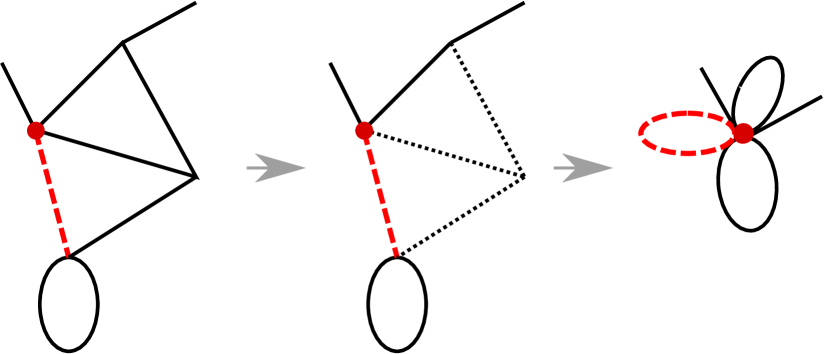
Figure 5.5. On the left, a graph $\Gamma$ with a choice of interior vertex $v$ and edge $e\in\mathcal{E}_{v}$. $v$ is marked in red and $e$ is dashed in red. On the middle, a choice of a spanning tree $T$ of $\Gamma\setminus\left\{e\right\}$. The edges of $T\setminus\mathcal{E}_{\partial\Gamma}$ are dotted. On the right, $\tilde{\Gamma}$, the graph obtained by contracting the dotted edges $T\setminus\mathcal{E}_{\partial\Gamma}$.

Consider a real solution to $\sum_{j=1}^{\left|\partial\Gamma\right|}t_{j}+2\sum_{j=\left|\partial\Gamma\right|+1}^{\beta+\left|\partial\Gamma\right|}t_{j}=0$ such that all $t_{j}$’s are non zero. Let $\tilde{\vec{\kappa}}$ be such that

$$\kappa_{j} =\begin{cases}\tan^{-1}\left(t_{j}\right)&\forall j\leq\left|\partial\Gamma\right|\\ 2\tan^{-1}\left(t_{j}\right)&\forall\left|\partial\Gamma\right|<j\leq\beta+\left|\partial\Gamma\right|\end{cases},\,\,\text{with}$$

$$\tan^{-1}: \mathbb{R}\setminus\left\{0\right\}\rightarrow\left(0,\frac{\pi}{2}\right)\cup\left(\frac{\pi}{2},\pi\right),$$

so by Lemma 5.23, $\tilde{\vec{\kappa}}\in\tilde{\Sigma}_{\mathcal{G}}$. Moreover, for any $u\in\partial\Gamma$ corresponding to the boundary vertex $v_{j}$,

$$\left|f_{\tilde{\vec{\kappa}}}\left(v_{j}\right)\right|=\left|\cos\left(\kappa_{j}\right)f_{\tilde{\vec{\kappa}}}\left(v_{0}\right)\right|\neq\left|f_{\tilde{\vec{\kappa}}}\left(v_{0}\right)\right|.$$

Let $\vec{\kappa}\in\mathbb{T}^{\mathcal{E}}$ given by the point $\tilde{\vec{\kappa}}$ above, as follows:

$$\vec{\kappa}{}_{e^{\prime}}=\begin{cases}\tilde{\kappa}_{e^{\prime}}&e^{\prime}\in\tilde{\Gamma}\\ 2\pi&e^{\prime}\in T_{\Gamma}\setminus\mathcal{E}_{\partial\Gamma}\end{cases},$$

Lemma C.4 states that if $e^{\prime\prime}$ is not a loop, $\Gamma_{\vec{\kappa}}$ is such that $\vec{\kappa}_{e^{\prime\prime}}=2\pi$, and $\Gamma_{\vec{\kappa}^{\prime\prime}}^{\prime\prime}$ is obtained by contracting $e^{\prime\prime}$ so that $\vec{\kappa}^{\prime\prime}$ and $\vec{\kappa}$ agree on all other edges, then

$$\dim Eig\left(\Gamma_{\vec{\kappa}},1\right)=\dim Eig\left(\Gamma^{\prime\prime}_{\vec{\kappa}^{\prime\prime}},1\right),$$

and if $\vec{\kappa}\in\Sigma^{reg}$, then the canonical eigenfunctions $f_{\vec{\kappa}}$ and $f_{\vec{\kappa}^{\prime\prime}}$ agree on all edges different than $e^{\prime\prime}$. Applying Lemma C.4 finitely many times, for each edge of $T_{\Gamma}\setminus\mathcal{E}_{\partial\Gamma}$, gives

$$\dim Eig\left(\Gamma_{\vec{\kappa}},1\right)=\dim Eig\left(\tilde{\Gamma}_{\tilde{\vec{\kappa}}},1\right).$$

Since $\tilde{\vec{\kappa}}\in\tilde{\Sigma}_{\mathcal{G}}$, then the above implies that $\vec{\kappa}\in\Sigma^{reg}$ and that for any $e^{\prime}\in\tilde{\Gamma}$ (including $e$) the restriction of the canonical eigenfunction $f_{\vec{\kappa}}|_{e^{\prime}}$ is equal to that of the $\tilde{\Gamma}$ canonical eigenfunction $f_{\tilde{\vec{\kappa}}}|_{e^{\prime}}$. In particular, since $\tilde{\vec{\kappa}}\in\tilde{\Sigma}_{\mathcal{G}}$, then

$$\left|\partial_{e}f_{\vec{\kappa}}\left(v\right)\right|=\left|\partial_{e}f_{\tilde{\vec{\kappa}}}\left(v_{0}\right)\right|\neq 0,$$

and for every $u\in\partial\Gamma$, corresponding to some $v_{j}$ vertex of the stower,

$$\left|f_{\vec{\kappa}}\left(u\right)\right|=\left|f_{\tilde{\vec{\kappa}}}\left(v_{j}\right)\right|\neq\left|f_{\tilde{\vec{\kappa}}}\left(v_{0}\right)\right|=\left|f_{\tilde{\vec{\kappa}}}\left(v\right)\right|.$$

∎

6. existence and symmetry of the nodal and Neumann statistics

In this section we construct the probabilistic setting needed in order to discuss the statistics of the nodal surplus and Neumann surplus. The results of this section appear in [8, 6].

Let $\Gamma_{\vec{l}}$ be a standard graph and let $\mathcal{G}$ be the index set of generic eigenfunctions, as in Definition 5.2. Let $\sigma,\omega:\mathcal{G}\rightarrow\mathbb{Z}$ be the nodal surplus and Neumann surplus sequences (see Definition 3.2). The discussion on nodal and Neumann counts is restricted, by definition, to the subset $\mathcal{G}$ and not to $\mathbb{N}$. The natural density (see Definition 4.27) is restricted accordingly:

Definition 6.1.

Let $\Gamma_{\vec{l}}$ be a standard graph and assume that $\mathcal{G}$ has positive density $d\left(\mathcal{G}\right)>0$. If $A\subset\mathcal{G}$ has density, we define its relative density as,

$$d_{\mathcal{G}}\left(A\right):=\lim_{N\rightarrow\infty}\frac{\left|A\left(N\right)\right|}{\left|\mathcal{G}\left(N\right)\right|}=\frac{d\left(A\right)}{d\left(\mathcal{G}\right)}.$$

Where $A\left(N\right)$ denotes $A\cap\left\{1,2,...N\right\}$ and same for $\mathcal{G}\left(N\right)$.

Remark 6.2.

The relative density $d_{\mathcal{G}}$ is not a measure on $\mathcal{G}$ in general (that is with the power set as $\sigma$-algebra), as it is not $\sigma$-additive. For example, $\forall j\in\mathcal{G}\,\,\,d_{\mathcal{G}}\left(\left\{j\right\}\right)=0$ but $d_{\mathcal{G}}\left(\sqcup_{j\in\mathcal{G}}\left\{j\right\}\right)=1$. Clearly, the image of $d_{\mathcal{G}}$ is in $\left[0,1\right]$ with $d_{\mathcal{G}}\left(\emptyset\right)=0$ and $d_{\mathcal{G}}\left(\mathcal{G}\right)=1$. Therefore, given a $\sigma$-algebra $\mathcal{F}$ on $\mathcal{G}$, $d_{\mathcal{G}}$ is a probability measure on $\left(\mathcal{G},\mathcal{F}\right)$ if and only if every set in $\mathcal{F}$ has density and $d_{\mathcal{G}}$ is $\sigma$-additive on $\mathcal{F}$.

We will now use the generic part of the secular manifold, $\Sigma_{\mathcal{G}}$ (see (5.11)), to define a $\sigma$-algebra on $\mathcal{G}$ on which $d_{\mathcal{G}}$ will be a probability measure.

Definition 6.3.

Let $\Gamma_{\vec{l}}$ be a standard graph with (square-root) eigenvalues $\left\{k_{n}\right\}_{n=0}^{\infty}$. Let $\Sigma_{\mathcal{G}}$ as defined in (5.11). For any connected component of $\Sigma_{\mathcal{G}}$, denoted by $\Sigma_{\mathcal{G},i}$, we define the index set $\mathcal{G}_{i}:=\left\{n\in\mathcal{G}\,\,:\,\,\left\{k_{n}\vec{l}\right\}\in\Sigma_{\mathcal{G},i}\right\}$. We define $\mathcal{F}_{\mathcal{G}}$ to be the $\sigma$-algebra of $\mathcal{G}$ generated by all $\mathcal{G}_{i}$’s.

Remark 6.4.

As the $\mathcal{G}_{i}$’s are disjoint, then they are the atoms of $\mathcal{F}_{\mathcal{G}}$, and any set $A\in\mathcal{F}_{\mathcal{G}}$ is a (countable) disjoint union of atoms.

The main theorem of this section, combines Theorem 2.1 of [8] and Theorem 3.5 of [6]:

Theorem 6.5.

Let $\Gamma_{\vec{l}}$ be a standard graph with $\vec{l}$ rationally independent. Then,

1. The relative density, $d_{\mathcal{G}}$, is a probability measure on $\left(\mathcal{G},\mathcal{F}_{\mathcal{G}}\right)$ and we denote the probability space by the triplet $\left(\mathcal{G},\mathcal{F}_{\mathcal{G}},d_{\mathcal{G}}\right)$. Moreover, every atom $\mathcal{G}_{i}$ has positive probability given by,

   $$d_{\mathcal{G}}\left(\mathcal{G}_{i}\right)=\frac{\mu_{\vec{l}}\left(\Sigma_{\mathcal{G},i}\right)}{\mu_{\vec{l}}\left(\Sigma_{\mathcal{G}}\right)}>0.$$

2. Both $\sigma$ and $\omega$ are finite random variables on $\left(\mathcal{G},\mathcal{F}_{\mathcal{G}},d_{\mathcal{G}}\right)$.
   In particular, for any possible value $j$, the following limits exist and define the probabilities of the events $\sigma^{-1}\left(j\right):=\left\{\sigma=j\right\}$ or $\omega^{-1}\left(j\right):=\left\{\omega=j\right\}$:

   (6.1) $$P\left(\sigma=j\right) :=d_{\mathcal{G}}\left(\sigma^{-1}\left(j\right)\right)=\lim_{N\rightarrow\infty}\frac{\left|\left\{n\in\mathcal{G}\left(N\right)\,\,:\,\,\sigma_{n}=j\right\}\right|}{\left|\mathcal{G}\left(N\right)\right|}$$

   (6.2) $$P\left(\omega=j\right) :=d_{\mathcal{G}}\left(\omega^{-1}\left(j\right)\right)=\lim_{N\rightarrow\infty}\frac{\left|\left\{n\in\mathcal{G}\left(N\right)\,\,:\,\,\omega_{n}=j\right\}\right|}{\left|\mathcal{G}\left(N\right)\right|}.$$

3. The random variables $\sigma$ and $\omega$ are symmetric around $\frac{\beta}{2}$ and $\frac{\beta-\left|\partial\Gamma\right|}{2}$ simultaneously. That is, the joint probability of the event

   $$\left\{\sigma=i\,\wedge\,\omega=j\right\}:=\sigma^{-1}\left(i\right)\cap\omega^{-1}\left(j\right),$$

   which is given by

   (6.3) $$P\left(\sigma=j\,\,\wedge\,\,\omega=i\right):=d_{\mathcal{G}}\left(\sigma^{-1}\left(j\right)\cap\omega^{-1}\left(i\right)\right),$$

   satisfies the symmetry:

   (6.4) $$P\left(\sigma=j\,\,\wedge\,\,\omega=i\right) =P\left(\sigma=\beta-j\,\,\wedge\,\,\omega=\beta-\left|\partial\Gamma\right|-i\right).$$

4. Every value of the pair $\left(\sigma,\omega\right)$ which is attained once, appears infinitely often with positive density. Namely, if $\sigma\left(n\right)=i$ and $\omega\left(n\right)=j$ for some $n\in\mathcal{G}$, then $P\left(\sigma=j\,\,\wedge\,\,\omega=i\right)>0$.

Before proving this theorem we will first state a corollary of this theorem. An inverse result, showing how $\beta$ and $\partial\Gamma$ can be obtained from the nodal and Neumann averages:

Corollary 6.6.

Let $\Gamma_{\vec{l}}$ be a standard graph with $\vec{l}$ rationally independent and first Betti number $\beta$. Then,

$$\mathbb{E}\left(\sigma\right)=\lim_{N\rightarrow\infty}\frac{1}{\left|\mathcal{G}(N)\right|}\sum_{n\in\mathcal{G}(N)}\sigma(n) =\frac{\beta}{2},\,\,\text{and}$$

$$\mathbb{E}\left(\omega\right)=\lim_{N\rightarrow\infty}\frac{1}{\left|\mathcal{G}(N)\right|}\sum_{n\in\mathcal{G}(N)}\omega(n) =\frac{\beta-\left|\partial\Gamma\right|}{2}.$$

Remark 6.7.

If Conjecture 3.6 is true, as discussed in Remark 3.7, then $\sigma$ and $\omega$ are not independent. Such lack of independence can be spotted in Figure 6.1, where the $\left(\sigma,\omega\right)$ statistics of a random regular graph is provided. The support of the joint distribution of $\left(\sigma,\omega\right)$ is not rectangular which implies that they are not independent.

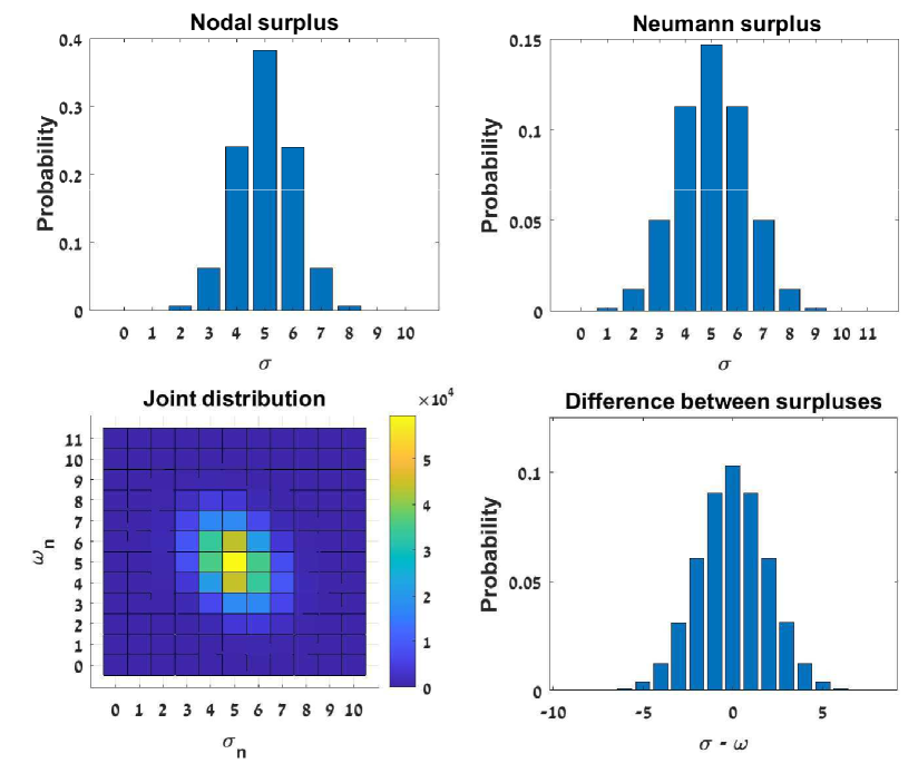
Figure 6.1. Nodal and Neumann statistics for the complete graph of 6 vertices using $10^{6}$ eigenfunctions. On the upper left, the nodal surplus distribution. On the upper right, the Neumann surplus distribution. On the bottom right, the distribution of the difference $\sigma-\omega$. On the bottom left, a joint distribution of $\left(\sigma,\omega\right)$.

The proof of Theorem 2.1 in [8] relied on a result called the nodal magnetic theorem [39] that was discussed in the introduction and will be presented in Section 8. The result of Theorem 3.5 in [6] relied on Theorem 2.1 in [8], and therefore on the nodal magnetic theorem. We will now present a proof of both, which does not rely on the nodal magnetic theorem.

Definition 6.8.

We define the spectral counting function of the standard graph $\Gamma_{\vec{l}}$ as follows:

$$N\left(\Gamma_{\vec{l}},k\right):=\left|\left\{0<\lambda\leq k^{2}\,\,:\,\,\lambda\,\,\text{is and eigenvalue of}\,\,\Gamma_{\vec{l}}\right\}\right|,$$

where the counting includes multiplicity. If $k_{n}$ is a simple eigenvalue of $\Gamma_{\vec{l}}$, then its spectral position is $n$ and is equal to $N\left(\Gamma_{\vec{l}},k_{n}\right)$. Given $\vec{\kappa}\in\Sigma^{reg}$, we define the spectral position $n\left(\vec{\kappa}\right)$, as

(6.5) $$n\left(\vec{\kappa}\right):=N\left(\Gamma_{\vec{\kappa}},1\right).$$

See Figure 6.2 for example of a secular manifold colored according to the spectral position. One can see in Figure 6.2 that a line in $(0,2\pi)^{\mathcal{E}}$ connecting the origin to a point on the $n=2$ layer will hit the $n=1$ layer once. In the same way, such a line from the origin to a point with $n=3$ will first cross the $n=1$ and $n=2$ layers.

Figure 6.2. On the right, a ‘3-mandarin’ graph $\Gamma$. On the left, the secular manifold $\Sigma$, colored according to the spectral position $n$. The first layer, $n=1$, in green. The second layer, $n=2$, in yellow. The third layer, $n=3$, in red.

The torus $\mathbb{T}^{n}$ may be embedded into $\left(0,2\pi\right]^{n}$ or into $\left[0,2\pi\right)^{n}$ and the $l_{1}$ norm of a point in $\mathbb{T}^{n}$ will depend on the choice of embedding. To avoid obscurity, as we will use both of these embeddings, we define the following.

Definition 6.9.

Define the two embeddings $r_{0}:\mathbb{T}\rightarrow\left[0,2\pi\right)$ and $r_{2\pi}:\mathbb{T}\rightarrow\left(0,2\pi\right]$ and extend them to $\mathbb{T}^{\mathcal{E}}$ by

$$r_{0}\left(\vec{\kappa}\right):=\sum_{e\in\mathcal{E}}r_{0}\left(\kappa_{e}\right),\,\,r_{2\pi}\left(\vec{\kappa}\right):=\sum_{e\in\mathcal{E}}r_{2\pi}\left(\kappa_{e}\right).$$

Remark 6.10.

In particular, the total length of the standard graph $\Gamma_{\vec{\kappa}}$ is $r_{2\pi}\left(\vec{\kappa}\right)$.

6.1. The difference $N\left(\Gamma_{\vec{l}},k\right)-\frac{L}{\pi}k$.

Kottos and Smilansky derived the quantum graphs trace formula in [83, 84] as the derivative of the trace formula of the spectral counting function $k\mapsto N\left(\Gamma_{\vec{l}},k\right)$. They showed that for a standard graph $\Gamma_{\vec{l}}$ of total length $L=\sum_{e\in\mathcal{E}}l_{e}$, $N\left(\Gamma_{\vec{l}},k\right)$ is given in terms of the Weyl term $\frac{L}{\pi}k$ and a formal sum on the traces of the unitary evolution matrix $U_{\left\{k\vec{l}\right\}}$:

(6.6) $$N\left(\Gamma_{\vec{l}},k\right)=\frac{1}{2}+\frac{L}{\pi}k+\frac{1}{\pi}\Im\left[\sum_{n=1}^{\infty}\frac{1}{n}\mathrm{trace}\left(U_{\left\{k\vec{l}\right\}}^{n}\right)\right].$$

The formal sum $\frac{1}{\pi}\Im\left[\sum_{n=1}^{\infty}\frac{1}{n}\mathrm{trace}\left(U_{\left\{k\vec{l}\right\}}^{n}\right)\right]$ should be evaluated at $k+i\epsilon$ with $\epsilon>0$, for which the sum converges, and then take the limit $\epsilon\rightarrow+0$. This sum is usually called the oscillatory part. For convenience, we will include the constant $\frac{1}{2}$ in our definition of the oscillatory part:

(6.7) $$N_{osc}\left(\Gamma_{\vec{l}},k\right):=N\left(\Gamma_{\vec{l}},k\right)-\frac{L}{\pi}k.$$

Obviously, the summands of the formal sum depend only on $\vec{\kappa}=\left\{k\vec{l}\right\}$ and so $N_{osc}\left(\Gamma_{\vec{l}},k_{n}\right)$ for simple $k_{n}$ should be a function on $\Sigma^{reg}$. We will present a proof that $N_{osc}\left(\Gamma_{\vec{l}},k_{n}\right)$ is a function of $\left\{k_{n}\vec{l}\right\}$ on $\Sigma^{reg}$, avoiding the formal sum, by following the method of [84] which is also presented in Section 5.1 in [71].

Lemma 6.11.

Let $\Gamma_{\vec{l}}$ be a standard graph of total length $L$ and let $k^{2}$ be a simple eigenvalue. Denote $\vec{\kappa}=\left\{k\vec{l}\right\}$, then

(6.8) $$N_{osc}\left(\Gamma_{\vec{l}},k\right)=n\left(\vec{\kappa}\right)-\frac{r_{2\pi}\left(\vec{\kappa}\right)}{\pi}.$$

Moreover, the function $n\left(\vec{\kappa}\right)-\frac{r_{2\pi}\left(\vec{\kappa}\right)}{\pi}$ is continuous on $\Sigma^{reg}$ and is symmetric around $-\frac{\beta}{2}$ with respect to the inversion $\mathcal{I}\left(\vec{\kappa}\right)=\left\{-\vec{\kappa}\right\}$. Namely

$$n\left(\mathcal{I}\left(\vec{\kappa}\right)\right)-\frac{r_{2\pi}\left(\mathcal{I}\left(\vec{\kappa}\right)\right)}{\pi}=-\beta-\left(n\left(\vec{\kappa}\right)-\frac{r_{2\pi}\left(\vec{\kappa}\right)}{\pi}\right).$$

Remark 6.12.

We will use the inversion notation $\mathcal{I}$ also for the entries of $\vec{\kappa}$, namely $\mathcal{I}\left(\kappa_{e}\right):=\left\{-\kappa_{e}\right\}$, and for the diagonal exponent matrix $e^{i\hat{\kappa}}$ such that $e^{i\mathcal{I}\hat{\kappa}}=e^{-i\hat{\kappa}}$.

Proof.

Let $U_{\vec{\kappa}}=e^{i\hat{\kappa}}S$ be the unitary evolution matrix as defined in (4.11), and consider the one parameter family $t\mapsto U_{\left\{t\vec{l}\right\}}$ for $t>0$. Let $\left\{e^{i\theta_{j}}\right\}_{j=1}^{2E}$ be a continuous choice of eigenvalues of $U_{\left\{t\vec{l}\right\}}$ with orthonormal eigenvectors $\left\{a_{j}\right\}_{j=1}^{2E}$. All $\left\{e^{i\theta_{j}}\right\}_{j=1}^{2E}$ and $\left\{a_{j}\right\}_{j=1}^{2E}$ depend smoothly on $t$ as long as the $\left\{e^{i\theta_{j}}\right\}_{j=1}^{2E}$ eigenvalues are simple, and are continuous in $t$ when there are non-simple eigenvalues. For readability we do not write the $t$ dependence explicitly. Denote the tuple of angles by $\vec{\theta}\in\mathbb{T}^{2E}$ with derivatives $\frac{d}{dt}\vec{\theta}\in\mathbb{R}^{2E}$. It is not hard to deduce from (4.11) that $\frac{d}{dt}U_{t\vec{l}}=i\hat{L}U_{t\vec{l}}$ where $\hat{L}$ is diagonal with entries $\left(\hat{L}\right)_{e,e}=\left(\hat{L}\right)_{\hat{e},\hat{e}}=l_{e}$. We calculate $\frac{d}{dt}\theta_{j}$ by taking derivative of the relation $\left(e^{i\theta_{j}}-U_{t\vec{l}}\right)a_{j}=0$, which gives

$$\left(i\frac{d}{dt}\theta_{j}e^{i\theta_{j}}-i\hat{L}U_{t\vec{l}}\right)a_{j}+\left(e^{i\theta_{j}}-U_{t\vec{l}}\right)\frac{d}{dt}a_{j}=0.$$

Taking the inner product of the above equation with $a_{j}$ (where $\left\langle*,*\right\rangle$ denote the standard $\mathbb{C}^{\vec{\mathcal{E}}}$ inner product) gives $\left\langle a_{j},\left(e^{i\theta_{j}}-U_{t\vec{l}}\right)\frac{d}{dt}a_{j}\right\rangle=0$ for the right summand and therefore

$$\left\langle a_{j},i\frac{d}{dt}\theta_{j}e^{i\theta_{j}}a_{j}\right\rangle-\left\langle a_{j},i\hat{L}U_{t\vec{l}}a_{j}\right\rangle=ie^{i\theta}\left(\frac{d}{dt}\theta_{j}-\left\langle a_{j},\hat{L}a_{j}\right\rangle\right)=0.$$

We conclude that whenever it is defined (i.e $e^{i\theta_{j}}$ is simple), $\frac{d}{dt}\theta_{j}$ is given by:

$$\frac{d}{dt}\theta_{j}=\left\langle a_{j},\hat{L}a_{j}\right\rangle=\sum_{e\in\mathcal{E}}l_{e}\left(\left|\left(a_{j}\right)_{e}\right|^{2}+\left|\left(a_{j}\right)_{\hat{e}}\right|^{2}\right)>0.$$

In particular, if we denote $L_{min}=\min_{e\in\mathcal{E}}\left\{l_{e}\right\}$ and $L_{max}=\max_{e\in\mathcal{E}}\left\{l_{e}\right\}$, then the normalization

$$\left\|a_{j}\right\|^{2}=\sum_{e\in\mathcal{E}}\left|\left(a_{j}\right)_{e}\right|^{2}+\left|\left(a_{j}\right)_{\hat{e}}\right|^{2}=1,$$

implies that

$$L_{min}\leq\sum_{e\in\mathcal{E}}l_{e}\left(\left|\left(a_{j}\right)_{e}\right|^{2}+\left|\left(a_{j}\right)_{\hat{e}}\right|^{2}\right)\leq L_{max}.$$

Therefore, $\frac{d}{dt}\theta_{j}$ is strictly positive, and is bounded by:

$$L_{min}\leq\frac{d}{dt}\theta_{j}\leq L_{max}.$$

Moreover, as $\left\{a_{j}\right\}_{j=1}^{2E}$ is an orthonormal basis, then

(6.9) $$\sum_{j=1}^{2E}\frac{d}{dt}\theta_{j}=\sum_{j=1}^{2E}\left\langle a_{j},\hat{L}a_{j}\right\rangle=\mathrm{trace}\left(\hat{L}\right)=2L.$$

If we now consider a simple eigenvalue $k^{2}$, then $N\left(\Gamma_{\vec{l}},k\right)$ can be calculated by:

(6.10) $$N\left(\Gamma_{\vec{l}},k\right) =\sum_{j=1}^{2E}\left|\left\{0<t\leq k\,\,:\,\,e^{i\theta_{j}}|_{t}=1\right\}\right|.$$

Since $\frac{d}{dt}\theta_{j}>0$, then each summand $\left|\left\{0<t\leq k\,\,:\,\,e^{i\theta_{j}}|_{t}=1\right\}\right|$ is given by integrating $\frac{d}{dt}\theta_{j}$ as follows.

$$\left|\left\{0<t\leq k\,\,:\,\,e^{i\theta_{j}}|_{t}=1\right\}\right|=\frac{r_{0}\left(\theta_{j}|_{0}\right)}{2\pi}+\frac{1}{2\pi}\int_{0}^{k}\frac{d}{dt}\theta_{j}dt-\frac{r_{0}\left(\theta_{j}|_{k}\right)}{2\pi},$$

and summing over $j$, using $\sum_{j=1}^{2E}\frac{1}{2\pi}\int_{0}^{k}\frac{d}{dt}\theta_{j}dt=\frac{1}{2\pi}\int_{0}^{k}2Ldt=\frac{L}{\pi}k$, gives:

(6.11) $$N\left(\Gamma_{\vec{l}},k\right) =\frac{L}{\pi}k+\sum_{j=1}^{2E}\frac{r_{0}\left(\theta_{j}|_{0}\right)}{2\pi}-\frac{r_{0}\left(\theta_{j}|_{k}\right)}{2\pi},\,\,\text{and so }$$

(6.12) $$N_{osc}\left(\Gamma_{\vec{l}},k\right) =\frac{r_{0}\left(\vec{\theta}|_{0}\right)}{2\pi}-\frac{r_{0}\left(\vec{\theta}|_{k}\right)}{2\pi}.$$

Observe that $U_{t\vec{l}}$ at $t=0$ is simply $S$, the real orthogonal scattering matrix in Definition 4.13, and therefore its non-real eigenvalues come in conjugated pairs, so

$$\frac{r_{0}\left(\vec{\theta}|_{0}\right)}{2\pi}=\frac{1}{2}\left|\left\{j\,\,:\,\,e^{i\theta_{j}}|_{0}\neq 1\right\}\right|=E-\frac{1}{2}\dim\ker\left(1-S\right).$$

In [88] (a correction to [87]) it was shown that $\dim\ker\left(1-S\right)=E-V+2$, hence $\frac{r_{0}\left(\vec{\theta}|_{0}\right)}{2\pi}=\frac{E+V}{2}-1$. We may conclude that,

(6.13) $$N_{osc}\left(\Gamma_{\vec{l}},k\right)=\frac{E+V}{2}-1-\frac{r_{0}\left(\vec{\theta}|_{k}\right)}{2\pi}.$$

As $U_{t\vec{l}}$ for $t=k$ is equal to $U_{\vec{\kappa}}$, then $\frac{r_{0}\left(\vec{\theta}|_{k}\right)}{2\pi}$ is a function of $\vec{\kappa}$, and therefore $N_{osc}\left(\Gamma_{\vec{l}},k\right)$ is a function of $\vec{\kappa}$, and so $N_{osc}\left(\Gamma_{\vec{l}},k\right)=N_{osc}\left(\Gamma_{\vec{\kappa}},1\right)$ for any simple eigenvalue $k>0$. As the graph $\Gamma_{\vec{\kappa}}$ is of total length $r_{2\pi}\left(\vec{\kappa}\right)$, we may conclude that

(6.14) $$N_{osc}\left(\Gamma_{\vec{l}},k\right)=n\left(\vec{\kappa}\right)-\frac{r_{2\pi}\left(\vec{\kappa}\right)}{\pi}.$$

In order to prove that $n\left(\vec{\kappa}\right)-\frac{r_{2\pi}\left(\vec{\kappa}\right)}{\pi}$ is continuous over $\Sigma^{reg}$, we can use (6.13), denoting the angles of the eigenvalues of $U_{\vec{\kappa}}$ by $\vec{\theta}|_{\vec{\kappa}}$:

(6.15) $$\forall\vec{\kappa}\in\Sigma^{reg}\,\,\,\,n\left(\vec{\kappa}\right)-\frac{r_{2\pi}\left(\vec{\kappa}\right)}{\pi}=\frac{E+V}{2}-1-\frac{r_{0}\left(\vec{\theta}|_{\vec{\kappa}}\right)}{2\pi}.$$

So we need to prove that $r_{0}\left(\vec{\theta}|_{\vec{\kappa}}\right)$ is continuous on $\Sigma^{reg}$. Since $U_{\vec{\kappa}}$ is continuous in $\vec{\kappa}$, then so does its eigenvalues. Therefore $\vec{\theta}|_{\vec{\kappa}}:\Sigma^{reg}\rightarrow\mathbb{T}^{2E}$ is continuous. Let $\vec{\kappa}\in\Sigma^{reg}$ and number the eigenvalues such that $e^{i\theta_{1}}|_{\vec{\kappa}}=1$ and hence $e^{i\theta_{j}}|_{\vec{\kappa}}\neq 1$ for all $j>1$ (as $\dim\ker\left(1-U_{\vec{\kappa}}\right)$). By the continuity of the eigenvalues, there is a neighborhood of $\vec{\kappa}$, $O\subset\Sigma^{reg}$, such that $\forall\vec{\kappa}^{\prime}\in O$, $e^{i\theta_{1}}|_{\vec{\kappa}^{\prime}}=1$ and $e^{i\theta_{j}}|_{\vec{\kappa}^{\prime}}\neq 1$ for all $j>1$. In particular, $r_{0}\left(\vec{\theta}|_{\vec{\kappa}^{\prime}}\right)=0+\sum_{j>1}r_{0}\left(\theta_{j}|_{\vec{\kappa}^{\prime}}\right)$ in $O$, and each $r_{0}\left(\theta_{j}|_{\vec{\kappa}^{\prime}}\right)$ is continuous since $e^{i\theta_{j}}|_{\vec{\kappa}^{\prime}}\neq 1$. It follows that $r_{0}\left(\vec{\theta}|_{\vec{\kappa}^{\prime}}\right)$ is continuous in $O$ and therefore on $\Sigma^{reg}$ as $\vec{\kappa}$ was arbitrary. This proves that $n\left(\vec{\kappa}\right)-\frac{r_{2\pi}\left(\vec{\theta}|_{\vec{\kappa}}\right)}{2\pi}$ is continuous on $\Sigma^{reg}$ as needed.

To prove the symmetry recall that

$$U_{\mathcal{I}\left(\vec{\kappa}\right)}=e^{i\mathcal{I}\left(\hat{\kappa}\right)}S=e^{-i\hat{\kappa}}S=\overline{U_{\vec{\kappa}}},$$

and so for any $\vec{\kappa}\in\Sigma^{reg}$,

(6.16) $$\frac{r_{0}\left(\vec{\theta}|_{\mathcal{I}\left(\vec{\kappa}\right)}\right)}{2\pi}=\frac{1}{2\pi}\sum_{j=1}^{2E}\begin{cases}0&e^{i\theta_{j}}=1\\ 2\pi-r_{0}\left(\theta_{j}|_{\vec{\kappa}^{\prime}}\right)&e^{i\theta_{j}}\neq 1\end{cases}=2E-1-\frac{r_{0}\left(\vec{\theta}|_{\vec{\kappa}}\right)}{2\pi}.$$

Using (6.15) and $\beta=E-V+1$, we get the needed result:

$$n\left(\mathcal{I}\left(\vec{\kappa}\right)\right)-\frac{r_{2\pi}\left(\mathcal{I}\left(\vec{\kappa}\right)\right)}{\pi} =\frac{E+V}{2}-1-\left(2E-1-\frac{r_{0}\left(\vec{\theta}|_{\vec{\kappa}}\right)}{2\pi}\right)$$

$$= -E+V-1-\left(\frac{E+V}{2}-1-\frac{r_{0}\left(\vec{\theta}|_{\vec{\kappa}}\right)}{2\pi}\right)$$

$$= -\beta-\left(n\left(\vec{\kappa}\right)-\frac{r_{2\pi}\left(\vec{\kappa}\right)}{\pi}\right).$$

∎

6.2. The differences $\phi\left(f\right)-\frac{L}{\pi}k$ and $\mu\left(f\right)-\frac{L}{\pi}k$

Given a standard graph $\Gamma_{\vec{l}}$ with a generic eigenfunction $f$ of eigenvalue $k^{2}$, the nodal surplus and Neumann surplus of $f$ are given by $\phi\left(f\right)-N\left(\Gamma_{\vec{l}},k\right)$ and $\mu\left(f\right)-N\left(\Gamma_{\vec{l}},k\right)$ as in Definition 3.2. Since $N\left(\Gamma_{\vec{l}},k\right)-\frac{L}{\pi}k$ was shown to be a continuous function on $\Sigma^{reg}$, we will be able to show that the nodal and Neumann surplus are continuous functions on $\Sigma_{\mathcal{G}}$ by proving that the differences $\phi\left(f\right)-\frac{L}{\pi}k$ and $\mu\left(f\right)-\frac{L}{\pi}k$ are continuous functions on $\Sigma_{\mathcal{G}}$.

Lemma 6.13.

Let $\Gamma_{\vec{l}}$ be a standard graph of total length $L$ and let $f$ be a generic eigenfunction of eigenvalue $k^{2}$. Denote $\vec{\kappa}=\left\{k\vec{l}\right\}\in\Sigma_{\mathcal{G}}$ and let $f_{\vec{\kappa}}$ be the associated canonical eigenfunction. Then,

(6.17) $$\phi\left(f\right)-\frac{L}{\pi}k =\phi\left(f_{\vec{\kappa}}\right)-\frac{r_{2\pi}\left(\vec{\kappa}\right)}{\pi}$$

(6.18) $$\mu\left(f\right)-\frac{L}{\pi}k =\mu\left(f_{\vec{\kappa}}\right)-\frac{r_{2\pi}\left(\vec{\kappa}\right)}{\pi}.$$

Moreover, both $\phi\left(f_{\vec{\kappa}}\right)-\frac{r_{2\pi}\left(\vec{\kappa}\right)}{\pi}$ and $\mu\left(f_{\vec{\kappa}}\right)-\frac{r_{2\pi}\left(\vec{\kappa}\right)}{\pi}$ are continuous on $\Sigma^{\mathcal{G}}$, and satisfy the following symmetry:

(6.19) $$\phi\left(f_{\mathcal{I}\left(\vec{\kappa}\right)}\right)-\frac{r_{2\pi}\left(\mathcal{I}\left(\vec{\kappa}\right)\right)}{\pi} =-\left(\phi\left(f_{\vec{\kappa}}\right)-\frac{r_{2\pi}\left(\vec{\kappa}\right)}{\pi}\right)$$

(6.20) $$\mu\left(f_{\mathcal{I}\left(\vec{\kappa}\right)}\right)-\frac{r_{2\pi}\left(\mathcal{I}\left(\vec{\kappa}\right)\right)}{\pi} =-\left(\mu\left(f_{\vec{\kappa}}\right)-\frac{r_{2\pi}\left(\vec{\kappa}\right)}{\pi}\right)-\left|\partial\Gamma\right|.$$

Proof.

Denote the nodal and Neumann counts of the restriction $f|_{e}$ for an edge $e$ by $\phi\left(f|_{e}\right)$ and $\mu\left(f|_{e}\right)$. Since $f|_{e}\not\equiv 0$ as it is generic, the by Definition 2.16, it is periodic on $e$ with period $\frac{2\pi}{k}$ and in every interval $\left(a,b\right]$ of length $\frac{\pi}{k}$ it gets exactly one nodal and one Neumann point. Therefore, both $\phi\left(f|_{e}\right)$ and $\mu\left(f|_{e}\right)$ are given by twice the number of periods, $2\left\lfloor\frac{kl_{e}}{2\pi}\right\rfloor$, plus a correction of either $0,1$ or $2$. In particular if the reminder (in half periods) $\frac{kl_{e}}{\pi}-2\left\lfloor\frac{kl_{e}}{2\pi}\right\rfloor\leq 1$ then the corrections are either $0$ or $1$, and if $\frac{kl_{e}}{\pi}-2\left\lfloor\frac{kl_{e}}{2\pi}\right\rfloor\geq 1$ then they are either $1$ or $2$.

Let $v,u$ be the vertices of $e$. To determine $\phi\left(f|_{e}\right)-2\left\lfloor\frac{kl_{e}}{2\pi}\right\rfloor$, notice that $f\left(v\right)f\left(u\right)<0$ implies $\phi\left(f|_{e}\right)$ is odd ,in which case $\phi\left(f|_{e}\right)=2\left\lfloor\frac{kl_{e}}{2\pi}\right\rfloor+1$. Otherwise $f\left(v\right)f\left(u\right)>0$ (by genericity) and therefore $\phi\left(f|_{e}\right)$ is even, so $\phi\left(f|_{e}\right)-2\left\lfloor\frac{kl_{e}}{2\pi}\right\rfloor$ is either $0$ or $2$. In such case

$$\phi\left(f|_{e}\right)=\begin{cases}2\left\lfloor\frac{kl_{e}}{2\pi}\right\rfloor&kl_{e}-2\pi\left\lfloor\frac{kl_{e}}{2\pi}\right\rfloor\in\left[0,\pi\right)\\ 2\left\lfloor\frac{kl_{e}}{2\pi}\right\rfloor+2&kl_{e}-2\pi\left\lfloor\frac{kl_{e}}{2\pi}\right\rfloor\in\left(\pi,2\pi\right)\end{cases}.$$

We excluded $kl_{e}-2\pi\left\lfloor\frac{kl_{e}}{2\pi}\right\rfloor=\pi$ as it implies $f\left(v\right)f\left(u\right)<0$. Using $\vec{\kappa}=\left\{k\vec{l}\right\}$ we can write $kl_{e}-2\pi\left\lfloor\frac{kl_{e}}{2\pi}\right\rfloor=r_{0}\left(\kappa_{e}\right)$, and given the canonical eigenfunction $f_{\vec{\kappa}}$ and Lemma 4.11 we get $f\left(v\right)f\left(u\right)=f_{\vec{\kappa}}\left(v\right)f_{\vec{\kappa}}\left(u\right)$. Therefore, the difference $\phi\left(f|_{e}\right)-\frac{kl_{e}}{\pi}$ is a $\vec{\kappa}$ dependent function:

(6.21) $$\phi\left(f|_{e}\right)-\frac{kl_{e}}{\pi} =\begin{cases}-\frac{r_{0}\left(\kappa_{e}\right)}{\pi}&f_{\vec{\kappa}}\left(v\right)f_{\vec{\kappa}}\left(u\right)>0\,\,and\,\,r_{0}\left(\kappa_{e}\right)\in\left[0,\pi\right)\\ 1-\frac{r_{0}\left(\kappa_{e}\right)}{\pi}&f_{\vec{\kappa}}\left(v\right)f_{\vec{\kappa}}\left(u\right)<0\\ 2-\frac{r_{0}\left(\kappa_{e}\right)}{\pi}&f_{\vec{\kappa}}\left(v\right)f_{\vec{\kappa}}\left(u\right)>0\,\,and\,\,r_{0}\left(\kappa_{e}\right)\in\left(\pi,2\pi\right)\end{cases}.$$

In particular,

(6.22) $$\phi\left(f|_{e}\right)-\frac{kl_{e}}{\pi}=\phi\left(f_{\vec{\kappa}}|_{e}\right)-\frac{r_{2\pi}\left(\kappa_{e}\right)}{\pi}.$$

Let $M$ be a connected component of $\Sigma_{\mathcal{G}}$. According to Lemma 4.25, $f_{\vec{\kappa}}\left(v\right)f_{\vec{\kappa}}\left(u\right)$ is a real, continuous and non vanishing function on $M$ so it has a fixed sign. The vertex values, as seen from Definition 2.16, satisfy $f_{\vec{\kappa}}\left(v\right)=f_{\vec{\kappa}}\left(u\right)$ in case that $e^{i\kappa_{e}}=1$ and $f_{\vec{\kappa}}\left(v\right)=-f_{\vec{\kappa}}\left(u\right)$ if $e^{i\kappa_{e}}=-1$. It follows that if $f_{\vec{\kappa}}\left(v\right)f_{\vec{\kappa}}\left(u\right)<0$ on $M$, then $e^{i\kappa_{e}}\neq 1$ on $M$ and therefore $\frac{r_{0}\left(\kappa_{e}\right)}{\pi}$ is continuous on $M$ and so does $\phi\left(f_{\vec{\kappa}}|_{e}\right)-\frac{r_{2\pi}\left(\kappa_{e}\right)}{\pi}=1-\frac{r_{0}\left(\kappa_{e}\right)}{\pi}$. If $f_{\vec{\kappa}}\left(v\right)f_{\vec{\kappa}}\left(u\right)>0$ on $M$, then $e^{i\kappa_{e}}\neq-1$ and as $-\frac{r_{0}\left(\kappa_{e}\right)}{\pi}$ and $2-\frac{r_{0}\left(\kappa_{e}\right)}{\pi}$ agree when $e^{i\kappa_{e}}=1$ so the function

$$\phi\left(f_{\vec{\kappa}}|_{e}\right)-\frac{r_{2\pi}\left(\kappa_{e}\right)}{\pi}=\begin{cases}-\frac{r_{0}\left(\kappa_{e}\right)}{\pi}&r_{0}\left(\kappa_{e}\right)\in\left[0,\pi\right)\\ 2-\frac{r_{0}\left(\kappa_{e}\right)}{\pi}&r_{0}\left(\kappa_{e}\right)\in\left(\pi,2\pi\right)\end{cases}$$

is continuous on $M$. To prove the symmetry, consider the point $\mathcal{I}\left(\vec{\kappa}\right)$ and notice that

$$r_{0}\left(\mathcal{I}\left(\kappa_{e}\right)\right)=\begin{cases}2\pi-r_{0}\left(\kappa_{e}\right)&r_{0}\left(\kappa_{e}\right)\neq 0\\ 0&r_{0}\left(\kappa_{e}\right)=0\end{cases}$$

and $f_{\mathcal{I}\left(\vec{\kappa}\right)}\left(v\right)f_{\mathcal{I}\left(\vec{\kappa}\right)}\left(u\right)=f_{\vec{\kappa}}\left(v\right)f_{\vec{\kappa}}\left(u\right)$ according to Lemma 4.25. Substituting the latter into (6.21) gives,

$$\phi\left(f_{\mathcal{I}\left(\vec{\kappa}\right)}|_{e}\right)-\frac{r_{2\pi}\left(\mathcal{I}\left(\kappa_{e}\right)\right)}{\pi} =\begin{cases}0&r_{0}\left(\kappa_{e}\right)=0\\ \frac{r_{0}\left(\kappa_{e}\right)}{\pi}-2&f_{\vec{\kappa}}\left(v\right)f_{\vec{\kappa}}\left(u\right)>0\,\,and\,\,r_{0}\left(\mathcal{I}\left(\kappa_{e}\right)\right)\in\left(0,\pi\right)\\ \frac{r_{0}\left(\kappa_{e}\right)}{\pi}-1&f_{\vec{\kappa}}\left(v\right)f_{\vec{\kappa}}\left(u\right)<0\\ \frac{r_{0}\left(\kappa_{e}\right)}{\pi}&f_{\vec{\kappa}}\left(v\right)f_{\vec{\kappa}}\left(u\right)>0\,\,and\,\,r_{0}\left(\mathcal{I}\left(\kappa_{e}\right)\right)\in\left(\pi,2\pi\right)\end{cases}$$

$$= -\left(\phi\left(f_{\vec{\kappa}}|_{e}\right)-\frac{r_{2\pi}\left(\kappa_{e}\right)}{\pi}\right).$$

We may now sum over all edges to conclude that

$$\phi\left(f\right)-\frac{L}{\pi}k=\phi\left(f_{\vec{\kappa}}\right)-\frac{r_{2\pi}\left(\vec{\kappa}\right)}{\pi}.$$

It is continuous on $\Sigma_{\mathcal{G}}$ and satisfy

$$\phi\left(f_{\mathcal{I}\left(\vec{\kappa}\right)}\right)-\frac{r_{2\pi}\left(\mathcal{I}\left(\vec{\kappa}\right)\right)}{\pi}=-\left(\phi\left(f_{\vec{\kappa}}\right)-\frac{r_{2\pi}\left(\vec{\kappa}\right)}{\pi}\right).$$

The analysis of $\mu\left(f\right)-\frac{L}{\pi}k$ is in the same spirit. To determine $\mu\left(f|_{e}\right)-2\left\lfloor\frac{kl_{e}}{2\pi}\right\rfloor$ we consider first the case where both $v$ and $u$ are internal vertices. In such case, $\partial_{e}f\left(v\right)\partial_{e}f\left(u\right)\neq 0$ as $f$ is generic, and so if $\partial_{e}f\left(v\right)\partial_{e}f\left(u\right)>0$ then $\mu\left(f|_{e}\right)$ is odd ,in which case

$$\mu\left(f|_{e}\right)=2\left\lfloor\frac{kl_{e}}{2\pi}\right\rfloor+1.$$

Otherwise, $\partial_{e}f\left(v\right)\partial_{e}f\left(u\right)<0$ and

$$\mu\left(f|_{e}\right)=\begin{cases}2\left\lfloor\frac{kl_{e}}{2\pi}\right\rfloor&r_{0}\left(\kappa_{e}\right)\in\left[0,\pi\right)\\ 2\left\lfloor\frac{kl_{e}}{2\pi}\right\rfloor+2&r_{0}\left(\kappa_{e}\right)\in\left(\pi,2\pi\right)\end{cases}.$$

The same argument as before would give that $\mu\left(f_{\vec{\kappa}}|_{e}\right)-\frac{r_{2\pi}\left(\kappa_{e}\right)}{\pi}$ is a continuous function on $\Sigma_{\mathcal{G}}$ that satisfy,

(6.23) $$\mu\left(f|_{e}\right)-\frac{kl_{e}}{\pi} =\mu\left(f_{\vec{\kappa}}|_{e}\right)-\frac{r_{2\pi}\left(\kappa_{e}\right)}{\pi},\,\,\,and$$

(6.24) $$\mu\left(f_{\mathcal{I}\left(\vec{\kappa}\right)}|_{e}\right)-\frac{r_{2\pi}\left(\mathcal{I}\left(\kappa_{e}\right)\right)}{\pi} =-\left(\mu\left(f_{\vec{\kappa}}|_{e}\right)-\frac{r_{2\pi}\left(\kappa_{e}\right)}{\pi}\right).$$

It is left to consider the case where one of the vertices, say $v$, is a boundary vertex. In such case, $f|_{e}\left(x_{e}\right)=A_{e}\cos\left(kx_{e}\right)$ for $A_{e}\neq 0$, so $\mu\left(f|_{e}\right)=\left\lfloor\frac{kl_{e}}{\pi}\right\rfloor$ and the genericity gives $e^{ikl_{e}}\neq\pm 1,\pm i$. It follows that

$$\mu\left(f|_{e}\right)-\frac{kl_{e}}{\pi} =\begin{cases}-\frac{r_{0}\left(\kappa_{e}\right)}{\pi}&r_{0}\left(\kappa_{e}\right)\in\left(0,\pi\right)\\ 1-\frac{r_{0}\left(\kappa_{e}\right)}{\pi}&r_{0}\left(\kappa_{e}\right)\in\left(\pi,2\pi\right)\end{cases},$$

which a function of $\vec{\kappa}$ and therefore:

$$\mu\left(f|_{e}\right)-\frac{kl_{e}}{\pi}=\mu\left(f_{\vec{\kappa}}|_{e}\right)-\frac{r_{2\pi}\left(\kappa_{e}\right)}{\pi}.$$

Since $e^{ikl_{e}}=e^{i\kappa_{e}}\neq\pm 1$ for any $\vec{\kappa}\in\Sigma_{\mathcal{G}}$ then

$$\mu\left(f_{\vec{\kappa}}|_{e}\right)-\frac{r_{2\pi}\left(\kappa_{e}\right)}{\pi}=\begin{cases}-\frac{r_{0}\left(\kappa_{e}\right)}{\pi}&r_{0}\left(\kappa_{e}\right)\in\left(0,\pi\right)\\ 1-\frac{r_{0}\left(\kappa_{e}\right)}{\pi}&r_{0}\left(\kappa_{e}\right)\in\left(\pi,2\pi\right)\end{cases}$$

is a continuous function on $\Sigma_{\mathcal{G}}$. Moreover, $e^{i\kappa_{e}}\neq\pm 1$ implies that

$$r_{0}\left(\mathcal{I}\left(\kappa_{e}\right)\right)=2\pi-r_{0}\left(\kappa_{e}\right),\ \text{and so,}$$

$$\mu\left(f_{\mathcal{I}\left(\vec{\kappa}\right)}|_{e}\right)-\frac{r_{2\pi}\left(\mathcal{I}\left(\kappa_{e}\right)\right)}{\pi} =\begin{cases}\frac{r_{0}\left(\kappa_{e}\right)}{\pi}-2&r_{0}\left(\mathcal{I}\left(\kappa_{e}\right)\right)\in\left(0,\pi\right)\\ \frac{r_{0}\left(\kappa_{e}\right)}{\pi}-1&r_{0}\left(\mathcal{I}\left(\kappa_{e}\right)\right)\in\left(\pi,2\pi\right)\end{cases}$$

$$= -\left(\mu\left(f_{\vec{\kappa}}|_{e}\right)-\frac{r_{2\pi}\left(\kappa_{e}\right)}{\pi}\right)-1.$$

We may now sum over all edges to conclude that

$$\mu\left(f\right)-\frac{L}{\pi}k=\mu\left(f_{\vec{\kappa}}\right)-\frac{r_{2\pi}\left(\vec{\kappa}\right)}{\pi},$$

where $\mu\left(f_{\vec{\kappa}}\right)-\frac{r_{2\pi}\left(\vec{\kappa}\right)}{\pi}$ is continuous on $\Sigma_{\mathcal{G}}$ and satisfies

$$\mu\left(f_{\mathcal{I}\left(\vec{\kappa}\right)}\right)-\frac{r_{2\pi}\left(\mathcal{I}\left(\vec{\kappa}\right)\right)}{\pi}=-\left(\mu\left(f_{\vec{\kappa}}\right)-\frac{r_{2\pi}\left(\vec{\kappa}\right)}{\pi}\right)-\left|\partial\Gamma\right|.$$

∎

6.3. Proof of Theorem 6.5.

Proof.

Let $\Gamma_{\vec{l}}$ be a standard graph with $\vec{l}$ rationally independent and let $\mathcal{F_{\mathcal{G}}}$ as in Definition 6.3. According to Corollary 5.14, $\Sigma_{\mathcal{G}}$ is open and Jordan and therefore each of its connected components $\Sigma_{\mathcal{G},i}$ is also open and Jordan (as their boundary are included in its boundary). As $\mu_{\vec{l}}$ is strictly positive (Remark 4.31) then $\mu_{\vec{l}}\left(\Sigma_{\mathcal{G},i}\right)>0$ for every component. We may use Theorem 4.32 to conclude that every atom $\mathcal{G}_{i}$ has density,

(6.25) $$d\left(\mathcal{G}_{i}\right)=\mu_{\vec{l}}\left(\Sigma_{\mathcal{G},i}\right),\,\,\text{and }\,\,d_{\mathcal{G}}\left(\mathcal{G}_{i}\right)=\frac{\mu_{\vec{l}}\left(\Sigma_{\mathcal{G},i}\right)}{\mu_{\vec{l}}\left(\Sigma_{\mathcal{G}}\right)}.$$

The same reason gives that for any union of atoms $\sqcup_{i\in I}\mathcal{G}_{i}$,

$$d_{\mathcal{G}}\left(\sqcup_{i\in I}\mathcal{G}_{i}\right)=\frac{\mu_{\vec{l}}\left(\sqcup_{i\in I}\Sigma_{\mathcal{G},i}\right)}{\mu_{\vec{l}}\left(\Sigma_{\mathcal{G}}\right)}=\sum_{i\in I}\frac{\mu_{\vec{l}}\left(\Sigma_{\mathcal{G},i}\right)}{\mu_{\vec{l}}\left(\Sigma_{\mathcal{G}}\right)}=\sum_{i\in I}d_{\mathcal{G}}\left(\mathcal{G}_{i}\right).$$

Remark 6.4 insure that every element in $\mathcal{F_{\mathcal{G}}}$ is a union of atoms, and therefore has density. The above proves that $d_{\mathcal{G}}$ is $\sigma$-additive on $\mathcal{F_{\mathcal{G}}}$ and is therefor a probability measure, proving (1).

Let $f_{m}$ be the $m$’s eigenfunction of $\Gamma_{\vec{l}}$ with eigenvalue $k_{m}^{2}$ and assume that $f_{m}$ is generic. Let $\vec{\kappa}=\left\{k_{m}\vec{l}\right\}$ and denote the nodal surplus and Neumann surplus of the canonical eigenfunction $f_{\vec{\kappa}}$ by

(6.26) $$\boldsymbol{\sigma}\left(\vec{\kappa}\right) :=\phi\left(f_{\vec{\kappa}}\right)-n\left(\vec{\kappa}\right)$$

(6.27) $$\boldsymbol{\omega}\left(\vec{\kappa}\right) :=\mu\left(f_{\vec{\kappa}}\right)-n\left(\vec{\kappa}\right).$$

Using both Lemma 6.11 and Lemma 6.13 we get that the nodal and Neumann surplus of $f_{m}$ are given by:

(6.28) $$\sigma\left(m\right) =\phi\left(f_{m}\right)-\frac{L}{\pi}k_{m}+\frac{L}{\pi}k_{m}-m=\boldsymbol{\sigma}\left(\vec{\kappa}\right),\,\,and$$

(6.29) $$\omega\left(m\right) =\mu\left(f_{m}\right)-\frac{L}{\pi}k_{m}+\frac{L}{\pi}k_{m}-m=\boldsymbol{\omega}\left(\vec{\kappa}\right).$$

So,

(6.30) $$\sigma^{-1}\left(j\right) =\left\{n\in\mathcal{G}\,\,:\,\,\left\{k_{n}\vec{l}\right\}\in\boldsymbol{\sigma}^{-1}\left(j\right)\right\},$$

(6.31) $$\omega^{-1}\left(i\right) =\left\{n\in\mathcal{G}\,\,:\,\,\left\{k_{n}\vec{l}\right\}\in\boldsymbol{\omega}^{-1}\left(i\right)\right\},\,\,\,and$$

(6.32) $$\sigma^{-1}\left(j\right)\cap\omega^{-1}\left(i\right) =\left\{n\in\mathcal{G}\,\,:\,\,\left\{k_{n}\vec{l}\right\}\in\boldsymbol{\sigma}^{-1}\left(j\right)\cap\boldsymbol{\omega}^{-1}\left(i\right)\right\}.$$

Moreover, using Lemma 6.11 and Lemma 6.13 we can deduce that $\boldsymbol{\sigma}\left(\vec{\kappa}\right)$ and $\boldsymbol{\omega}\left(\vec{\kappa}\right)$ are continuous (integer values) functions on $\Sigma_{\mathcal{G}}$ and so constant on connected components. Therefore, their level sets $\boldsymbol{\sigma}^{-1}\left(j\right)$ and $\boldsymbol{\omega}^{-1}\left(i\right)$ are unions of connected components, and by (6.30), (6.31) and (6.32), the level sets $\sigma^{-1}\left(j\right),\,\omega^{-1}\left(i\right)$ and $\sigma^{-1}\left(j\right)\cap\omega^{-1}\left(i\right)$ are unions of atoms in $\mathcal{F_{\mathcal{G}}}$. This proves that $\sigma$ and $\omega$ are random variables on $\left(\mathcal{G},\mathcal{F_{\mathcal{G}}},d_{\mathcal{G}}\right)$, with probabilities given by

$$P\left(\sigma=j\right):=d_{\mathcal{G}}\left(\sigma^{-1}\left(j\right)\right) =\frac{\mu_{\vec{l}}\left(\boldsymbol{\sigma}^{-1}\left(j\right)\right)}{\mu_{\vec{l}}\left(\Sigma_{\mathcal{G}}\right)},$$

$$P\left(\omega=i\right):=d_{\mathcal{G}}\left(\omega^{-1}\left(i\right)\right) =\frac{\mu_{\vec{l}}\left(\boldsymbol{\omega}^{-1}\left(i\right)\right)}{\mu_{\vec{l}}\left(\Sigma_{\mathcal{G}}\right)},\,\,\,\text{and}$$

$$P\left(\sigma=j\,\wedge\,\omega=i\right)=d_{\mathcal{G}}\left(\sigma^{-1}\left(j\right)\cap\omega^{-1}\left(i\right)\right) =\frac{\mu_{\vec{l}}\left(\boldsymbol{\sigma}^{-1}\left(j\right)\cap\boldsymbol{\omega}^{-1}\left(i\right)\right)}{\mu_{\vec{l}}\left(\Sigma_{\mathcal{G}}\right)},$$

which proves part (2) of the theorem. As we showed that each joint level set of the form $\sigma^{-1}\left(j\right)\cap\omega^{-1}\left(i\right)$ is a union of atoms and each atom has positive density, then the level set is either empty or with positive density, proving part (4) of the theorem.

To prove the symmetry we use Lemma 6.11 and Lemma 6.13:

$$\boldsymbol{\sigma}\left(\mathcal{I}\left(\vec{\kappa}\right)\right) =\phi\left(f_{\mathcal{I}\left(\vec{\kappa}\right)}\right)-\frac{r_{2\pi}\left(\mathcal{I}\left(\vec{\kappa}\right)\right)}{\pi}-\left(n\left(\mathcal{I}\left(\vec{\kappa}\right)\right)-\frac{r_{2\pi}\left(\mathcal{I}\left(\vec{\kappa}\right)\right)}{\pi}\right)$$

$$= -\left(\phi\left(f_{\vec{\kappa}}\right)-\frac{r_{2\pi}\left(\vec{\kappa}\right)}{\pi}\right)+\beta+\left(n\left(\vec{\kappa}\right)-\frac{r_{2\pi}\left(\vec{\kappa}\right)}{\pi}\right)$$

$$= \beta-\boldsymbol{\sigma}\left(\vec{\kappa}\right).$$

And in the same way,

$$\boldsymbol{\omega}\left(\mathcal{I}\left(\vec{\kappa}\right)\right) =\mu\left(f_{\mathcal{I}\left(\vec{\kappa}\right)}\right)-\frac{r_{2\pi}\left(\mathcal{I}\left(\vec{\kappa}\right)\right)}{\pi}-\left(n\left(\mathcal{I}\left(\vec{\kappa}\right)\right)-\frac{r_{2\pi}\left(\mathcal{I}\left(\vec{\kappa}\right)\right)}{\pi}\right)$$

$$= -\left(\mu\left(f_{\vec{\kappa}}\right)-\frac{r_{2\pi}\left(\vec{\kappa}\right)}{\pi}\right)-\left|\partial\Gamma\right|+\beta+\left(n\left(\vec{\kappa}\right)-\frac{r_{2\pi}\left(\vec{\kappa}\right)}{\pi}\right)$$

$$= \beta-\left|\partial\Gamma\right|-\boldsymbol{\omega}\left(\vec{\kappa}\right).$$

Using Theorem 4.34,

$$d_{\mathcal{G}}\left(\sigma^{-1}\left(j\right)\cap\omega^{-1}\left(i\right)\right)=d_{\mathcal{G}}\left(\sigma^{-1}\left(\beta-j\right)\cap\omega^{-1}\left(\beta-\left|\partial\Gamma\right|-i\right)\right),$$

which proves (3). ∎

7. Properties of a Neumann domain

In this section we analyze the properties of a Neumann domain. We refer to such properties as “local” versus the “global” properties like the nodal and Neumann counts. The properties we investigate are the spectral position of a Neumann domain, which was discussed in the introduction, and a normalized total length of a Neumann domain, which we call wavelength capacity. Such a normalized total length, but for nodal domains, was mentioned in [73] where numerical examples of its statistics were provided to justify the universality conjecture. The results of this section appear both in [6] and in [9] where they are compared to their analogs on manifolds.

Definition 7.1.

Let $\Gamma_{\vec{l}}$ be a standard graph, let $f$ be a generic eigenfunction of eigenvalue $k^{2}$ and let $\Omega$ be a Neumann domain of $f$. Let $L_{\Omega}$ denote the total length of $\Omega$. We define the spectral position of $\Omega$ by $N\left(\Omega\right):=N\left(\Omega,k^{2}\right).$ We define the wavelength capacity of $\Omega$ by

(7.1) $$\rho\left(\Omega\right):=\frac{L_{\Omega}}{\pi}k.$$

Remark 7.2.

The wavelength capacity is the Weyl term (at $k$) of the trace formula of $N\left(\Omega,k^{2}\right)$ (see discussion in Subsection 6.1).

Next we present some immediate properties of Neumann domains, some of which are straightforward and some requires a short proof.

Lemma 7.3.

Let $\Gamma_{\vec{l}}$ be a standard graph of total length $L$ and with minimal edge length $L_{min}$. Let $f$ be a generic eigenfunction of $\Gamma_{\vec{l}}$ with eigenvalue $k^{2}>0$ and let $\Omega$ be a Neumann domain of $f$. Then,

1. $k^{2}$ is an eigenvalue of $\Omega$ with eigenfunction $f|_{\Omega}$. Moreover, $f|_{\Omega}$ satisfies properties I and II and is generic if and only if $k^{2}$ is a simple eigenvalue of $\Omega$.

2. If $\Omega$ is a segment, then $\rho\left(\Omega\right)=N\left(\Omega\right)=1$.

3. If $\Omega$ is not a segment and $e$ is an edge of $\Omega$ of length $l_{e}$, then $kl_{e}<\pi$, and if $e$ is a tail of $\Omega$, then $kl_{e}\in\left(0,\frac{\pi}{2}\right)\cap\left(\frac{\pi}{2},\pi\right)$. In particular, $\rho\left(\Omega\right)<E_{\Omega}$ where $E_{\Omega}$ is the number of edges of $\Omega$.

4. There are at most $2\frac{L}{L_{min}}$ eigenvalues of $\Gamma_{\vec{l}}$ for which $k\leq\frac{\pi}{L_{min}}$.

5. If $k>\frac{\pi}{L_{min}}$, then $f$ has two kinds of Neumann domains, star graphs and segments. Every interior vertex $v\in\mathcal{V}_{in}$ is the central vertex of a star Neumann domain which we denote by $\Omega^{\left(v\right)}$. The rest of the Neumann domains are segments. In both cases, $f|_{\Omega}$ is generic with nodal count $\phi\left(f|_{\Omega}\right)=N\left(\Omega\right)$.

Proof.

We first prove (1). It is clear that $f|_{\Omega}$ satisfies $f|_{\Omega}^{\prime\prime}=-k^{2}f|_{\Omega}$ on every edge of $\Omega$ and satisfies Neumann vertex condition on internal vertices of $\Omega$ as these are internal vertices of $\Gamma$. By the same reason $f|_{\Omega}$ satisfies property II. The boundary vertices of $\Omega$ are either boundary vertices of $\Gamma$ or Neumann points of $f$. In both cases the derivative of $f|_{\Omega}$ vanish and therefore $f|_{\Omega}$ satisfies Neumann vertex conditions and so $f|_{\Omega}\in Eig\left(\Omega,k^{2}\right)$ as needed. It is left to prove that $f|_{\Omega}$ satisfies property I, namely does not vanish on vertices. It does not vanish on interior vertices of $\Omega$ as these are also vertices of $\Gamma$. As seen from Definition 2.16, an eigenfunction that vanish on a boundary vertex must vanish on the entire tail connected to it. This cannot happen as $f$ is generic, so $f|_{\Omega}$ satisfies property I.

If $\Omega$ is a segment of length $L_{\Omega}$, then it has only one (Neumann) eigenfunction with no Neumann points. It is that of the first positive eigenvalue $k=\frac{\pi}{L_{\Omega}}$, so $N\left(\Omega\right)=1$ and $\rho\left(\Omega\right)=\frac{kL_{\Omega}}{\pi}=1$, proving (2).

Assume that $\Omega$ is not a segment, and let $e$ be an edge of $\Omega$ of length $l_{e}$. As discussed in the proof of Lemma 6.13, in any interval $\left(a,b\right]$ of length $\frac{\pi}{k}$ inside $\Gamma_{\vec{l}}$ there is one Neumann point, so $l_{e}\leq\frac{\pi}{k}$. If $l_{e}=\frac{\pi}{k}$ then either there is a Neumann point inside $e$ or the derivative vanish on both vertices of $e$. Since $e$ has no Neumann points and has at least one vertex on which the derivative does not vanish ($f|_{\Omega}$ satisfies property $II$), then $l_{e}<\frac{\pi}{k}$. The total length of $\Omega$ is therefore bounded by $L_{\Omega}<E_{\Omega}\frac{\pi}{k}$ so $\rho\left(\Omega\right)<E_{\Omega}$. If $e$ is a tail, then (using Definition 2.16) $f|_{e}\left(x_{e}\right)=A_{e}\cos\left(kx_{e}\right)$, so by properties II, $kl_{e}\neq\frac{\pi}{2}$. We thus proved (3).

The number of eigenvalues for which $k\leq\frac{\pi}{L_{min}}$ is exactly $N\left(\Gamma_{\vec{l}},\frac{\pi}{L_{min}}\right)$. Friedlander proved in [66, Theorem 1] that,

(7.2) $$k \geq\frac{\pi\left(N\left(\Gamma_{\vec{l}},k\right)+1\right)}{2L},\,\,\text{and so}$$

(7.3) $$\frac{2kL}{\pi}-1 \geq N\left(\Gamma_{\vec{l}},k^{2}\right).$$

This proves (4) by substituting $k=\frac{\pi}{L_{min}}$:

$$N\left(\Gamma_{\vec{l}},\frac{\pi}{L_{min}}\right)\leq\frac{2L}{L_{min}}-1<\frac{2L}{L_{min}}.$$

If $k>\frac{\pi}{L_{min}}$, then each edge $e$ of $\Gamma_{\vec{l}}$ has length $l_{e}\geq L_{min}>\frac{\pi}{k}$ and according to the arguments above, there is at least one Neumann point in $e$. It is not hard to deduce that in such case every interior vertex is contained in a star Neumann domain and all others are segments. We may notice that both cases, star and segment, are trees. According to Corollary 3.1.9 in [33], an eigenfunction on a tree satisfies property I if and only if its eigenvalue is simple. Therefore $k$ is a simple eigenvalue of $\Omega$ and so $f|_{\Omega}$ is generic. Since $\Omega$ is a tree, then the nodal surplus bounds in (3.1) implies $\phi\left(f|_{\Omega}\right)=N\left(\Omega\right)$. We thus proved (5). ∎

Our discussion is oriented to statistical behaviour and is thus insensitive to properties of low eigenvalues. As seen in the above lemma, for high enough eigenvalues, all Neumann domains are either trivial (segments) or star graphs which we label as $\Omega^{\left(v\right)}$ according to their internal vertex $v$. We will now relate the properties of these star Neumann domains to functions on the secular manifold.

Definition 7.4.

Let $\Gamma$ be a graph and let $\Sigma_{\mathcal{G}}$ be the generic part of its secular manifold. For any interior vertex $v\in\mathcal{V}_{in}$ we define the following functions on $\Sigma_{\mathcal{G}}$:

$$\boldsymbol{N}_{v}\left(\vec{\kappa}\right) :=\frac{\mathrm{deg}(v)}{2}-\frac{1}{2}\sum_{e\in\mathcal{E}_{v}}\mathrm{sign}\left(f_{\vec{\kappa}}\left(v\right)\partial_{e}f_{\vec{\kappa}}\left(v\right)\right)$$

$$\boldsymbol{\rho}_{v}\left(\vec{\kappa}\right) :=\frac{1}{\pi}\sum_{e\in\mathcal{E}_{v}}\tan^{-1}\left(\frac{f_{\vec{\kappa}}\left(v\right)\partial_{e}f_{\vec{\kappa}}\left(v\right)}{\left(f_{\vec{\kappa}}\left(v\right)\right)^{2}}\right).$$

Where we consider $\tan^{-1}:\mathbb{R}\setminus\left\{0\right\}\rightarrow\left(0,\frac{\pi}{2}\right)\cup\left(\frac{\pi}{2},\pi\right)$.

Lemma 7.5.

Let $\Gamma_{\vec{l}}$ be a standard graph, let $f$ be a generic eigenfunction of eigenvalue $k^{2}$ and denote the point $\vec{\kappa}=\left\{k\vec{l}\right\}\in\Sigma_{\mathcal{G}}$. Then for any interior vertex $v\in\mathcal{V}_{in}$,

1. If $\Omega^{\left(v\right)}$, the Neumann domain of $f$ that contains $v$, is a star graph, then

   $$N\left(\Omega^{\left(v\right)}\right) =\boldsymbol{N}_{v}\left(\vec{\kappa}\right),$$

   $$\rho\left(\Omega^{\left(v\right)}\right) =\boldsymbol{\rho}_{v}\left(\vec{\kappa}\right).$$

2. The function $\boldsymbol{N}_{v}$ is constant on connected components of $\Sigma^{\mathcal{G}}$, and satisfies

   $$\boldsymbol{N}_{v}\left(\mathcal{I}\left(\vec{\kappa}\right)\right)=\mathrm{deg}(v)-\boldsymbol{N}_{v}\left(\vec{\kappa}\right).$$

3. The function $\boldsymbol{\rho}_{v}$ is real analytic on $\Sigma^{\mathcal{G}}$, and satisfies

   $$\boldsymbol{\rho}_{v}\left(\mathcal{I}\left(\vec{\kappa}\right)\right) =\mathrm{deg}(v)-\boldsymbol{\rho}_{v}\left(\vec{\kappa}\right)$$

Proof.

Both $f_{\vec{\kappa}}\left(v\right)\partial_{e}f_{\vec{\kappa}}\left(v\right)$ and $\left(f_{\vec{\kappa}}\left(v\right)\right)^{2}$ does not vanish on $\Sigma^{\mathcal{G}}$ by Definition 5.7, and according to Lemma 4.25, are real analytic that satisfy:

$$f_{\mathcal{I}\left(\vec{\kappa}\right)}\left(v\right)f_{\mathcal{I}\left(\vec{\kappa}\right)}\left(v\right) =f_{\vec{\kappa}}\left(v\right)f_{\vec{\kappa}}\left(v\right)$$

$$f_{\mathcal{I}\left(\vec{\kappa}\right)}\left(v\right)\partial_{e}f_{\mathcal{I}\left(\vec{\kappa}\right)}\left(v\right) =-f_{\vec{\kappa}}\left(v\right)\partial_{e}f_{\vec{\kappa}}\left(v\right).$$

Each of the terms $\mathrm{sign}\left(f_{\vec{\kappa}}\left(v\right)\partial_{e}f_{\vec{\kappa}}\left(v\right)\right)$ is therefore constant on connected components of $\Sigma^{\mathcal{G}}$ and satisfies $\mathrm{sign}\left(f_{\mathcal{I}\left(\vec{\kappa}\right)}\left(v\right)\partial_{e}f_{\mathcal{I}\left(\vec{\kappa}\right)}\left(v\right)\right)=-\mathrm{sign}\left(f_{\vec{\kappa}}\left(v\right)\partial_{e}f_{\vec{\kappa}}\left(v\right)\right)$. It follows that $\boldsymbol{N}_{v}\left(\vec{\kappa}\right)$ is constant on connected components of $\Sigma^{\mathcal{G}}$ and satisfies

$$\boldsymbol{N}_{v}\left(\mathcal{I}\left(\vec{\kappa}\right)\right)= \frac{\mathrm{deg}(v)}{2}-\frac{1}{2}\sum_{e\in\mathcal{E}_{v}}\mathrm{sign}\left(f_{\mathcal{I}\left(\vec{\kappa}\right)}\left(v\right)\partial_{e}f_{\mathcal{I}\left(\vec{\kappa}\right)}\left(v\right)\right)$$

$$= \frac{\mathrm{deg}(v)}{2}+\frac{1}{2}\sum_{e\in\mathcal{E}_{v}}\mathrm{sign}\left(f_{\vec{\kappa}}\left(v\right)\partial_{e}f_{\vec{\kappa}}\left(v\right)\right)$$

$$= \mathrm{deg}(v)-\boldsymbol{N}_{v}\left(\vec{\kappa}\right).$$

Similarly, each of the terms $\frac{f_{\vec{\kappa}}\left(v\right)\partial_{e}f_{\vec{\kappa}}\left(v\right)}{\left(f_{\vec{\kappa}}\left(v\right)\right)^{2}}$ is well defined, real analytic and non vanishing on $\Sigma_{\mathcal{G}}$. As $\tan^{-1}:\mathbb{R}\setminus\left\{0\right\}\rightarrow\left(0,\frac{\pi}{2}\right)\cup\left(\frac{\pi}{2},\pi\right)$ is real analytic, then $\tan^{-1}\left(\frac{f_{\vec{\kappa}}\left(v\right)\partial_{e}f_{\vec{\kappa}}\left(v\right)}{\left(f_{\vec{\kappa}}\left(v\right)\right)^{2}}\right)$ is real analytic on $\Sigma^{\mathcal{G}}$. Notice that this choice of $\tan^{-1}$ satisfies $\tan^{-1}\left(-x\right)=\pi-\tan^{-1}\left(x\right)$ for any real $x\neq 0$, and therefore:

$$\tan^{-1}\left(\frac{f_{\mathcal{I}\left(\vec{\kappa}\right)}\left(v\right)\partial_{e}f_{\mathcal{I}\left(\vec{\kappa}\right)}\left(v\right)}{\left(f_{\mathcal{I}\left(\vec{\kappa}\right)}\left(v\right)\right)^{2}}\right) =\pi-\tan^{-1}\left(\frac{f_{\vec{\kappa}}\left(v\right)\partial_{e}f_{\vec{\kappa}}\left(v\right)}{\left(f_{\vec{\kappa}}\left(v\right)\right)^{2}}\right).$$

Hence, $\boldsymbol{\rho}_{v}\left(\vec{\kappa}\right)$ is real analytic on $\Sigma^{\mathcal{G}}$ and satisfies

$$\boldsymbol{\rho}_{v}\left(\mathcal{I}\left(\vec{\kappa}\right)\right)= \frac{1}{\pi}\sum_{e\in\mathcal{E}_{v}}\tan^{-1}\left(\frac{f_{\mathcal{I}\left(\vec{\kappa}\right)}\left(v\right)\partial_{e}f_{\mathcal{I}\left(\vec{\kappa}\right)}\left(v\right)}{\left(f_{\mathcal{I}\left(\vec{\kappa}\right)}\left(v\right)\right)^{2}}\right)$$

$$= \mathrm{deg}(v)-\frac{1}{\pi}\sum_{e\in\mathcal{E}_{v}}\tan^{-1}\left(\frac{f_{\vec{\kappa}}\left(v\right)\overline{\partial_{e}f_{\vec{\kappa}}\left(v\right)}}{f_{\vec{\kappa}}\left(v\right)\overline{f_{\vec{\kappa}}\left(v\right)}}\right)$$

$$= \mathrm{deg}(v)-\boldsymbol{\rho}_{v}\left(\vec{\kappa}\right).$$

To prove (1) let $f,k$ and $\Omega^{\left(v\right)}$ be as stated in (1). Let $e\in\mathcal{E}_{v}$ be directed from $v$ outwards and let $f_{e}|\left(x_{e}\right)=A_{e}\cos\left(kx_{e}-\varphi_{e}\right)$ according to Definition 2.16, where $A_{e}\neq 0$ and we may assume that $\varphi_{e}\in\left(0,\pi\right]$. Let $l_{\tilde{e}}$ be the length of $\tilde{e}$, the corresponding edge of $\Omega^{v}$. It is given by:

$$l_{\tilde{e}}= \min\left\{x_{e}\in\left(0,l_{e}\right)\,\,:\,\,f^{\prime}|_{e}\left(x_{e}\right)=0\right\}$$

$$= \left\{x_{e}\in\left(0,\frac{\pi}{k}\right)\,\,:\,\,-kA_{e}\sin\left(kx_{e}-\varphi_{e}\right)=0\right\}$$

$$= \frac{\varphi_{e}}{k}.$$

Therefore,

$$\tan\left(kl_{\tilde{e}}\right)=\tan\left(\varphi_{e}\right)=\frac{1}{k}\frac{f_{e}|^{\prime}\left(0\right)}{f_{e}|\left(0\right)}=\frac{1}{k}\frac{f\left(v\right)\partial_{e}f\left(v\right)}{\left(f\left(v\right)\right)^{2}}.$$

If we denote $\vec{\kappa}=\left\{k\vec{l}\right\}$ and use Lemma (4.11), the equation above yields

(7.4) $$\tan\left(kl_{\tilde{e}}\right) =\frac{f_{\vec{\kappa}}\left(v\right)\partial_{e}f_{\vec{\kappa}}\left(v\right)}{\left(f_{\vec{\kappa}}\left(v\right)\right)^{2}},\,\,and$$

(7.5) $$kl_{\tilde{e}}=\tan^{-1}\left(\frac{f_{\vec{\kappa}}\left(v\right)\partial_{e}f_{\vec{\kappa}}\left(v\right)}{f_{\vec{\kappa}}\left(v\right)f_{\vec{\kappa}}\left(v\right)}\right).$$

Where, as stated already, we consider $\tan^{-1}:\mathbb{R}\setminus\left\{0\right\}\rightarrow\left(0,\frac{\pi}{2}\right)\cup\left(\frac{\pi}{2},\pi\right)$, and use the fact that $kl_{\tilde{e}}\in\left(0,\frac{\pi}{2}\right)\cup\left(\frac{\pi}{2},\pi\right)$ (see Lemma 7.3 (3)). Summing (7.5) over all edges of $\Omega^{\left(v\right)}$ proves that $\rho\left(\Omega^{\left(v\right)}\right)=\boldsymbol{\rho}_{v}\left(\vec{\kappa}\right)$.

Since $kl_{\tilde{e}}\in\left(0,\frac{\pi}{2}\right)\cup\left(\frac{\pi}{2},\pi\right)$ then there is at most one nodal point in $\tilde{e}$ and a simple check gives:

(7.6) $$\phi\left(f|_{\tilde{e}}\right)=\begin{cases}0&f_{\vec{\kappa}}\left(v\right)\partial_{e}f_{\vec{\kappa}}\left(v\right)>0\\ 1&f_{\vec{\kappa}}\left(v\right)\partial_{e}f_{\vec{\kappa}}\left(v\right)<0\end{cases}=\frac{1-\mathrm{sign}\left(f_{\vec{\kappa}}\left(v\right)\partial_{e}f_{\vec{\kappa}}\left(v\right)\right)}{2}.$$

Summing over all $\phi\left(f|_{\tilde{e}}\right)$ gives,

$$\phi\left(f|_{\Omega}\right)=\sum_{e\in\mathcal{E}_{v}}\frac{1-\mathrm{sign}\left(f_{\vec{\kappa}}\left(v\right)\partial_{e}f_{\vec{\kappa}}\left(v\right)\right)}{2}=\boldsymbol{N}_{v}\left(\vec{\kappa}\right).$$

This proves $N\left(\Omega^{\left(v\right)}\right)=\phi\left(f|_{\Omega}\right)=\boldsymbol{N}_{v}\left(\vec{\kappa}\right)$, as needed. ∎

Proposition 7.6.

Let $\Gamma_{\vec{l}}$ be a standard graph, let $f$ be a generic eigenfunction with eigenvalue $k^{2}$ and let $\Omega$ be a Neumann domain which is a star graph with central vertex $v\in\mathcal{V}_{in}$. Then,

(7.7) $$1\leq N\left(\Omega\right)\leq\mathrm{deg}(v)-1$$

(7.8) $$1\leq\frac{N\left(\Omega\right)+1}{2}\leq \rho\left(\Omega\right)\leq\frac{N\left(\Omega\right)+\mathrm{deg}(v)-1}{2}\leq\mathrm{deg}(v)-1$$

Proof.

Using Lemma 7.5 we may prove Proposition 7.6 by proving that the bounds (7.7) and (7.8) hold for $\boldsymbol{N}_{v}\left(\vec{\kappa}\right)$ and $\boldsymbol{\rho}_{v}\left(\vec{\kappa}\right)$ for every $\vec{\kappa}\in\Sigma_{\mathcal{G}}$. Of course, the bound $N\left(\Omega\right)\geq 1$ is trivial by the definition of the spectral position, and hence $\boldsymbol{N}_{v}\left(\vec{\kappa}\right)\geq 1$ for all $\vec{\kappa}\in\Sigma_{\mathcal{G}}$. Given $\vec{\kappa}\in\Sigma_{\mathcal{G}}$, then $\mathcal{I}\left(\vec{\kappa}\right)\in\Sigma_{\mathcal{G}}$ and so $\boldsymbol{N}_{v}\left(\mathcal{I}\left(\vec{\kappa}\right)\right)\geq 1$. Using Lemma 7.5 (2), we get $\boldsymbol{N}_{v}\left(\vec{\kappa}\right)\leq\mathrm{deg}(v)-1$. This proves (7.7).
Assume that the lower bound on $\boldsymbol{\rho}_{v}$ holds. Namely,

$$\forall\vec{\kappa}\in\Sigma^{\mathcal{G}}\,\,\,\frac{\boldsymbol{N}_{v}\left(\vec{\kappa}\right)+1}{2}\leq \boldsymbol{\rho}_{v}\left(\vec{\kappa}\right).$$

Then replacing $\vec{\kappa}\mapsto\mathcal{I}\left(\vec{\kappa}\right)$ and using the inversion symmetry (Lemma 7.5) we get,

$$\frac{\mathrm{deg}(v)-\boldsymbol{N}_{v}\left(\vec{\kappa}\right)+1}{2}\leq\mathrm{deg}(v)-\boldsymbol{\rho}_{v}\left(\vec{\kappa}\right),$$

which can be rearrange as $\boldsymbol{\rho}_{v}\left(\vec{\kappa}\right)\leq\frac{\mathrm{deg}(v)+\boldsymbol{N}_{v}\left(\vec{\kappa}\right)-1}{2}$. Thus it is only left to prove that $\forall\vec{\kappa}\in\Sigma^{\mathcal{G}}\,\,\,\frac{\boldsymbol{N}_{v}\left(\vec{\kappa}\right)+1}{2}\leq\boldsymbol{\rho}_{v}\left(\vec{\kappa}\right),$ or equivalently to prove that $\frac{N\left(\Omega\right)+1}{2}\leq\rho\left(\Omega\right)$. To do so we will use [66, Theorem 1] as seen in (7.2), which can be rearranged such that for every eigenvalue $k^{2}$ of $\Gamma_{\vec{l}}$ with total length $L$,

$$\frac{kL}{\pi}\geq\frac{N\left(\Gamma_{\vec{l}},k\right)+1}{2}.$$

Applying the above to $\Gamma_{\vec{l}}=\Omega$ we get $\frac{N\left(\Omega\right)+1}{2}\leq\frac{kL}{\pi}=\rho\left(\Omega\right)$ as needed. ∎

Remark 7.7.

As can be seen in the proof, the lower bounds in (7.7) and (7.8) hold for any Neumann domain and not only star graphs.

Next, we discuss the statistical properties of the spectral position and wavelength capacity of Neumann domains. As can be seen in Proposition 7.6 and Lemma 7.5, in order to compare Neumann domains of different eigenfunctions it would be convenient to consider such that contain the same interior vertex.

Definition 7.8.

Let $\Gamma_{\vec{l}}$ be a standard graph and let $v\in\mathcal{V}_{in}$ an interior vertex. For every generic eigenfunction $f_{n}$ we denote the Neumann domain that contain $v$ by $\Omega_{n}^{(v)}$. We define the associated sequence of spectral positions $N_{v}:\mathcal{G}\rightarrow\mathbb{N}$ given by $N_{v}(n):=N\left(\Omega_{n}^{(v)}\right)$ and the associate sequence of wave capacities $\rho_{v}:\mathcal{G}\rightarrow\mathbb{R}$ given by $\rho_{v}(n):=\rho\left(\Omega_{n}^{(v)}\right)$.

Lemma 7.5 ensures that $N_{v}(n)=\boldsymbol{N}_{v}\left(\left\{k_{n}\vec{l}\right\}\right)$ whenever $\Omega_{n}^{\left(v\right)}$ is a star, and in particular for all $n>\frac{2L}{L_{min}}$ (according to Lemma 7.3). Therefore, the two sequences, $N_{v}(n)$ and $\boldsymbol{N}_{v}\left(\left\{k_{n}\vec{l}\right\}\right)$ have the same statistical behavior. For the sake of simplicity, avoiding the technicality of refining the $\sigma$-algebra and defining a new probability space as is done in [6], we may redefine $N_{v}(n)$ and assume that $N_{v}(n)=\boldsymbol{N}_{v}\left(\left\{k_{n}\vec{l}\right\}\right)$ for all $n\in\mathcal{G}$.

Theorem 7.9.

Let $\Gamma_{\vec{l}}$ be a standard graph with $\vec{l}$ rationally independent and let $\left(\mathcal{G},\mathcal{F}_{\mathcal{G}},d_{\mathcal{G}}\right)$ be the probability space defined in Theorem 6.5. Let $v\in\mathcal{V}_{in}$ be an interior vertex and consider the two sequences $N_{v}$ and $\rho_{v}$. Then,

1. $N_{v}$ is a random variable on $\left(\mathcal{G},\mathcal{F}_{\mathcal{G}},d_{\mathcal{G}}\right)$, with probability given by:

   (7.9) $$P\left(N_{v}=j\right)=d_{\mathcal{G}}\left(N_{v}^{-1}\left(j\right)\right)= \lim_{N\rightarrow\infty}\frac{\left|\left\{n\in\mathcal{G}\left(N\right)\,\,:\,\,N_{v}\left(n\right)=j\right\}\right|}{\left|\mathcal{G}\left(N\right)\right|}.$$

2. Every $N_{v}$ is symmetric around $\frac{\mathrm{deg}(v)}{2}$, namely $P\left(N_{v}=j\right)=P\left(N_{v}=\mathrm{deg}(v)-j\right)$. Moreover, all $N_{v}$ for every $v\in\mathcal{V}_{in}$ together with $\sigma$ and $\omega$ are symmetric simultaneously (see Theorem 6.5).

3. There exists a probability measure $\xi_{v}$ on $\mathbb{R}$ such that for any open interval $\left(a,b\right)$, the level set $\rho_{v}^{-1}\left(a,b\right)$ has density given by

   (7.10) $$\xi_{v}\left(a,b\right)=d_{\mathcal{G}}\left(\rho_{v}^{-1}\left(a,b\right)\right)=\lim_{N\rightarrow\infty}\frac{\left|\left\{n\in\mathcal{G}\left(N\right)\,\,:\,\,\rho_{v}\left(n\right)\in\left(a,b\right)\right\}\right|}{\left|\mathcal{G}\left(N\right)\right|}.$$

4. The probability measure $\xi_{v}$ is supported inside $\left[1,\thinspace\mathrm{deg}(v)-1\right]$ symmetrically. That is, if $I\subset\mathbb{R}$ is measurable and $\mathrm{deg}(v)-I=\left\{x\in\mathbb{R}\,\,:\,\,\mathrm{deg}(v)-x\in I\right\}$ then $\xi_{v}\left(I\right)=\xi_{v}\left(\mathrm{deg}(v)-I\right)$.

Remark 7.10.

A further description of the measure $\xi_{v}$ is found in [6], where it is shown that $\xi_{v}$ has no singular continuous part.

Remark 7.11.

Although $\rho_{v}^{-1}(a,b)$ has density for every $a<b$, $\rho_{v}$ may not be a random variable. In fact, if $\boldsymbol{\rho}_{v}$ is not constant on connected components (equivalently, $\xi_{v}$ has an absolutely continuous part), then by Corollary B.2 in Appendix B, there is no $\sigma$-algebra on $\mathcal{G}$ on which $d_{\mathcal{G}}$ is a measure and $\rho_{v}$ is a random variable.

Proof.

The proof of (1) and (2) is similar to the proof of Theorem 6.5. According to our simplifying assumption, the level sets $N_{v}^{-1}\left(j\right)$ are given by $\left\{n\in\mathcal{G}\,\,:\,\,\left\{k_{n}\vec{l}\right\}=\boldsymbol{N}_{v}^{-1}\left(j\right)\right\}$. Since the level sets $\boldsymbol{N}_{v}^{-1}\left(j\right)$ are unions of connected components of $\Sigma^{\mathcal{G}}$ (by Lemma 7.5), then the level sets of $N_{v}$ are unions of atoms in $\mathcal{F}_{\mathcal{G}}$. Therefore, $N_{v}$ is random variable on $\left(\mathcal{G},\mathcal{F}_{\mathcal{G}},d_{\mathcal{G}}\right)$. This proves (1).

Lemma 7.5 provides a symmetry of $\boldsymbol{N}_{v}$, $\mathcal{I}\left(\boldsymbol{N}_{v}^{-1}\left(j\right)\right)=\boldsymbol{N}_{v}^{-1}\left(\mathrm{deg}(v)-j\right)$ for any $j$. Using Theorem 4.34 we get:

$$d_{\mathcal{G}}\left(\left\{n\in\mathcal{G}\,\,:\,\,\left\{k_{n}\vec{l}\right\}=\boldsymbol{N}_{v}^{-1}\left(j\right)\right\}\right)=\left\{n\in\mathcal{G}\,\,:\,\,\left\{k_{n}\vec{l}\right\}=\mathcal{I}\left(\boldsymbol{N}_{v}^{-1}\left(j\right)\right)\right\},$$

which proves that $N_{v}$ is symmetric. In order to prove the simultaneous symmetry, consider the set

$$\cap_{v\in\mathcal{V}_{in}}N_{v}^{-1}\left(i_{v}\right)\cap\sigma^{-1}\left(i_{\sigma}\right)\cap\omega^{-1}\left(i_{\omega}\right),$$

for some choice of possible values $\left\{i_{v}\right\}_{v\in\mathcal{V}_{in}},i_{\sigma},i_{\omega}$. Then according to Lemma 7.5 and the proof of Theorem 6.5,

$$\mathcal{I}\left(\cap_{v\in\mathcal{V}_{in}}\boldsymbol{N}_{v}^{-1}\left(i_{v}\right)\cap\boldsymbol{\sigma}^{-1}\left(i_{\sigma}\right)\cap\boldsymbol{\omega}^{-1}\left(i_{\omega}\right)\right)=...$$

$$...=\cap_{v\in\mathcal{V}_{in}}\boldsymbol{N}_{v}^{-1}\left(\mathrm{deg}(v)-i_{v}\right)\cap\boldsymbol{\sigma}^{-1}\left(\beta-i_{\sigma}\right)\cap\boldsymbol{\omega}^{-1}\left(\beta-\left|\partial\Gamma\right|-i_{\omega}\right),$$

and by Theorem 4.34,

$$d_{\mathcal{G}}\left(\cap_{v\in\mathcal{V}_{in}}N_{v}^{-1}\left(i_{v}\right)\cap\sigma^{-1}\left(i_{\sigma}\right)\cap\omega^{-1}\left(i_{\omega}\right)\right)=...$$

$$...=d_{\mathcal{G}}\left(\cap_{v\in\mathcal{V}_{in}}N_{v}^{-1}\left(\mathrm{deg}(v)-i_{v}\right)\cap\sigma^{-1}\left(\beta-i_{\sigma}\right)\cap\omega^{-1}\left(\beta-\left|\partial\Gamma\right|-i_{\omega}\right)\right).$$

This proves (2).

Let us now define $\xi_{v}$ as the push-forward of $\mu_{\vec{l}}$ by $\boldsymbol{\rho}_{v}$. That is, for any Borel set $A\subset\mathbb{R}$ we define

$$\xi_{v}\left(A\right):=\frac{\mu_{\vec{l}}\left(\boldsymbol{\rho}_{v}^{-1}\left(A\right)\right)}{\mu_{\vec{l}}\left(\Sigma_{\mathcal{G}}\right)}.$$

The proof of (4) follows from the definition of $\xi_{v}$. By definition, $\xi_{v}$ is supported on the image of $\boldsymbol{\rho}_{v}$ which is contained in $\left[1,\mathrm{deg}(v)-1\right]$ according to Proposition 7.6. It is also symmetric by Lemma 7.5 and the fact that $\mathcal{I}$ is measure preserving. To see that, let $A\subset\mathbb{R}$ be a Borel set,

$$\xi_{v}\left(\mathrm{deg}(v)-A\right)= \frac{\mu_{\vec{l}}\left(\boldsymbol{\rho}_{v}^{-1}\left(\mathrm{deg}(v)-A\right)\right)}{\mu_{\vec{l}}\left(\Sigma_{\mathcal{G}}\right)}$$

$$= \frac{\mu_{\vec{l}}\left(\mathcal{I}\left(\boldsymbol{\rho}_{v}^{-1}\left(A\right)\right)\right)}{\mu_{\vec{l}}\left(\Sigma_{\mathcal{G}}\right)}$$

$$= \frac{\mu_{\vec{l}}\left(\boldsymbol{\rho}_{v}^{-1}\left(A\right)\right)}{\mu_{\vec{l}}\left(\Sigma_{\mathcal{G}}\right)}=\xi_{v}\left(A\right).$$

It is left to prove (3). Let $a<b$ and $I=\left(a,b\right)$. The fact that One can show that $\boldsymbol{\rho}_{v}$ is continuous implies that $\partial\boldsymbol{\rho}_{v}^{-1}\left(a,b\right)\subset\partial\boldsymbol{\rho}_{v}^{-1}\left(a\right)\sqcup\partial\boldsymbol{\rho}_{v}^{-1}\left(b\right)$. To see that, notice that $\boldsymbol{\rho}_{v}^{-1}\left(a,b\right)$ is open and that $\boldsymbol{\rho}_{v}^{-1}\left[a,b\right],\boldsymbol{\rho}_{v}^{-1}\left(a\right)$ and $\boldsymbol{\rho}_{v}^{-1}\left(b\right)$ are closed. The closure of $\boldsymbol{\rho}_{v}^{-1}\left(a,b\right)$ satisfies

$$\overline{\boldsymbol{\rho}_{v}^{-1}\left(a,b\right)}\subset\boldsymbol{\rho}_{v}^{-1}\left[a,b\right]=\boldsymbol{\rho}_{v}^{-1}\left(a,b\right)\sqcup\boldsymbol{\rho}_{v}^{-1}\left(a\right)\sqcup\boldsymbol{\rho}_{v}^{-1}\left(b\right).$$

It follows that

$$\partial\boldsymbol{\rho}_{v}^{-1}\left(a,b\right)=\overline{\boldsymbol{\rho}_{v}^{-1}\left(a,b\right)}\setminus\boldsymbol{\rho}_{v}^{-1}\left(a,b\right)\subset\boldsymbol{\rho}_{v}^{-1}\left(a\right)\sqcup\boldsymbol{\rho}_{v}^{-1}\left(b\right).$$

But clearly if $\vec{\kappa}\in\mathrm{int}\boldsymbol{\rho}_{v}^{-1}\left(a\right)$ then $\vec{\kappa}\notin\partial\boldsymbol{\rho}_{v}^{-1}\left(a,b\right)$ and same for $\mathrm{int}\boldsymbol{\rho}_{v}^{-1}\left(b\right)$, which means that

$$\partial\boldsymbol{\rho}_{v}^{-1}\left(a,b\right) \subset\boldsymbol{\rho}_{v}^{-1}\left(a\right)\sqcup\boldsymbol{\rho}_{v}^{-1}\left(b\right)\setminus\left(\mathrm{int}\boldsymbol{\rho}_{v}^{-1}\left(a\right)\sqcup\mathrm{int}\boldsymbol{\rho}_{v}^{-1}\left(b\right)\right)$$

$$= \partial\boldsymbol{\rho}_{v}^{-1}\left(a\right)\sqcup\partial\boldsymbol{\rho}_{v}^{-1}\left(b\right).$$

The set $\boldsymbol{\rho}_{v}^{-1}\left(a\right)$, is the zero set of $h\left(\vec{\kappa}\right):=\boldsymbol{\rho}_{v}\left(\vec{\kappa}\right)-a$ which is a real analytic function on $\Sigma_{\mathcal{G}}$, by Lemma 7.5. Using Lemma 4.8, and the fact that $\Sigma_{\mathcal{G}}$ is a real analytic manifold, then for any $M$ connected component of $\Sigma_{\mathcal{G}}$, either $M\subset\boldsymbol{\rho}_{v}^{-1}\left(a\right)$ or $M\cap\boldsymbol{\rho}_{v}^{-1}\left(a\right)$ is a closed set of positive co-dimension in $M$. It follows that $\partial\boldsymbol{\rho}_{v}^{-1}\left(a\right)\cap M$ is either empty or of positive co-dimension and in both cases of measure zero. Summing over all connected components gives that $\mu_{\vec{l}}\left(\partial\boldsymbol{\rho}_{v}^{-1}\left(a\right)\right)=0$, and similarly $\mu_{\vec{l}}\left(\partial\boldsymbol{\rho}_{v}^{-1}\left(b\right)\right)=0$. Therefore, the set $\boldsymbol{\rho}_{v}^{-1}\left(I\right)\subset\Sigma_{\mathcal{G}}$ is Jordan in $\Sigma_{\mathcal{G}}$, and as the boundary of $\Sigma_{\mathcal{G}}$ has measure zero in $\Sigma^{reg}$ by Corollary 5.14, then $\boldsymbol{\rho}_{v}^{-1}\left(I\right)$ is Jordan in $\Sigma^{reg}$. We may use Theorem 4.34 to conclude that,

(7.11) $$d_{\mathcal{G}}\left(\left\{n\in\mathcal{G}\,\,:\,\,\left\{k_{n}\vec{l}\right\}\in\boldsymbol{\rho}_{v}^{-1}\left(I\right)\right\}\right)=\frac{\mu_{\vec{l}}\left(\boldsymbol{\rho}_{v}^{-1}\left(I\right)\right)}{\mu_{\vec{l}}\left(\Sigma_{\mathcal{G}}\right)}=\xi_{v}\left(I\right).$$

Since $\rho_{v}^{-1}\left(I\right)$ and $\left\{n\in\mathcal{G}\,\,:\,\,\left\{k_{n}\vec{l}\right\}\in\boldsymbol{\rho}_{v}^{-1}\left(I\right)\right\}$ differ by a finite number of elements, then $d_{\mathcal{G}}\left(\rho_{v}^{-1}\left(I\right)\right)=\xi_{v}\left(I\right)$ as needed. ∎

7.1. Local-global connections

The following proposition connects between values of local properties, the spectral position and wavelength capacity of a Neumann domain, with global properties such as nodal count, Neumann count, and the structure of the graph.

Proposition 7.12.

Let $\Gamma_{\vec{l}}$ be a standard graph with minimal edge length $L_{min}$ and total length $L$. Let $f$ be a generic eigenfunction of eigenvalue $k>\frac{\pi}{L_{min}}$, nodal count $\phi\left(f\right)$ and Neumann count $\mu\left(f\right)$. For every $v\in\mathcal{V}_{in}$ let $\Omega^{\left(v\right)}$ be the Neumann domain containing $v$, with spectral position $N\left(\Omega^{\left(v\right)}\right)$ and wavelength capacity $\rho\left(\Omega^{\left(v\right)}\right)$. Then,

1. The sum of the spectral positions is given by,

   (7.12) $$\sum_{v\in\mathcal{V}_{in}}N\left(\Omega^{(v)}\right)=\phi(f)-\mu(f)+E-\left|\partial\Gamma\right|.$$

2. The sum of the wave capacities is given by,

   (7.13) $$\sum_{v\in\mathcal{V}_{in}}\rho\left(\Omega^{(v)}\right)=\frac{L}{\pi}k-\mu(f)+E-\left|\partial\Gamma\right|.$$

Remark 7.13.

Subtracting the two equation above, relates the oscillatory part of the trace formula $N\left(\Gamma_{\vec{l}},k\right)-\frac{L}{\pi}k$ (see Subsection 6.1) with those of each Neumann domain, which are $N\left(\Omega^{(v)}\right)-\rho\left(\Omega^{(v)}\right)$, and the nodal surplus $\sigma\left(f\right)$:

(7.14) $$\sum_{v\in\mathcal{V}_{in}}\left(N\left(\Omega^{(v)}\right)-\rho\left(\Omega^{(v)}\right)\right)=\phi(f)-\frac{L}{\pi}k=N\left(\Gamma_{\vec{l}},k\right)-\frac{L}{\pi}k+\sigma\left(f\right).$$

And since every Neumann domain of $f$ which does not contain an interior vertex is a segment with $N\left(\Omega\right)=\rho\left(\Omega\right)=1$ then we can sum over all Neumann domains of $f$. Using the notation $N_{osc}\left(\Gamma_{\vec{l}},k\right)=N\left(\Gamma_{\vec{l}},k\right)-\frac{L}{\pi}k$, we get

(7.15) $$\sum N_{osc}\left(\Omega,k\right)=N_{osc}\left(\Gamma_{\vec{l}},k\right)+\sigma\left(f\right).$$

Proof.

It was shown in (3.5) that $\phi(f)-\mu(f)=\frac{\left|\partial\Gamma\right|}{2}-\frac{1}{2}\sum_{v\in\mathcal{V}_{in}}\sum_{e\in\mathcal{E}_{v}}\mathrm{sign}\left(f\left(v\right)\partial_{e}f\left(v\right)\right)$. It can be written, using Lemma 4.11, as

$$\phi(f)-\mu(f)=\frac{\left|\partial\Gamma\right|}{2}+\sum_{v\in\mathcal{V}_{in}}\left(N\left(\Omega^{(v)}\right)-\frac{\mathrm{deg}(v)}{2}\right).$$

A simple counting argument gives $E=\sum_{v\in\mathcal{V}}\frac{\mathrm{deg}(v)}{2}=\frac{\left|\partial\Gamma\right|}{2}+\sum_{v\in\mathcal{V}_{in}}\frac{\mathrm{deg}(v)}{2}$ so that

$$\phi(f)-\mu(f)=\sum_{v\in\mathcal{V}_{in}}N\left(\Omega^{(v)},k\right)-E+\left|\partial\Gamma\right|,$$

proving (7.12). To prove (7.13), let us denote by $\mathcal{W}$ the set of all Neumann domains of $f$ that does not contain any interior vertex. By the definition of $\rho\left(\Omega\right)=\frac{L_{\Omega}}{\pi}k$ and the fact that the Neumann domains are a partition of the graph $\Gamma_{\vec{l}}$ then summing $\rho\left(\Omega\right)$ over all Neumann domains gives,

$$\sum_{\Omega\in\mathcal{W}}\rho\left(\Omega\right)+\sum_{v\in\mathcal{V}_{in}}\rho\left(\Omega^{\left(v\right)}\right)=\frac{L}{\pi}k.$$

Since every $\Omega\in\mathcal{W}$ is a single segment (otherwise it would have contained an interior vertex), then $\rho\left(\Omega\right)=1$ (Lemma 7.3) and therefore,

$$\sum_{v\in\mathcal{V}_{in}}\rho\left(\Omega^{\left(v\right)}\right)=\frac{L}{\pi}k-\left|\mathcal{W}\right|.$$

We are left to prove that $\left|\mathcal{W}\right|=\mu\left(f\right)+\left|\partial\Gamma\right|-E$ in order to prove (7.13). Each segment $\Omega\in\mathcal{W}$ has $\left|\partial\Omega\right|=2$, one point which is a Neumann point and one point which is either a Neumann point or a boundary vertex. Let us now consider the set of Neumann points $\left\{x_{j}\right\}_{j=1}^{\mu\left(f\right)}$ and define a counting function,

$$\delta\left(x_{j}\right)=\left|\left\{\Omega\in\mathcal{W}\,\,:\,\,x_{j}\in\partial\Omega\right\}\right|.$$

Then clearly

$$2\mathcal{W}=\sum_{\Omega\in\mathcal{\mathcal{W}}}\left|\partial\Omega\right|=\left|\partial\Gamma\right|+\sum_{j=1}^{\mu\left(f\right)}\delta\left(x_{j}\right).$$

Consider an edge $e\in\mathcal{E}$ and let $J_{e}$ be such that $\left\{x_{j}\right\}_{j\in J_{e}}$ are the Neumann points that lie in $e$. Notice that $J_{e}$ is not empty by the assumption $k>\frac{\pi}{L_{min}}$. Let $v,u$ be the vertices of $e$ (not necessarily distinct vertices), then it is a simple observation that

$$\sum_{j\in J_{e}}\delta\left(x_{j}\right)=\begin{cases}2\left|J_{e}\right|-1&v\in\partial\Gamma\,\,or\,\,u\in\partial\Gamma\\ 2\left|J_{e}\right|-2&v,u\in\mathcal{V}_{in}\end{cases},$$

and therefore

$$\sum_{j=1}^{\mu\left(f\right)}\delta\left(x_{j}\right) =\sum_{e\in\mathcal{E}}\sum_{j\in J_{e}}\delta\left(x_{j}\right)=\sum_{e\in\mathcal{E}}\left(2\left|J_{e}\right|-2\right)+\left|\partial\Gamma\right|$$

$$= 2\mu\left(f\right)-2E+\left|\partial\Gamma\right|.$$

It follows that $2\mathcal{W}=2\mu\left(f\right)+2\left|\partial\Gamma\right|-2E$ as needed. ∎

8. The nodal magnetic relation and local magnetic indices

In this section we present the nodal magnetic theorem [39], using which the nodal surplus can be characterized in terms of magnetic stability. The goal of this section is the decomposition of the nodal surplus, a “global” quantity, into sum of “local” quantities. As it is not in the scope of this manuscript, we will introduce the magnetic potential and gauge invariance briefly, without proofs. An elaborated explanations on magnetic potential and gauge invariance, together with proofs and physical context can be found in [71, 33].

8.1. Magnetic potential and gauge invariance

Given a metric graph $\Gamma_{\vec{l}}$, a magnetic potential is a 1-form on $\Gamma_{\vec{l}}$. That is, a function $A:\Gamma_{\vec{l}}\rightarrow\mathbb{R}$ whose sign depends on the orientation of an edge. By adding magnetic potential $A$, the Laplace operator is changed from $-\left(\frac{d}{dx}\right)^{2}$ to $\left(i\frac{d}{dx}+A\right)^{2}$. The magnetic operator, $\left(i\frac{d}{dx}+A\right)^{2}$, is a self-adjoint, non-negative operator on the domain of functions satisfying Neumann vertex conditions. The magnetic flux induced by a magnetic potential $A$ along an oriented closed path $\gamma$ is given by $\varointclockwise_{\gamma}A\left(x\right)dx\,\,mod\,2\pi$. Gauge invariance gives a characterization to unitary equivalence classes of such magnetic operators in terms of the magnetic fluxes. That is, two magnetic potentials $A$ and $\tilde{A}$ induce unitary equivalent operators if and only if $e^{i\varointclockwise_{\gamma}A\left(x\right)dx}=e^{i\varointclockwise_{\gamma}\tilde{A}\left(x\right)dx}$ for any oriented closed path $\gamma$ (see Corollary 2.6.3 in [33]). Using these facts, the equivalence classes can be characterized by the parameter space $\mathbb{T}^{\beta}$, where $\beta=E-V+1$ is the first Betti number of the graph, as follows. Given some spanning tree $T$, there are $\beta$ remaining edges in $\Gamma\setminus T$ which we denote by $\left\{e_{j}\right\}_{j=1}^{\beta}$. It can be showed that for any magnetic potential $A$, there is a unique magnetic potential $\tilde{A}$ which vanishes on $T$ and is constant on every edge $\left\{e_{j}\right\}_{j=1}^{\beta}$. We will therefore parameterize each unitary equivalence class of such operators by the magnetic fluxes (or magnetic parameters) $\vec{\alpha}\in\mathbb{T}^{\beta}$, defined as

$$\alpha_{j}:=\int_{e_{j}}\tilde{A}\left(x\right)dx\,\,mod\,2\pi\,\,\,\forall e_{j}\subset\Gamma\setminus T.$$

It can be shown that a different choice of spanning tree corresponds to a change of basis for $\mathbb{T}^{\beta}$. We may conclude that the eigenvalues of the magnetic operators (which are invariant under unitary transformations) can be considered as functions of $\vec{\alpha}$ over $\mathbb{T}^{\beta}$. In fact, it can be shown that if $k^{2}$ is a simple eigenvalue of a standard graph $\Gamma_{\vec{l}}$ (with no magnetic potential), then there is a neighborhood in $\mathbb{T}^{\beta}$ around $\vec{\alpha}=0$ on which $k\left(\vec{\alpha}\right)$ is a smooth function such that $k\left(\vec{\alpha}\right)$ is a simple eigenvalue of $\left(i\frac{d}{dx}+A\right)^{2}$ for any $A$ corresponding to $\vec{\alpha}$.

8.2. The nodal magnetic theorem

As discussed in the introduction, the first classification of the deviation of the nodal count from Courant’s bound as a Morse index of a certain functional appeared in [34] for planar domains, in [14] for quantum graphs, and in [37] for discrete graphs. This nodal count deviation, in the quantum graphs setting, is the nodal surplus. The ‘nodal magnetic theorem’ is a similar relation between the nodal surplus (and its discrete graphs’ analog) to the Morse index of the eigenvalue with respect to changes in the magnetic field. That is, the ‘nodal magnetic theorem’ characterizes the nodal surplus as a stability index of the eigenvalue with respect to magnetic perturbations. It was first proved by Berkolaiko for discrete graphs [28] after which Colin de Verdière provided a different proof [56]. We will present the ‘nodal magnetic theorem’ for quantum graphs that was proved by Berkolaiko and Weyand in [39].

Definition 8.1.

Given an $N\times N$ self-adjoint matrix $B$, with eigenvalues $\left\{\lambda_{j}\right\}_{j=1}^{N}$, its Morse index is defined by

(8.1) $$\mathcal{M}\left(B\right)=\left|\left\{j\leq N\,\,:\,\,\lambda_{j}<0\right\}\right|.$$

Let $k\left(\vec{\alpha}\right)$ be a smooth function with critical point at $\vec{\alpha}=0$ and denote its Hessian at $\vec{\alpha}=0$ by $\mathrm{Hess}_{\vec{\alpha}}k$. The Morse index of $k\left(\vec{\alpha}\right)$ at the critical point $\vec{\alpha}=0$ is $\mathcal{M}\left(\mathrm{Hess}_{\vec{\alpha}}k\right)$.

The nodal magnetic theorem, for quantum graphs, can be stated as:

Theorem 8.2.

[38]Let $\Gamma_{\vec{l}}$ be a standard graph and let $k^{2}$ be a simple eigenvalue with eigenfunction $f$. Then the function $k\left(\vec{\alpha}\right)$ has a critical point at $\vec{\alpha}=0$. If we further assume that $f$ satisfies property $I$, then $\det\left(\mathrm{Hess}_{\vec{\alpha}}k\right)\neq 0$ and the Morse index of $k\left(\vec{\alpha}\right)$ at $\vec{\alpha}=0$ is equal to the nodal surplus $\sigma\left(f\right)$. Namely

(8.2) $$\sigma\left(f\right)=\mathcal{M}\left(\mathrm{Hess}_{\vec{\alpha}}k\right).$$

Remark 8.3.

Although we stated the above with the Morse index of $k\left(\vec{\alpha}\right)$, it was stated in [39] using the Morse index of $k^{2}\left(\vec{\alpha}\right)$. However, since $\nabla k\left(0\right)=0$, then

$$\mathrm{Hess}_{\vec{\alpha}}(k^{2})=2k\mathrm{Hess}_{\vec{\alpha}}k,\ \text{with}\ k>0$$

and so the two Morse indices are equal.

A key ingredient in the proof of Theorem 6.5 was that the nodal surplus is given as a function on the secular manifold. This fact was first proved in [12], using the nodal magnetic relation and was further developed in [8]. This section will follow [8].

Definition 8.4.

Given a graph $\Gamma$, a spanning tree $T$, and a choice of magnetic fluxes $\vec{\alpha}\in\mathbb{T}^{\beta}$ such that the $\Gamma\setminus T$ edge corresponding to $\alpha_{j}$ is denoted by $e_{j}$. Then the magnetic unitary evolution matrix is defined by

(8.3) $$U_{\vec{\kappa};\vec{\alpha}}:=e^{i\hat{\alpha}}U_{\vec{\kappa}},$$

where $U_{\vec{\kappa}}=e^{i\hat{\kappa}}S$ is the unitary evolution matrix defined in (4.11) and $e^{i\hat{\alpha}}$ is an $\vec{\alpha}$ dependent unitary diagonal matrix, defined by

(8.4) $$\left(e^{i\hat{\alpha}}\right)_{e,e}=\overline{\left(e^{i\hat{\alpha}}\right)_{\hat{e},\hat{e}}}=\begin{cases}e^{i\alpha_{j}}&e=e_{j}\\ 1&e\subset T\end{cases}.$$

We define the magnetic secular function, similarly to Definition 4.14, as

$$\tilde{F}\left(\vec{\kappa};\vec{\alpha}\right) :=\det\left(U_{\vec{\kappa};\vec{\alpha}}\right)^{\frac{1}{2}}\det\left(1-U_{\vec{\kappa};\vec{\alpha}}\right)=\det\left(U_{\vec{\kappa}}\right)^{\frac{1}{2}}\det\left(1-U_{\vec{\kappa};\vec{\alpha}}\right),\,\,\,\text{with}$$

$$\det\left(U_{\vec{\kappa}}\right)^{\frac{1}{2}} =\left(i\right)^{\beta-1}e^{-i\sum_{e\in\mathcal{E}}\kappa_{e}}.$$

Observe that $\det\left(e^{i\hat{\alpha}}\right)=1$, and that the secular function $F$ is given by $F\left(\vec{\kappa}\right)=\tilde{F}\left(\vec{\kappa};0\right)$.

Remark 8.5.

Clearly $\tilde{F}$ is a trigonometric polynomial in both $\vec{\kappa}$ and $\vec{\alpha}$, and it is real using the same argument as in Lemma 4.15 and $\det\left(e^{i\hat{\alpha}}\right)=1$.

The relation between the magnetic secular function $\tilde{F}$ and the eigenvalues of the magnetic operator corresponding to $\vec{\alpha}$ is given in the following lemma, which can be found for example in both [71, 33].

Lemma 8.6.

Given a metric graph $\Gamma_{\vec{l}}$ and a choice of magnetic fluxes $\vec{\alpha}\in\mathbb{T}^{\beta}$, then $k^{2}>0$ is an eigenvalue of the corresponding magnetic operator if and only if $\tilde{F}\left(k\vec{l};\vec{\alpha}\right)=0$, and it is simple if the $k$ derivative $\frac{d\tilde{F}}{dk}\left(k\vec{l};\vec{\alpha}\right)\neq 0$.

Definition 8.7.

Denote the Hessian of $\tilde{F}$ with respect to $\vec{\alpha}$ at the point $\left(\vec{\kappa};0\right)$ by $\mathrm{Hess}_{\vec{\alpha}}F\left(\vec{\kappa}\right)$. That is, $\mathrm{Hess}_{\vec{\alpha}}F\left(\vec{\kappa}\right)$ is a $\beta\times\beta$ real symmetric matrix whose entries are given by the real trigonometric polynomials

$$\left(\mathrm{Hess}_{\vec{\alpha}}F\left(\vec{\kappa}\right)\right)_{i,j}=\frac{\partial^{2}\tilde{F}}{\partial\alpha_{j}\partial\alpha_{i}}\left(\vec{\kappa};0\right).$$

Remark 8.8.

We write $\mathrm{Hess}_{\vec{\alpha}}F$ instead of $\mathrm{Hess}_{\vec{\alpha}}\tilde{F}$ in order to emphasize that it is evaluated at $\vec{\alpha}=0$ and therefore it is only a function of $\vec{\kappa}$.

We may now rewrite the nodal magnetic theorem in terms of the secular manifold:

Proposition 8.9.

Let $\Gamma$ be a graph, let $\vec{\kappa}\in\Sigma_{\mathcal{G}}$ with canonical eigenfunction $f_{\vec{\kappa}}$, and let $\boldsymbol{\sigma}\left(\vec{\kappa}\right)$ be the nodal surplus of $f_{\vec{\kappa}}$. Then the magnetic secular function $\tilde{F}$ satisfies $\frac{\partial\tilde{F}}{\partial\alpha_{j}}\left(\vec{\kappa};0\right)=0$ for every $\alpha_{j}$, and $\boldsymbol{\sigma}\left(\vec{\kappa}\right)$ is given explicitly by

(8.5) $$\boldsymbol{\sigma}\left(\vec{\kappa}\right)=\mathcal{M}\left(-\frac{\mathrm{Hess}_{\vec{\alpha}}F}{p}\left(\vec{\kappa}\right)\right),$$

recall Definition 4.19 of $p\left(\vec{\kappa}\right)$. Moreover, $\frac{\mathrm{Hess}_{\vec{\alpha}}F}{p}$ is continuous on $\Sigma_{\mathcal{G}}$, and satisfies:

$$\forall\vec{\kappa}\in\Sigma_{\mathcal{G}}\,\,\,\det\left(\frac{\mathrm{Hess}_{\vec{\alpha}}F}{p}\left(\vec{\kappa}\right)\right) \neq 0,\,\,\text{and}$$

$$\frac{\mathrm{Hess}_{\vec{\alpha}}F}{p}\left(\mathcal{I}\left(\vec{\kappa}\right)\right)= -\frac{\mathrm{Hess}_{\vec{\alpha}}F}{p}\left(\vec{\kappa}\right).$$

Proof.

Let $\vec{\kappa}\in\Sigma_{\mathcal{G}}$, and denote the edge lengths of $\Gamma_{\vec{\kappa}}$ by $\vec{l}\in\left(0,2\pi\right]^{\mathcal{E}}$ such that $\left\{\vec{l}\right\}=\vec{\kappa}$. Let $m_{\vec{\kappa}}$ be the weights vector at $\vec{\kappa}$, as in Definition 4.17, namely if $\boldsymbol{a}$ is the amplitudes vector of $f_{\vec{\kappa}}$ then

$$\left(m_{\vec{\kappa}}\right)_{e}=\left|a_{e}\right|^{2}+\left|a_{\hat{e}}\right|^{2}.$$

Since $\vec{\kappa}\in\Sigma_{\mathcal{G}}$, $k=1$ is a simple eigenvalue, and according to Lemma 8.6, the function $k\left(\vec{\alpha}\right)$ (with $k\left(0\right)=1$) is given by the implicit function $\tilde{F}\left(k\vec{l};\vec{\alpha}\right)=0$ around the point $k=1$ and $\vec{\alpha}=0$. According to Lemma 4.15, the $k$ derivative of $\tilde{F}\left(k\vec{l};\vec{\alpha}\right)$ at $k=1$ and $\vec{\alpha}=0$ is given by:

$$\frac{d\tilde{F}}{dk}\left(\vec{l};0\right)=\frac{d\tilde{F}}{dk}\left(\vec{\kappa};0\right)=\sum_{e\in\mathcal{E}}l_{e}\frac{\partial F}{\partial\kappa_{e}}\left(\vec{\kappa}\right)=p\left(\vec{\kappa}\right)\cdot\left(m_{\vec{\kappa}}\cdot\vec{l}\right).$$

Lemma 4.15 also states that $p$ is non vanishing on $\Sigma^{reg}$, and since $\vec{\kappa}\in\Sigma_{\mathcal{G}}$ then $m_{\vec{\kappa}}$ has positive entries. In particular

$$\frac{d\tilde{F}}{dk}\left(\vec{\kappa};0\right) \neq 0,\,\,\,\text{and}$$

$$\mathrm{sign}\frac{d\tilde{F}}{dk}\left(\vec{\kappa};0\right) =\mathrm{sign}\left(p\left(\vec{\kappa}\right)\right).$$

By the implicit function theorem, locally around $k=1$ and $\vec{\alpha}=0$ we get,

(8.6) $$\frac{\partial k}{\partial\alpha_{j}}\left(\vec{\alpha}\right)=-\frac{\frac{\partial\tilde{F}}{\partial\alpha_{j}}}{\frac{d\tilde{F}}{dk}}\left(k\vec{l};\vec{\alpha}\right).$$

According to Theorem 8.2, $\frac{\partial k}{\partial\alpha_{j}}\left(0\right)=0$ and therefore $\frac{\partial\tilde{F}}{\partial\alpha_{j}}\left(\vec{l};0\right)=0$ for all $j$. If we take an $\alpha_{i}$ derivative of (8.6) and at $\vec{\alpha}=0$, then there are two terms that vanish due to $\frac{\partial k}{\partial\alpha_{i}}\left(0\right)=\frac{\partial\tilde{F}}{\partial\alpha_{j}}\left(\vec{l};0\right)=0$ and we are left with

(8.7) $$\frac{\partial^{2}k}{\partial\alpha_{j}\partial\alpha_{i}}\left(0\right)=-\frac{\frac{\partial^{2}\tilde{F}}{\partial\alpha_{j}\partial\alpha_{i}}}{\frac{\partial\tilde{F}}{\partial k}}\left(\vec{l};0\right).$$

Notice that $\frac{\partial^{2}\tilde{F}}{\partial\alpha_{j}\partial\alpha_{i}}\left(\vec{l};0\right)=\left(\mathrm{Hess}_{\vec{\alpha}}F\left(\vec{\kappa}\right)\right)_{i,j}$ and that $\frac{\partial\tilde{F}}{\partial k}\left(\vec{l};0\right)=p\left(\vec{\kappa}\right)\cdot\left(\vec{m_{\vec{\kappa}}}\cdot\vec{l}\right)$. According to Theorem 8.2 we get that $\det\left(\frac{\partial^{2}k}{\partial\alpha_{j}\partial\alpha_{i}}\left(0\right)\right)\neq 0$ so that $\det\left(\mathrm{Hess}_{\vec{\alpha}}F\left(\vec{\kappa}\right)\right)\neq 0$ and the nodal surplus of $f_{\vec{\kappa}}$ (the eigenfunction of $k\left(0\right)=1$), is given by

$$\sigma\left(\vec{\kappa}\right)=\mathcal{M}\left(\frac{\partial^{2}k}{\partial\alpha_{j}\partial\alpha_{i}}\left(0\right)\right)=\mathcal{M}\left(-\frac{\mathrm{Hess}_{\vec{\alpha}}F\left(\vec{\kappa}\right)}{p\left(\vec{\kappa}\right)\cdot\left(m_{\vec{\kappa}}\cdot\vec{l}\right)}\right).$$

The factor $\frac{1}{m_{\vec{\kappa}}\cdot\vec{l}}$ is strictly positive so $\mathcal{M}\left(-\frac{\mathrm{Hess}_{\vec{\alpha}}F\left(\vec{\kappa}\right)}{p\left(\vec{\kappa}\right)\cdot\left(m_{\vec{\kappa}}\cdot\vec{l}\right)}\right)=\mathcal{M}\left(-\frac{\mathrm{Hess}_{\vec{\alpha}}F\left(\vec{\kappa}\right)}{p\left(\vec{\kappa}\right)}\right)$. We conclude that,

$$\sigma\left(\vec{\kappa}\right)=\mathcal{M}\left(-\frac{\mathrm{Hess}_{\vec{\alpha}}F}{p}\left(\vec{\kappa}\right)\right).$$

The entries of $\mathrm{Hess}_{\vec{\alpha}}F\left(\vec{\kappa}\right)$ and the function $p$ are real trigonometric polynomials. Using $p\left(\vec{\kappa}\right)\neq 0$ on $\Sigma_{\mathcal{G}}$, we show that $\frac{\mathrm{Hess}_{\vec{\alpha}}F}{p}$ is continuous on $\Sigma_{\mathcal{G}}$.

As for the inversion symmetry, Lemma 4.24 gives $p\left(\mathcal{I}\left(\vec{\kappa}\right)\right)=\left(-1\right)^{\beta}p\left(\vec{\kappa}\right)$. By Definition 8.4, $U_{\mathcal{I}\vec{\kappa};\mathcal{I}\vec{\alpha}}=\overline{U_{\vec{\kappa};\vec{\alpha}}}$, and so

$$\tilde{F}\left(\mathcal{I}\vec{\kappa};\mathcal{I}\vec{\alpha}\right)=\left(i\right)^{\beta-1}\overline{e^{-i\sum_{e\in\mathcal{E}}\kappa_{e}}\det\left(1-U_{\vec{\kappa};\vec{\alpha}}\right)}=\left(-1\right)^{\beta-1}\overline{\tilde{F}\left(\vec{\kappa};\vec{\alpha}\right)}.$$

As $\tilde{F}$ is real, then $\tilde{F}\left(\mathcal{I}\vec{\kappa};\mathcal{I}\vec{\alpha}\right)=\left(-1\right)^{\beta-1}\tilde{F}\left(\vec{\kappa};\vec{\alpha}\right)$ and therefore, for any $\alpha_{i}$ and $\alpha_{j}$,

$$\frac{\partial^{2}\tilde{F}}{\partial\alpha_{j}\partial\alpha_{i}}\left(\mathcal{I}\vec{\kappa};\mathcal{I}\vec{\alpha}\right) =\left(-1\right)^{\beta+1}\frac{\partial^{2}\tilde{F}}{\partial\alpha_{j}\partial\alpha_{i}}\left(\vec{\kappa};\vec{\alpha}\right).$$

It follows that,

$$\frac{\mathrm{Hess}_{\vec{\alpha}}F}{p}\left(\mathcal{I}\vec{\kappa}\right)=-\frac{\mathrm{Hess}_{\vec{\alpha}}F}{p}\left(\vec{\kappa}\right).$$

∎

8.3. Local magnetic index

Definition 8.10.

Let $\mathcal{E}_{bridges}$ be the set of bridges of a graph $\Gamma$, and consider the decomposition of $\Gamma\setminus\mathcal{E}_{bridges}$ into connected components, as shown in Figure 8.1. Such a connected component may be a single vertex with no edges, in which case we call it trivial. We denote the non-trivial connected components by $\left\{\Gamma_{j}\right\}_{j=1}^{m}$.

The edge separation decomposition of $\Gamma$, denoted by $\left[\Gamma_{1},\Gamma_{2},...\Gamma_{m}\right]$, is the set of non-trivial connected components of $\Gamma\setminus\mathcal{E}_{bridges}$.

Definition 8.11.

Let $\Gamma$ be a graph with first Betti number $\beta$ and magnetic fluxes $\vec{\alpha}\in\mathbb{T}^{\beta}$. Let $\left[\Gamma_{1},\Gamma_{2},...\Gamma_{m}\right]$ be the edge-separation decomposition of $\Gamma$. Since $\mathcal{E}_{bridges}$ is contained in every spanning tree, then every magnetic flux is associated to an edge in $\Gamma\setminus\mathcal{E}_{bridges}$, and therefore $\vec{\alpha}$ is decomposed accordingly, $\vec{\alpha}=\left(\vec{\alpha}_{1},\vec{\alpha}_{2}...\vec{\alpha}_{m}\right)$.

Given an eigenvalue $k>0$ of $\Gamma_{\vec{l}}$, we consider a block decomposition of its hessian, $\mathrm{Hess}_{\vec{\alpha}}k$, according to $\vec{\alpha}=\left(\vec{\alpha}_{1},\vec{\alpha}_{2}...\vec{\alpha}_{m}\right)$, and we denote the diagonal blocks by $\mathrm{Hess}_{\vec{\alpha}_{j}}k$. We call $\mathrm{Hess}_{\vec{\alpha}_{j}}k$ a local magnetic hessian and define its local magnetic index by

$$\iota_{j}:=\mathcal{M}\left(\mathrm{Hess}_{\vec{\alpha}_{j}}k\right)$$

.

Figure 8.1. On the left, a graph $\Gamma$ with $\left|\mathcal{E}_{bridges}\right|=8$, $\left|\partial\Gamma\right|=6$ and edge separation decomposition $\left[\Gamma_{1},\Gamma_{2},\Gamma_{3}\right]$. On the right, $\Gamma\setminus\mathcal{E}_{bridges}$, with 6 trivial connected components and 3 non trivial connected components $\Gamma_{1},\Gamma_{2}$ and $\Gamma_{3}$.

Definition 8.12.

Given a standard graph $\Gamma_{\vec{l}}$ with edge separation decomposition $\left[\Gamma_{1},\Gamma_{2},...\Gamma_{m}\right]$. For any $\Gamma_{j}$ (of first Betti number $\beta_{j}$) we define its local (magnetic) index sequence $\iota_{j}:\mathcal{G}\rightarrow\left\{0,1,...\beta_{j}\right\}$ by

$$\iota_{j}\left(n\right):=\mathcal{M}\left(\mathrm{Hess}_{\vec{\alpha}_{j}}k_{n}\right).$$

Theorem 8.13.

Let $\Gamma_{\vec{l}}$ be a standard graph and let $f_{n}$ be a generic eigenfunction with nodal surplus $\sigma\left(n\right)$. If $\Gamma$ has edge separation decomposition $\left[\Gamma_{1},\Gamma_{2},...\Gamma_{m}\right]$, then $\mathrm{Hess}_{\vec{\alpha}}k_{n}$ is block diagonal, $\mathrm{Hess}_{\vec{\alpha}}k_{n}=\oplus\mathrm{Hess}_{\vec{\alpha}_{j}}k_{n}$, according to the decomposition. In particular,

$$\sum_{j=1}^{m}\iota_{j}\left(n\right)=\sigma\left(n\right).$$

Theorem 8.14.

If $\vec{l}$ is rationally independent then each local index $\iota_{j}$ is a random variable on $\left(\mathcal{G},\mathcal{F}_{\mathcal{G}},d_{\mathcal{G}}\right)$ (the probability space defined in Theorem 6.5) and it is symmetric around $\frac{\beta_{j}}{2}$. That is, for any possible value $i$,

$$P\left(\iota_{j}=i\right) =d_{\mathcal{G}}\left(\iota_{j}^{-1}\left(i\right)\right)=\lim_{N\rightarrow\infty}\frac{\left|\left\{n\in\mathcal{G}\left(N\right)\,\,:\,\,\iota_{j}\left(n\right)=i\right\}\right|}{\left|\mathcal{G}\left(N\right)\right|},\,\,\,and$$

$$P\left(\iota_{j}=i\right) =P\left(\iota_{j}=\beta_{j}-i\right).$$

Where $\left(\mathcal{G},\mathcal{F}_{\mathcal{G}},d_{\mathcal{G}}\right)$ is the probability space defined in Theorem 6.5.

To prove the above two theorems, as in the cases of Theorems 6.5 and 7.9, we first define the relevant functions on $\Sigma_{\mathcal{G}}$:

Definition 8.15.

Let $\Gamma$ be a graph with edge separation decomposition $\left[\Gamma_{1},\Gamma_{2},...\Gamma_{m}\right]$, then for any $\Gamma_{j}$ we define $\boldsymbol{\iota}_{j}:\Sigma_{\mathcal{G}}\rightarrow\left\{0,1,...\beta_{j}\right\}$ by

(8.8) $$\boldsymbol{\iota}_{j}\left(\vec{\kappa}\right)=\mathcal{M}\left(-\frac{\mathrm{Hess}_{\vec{\alpha}_{j}}F}{p}\left(\vec{\kappa}\right)\right).$$

Where, $\mathrm{Hess}_{\vec{\alpha}_{j}}F$ is the block of $\mathrm{Hess}_{\vec{\alpha}}F$ corresponding to $\vec{\alpha}_{j}$.

Remark 8.16.

According to the proof of Proposition 8.9, if $\Gamma_{\vec{l}}$ is a standard graph and $\iota_{j}$ is as defined in Theorem 8.13, then

(8.9) $$\forall n\in\mathcal{G}\,\,\iota_{j}\left(n\right)=\boldsymbol{\iota}_{j}\left(\left\{k_{n}\vec{l}\right\}\right).$$

In order to prove that $\mathrm{Hess}_{\vec{\alpha}}k$ is block diagonal we will prove that $\mathrm{Hess}_{\vec{\alpha}}F$ is block diagonal as they are proportional by a scalar function. In fact it is enough to show that $\mathrm{Hess}_{\vec{\alpha}}F$ is block diagonal with respect to every single bridge decomposition. Let $\Gamma$ be a graph with a bridge $e$ and bridge decomposition $\Gamma\setminus\left\{e\right\}=\Gamma_{1}\sqcup\Gamma_{2}$, where $e$ is oriented from $\Gamma_{1}$ to $\Gamma_{2}$. Denote the corresponding decomposition of the torus coordinates $\vec{\kappa}=\left(\vec{\kappa}_{1},\kappa_{e},\vec{\kappa}_{2}\right)$ and the magnetic parameters $\vec{\alpha}=\left(\vec{\alpha}_{1},\vec{\alpha}_{2}\right)$.

Proposition 8.17.

If $e$ is a bridge of a graph $\Gamma$ with bridge decomposition $\Gamma\setminus\left\{e\right\}=\Gamma_{1}\sqcup\Gamma_{2}$, then $\mathrm{Hess}_{\vec{\alpha}}F\left(\vec{\kappa}\right)$ is block diagonal with respect to $\vec{\alpha}=\left(\vec{\alpha}_{1},\vec{\alpha}_{2}\right)$ for any $\vec{\kappa}\in\Sigma_{\mathcal{G}}$. Moreover, if $\mathrm{Hess}_{\vec{\alpha}_{i}}F$ is the block corresponding to $\vec{\alpha}_{i}$, then $\frac{\mathrm{Hess}_{\vec{\alpha}_{i}}F}{\frac{\partial F}{\partial\kappa_{e}}}\left(\vec{\kappa}_{1},\kappa_{e},\vec{\kappa}_{2}\right)$ depends only on $\vec{\kappa}_{i}$ (under the restriction of $\left(\vec{\kappa}_{1},\kappa_{e},\vec{\kappa}_{2}\right)\in\Sigma_{\mathcal{G}}$).

Proof.

As in the proof of Proposition 4.36, we use Lemma A.5 to decompose $\tilde{F}\left(\vec{\kappa},\vec{\alpha}\right)$. Denote $\left(\vec{\kappa},\vec{\alpha}\right)=\left(\vec{\kappa}_{1},\kappa_{e},\vec{\kappa}_{2};\vec{\alpha}_{1},\vec{\alpha}_{2}\right)$ according to the decomposition, and decompose $e^{i\hat{\alpha}}$ and $e^{i\hat{\kappa}}$ correspondingly. We substitute $\boldsymbol{z}_{i}=e^{i\hat{\alpha_{i}}}e^{i\hat{\kappa}_{i}}$ for $i\in\left\{1,2\right\}$ and $z_{e}=e^{i\kappa_{e}}$ into Proposition A.5 and Lemma A.6, and define $g_{i}\left(\vec{\kappa}_{i},\vec{\alpha}_{i}\right):=\det D_{i}\left(\boldsymbol{z}_{i}\right),\,e^{i\Theta_{i}\left(\vec{\kappa}_{i},\vec{\alpha}_{i}\right)}=\mathcal{S}\left(\boldsymbol{z}_{i}\right)$ for $i\in\left\{1,2\right\}$. As discussed in Proposition 4.36, the $g_{i}$’s are trigonometric polynomials and each $\Theta_{i}$ is smooth whenever $g_{i}\neq 0$. Let $\vec{\kappa}^{\prime}\in\Sigma_{\mathcal{G}}$, so the amplitudes of $f_{\vec{\kappa}^{\prime}}$ does not vanish, and according to Proposition A.5, $g_{1}\left(\vec{\kappa}^{\prime}_{1},0\right)g_{2}\left(\vec{\kappa}^{\prime}_{2},0\right)\neq 0$. By continuity, there is a neighborhood of $\left(\vec{\kappa}^{\prime},0\right)$, $O\subset\mathbb{T}^{\mathcal{E}}\times\mathbb{T}^{\beta}$, such that $g_{1}\left(\vec{\kappa}_{1},\vec{\alpha}\right)g_{2}\left(\vec{\kappa}_{2},\vec{\alpha}\right)\neq 0$ for any $\left(\vec{\kappa},\vec{\alpha}\right)\in O$. According to Proposition A.5,

$$\det\left(1-U_{\vec{\kappa};\vec{\alpha}}\right)=g_{1}\left(\vec{\kappa}_{1},\vec{\alpha}_{1}\right)g_{2}\left(\vec{\kappa}_{2},\vec{\alpha}_{2}\right)\left(1-e^{i2\kappa_{e}}e^{i\Theta_{1}\left(\vec{\kappa}_{1},\vec{\alpha}_{1}\right)}e^{i\Theta_{2}\left(\vec{\kappa}_{2},\vec{\alpha}_{2}\right)}\right),$$

and denote $h\left(\vec{\kappa},\vec{\alpha}\right):=\det\left(U_{\vec{\kappa}}\right)^{-\frac{1}{2}}g_{1}\left(\vec{\kappa}_{1},\vec{\alpha}_{1}\right)g_{2}\left(\vec{\kappa}_{2},\vec{\alpha}_{2}\right)$ so that,

(8.10) $$\tilde{F}\left(\vec{\kappa};\vec{\alpha}\right)=h\left(\vec{\kappa},\vec{\alpha}\right)\left(1-e^{i2\kappa_{e}}e^{i\Theta_{1}\left(\vec{\kappa}_{1},\vec{\alpha}_{1}\right)}e^{i\Theta_{2}\left(\vec{\kappa}_{2},\vec{\alpha}_{2}\right)}\right).$$

Since $h$ is smooth and non vanishing on $O$, we can conclude that for any $\left(\vec{\kappa},\vec{\alpha}\right)\in O$,

(8.11) $$\tilde{F} =0\iff\frac{\tilde{F}}{h}=0\iff e^{i2\kappa_{e}}e^{i\Theta_{1}}e^{i\Theta_{2}}=1,$$

(8.12) $$\frac{\partial\tilde{F}}{\partial\kappa_{e}} =\frac{\tilde{F}}{h}\frac{\partial h}{\partial\kappa_{e}}+h\frac{\partial}{\partial\kappa_{e}}\left(\frac{\tilde{F}}{h}\right),$$

(8.13) $$\frac{\partial\tilde{F}}{\partial\alpha_{j}} =\frac{\tilde{F}}{h}\frac{\partial h}{\partial\alpha_{j}}+h\frac{\partial}{\partial\alpha_{j}}\left(\frac{\tilde{F}}{h}\right),\,\,\,\text{and}$$

(8.14) $$\frac{\partial^{2}\tilde{F}}{\partial\alpha_{j}\partial\alpha_{i}}=\frac{\tilde{F}}{h}\frac{\partial^{2}h}{\partial\alpha_{j}\partial\alpha_{i}}+ \frac{\partial h}{\partial\alpha_{i}}\frac{\partial}{\partial\alpha_{j}}\left(\frac{\tilde{F}}{h}\right)+\frac{\partial h}{\partial\alpha_{j}}\frac{\partial}{\partial\alpha_{i}}\left(\frac{\tilde{F}}{h}\right)+h\frac{\partial^{2}}{\partial\alpha_{j}\partial\alpha_{i}}\left(\frac{\tilde{F}}{h}\right).$$

If $\vec{\kappa}\in\Sigma_{\mathcal{G}}$ such that $\left(\vec{\kappa};0\right)\in O$, then $h\left(\vec{\kappa};0\right)\neq 0,\,\frac{\tilde{F}}{h}\left(\vec{\kappa};0\right)=0$ and so

(8.15) $$\frac{\partial F}{\partial\kappa_{e}}\left(\vec{\kappa}\right)= \frac{\partial\tilde{F}}{\partial\kappa_{e}}\left(\vec{\kappa};0\right)=h\left(\vec{\kappa};0\right)\frac{\partial}{\partial\kappa_{e}}\left(\frac{\tilde{F}}{h}\right)\left(\vec{\kappa};0\right),\,\,\,\text{and}$$

(8.16) $$\frac{\partial\tilde{F}}{\partial\alpha_{j}}\left(\vec{\kappa};0\right)= h\left(\vec{\kappa};0\right)\frac{\partial}{\partial\alpha_{j}}\left(\frac{\tilde{F}}{h}\right)\left(\vec{\kappa};0\right).$$

According to Proposition 8.9, $\frac{\partial\tilde{F}}{\partial\alpha_{j}}\left(\vec{\kappa};0\right)=0$ for any $\alpha_{j}$, so that the above equation gives $\frac{\partial}{\partial\alpha_{j}}\left(\frac{\tilde{F}}{h}\right)\left(\vec{\kappa};0\right)=0$ and therefore (8.14) is simplified:

(8.17) $$\left(\mathrm{Hess}_{\vec{\alpha}}F\left(\vec{\kappa}\right)\right)_{j,i}=\frac{\partial^{2}\tilde{F}}{\partial\alpha_{j}\partial\alpha_{i}}\left(\vec{\kappa};0\right)=h\left(\vec{\kappa};0\right)\frac{\partial^{2}}{\partial\alpha_{j}\partial\alpha_{i}}\left(\frac{\tilde{F}}{h}\right)\left(\vec{\kappa};0\right).$$

We may now substitute $\frac{\tilde{F}}{h}\left(\vec{\kappa};\vec{\alpha}\right)=\left(1-e^{i2\kappa_{e}}e^{i\Theta_{1}\left(\vec{\kappa}_{1},\vec{\alpha}_{1}\right)}e^{i\Theta_{2}\left(\vec{\kappa}_{2},\vec{\alpha}_{2}\right)}\right)$ into the above expressions and get

(8.18) $$\frac{\left(\mathrm{Hess}_{\vec{\alpha}}F\left(\vec{\kappa}\right)\right)_{j,i}}{\frac{\partial F}{\partial\kappa_{e}}\left(\vec{\kappa}\right)}=\frac{\frac{\partial^{2}}{\partial\alpha_{j}\partial\alpha_{i}}\left(\frac{\tilde{F}}{h}\right)}{\frac{\partial}{\partial\kappa_{e}}\left(\frac{\tilde{F}}{h}\right)}\left(\vec{\kappa};0\right)=\frac{\frac{\partial^{2}}{\partial\alpha_{j}\partial\alpha_{i}}\left(e^{i\Theta_{1}}e^{i\Theta_{2}}\right)}{2ie^{i\Theta_{1}}e^{i\Theta_{2}}}\left(\vec{\kappa};0\right).$$

Denote the entries of $\vec{\alpha}_{1}$ and $\vec{\alpha}_{2}$ by $\left\{\alpha_{1,i}\right\}_{i=1}^{\beta_{1}}$ and $\left\{\alpha_{2,j}\right\}_{j=1}^{\beta_{2}}$, and the cosponsoring gradients by $\nabla_{\vec{\alpha}_{1}}$ and $\nabla_{\vec{\alpha}_{2}}$. Since both $\nabla_{\vec{\alpha}_{1}}\left(\frac{\tilde{F}}{h}\right)\left(\vec{\kappa};0\right)$ and $\nabla_{\vec{\alpha}_{2}}\left(\frac{\tilde{F}}{h}\right)\left(\vec{\kappa};0\right)$ vanish, then so does $\nabla_{\vec{\alpha}_{1}}e^{i\Theta_{1}}\left(\vec{\kappa}_{1};0\right)$ and $\nabla_{\vec{\alpha}_{2}}e^{i\Theta_{2}}\left(\vec{\kappa}_{2};0\right)$. It follows that the off diagonal blocks of $\mathrm{Hess}_{\vec{\alpha}}F$ vanish:

(8.19) $$\frac{\partial^{2}\tilde{F}}{\partial\alpha_{1,i}\partial\alpha_{2,j}}\left(\vec{\kappa};0\right)\propto\frac{\partial^{2}}{\partial\alpha_{1,i}\partial\alpha_{2,j}}\left(e^{i\Theta_{1}}e^{i\Theta_{2}}\right)\left(\vec{\kappa};0\right)=\frac{\partial}{\partial\alpha_{1,i}}e^{i\Theta_{1}}\left(\vec{\kappa}_{1};0\right)\frac{\partial}{\partial\alpha_{2,j}}e^{i\Theta_{2}}\left(\vec{\kappa}_{2};0\right)=0.$$

On the first block, $\frac{\mathrm{Hess}_{\vec{\alpha}_{1}}F}{\frac{\partial F}{\partial\kappa_{e}}}\left(\vec{\kappa}\right)=\frac{1}{2}\mathrm{Hess}_{\vec{\alpha}_{1}}\Theta_{1}\left(\vec{\kappa}_{1}\right)$, since

(8.20) $$\frac{1}{\frac{\partial F}{\partial\kappa_{e}}}\frac{\partial^{2}\tilde{F}}{\partial\alpha_{1,i}\partial\alpha_{1,j}}\left(\vec{\kappa};0\right)= \frac{1}{2ie^{i\Theta_{1}}e^{i\Theta_{2}}}\frac{\partial^{2}\left(e^{i\Theta_{1}}e^{i\Theta_{2}}\right)}{\partial\alpha_{1,i}\partial\alpha_{1,j}}\left(\vec{\kappa};0\right)$$

(8.21) $$= \frac{1}{2}\frac{\partial^{2}\Theta_{1}}{\partial\alpha_{1,i}\partial\alpha_{1,j}}\left(\vec{\kappa};0\right).$$

And same for the second block, $\frac{\mathrm{Hess}_{\vec{\alpha}_{2}}F}{\frac{\partial F}{\partial\kappa_{e}}}\left(\vec{\kappa}\right)=\frac{1}{2}\mathrm{Hess}_{\vec{\alpha}_{2}}\Theta_{2}\left(\vec{\kappa}_{2}\right)$. In particular, each block $\frac{\mathrm{Hess}_{\vec{\alpha}_{i}}F}{\frac{\partial F}{\partial\kappa_{e}}}$ is a function of its local coordinates $\vec{\kappa}_{i}$. ∎

Corollary 8.18.

If $\Gamma$ has edge separation decomposition $\left[\Gamma_{1},\Gamma_{2},...\Gamma_{m}\right]$, then for any $\vec{\kappa}\in\Sigma_{\mathcal{G}}$, $\mathrm{Hess}_{\vec{\alpha}}F$ is block diagonal with respect to $\vec{\alpha}=\left(\vec{\alpha}_{1},...\vec{\alpha}_{m}\right)$. In particular,

$$\sum_{j=1}^{m}\boldsymbol{\iota}_{j}\left(\vec{\kappa}\right)=\boldsymbol{\sigma}\left(\vec{\kappa}\right).$$

Proof.

Let $\vec{\kappa}\in\Sigma_{\mathcal{G}}$, by considering the block decomposition of $\mathrm{Hess}_{\vec{\alpha}}F\left(\vec{\kappa}\right)$ for every bridge decomposition we get that $\mathrm{Hess}_{\vec{\alpha}}F\left(\vec{\kappa}\right)$ is block diagonal with respect to $\vec{\alpha}=\left(\vec{\alpha}_{1},...\vec{\alpha}_{m}\right)$. It now follows from Proposition 8.9 and Definition 8.15 that $\sum_{j=1}^{m}\boldsymbol{\iota}_{j}\left(\vec{\kappa}\right)=\boldsymbol{\sigma}\left(\vec{\kappa}\right)$. ∎

The proof of Theorem 8.13 follows:

Proof.

If $\Gamma_{\vec{l}}$ is a standard graph, $n\in\mathcal{G}$ and we denote $\vec{\kappa}=\left\{k_{n}\vec{l}\right\}\in\mathcal{G}$, then we have showed in the proof of Proposition 8.9 that $\mathrm{Hess}_{\vec{\alpha}}k_{n}\propto\mathrm{Hess}_{\vec{\alpha}}F\left(\vec{\kappa}\right)$. Therefore $\mathrm{Hess}_{\vec{\alpha}}k_{n}$ is block diagonal with respect to $\vec{\alpha}=\left(\vec{\alpha}_{1},...\vec{\alpha}_{m}\right)$, and so $\mathcal{M}\left(\mathrm{Hess}_{\vec{\alpha}}k_{n}\right)=\sum_{j=1}^{m}\iota_{j}\left(n\right)$. As $\mathcal{M}\left(\mathrm{Hess}_{\vec{\alpha}}k_{n}\right)=\sigma\left(n\right)$ by Theorem 8.2, we are done. ∎

In order to prove Theorem 8.14, we first need to show the symmetry for $\boldsymbol{\iota}_{j}$.

Lemma 8.19.

If $\Gamma$ has edge separation decomposition $\left[\Gamma_{1},\Gamma_{2},...\Gamma_{m}\right]$, then for any $\Gamma_{j}$, $\boldsymbol{\iota}_{j}$ is constant on connected components of $\Sigma_{\mathcal{G}}$ and satisfies $\boldsymbol{\iota}_{j}\circ\mathcal{I}=\beta_{j}-\boldsymbol{\iota}_{j}$.

Proof.

According to Proposition 8.9, $\frac{\mathrm{Hess}_{\vec{\alpha}}F}{p}$ is continuous on $\Sigma_{\mathcal{G}}$ with $\det\left(\frac{\mathrm{Hess}_{\vec{\alpha}}F}{p}\right)\neq 0$ and $\frac{\mathrm{Hess}_{\vec{\alpha}}F}{p}\circ\mathcal{I}=-\frac{\mathrm{Hess}_{\vec{\alpha}}F}{p}$ on $\Sigma_{\mathcal{G}}$. As $\frac{\mathrm{Hess}_{\vec{\alpha}}F}{p}$ is block diagonal , by Corollary 8.18, then each of its blocks, $\frac{\mathrm{Hess}_{\vec{\alpha}_{j}}F}{p}$, is also continuous with $\det\left(\frac{\mathrm{Hess}_{\vec{\alpha}_{j}}F}{p}\right)\neq 0$ and
$\frac{\mathrm{Hess}_{\vec{\alpha}_{j}}F}{p}\circ\mathcal{I}=-\frac{\mathrm{Hess}_{\vec{\alpha}_{j}}F}{p}$ on $\Sigma_{\mathcal{G}}$. It follows that the eigenvalues of $\frac{\mathrm{Hess}_{\vec{\alpha}_{j}}F}{p}$ are real continuous and non-vanishing on $\Sigma_{\mathcal{G}}$ and therefore $\boldsymbol{\iota}_{j}$, the number of positive eigenvalues, is constant on connected components. As $\frac{\mathrm{Hess}_{\vec{\alpha}_{j}}F}{p}$ is of size $\beta_{j}$, then $\frac{\mathrm{Hess}_{\vec{\alpha}_{j}}F}{p}\circ\mathcal{I}=-\frac{\mathrm{Hess}_{\vec{\alpha}_{j}}F}{p}$ implies $\boldsymbol{\iota}_{j}\circ\mathcal{I}=\beta_{j}-\boldsymbol{\iota}_{j}$ on $\Sigma_{\mathcal{G}}$. ∎

We may now prove Theorem 8.14:

Proof.

Let $\Gamma_{\vec{l}}$ be a standard graph with rationally independent $\vec{l}$ and edge separation decomposition $\left[\Gamma_{1},\Gamma_{2},...\Gamma_{m}\right]$. According to (8.9), for any $\iota_{j}$ and any possible value $i$, the level set $\iota_{j}^{-1}\left(i\right)$ is given by

$$\iota_{j}^{-1}\left(i\right)=\left\{n\in\mathcal{G}\,\,:\,\,\left\{k_{n}\vec{l}\right\}\in\boldsymbol{\iota}_{j}^{-1}\left(i\right)\right\}.$$

Just as in the proof of Theorem 6.5, we have showed in Lemma 8.19 that $\boldsymbol{\iota}_{j}$ is constant on connected components of $\Sigma_{\mathcal{G}}$, and so $\iota_{j}^{-1}\left(i\right)$ is a union of atoms of $\mathcal{F_{\mathcal{G}}}$, which proves that $\iota_{j}$ is a random variable on $\left(\mathcal{G},\mathcal{F}_{\mathcal{G}},d_{\mathcal{G}}\right)$. Using Theorem 4.34 and Lemma 8.19, we get

$$d_{\mathcal{G}}\left(\iota_{j}^{-1}\left(i\right)\right) =\mu_{\vec{l}}\left(\boldsymbol{\iota}_{j}^{-1}\left(i\right)\right)$$

$$= \mu_{\vec{l}}\left(\mathcal{I}\left(\boldsymbol{\iota}_{j}^{-1}\left(i\right)\right)\right)$$

$$= \mu_{\vec{l}}\left(\boldsymbol{\iota}_{j}^{-1}\left(\beta_{j}-i\right)\right)=d_{\mathcal{G}}\left(\iota_{j}^{-1}\left(\beta_{j}-i\right)\right).$$

∎

9. Binomial distributions and universality

This section is the highlight of the thesis, in which we present a result published in [8] that proves the universality conjecture of Gnutzmann Smilansky and Webber in [73] for a certain family of graphs that we call trees of cycles. The method of our proof uses the probabilistic machinery developed in Section 6 and the local indices of Section 8 to conclude that the nodal surplus random variable is a sum of local random variables. We then apply the symmetries developed in Section 4 to show that the local random variables are independent, by which we prove that the nodal surplus is binomial, and the central limit theorem ensures that it will converge to a Gaussian in the limit of big graphs. Using the same method, a similar result for Neumann count statistics was achieved in [6], where the local indices are replaced by different local random variables, the spectral position of Neumann domains from Section 7. This motivated us to conjecture a universal behaviour for the Neumann statistics. Let restate the (suitably modified) nodal statistics conjecture of Gnutzmann Smilansky and Webber using our terminology (as appears in the introduction):

Conjecture 9.1.

Let $\left\{\Gamma_{\vec{l}}^{\left(\beta\right)}\right\}_{\beta\nearrow\infty}$ be any sequence of standard graph parameterized by their first Betti numbers, and assume that each graph has rationally independent edge lengths. Then the corresponding sequence of nodal surplus random variables $\left\{\sigma^{\left(\beta\right)}\right\}_{\beta\nearrow\infty}$ converge to a Gaussian distribution as follows:

$$\frac{\sigma^{\left(\beta\right)}-\frac{\beta}{2}}{\sqrt{\mathrm{Var}\left(\sigma^{\left(\beta\right)}\right)}}\xrightarrow[\beta\rightarrow\infty]{\mathcal{D}}N\left(0,1\right).$$

Where the convergence above is in distribution and the variances are of order $\mathrm{Var}\left(\sigma^{\left(\beta\right)}\right)=\mathcal{O}\left(\beta\right)$.

In a work in progress [7], we provide a vast numerical evidence affirming the conjecture. We present some of these results in Figure 9.1. In [7] we also prove the convergence to Gaussian for some other families of graphs which are not trees of cycles, which is the proof we present here. In [6] we discuss an analogous conjecture for Neumann count statistics, only we require the limit where $\left|\mathcal{V}_{in}\right|\rightarrow\infty$.

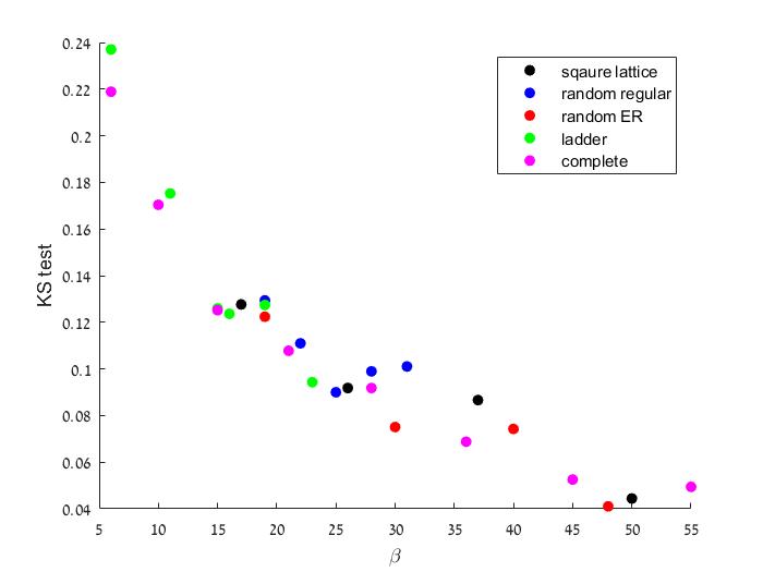
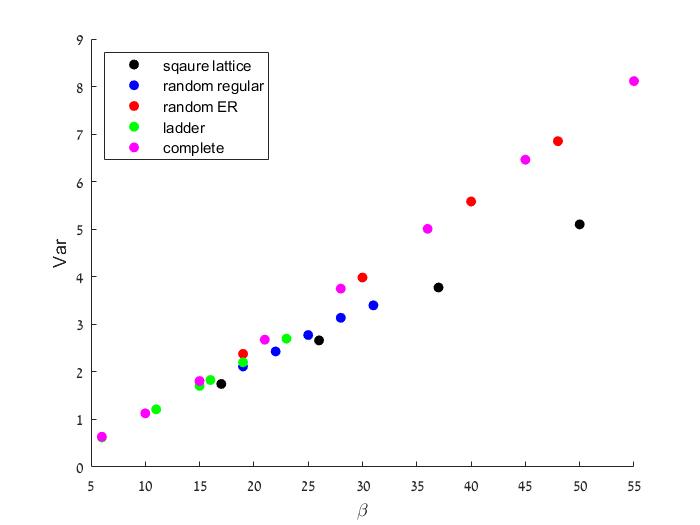
Figure 9.1. The results of several numerical experiments of growing families of graphs. For each graph we choose edge lengths at random and compute its nodal count statistics using $10^{6}$ eigenfunctions. The families of graphs we examine are complete graphs, ladder graphs, square lattices of the form $\mathbb{Z}^{2}/n\mathbb{Z}^{2}$, random Erdos-Reny graphs and random regular graphs. In the upper picture, the convergence to Gaussian is presented by means of the values of Kolmogorov–Smirnov tests versus $\beta$. In the lower picture, the variance growth in $\beta$ is presented.

Definition 9.2.

We say that a graph $\Gamma$ is a finite (3,1)-regular tree if it is a (finite) tree with $\mathrm{deg}(v)=3$ for every $v\in\mathcal{V}_{in}$. We say that a graph $\Gamma$ is a tree of cycles if it has an edge separation decomposition $\left[\Gamma_{1},\Gamma_{2}...\Gamma_{m}\right]$ where every $\Gamma_{j}$ has first Betti number $\beta_{j}=1$. See Figure 9.2 for example.

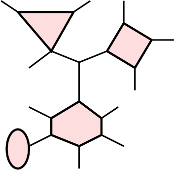
Figure 9.2. On the left, a (3,1)-regular tree. On the right, a tree of cycles, with cycles filled for emphasis.  

The following theorem combines Theorem 2.3 of [8] and Theorem 3.7 [6].

Theorem 9.3.

Let $\Gamma_{\vec{l}}$ be a standard graph and assume that $\vec{l}$ is rationally independent. Then,

1. If $\Gamma_{\vec{l}}$ is a tree of cycles, then the nodal surplus distribution is binomial,

   $$\sigma\sim Bin\left(\beta,\frac{1}{2}\right).$$

   That is:

   (9.1) $$\forall j\in\left\{0,1,...,\beta\right\}\,\,P\left(\sigma-j\right)={\beta\choose j}2^{-\beta}.$$

2. If $\Gamma_{\vec{l}}$ is a (3,1)-regular finite tree, then the Neumann surplus distribution is given by $\omega+\left|\mathcal{V}_{in}\right|+1\sim Bin\left(\left|\mathcal{V}_{in}\right|,\frac{1}{2}\right)$. That is:

   $$\forall j\in\left\{-\left|\mathcal{V}_{in}\right|-1,...,-1\right\}\,\,\,\mathrm{P}(\omega=j)=\binom{\left|\mathcal{V}_{in}\right|}{j+\left|\mathcal{V}_{in}\right|+1}2^{-\left|\mathcal{V}_{in}\right|}.$$

It is now straightforward, using central limit theorem, that the nodal surplus distributions of trees of cycles converge to a Gaussian limit. We also know that their variance in such case is $\frac{\beta}{4}$.

Corollary 9.4.

Conjecture 9.1 holds in the case where the graphs are trees of cycles.

As we said, the proof of Theorem 9.3 relies on breaking of $\sigma$ into sum of local indices and the breaking of $\omega$ into a sum of spectral positions of Neumann domains. The common feature of both is that in the cases above each of these local random variables gets only two values. A random variable $X$ that takes only two values, 0 and 1, is called a Bernoulli random variable. We will now define cut-flips on tree graphs and provide a lemma regarding the action of cut-flips on Bernoulli random variables.

Definition 9.5.

Let $\Gamma$ be a tree graph, consider a subset of vertices $\mathcal{V}_{0}\subseteq\mathcal{V}$, and the binary set $\left\{0,1\right\}^{\mathcal{V}_{0}}$. Let $u\in\mathcal{V}$ (may or may not be in $\mathcal{V}_{0}$) with edge $e\in\mathcal{E}_{v}$ and decomposition $\Gamma\setminus e=\Gamma_{1}\sqcup\Gamma_{2}$ such that $u\in\Gamma_{1}$.
We define the cut-flip $g_{u,e}:\left\{0,1\right\}^{\mathcal{V}_{0}}\rightarrow\left\{0,1\right\}^{\mathcal{V}_{0}}$, as seen in Figure 9.3, such that

$$\forall s\in\left\{0,1\right\}^{\mathcal{V}_{0}},\,\,\forall v\in\mathcal{V}_{0}\,\,\,\,\,\,\left(g_{u,e}.s\right)_{v}=\begin{cases}s_{v}&v\in\Gamma_{1}\\ 1-s_{v}&v\in\Gamma_{2}\end{cases}.$$

Namely, $g_{u,e}$ fixes the values of $s$ on $\mathcal{V}_{0}\cap\Gamma_{1}$ and “flips” the values on $\mathcal{V}_{0}\cap\Gamma_{2}$.

Lemma 9.6.

Let $\Gamma$ be a tree graph and consider a subset of vertices $\mathcal{V}_{0}\subseteq\mathcal{V}$ with Bernoulli random variables $\left\{X_{v}\right\}_{v\in\mathcal{V}_{0}}$ assigned to $\mathcal{V}_{0}$. That is, each $X_{v}$ takes the values 0 and 1, and their joint random vector $\vec{X}$ takes its values in $\left\{0,1\right\}^{\mathcal{V}_{0}}$. We do not assume that the $X_{v}$’s are identical nor that they are independent.

If the joint probability distribution is invariant under all cut-flips, namely

(9.2) $$\forall s\in\left\{0,1\right\}^{\mathcal{V}_{0}},\,\forall u\in\mathcal{V},\,\forall e\in\mathcal{E}_{u}\,\,\,\,\,\,P\left(\vec{X}=s\right) =P\left(\vec{X}=g_{u,e}.s\right),$$

then $\left|\vec{X}\right|:=\sum_{v\in\mathcal{V}_{0}}X_{v}$, has binomial distribution $X\sim Bin\left(\left|\mathcal{V}_{0}\right|,\frac{1}{2}\right)$.

Proof.

Let $e$ be an edge connecting the vertices $u_{1}$ and $u_{2}$. Observe that applying both cut flips of that edge, $TF:=g_{u_{1},e}\circ g_{u_{1},e}$ gives a total flip:

$$\forall s\in\left\{0,1\right\}^{\mathcal{V}_{0}},\,\,\forall v\in\mathcal{V}_{0}\,\,\,\left(TF.s\right)_{v}=\left(g_{u_{1},e}.\left(g_{u_{2},e}.s\right)\right)=1-s_{v}.$$

As demonstrated in Figure 9.3, given some $u\in\mathcal{V}_{0}$, applying a total flip and then each $g_{u,e}$ for all $e\in\mathcal{E}_{v}$, will result in a single flip, $F_{u}$, flipping only $u$:

$$\forall s\in\left\{0,1\right\}^{\mathcal{V}_{0}},\,\,\forall v\in\mathcal{V}_{0}\,\,\,\left(F_{u}.s\right)_{v}=\begin{cases}1-s_{v}&v=u\\ s_{v}&v\neq u\end{cases}.$$

Therefore, the group generated by all cut-flips $\left\langle\left\{g_{u,e}\right\}_{u\in\mathcal{V},\,e\in\mathcal{E}_{u}}\right\rangle$ contains every single flip and therefore acts transitively on $\left\{0,1\right\}^{\mathcal{V}_{0}}$. To see that, consider any two distinct elements $s,s^{\prime}\in\left\{0,1\right\}^{\mathcal{V}_{0}}$ and let $\left\{v_{j}\right\}_{j=1}^{n}$ be the vertices in $\mathcal{V}_{0}$ on which $s_{v_{j}}\neq s^{\prime}_{v_{j}}$. Let $g$ be the decomposition of all single flips $F_{v_{j}}$, then clearly $g\in\left\langle\left\{g_{u,e}\right\}_{u\in\mathcal{V},\,e\in\mathcal{E}_{u}}\right\rangle$ and $g.s=s^{\prime}$. Therefore, $\left\langle\left\{g_{u,e}\right\}_{u\in\mathcal{V},\,e\in\mathcal{E}_{u}}\right\rangle$ acts transitively on $\left\{0,1\right\}^{\mathcal{V}_{0}}$, and since $\vec{X}$ takes values in $\left\{0,1\right\}^{\mathcal{V}_{0}}$ with probability which is invariant under the action of $\left\langle\left\{g_{u,e}\right\}_{u\in\mathcal{V},\,e\in\mathcal{E}_{u}}\right\rangle$ then $\vec{X}$ must be uniform. To see that, consider $s,s^{\prime}\in\left\{0,1\right\}^{\mathcal{V}_{0}}$ and $g\in\left\langle\left\{g_{u,e}\right\}_{u\in\mathcal{V},\,e\in\mathcal{E}_{u}}\right\rangle$ as before, such that $g.s=s^{\prime}$. Since the probability is invariant under $g$, then

$$P\left(\vec{X}=s\right)=P\left(\vec{X}=g.s\right)=P\left(\vec{X}=s^{\prime}\right),$$

and since this is true for any $s$ and $s^{\prime}$, then

$$\forall s\in\left\{0,1\right\}^{\mathcal{V}_{0}}\,\,\,P\left(\vec{X}=s\right)=\frac{1}{\left|\left\{0,1\right\}^{\mathcal{V}_{0}}\right|}=2^{-\left|\mathcal{V}_{0}\right|}.$$

As the probability of the sum, $P\left(\left|\vec{X}\right|=j\right)$, is given by summing the probabilities of all elements $s\in\left\{0,1\right\}^{\mathcal{V}_{0}}$ for which $\sum_{v\in\mathcal{V}_{0}}s_{v}=j$, then clearly,

$$P\left(\left|\vec{X}\right|=j\right)={\left|\mathcal{V}_{0}\right|\choose j}2^{-\left|\mathcal{V}_{0}\right|}.$$

∎

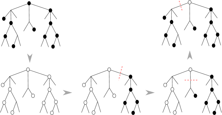
Figure 9.3. A tree with a subset of vertices of two colors, white or black. Starting with a configuration of all blacks, the first step is a total flip. The second, third and forth steps are cut flips, according to the dashed lines, that keep the root vertex unchanged. The result is a flip only of the root vertex.

We will now show that $\mathcal{R}_{v,e}:\Sigma_{\mathcal{G}}\rightarrow\Sigma_{\mathcal{G}}$, that was defined in Definition 4.40 by

$$\mathcal{R}_{v,e}\left(\vec{\kappa}_{1},\kappa_{e},\vec{\kappa}_{2}\right):=\left\{\left(\vec{\kappa}_{1},\kappa_{e}+\Theta_{2}\left(\vec{\kappa}_{2}\right),\mathcal{I}\left(\vec{\kappa}_{2}\right)\right)\right\},$$

is acting similarly to a cut-flip on the level sets of the local random variables $\boldsymbol{N}_{u}$ and $\boldsymbol{\iota}_{j}$ (see Definitions 7.4 and 8.15).

Lemma 9.7.

Let $\Gamma$ be a graph, let $e$ be a bridge with a bridge decomposition
$\Gamma\setminus e=\Gamma_{1}\sqcup\Gamma_{2}$ and let $v$ be the vertex connecting $e$ to $\Gamma_{1}$.Then,

1. For any interior vertex $u\in\mathcal{V}_{in}$,

   $$\boldsymbol{N}_{u}\circ\mathcal{R}_{v,e}=\begin{cases}\boldsymbol{N}_{u}&u\in\mathcal{V}_{1}\\ \mathrm{deg}(u)-\boldsymbol{N}_{u}&u\notin\mathcal{V}_{1}.\end{cases}$$

2. If $\Gamma$ has further edge separation $\left[\Gamma_{1,1},\Gamma_{1,2},...\Gamma_{1,m_{1}},\Gamma_{2,1},\Gamma_{2,2}...\Gamma_{2,m_{2}}\right]$, such that $\Gamma_{1,j}\subset\Gamma_{1}$ and $\Gamma_{2,i}\subset\Gamma_{2}$. Then the corresponding local magnetic indices $\boldsymbol{\iota}_{1,j}$ and $\boldsymbol{\iota}_{2,i}$ satisfy

   $$\boldsymbol{\iota}_{1,j}\circ\mathcal{R}_{v,e} =\boldsymbol{\iota}_{1,j}$$

   $$\boldsymbol{\iota}_{2,i}\circ\mathcal{R}_{v,e} =\beta_{2,i}-\boldsymbol{\iota}_{2,i}.$$

   Where $\beta_{2,i}$ is the first Betti number of $\Gamma_{2,i}$.

Proof.

In order to prove (1), let $\vec{\kappa}\in\Sigma_{\mathcal{G}}$ and notice that according to Lemma 4.42, for any $e^{\prime}\in\mathcal{E}_{u}$,

$$f_{\mathcal{R}_{v,e}\left(\vec{\kappa}\right)}\left(u\right)\partial_{e^{\prime}}f_{\mathcal{R}_{v,e}\left(\vec{\kappa}\right)}\left(u\right)=\begin{cases}f_{\vec{\kappa}}\left(u\right)\partial_{e^{\prime}}f_{\vec{\kappa}}\left(u\right)&u\in\mathcal{V}_{1}\\ -f_{\vec{\kappa}}\left(u\right)\partial_{e^{\prime}}f_{\vec{\kappa}}\left(u\right)&u\notin\mathcal{V}_{1}.\end{cases}$$

Therefore,

$$\boldsymbol{N}_{u}\left(\mathcal{R}_{v,e}\left(\vec{\kappa}\right)\right) =\frac{\mathrm{deg}(u)}{2}-\frac{1}{2}\sum_{e^{\prime}\in\mathcal{E}_{u}}\mathrm{sign}\left(f_{\mathcal{R}_{v,e}\left(\vec{\kappa}\right)}\left(u\right)\partial_{e^{\prime}}f_{\mathcal{R}_{v,e}\left(\vec{\kappa}\right)}\left(u\right)\right)$$

$$= \begin{cases}\frac{\mathrm{deg}(u)}{2}-\frac{1}{2}\sum_{e^{\prime}\in\mathcal{E}_{u}}\mathrm{sign}\left(f_{\vec{\kappa}}\left(u\right)\partial_{e^{\prime}}f_{\vec{\kappa}}\left(u\right)\right)&u\in\mathcal{V}_{1}\\ \frac{\mathrm{deg}(u)}{2}+\frac{1}{2}\sum_{e^{\prime}\in\mathcal{E}_{u}}\mathrm{sign}\left(f_{\vec{\kappa}}\left(u\right)\partial_{e^{\prime}}f_{\vec{\kappa}}\left(u\right)\right)&u\notin\mathcal{V}_{1}.\end{cases}$$

$$= \begin{cases}\boldsymbol{N}_{u}\left(\vec{\kappa}\right)&u\in\mathcal{V}_{1}\\ \mathrm{deg}(u)-\boldsymbol{N}_{u}\left(\vec{\kappa}\right)&u\notin\mathcal{V}_{1}.\end{cases}.$$

In order to prove (2), let $\vec{\kappa}=\left(\vec{\kappa}_{1},\kappa_{e},\vec{\kappa}_{2}\right)\in\Sigma_{\mathcal{G}}$ and consider the block decomposition of $\frac{\mathrm{Hess}_{\vec{\alpha}}F}{p}$ into $\frac{\mathrm{Hess}_{\vec{\alpha}_{1}}F}{p}$ and $\frac{\mathrm{Hess}_{\vec{\alpha}_{2}}F}{p}$. In Lemma 4.15 we showed that

$$\frac{\partial F}{\partial\kappa_{e}}\left(\vec{\kappa}\right)= p\left(\vec{\kappa}\right)\left(m_{\vec{\kappa}}\right)_{e},\,\,and\,so$$

$$\frac{\partial F}{\partial\kappa_{e}}\left(\mathcal{R}_{v,e}\left(\vec{\kappa}\right)\right)= p\left(\mathcal{R}_{v,e}\left(\vec{\kappa}\right)\right)\left(m_{\mathcal{R}_{v,e}\left(\vec{\kappa}\right)}\right)_{e},$$

where both $\left(m_{\vec{\kappa}}\right)_{e}$ and $\left(m_{\mathcal{R}_{v,e}\left(\vec{\kappa}\right)}\right)_{e}$ are strictly positive (since $\vec{\kappa}\in\Sigma_{\mathcal{G}}$). Denote the positive scalar $c:=\frac{\left(m_{\mathcal{R}_{v,e}\left(\vec{\kappa}\right)}\right)_{e}}{\left(m_{\vec{\kappa}}\right)_{e}}$. As $\mathcal{R}_{v,e}\left(\vec{\kappa}\right)=\left(\vec{\kappa}_{1},\tilde{\kappa_{e}},\mathcal{I}\left(\vec{\kappa}_{2}\right)\right)$ for some $\tilde{\kappa_{e}}$, then $\vec{\kappa}$ and $\mathcal{R}_{v,e}\left(\vec{\kappa}\right)$ agree on their $\vec{\kappa}_{1}$ coordinates. It then follows from Proposition 8.17 that,

$$\frac{\mathrm{Hess}_{\vec{\alpha}_{1}}F}{\frac{\partial F}{\partial\kappa_{e}}}\left(\mathcal{R}_{v,e}\left(\vec{\kappa}\right)\right)=\frac{\mathrm{Hess}_{\vec{\alpha}_{1}}F}{\frac{\partial F}{\partial\kappa_{e}}}\left(\vec{\kappa}\right),$$

which means that

$$\frac{\mathrm{Hess}_{\vec{\alpha}_{1}}F}{p}\left(\mathcal{R}_{v,e}\left(\vec{\kappa}\right)\right)=c\frac{\mathrm{Hess}_{\vec{\alpha}_{1}}F}{p}\left(\vec{\kappa}\right).$$

Therefore, the Morse indices of their sub-block agree:

$$\boldsymbol{\iota}_{1,j}\left(\mathcal{R}_{v,e}\left(\vec{\kappa}\right)\right)=\mathcal{M}\left(-\frac{\mathrm{Hess}_{\vec{\alpha}_{1,j}}F}{p}\left(\mathcal{R}_{v,e}\left(\vec{\kappa}\right)\right)\right)=\mathcal{M}\left(-c\frac{\mathrm{Hess}_{\vec{\alpha}_{1,j}}F}{p}\left(\vec{\kappa}\right)\right)=\boldsymbol{\iota}_{1,j}\left(\vec{\kappa}\right),$$

In the same way, $\mathcal{I}\left(\vec{\kappa}\right)$ and $\mathcal{R}_{v,e}\left(\vec{\kappa}\right)$ agree on their $\vec{\kappa}_{2}$ coordinates, so

$$\frac{\mathrm{Hess}_{\vec{\alpha}_{2}}F}{\frac{\partial F}{\partial\kappa_{e}}}\left(\mathcal{R}_{v,e}\left(\vec{\kappa}\right)\right)=\frac{\mathrm{Hess}_{\vec{\alpha}_{2}}F}{\frac{\partial F}{\partial\kappa_{e}}}\left(\mathcal{I}\vec{\kappa}\right)=-\frac{\mathrm{Hess}_{\vec{\alpha}_{2}}F}{\frac{\partial F}{\partial\kappa_{e}}}\left(\vec{\kappa}\right),$$

using Proposition 8.17 once more, for the inversion. Therefore,

$$\boldsymbol{\iota}_{2,i}\left(\mathcal{R}_{v,e}\left(\vec{\kappa}\right)\right)=\mathcal{M}\left(-\frac{\mathrm{Hess}_{\vec{\alpha}_{2,i}}F}{p}\left(\mathcal{R}_{v,e}\left(\vec{\kappa}\right)\right)\right)=\mathcal{M}\left(c\frac{\mathrm{Hess}_{\vec{\alpha}_{2,i}}F}{p}\left(\vec{\kappa}\right)\right)=\beta_{2,i}-\boldsymbol{\iota}_{2,i}\left(\vec{\kappa}\right).$$

∎

Using both Lemmas 9.6 and 9.7, we can prove Theorem 9.3. Let us first consider the Neumann case.

9.1. Proof of Theorem 9.3 (2).

Let $\Gamma_{\vec{l}}$ be a (3,1)-regular finite tree with rationally independent $\vec{l}$. Consider the subset of interior vertices $\mathcal{V}_{0}=\mathcal{V}_{in}$ and define $X_{v}:=\boldsymbol{N}_{v}-1$ for any $v\in\mathcal{V}_{in}$ such that $\left\{X_{v}\right\}_{v\in\mathcal{V}_{in}}$ are random variables on $\Sigma_{\mathcal{G}}$ with Borel $\sigma$-algebra and BG measure $\frac{1}{\mu_{\vec{l}}\left(\Sigma_{\mathcal{G}}\right)}\mu_{\vec{l}}$. According to Proposition 7.6 and since every $v\in\mathcal{V}_{in}$ is of $\mathrm{deg}(v)=3$, then $\boldsymbol{N}_{v}$ takes the values $1$ and $2$ and therefore $X_{v}$ takes the values 0 and 1, and is therefore Bernoulli random variable. Consider $v\in\mathcal{V},\,e\in\mathcal{E}_{v}$ and the partition $\Gamma\setminus\left\{e\right\}=\Gamma_{1}\sqcup\Gamma_{2}$ such that $v\in\Gamma_{1}$, with corresponding cut-flip $g_{v,e}$ (as defined in Lemma 9.6). Consider the level sets

$$\forall s\in\left\{0,1\right\}^{\mathcal{V}_{0}}\,\,\,\vec{X}^{-1}\left(s\right):=\left\{\vec{\kappa}\in\Sigma_{\mathcal{G}}\,\,:\,\,\forall v\in\mathcal{V}_{0}\,\,\,X_{v}\left(\vec{\kappa}\right)=s_{v}\right\}.$$

According to Lemma 9.7,

$$X_{u}\left(\mathcal{R}_{v,e}\left(\vec{\kappa}\right)\right) =\begin{cases}X_{u}\left(\vec{\kappa}\right)&u\in\Gamma_{1}\\ 1-X_{u}\left(\vec{\kappa}\right)&u\in\Gamma_{2}\end{cases},$$

and a simple observation leads to

$$\forall s\in\left\{0,1\right\}^{\mathcal{V}_{0}}\,\,\,\,\mathcal{R}_{v,e}\left(\vec{X}^{-1}\left(s\right)\right)=\vec{X}^{-1}\left(g_{v,e}.s\right).$$

By Lemma 4.42, $\mathcal{R}_{v,e}$ is $\mu_{\vec{l}}$ preserving and therefore

$$\forall s\in\left\{0,1\right\}^{\mathcal{V}_{0}}\,\,\,\,P\left(\vec{X}=s\right)= \frac{\mu_{\vec{l}}\left(\vec{X}^{-1}\left(s\right)\right)}{\mu_{\vec{l}}\left(\Sigma_{\mathcal{G}}\right)}$$

$$= \frac{\mu_{\vec{l}}\left(\mathcal{R}_{v,e}\left(\vec{X}^{-1}\left(s\right)\right)\right)}{\mu_{\vec{l}}\left(\Sigma_{\mathcal{G}}\right)}$$

$$= \frac{\mu_{\vec{l}}\left(\vec{X}^{-1}\left(g_{v,e}.s\right)\right)}{\mu_{\vec{l}}\left(\Sigma_{\mathcal{G}}\right)}$$

$$= P\left(\vec{X}=g_{v,e}.s\right).$$

Therefore, by Lemma 9.6, $\left|\vec{X}\right|:=\sum_{v\in\mathcal{V}_{in}}X_{u}$ is binomial $\left|\vec{X}\right|\sim Bin\left(\left|\mathcal{V}_{in}\right|,\frac{1}{2}\right)$. According to Proposition 7.12 and Lemma 7.5, for every $n\in\mathcal{G}$ such that $n>2\frac{L}{L_{min}}$,

(9.3) $$\sum_{u\in\mathcal{V}_{in}}\boldsymbol{N}_{u}\left(\left\{k_{n}\vec{l}\right\}\right)=\phi\left(f_{n}\right)-\mu\left(f_{n}\right)+E-\left|\partial\Gamma\right|.$$

Since $\Gamma$ is a tree, then $\phi\left(f_{n}\right)=n$, and therefore $\phi\left(f_{n}\right)-\mu\left(f_{n}\right)=-\omega\left(f_{n}\right)$ which is equal to $\boldsymbol{\omega}\left(\left\{k_{n}\vec{l}\right\}\right)$ (by Lemma 6.13). As all $\boldsymbol{N}_{u}$’s and $\boldsymbol{\omega}$ are constant on connected components, and $\left\{k_{n}\vec{l}\right\}$ is dense in $\Sigma$ (Theorem 4.32), then the following relation holds on $\Sigma_{\mathcal{G}}$:

$$\boldsymbol{\omega}=-\sum_{u\in\mathcal{V}_{in}}\boldsymbol{N}_{u}+E-\left|\partial\Gamma\right|.$$

In particular, since $\Gamma$ is a tree so $E-V=-1$, we get

$$\boldsymbol{\omega}=-\sum_{u\in\mathcal{V}_{in}}X_{u}+E-V=-\left|\vec{X}\right|-1.$$

We may now deduce that $-\boldsymbol{\omega}-1\sim Bin\left(\left|\mathcal{V}_{in}\right|,\frac{1}{2}\right)$ and therefore so does $\left|\mathcal{V}_{in}\right|-\left(-\boldsymbol{\omega}-1\right)=\boldsymbol{\omega}+\left|\mathcal{V}_{in}\right|+1$. This proves that

$$\forall j\in\left\{-\left|\mathcal{V}_{in}\right|-1,...,-1\right\}\ \ \ \,\,\,\frac{\mu_{\vec{l}}\left(\boldsymbol{\omega}^{-1}\left(j\right)\right)}{\mu_{\vec{l}}\left(\Sigma_{\mathcal{G}}\right)}=\binom{\left|\mathcal{V}_{in}\right|}{j+\left|\mathcal{V}_{in}\right|+1}2^{-\left|\mathcal{V}_{in}\right|}.$$

This is the needed result as the Neumann surplus probability is given by

$$P\left(\omega=j\right)=\frac{\mu_{\vec{l}}\left(\boldsymbol{\omega}^{-1}\left(j\right)\right)}{\mu_{\vec{l}}\left(\Sigma_{\mathcal{G}}\right)}.$$

9.2. Proof of Theorem 9.3 (1).

Let $\Gamma_{\vec{l}}$ be a standard graph with rationally independent $\vec{l}$, and assume it is a tree of cycles. Denote the set of bridges by $\mathcal{E}_{bridges}$, and consider the edge separation $\left[\Gamma_{1},\Gamma_{2}...\Gamma_{m}\right]$. As $\Gamma_{\vec{l}}$ is a tree of cycles, then $m=\beta$ and each $\Gamma_{j}$ has first Betti number $\beta_{j}=1$. It now follows from Theorem 8.13 that every $\boldsymbol{\iota}_{j}$ satisfies

$$\frac{1}{\mu_{\vec{l}}\left(\Sigma_{\mathcal{G}}\right)}\mu_{\vec{l}}\left(\boldsymbol{\iota}_{j}^{-1}\left(0\right)\right)=\frac{1}{\mu_{\vec{l}}\left(\Sigma_{\mathcal{G}}\right)}\mu_{\vec{l}}\left(\boldsymbol{\iota}_{j}^{-1}\left(1\right)\right)=\frac{1}{2}.$$

Consider $\left\{\boldsymbol{\iota}_{j}\right\}_{j=1}^{\beta}$ as random variables over $\Sigma_{\mathcal{G}}$ with Borel $\sigma$-algebra and probability measure $\frac{1}{\mu_{\vec{l}}\left(\Sigma_{\mathcal{G}}\right)}\mu_{\vec{l}}$. Let $\tilde{\Gamma}$ be an auxiliary graph whose edges are $\mathcal{E}_{edges}$ and whose vertices are the connected components of $\Gamma\setminus\mathcal{E}_{edges}$ and let $\mathcal{V}_{0}=\left\{v_{j}\right\}_{j=1}^{\beta}$ be the vertices corresponding to the non-trivial connected components $\left\{\Gamma_{j}\right\}_{j=1}^{\beta}$, as demonstrated in Figure 9.4. Clearly by the construction, $\tilde{\Gamma}$ is a tree. Let $\left\{\boldsymbol{\iota}_{j}\right\}_{v_{j}\in\mathcal{V}_{0}}$ be the random variables associated to the vertices in $\mathcal{V}_{0}$ as in Lemma 9.6, with probability $P\left(\boldsymbol{\iota}_{j}=i\right)=\frac{1}{\mu_{\vec{l}}\left(\Sigma_{\mathcal{G}}\right)}\mu_{\vec{l}}\left(\boldsymbol{\iota}_{j}^{-1}\left(i\right)\right)$. Let $\vec{\boldsymbol{\iota}}$ be their joint vector, taking values in $\left\{0,1\right\}^{\beta}$, with probability given by

$$\forall s\in\left\{0,1\right\}^{\beta}\,\,P\left(\vec{\boldsymbol{\iota}}=s\right)=\frac{1}{\mu_{\vec{l}}\left(\Sigma_{\mathcal{G}}\right)}\mu_{\vec{l}}\left(\cap_{v_{j}\in\mathcal{V}_{0}}\boldsymbol{\iota}_{j}^{-1}\left(s_{v_{j}}\right)\right).$$

Let $e\in\mathcal{E}_{bridges}$ and let $v\in\mathcal{V}$ be a vertex of $\Gamma$ connected to $e$ with $\tilde{v}\in\tilde{\mathcal{V}}$ being the corresponding vertex of $\tilde{\Gamma}$ (the connected component that contain $v$). Consider the bridge decomposition $\tilde{\Gamma}\setminus\left\{e\right\}=\tilde{\Gamma}_{1}\sqcup\tilde{\Gamma}_{2}$ such that $\tilde{v}\in\tilde{\Gamma}_{1}$, and let $g_{\tilde{v},e}$ be the corresponding cut-flip (on $\tilde{\Gamma}$). It follows from Lemma 9.7, that every $\boldsymbol{\iota}_{j}$ satisfies:

$$\boldsymbol{\iota}_{j}\left(\mathcal{R}_{v,e}\left(\vec{\kappa}\right)\right)= \begin{cases}\boldsymbol{\iota}_{j}\left(\vec{\kappa}\right)&v_{j}\in\tilde{\Gamma}_{1}\\ 1-\boldsymbol{\iota}_{j}\left(\vec{\kappa}\right)&v_{j}\in\tilde{\Gamma}_{2}\end{cases},$$

and exactly as in the proof of Theorem 9.3 (2), it follows that

$$\forall s\in\left\{0,1\right\}^{\beta}\,\,\,\,\mathcal{R}_{v,e}\left(\vec{\boldsymbol{\iota}}^{-1}\left(s\right)\right)=\vec{\boldsymbol{\iota}}^{-1}\left(g_{\tilde{v},e}.s\right),$$

which leads to

$$\forall s\in\left\{0,1\right\}^{\beta}\,\,\,\,P\left(\vec{\boldsymbol{\iota}}=s\right)=P\left(\vec{\boldsymbol{\iota}}=g_{\tilde{v},e}.s\right).$$

And then Lemma 9.6 can be applied to show that the sum $\left|\vec{\boldsymbol{\iota}}\right|=\sum_{j=1}^{\beta}\boldsymbol{\iota}_{j}$ has binomial distribution $\left|\vec{\boldsymbol{\iota}}\right|\sim Bin\left(\beta,\frac{1}{2}\right)$. By Corollary 8.18, $\boldsymbol{\sigma}=\sum_{j=1}^{\beta}\boldsymbol{\iota}_{j}=\left|\vec{\boldsymbol{\iota}}\right|$ which means that $\boldsymbol{\sigma}\sim Bin\left(\beta,\frac{1}{2}\right)$. So,

$$\forall j\in\left\{0,1,...\beta\right\}\,\,\frac{1}{\mu_{\vec{l}}\left(\Sigma_{\mathcal{G}}\right)}\mu_{\vec{l}}\left(\boldsymbol{\sigma}^{-1}\left(j\right)\right)={\beta\choose j}2^{-\beta},$$

as needed since $P\left(\sigma=j\right)=\frac{1}{\mu_{\vec{l}}\left(\Sigma_{\mathcal{G}}\right)}\mu_{\vec{l}}\left(\boldsymbol{\sigma}^{-1}\left(j\right)\right)$.

Figure 9.4. On the left, $\Gamma$ a tree of cycles, with cycles filled for emphasis. On the right, $\tilde{\Gamma}$ the constructed tree, with the corresponding $\mathcal{V}_{0}$ chosen vertices marked by circles.

10. Summary

This thesis deals with generic eigenfunctions of standard graphs and the statistics of their nodal and Neumann counts. The nodal count $\phi(n)$ is the number of points where the nth eigenfunction vanishes. The Neumann count $\mu(n)$ is the number of local extrema of the nth eigenfunction. Both nodal and Neumann counts cannot be defined on every eigenfunction and we restrict the discussion to generic eigenfunctions on which the two counts are well defined. We call an eigenfunction generic if it corresponds to a simple eigenvalue, does not vanish on vertices, and its outgoing derivatives at every interior vertex do not vanish as well.

The first main result of this thesis, Theorem 5.5, is a generalization of the genericity results in [36, 67], in which we justify the generality of our discussion. We prove, using two different notions of genericity, that generically every eigenfunction which is not supported on a loop (if such exist) is generic and therefore has well defined nodal and Neumann counts. Given a standard quantum graph $\Gamma_{\vec{l}{}}$, we denote the index set of $n$’s for which the nth eigenfunction is generic by $\mathcal{G}$, and we denote its intersection with $\{1,2,...N\}$ by $\mathcal{G}(N)$. As was shown in [27, 73], the nodal surplus $\sigma(n):=\phi(n)-n$ is uniformly bounded between $0$ and $\beta$, the first Betti number of the graph. Therefore, the statistics of the nodal count is encapsulated in the nodal surplus distribution. The nodal surplus distribution is well defined if the following limits exist for any $j\in\{0,1,...\beta\}$:

(10.1) $$P\left(\sigma=j\right) :=\lim_{N\rightarrow\infty}\frac{\left|\left\{n\in\mathcal{G}\left(N\right)\,\,:\,\,\sigma(n)=j\right\}\right|}{\left|\mathcal{G}\left(N\right)\right|}$$

Similarly, we define the Neumann surplus $\omega(n):=\mu(n)-n$ and in Theorem 3.4 we provide a uniform bound:

(10.2) $$\forall n\in\mathcal{G}\,\,\,\,\,\,\,\,1-\beta-\left|\partial\Gamma\right|\leq\omega(n)\leq 2\beta-1.$$

Hence, the Neumann count statistics is described by the Neumann surplus distribution, which is well defined if the following limits exist for any $j$ in the allowed range of $\omega$:

(10.3) $$P\left(\omega=j\right) :=\lim_{N\rightarrow\infty}\frac{\left|\left\{n\in\mathcal{G}\left(N\right)\,\,:\,\,\omega(n)=j\right\}\right|}{\left|\mathcal{G}\left(N\right)\right|}$$

The second main result of this thesis is Theorem 6.5, in which we prove that if the edge lengths of the graph are rationally independent then the above limits exist and so the nodal and Neumann surplus distributions are well defined. We do so by providing a probabilistic setting for the statistical discussion. We define a $\sigma$-algebra $\mathcal{F}_{\mathcal{G}}$ on $\mathcal{G}$ such that $d_{\mathcal{G}}$ the (restricted) natural density is a measure on $(\mathcal{G},\mathcal{F}_{\mathcal{G}})$. We then prove that the functions $\sigma,\omega:\mathcal{G}\rightarrow\mathbb{Z}$ are (finite) random variables on $(\mathcal{G},\mathcal{F}_{\mathcal{G}},d_{\mathcal{G}})$. This proves that the distributions are well defined, and moreover, it allows to consider their joint distribution. In Theorem 6.5 we also show that both $\sigma$ and $\omega$ are symmetric around $\frac{\beta}{2}$ and $\frac{\beta-\left|\partial\Gamma\right|}{2}$ simultaneously. That is,

(10.4) $$P\left((\sigma,\omega)=(j,i)\right) =P\left((\sigma,\omega)=(\beta-j,\beta-\left|\partial\Gamma\right|-i)\right).$$

As a corollary, if the edge lengths of a graph are rationally independent then both $\beta$ and $\left|\partial\Gamma\right|$ can be obtained by the averages of the nodal and Neumann surplus distributions:

$$\beta=2\mathbb{E}\left(\sigma\right) =\lim_{N\rightarrow\infty}\frac{2}{\left|\mathcal{G}(N)\right|}\sum_{n\in\mathcal{G}(N)}\sigma(n),\,\,\text{and}$$

$$\left|\partial\Gamma\right|=2\mathbb{E}\left(\sigma-\omega\right) =\lim_{N\rightarrow\infty}\frac{2}{\left|\mathcal{G}(N)\right|}\sum_{n\in\mathcal{G}(N)}(\sigma(n)-\omega(n)).$$

There are two immediate consequences of the above, regarding the "geometric information" of the graph that is stored in the nodal and Neumann counts. The first, is that although counting zero points and counting extrema seems equivalent, it is not. For example consider tree graphs, so that $\sigma\equiv 0$ and cannot distinguish between different trees, but the average Neumann surplus distinguishes between trees of different $\left|\partial\Gamma\right|$. The second consequence is that given both the average nodal surplus and the average Neumann surplus, we obtain $\beta$ and $\left|\partial\Gamma\right|$. It can be shown that there are finitely many discrete graphs with a given $\beta$ and $\left|\partial\Gamma\right|$, and so the inverse question of retrieving the underlying discrete is narrowed down to a finite set of graphs, given only the averages of the nodal and Neumann surpluses.

The third main result is Theorem 9.3 in which we explicitly calculate the nodal and Neumann surplus distributions for two specific families of graphs. If a graph is a tree of cycles (see Definition LABEL:def:_tree_of_cycles) with rationally independent edge lengths, then its nodal surplus distribution is binomial,

$$\sigma\sim Bin\left(\beta,\frac{1}{2}\right).$$

If a graph is a (3,1)-regular finite tree (see Definition LABEL:def:_tree_of_cycles) with rationally independent edge lengths then its Neumann surplus distribution is a shifted binomial distribution given by

$$\omega+\left|\mathcal{V}_{in}\right|+1\sim Bin\left(\left|\mathcal{V}_{in}\right|,\frac{1}{2}\right),$$

where $\left|\mathcal{V}_{in}\right|=V-\left|\partial\Gamma\right|$ is the number of interior vertices.
The binomial distribution converge to Gaussian by the Central Limit Theorem. Therefore, the conjectured universal behavior of the nodal surplus statistics, as reformulated in Conjecture 9.1, holds for trees of cycles.

Appendix A Decomposition for a bridge

In this subsection we provide the technical details of the bridge decomposition. As already discussed, more general results can be found in Section 4 of [8]. We will follow the method of Section 4 of [8], which relies on the scattering results obtained in [15].

Let $e$ be a bridge of $\Gamma$ and consider the bridge decomposition $\Gamma\setminus\left\{e\right\}=\Gamma_{1}\sqcup\Gamma_{2}$. Denote the edges of $\Gamma_{1},\Gamma_{2}$ by $\mathcal{E}_{1},\mathcal{E}_{2}$ correspondingly. Consider the direction of $e$ from $\Gamma_{1}$ to $\Gamma_{2}$ and the basis of directed edges in the following order: directed edges of $\Gamma_{1}$, $e$, $\hat{e}$, directed edges of $\Gamma_{2}$. With this order and edge grouping the real orthogonal scattering matrix $S$ has the following block structure:

$$S=\begin{pmatrix}S_{1}&0&t_{1}&0\\ t^{\prime}_{1}&0&r_{1}&0\\ 0&r_{2}&0&t^{\prime}_{2}\\ 0&t_{2}&0&S_{2}\end{pmatrix}.$$

Where for $j\in\left\{1,2\right\}$, $S_{j}$ is square matrix of dimension $2\left|\mathcal{E}_{j}\right|$, $t_{j}$ and $t_{j}^{\prime}$ are column and row vectors of dimension $2\left|\mathcal{E}_{j}\right|$ and $r_{j}$ is a scalar. Let $\boldsymbol{z}_{1},\boldsymbol{z}_{2}$ be unitary diagonal matrices of dimensions $2\left|\mathcal{E}_{1}\right|$ and $2\left|\mathcal{E}_{2}\right|$and let $z_{e}$ be uni-modular. Consider the unitary matrix

(A.1) $$U_{\left(\boldsymbol{z}_{1},z_{e},\boldsymbol{z}_{2}\right)}:=\left(\boldsymbol{z}_{1}\oplus z_{e}\oplus z_{e}\oplus\boldsymbol{z}_{2}\right)S=\begin{pmatrix}\boldsymbol{z}_{1}S_{1}&0&\boldsymbol{z}_{1}t_{1}&0\\ z_{e}t^{\prime}_{1}&0&z_{e}r_{1}&0\\ 0&z_{e}r_{2}&0&z_{e}t^{\prime}_{2}\\ 0&\boldsymbol{z}_{2}t_{2}&0&\boldsymbol{z}_{2}S_{2}\end{pmatrix}.$$

It is apparent that $U_{\left(\boldsymbol{z}_{1},z_{e},\boldsymbol{z}_{2}\right)}$ has a special block structure, but it is not block diagonal. The following definitions are motivated by the infinite leads scattering matrix which is used in [15].

Definition A.1.

Define $D_{i}\left(\boldsymbol{z}_{i}\right):=\boldsymbol{z}_{i}S_{i}-1$ and $\mathcal{S}_{i}\left(\boldsymbol{z}_{i}\right):=r_{i}-t^{\prime}_{i}\left(D_{i}\left(\boldsymbol{z}_{i}\right)\right)^{+}\boldsymbol{z}_{i}t_{i}$ for $i\in\left\{1,2\right\}$. Where $\left(D_{i}\left(\boldsymbol{z}_{i}\right)\right)^{+}$ is the Moore-Penrose inverse and is equal to $D_{i}\left(\boldsymbol{z}_{i}\right)^{-1}$ whenever $D_{i}\left(\boldsymbol{z}_{i}\right)$ is invertible.

The definition of the Moore-Penrose inverse can be found in [53], and we will only use its following property:

Lemma A.2.

[53] Given a matrix $A$ we denote its Moore-Penrose inverse by $A^{+}$. It satisfies the property that $1-A^{+}A$ is the orthogonal projection on $\ker\left(A\right)$ and $A^{+}A$ is the orthogonal projection on $\left(\ker\left(A\right)\right)^{\perp}$.

Remark A.3.

Although it was not mentioned by name, the Moore-Penrose inverse is being used in [15].

Lemma A.4.

[8, 15] For both $i\in\left\{1,2\right\}$, $t_{i}^{\prime}\in\left(\ker\left(D_{i}\left(\boldsymbol{z}_{i}\right)\right)\right)^{\perp}$ and if $a_{1}\in\ker\left(D_{i}\left(\boldsymbol{z}_{i}\right)\right)$, then (in block structure) $\boldsymbol{a}=\begin{pmatrix}a_{1}\\ 0\\ 0\\ 0\end{pmatrix}\in\ker\left(1-U_{\left(\boldsymbol{z}_{1},z_{e},\boldsymbol{z}_{2}\right)}\right)$.

Proof.

Let $a_{1}\in\ker D_{1}\left(\boldsymbol{z}_{1}\right)$ and let $\boldsymbol{a}=\begin{pmatrix}a_{1}\\ 0\\ 0\\ 0\end{pmatrix}$. Since $D_{1}\left(\boldsymbol{z}_{1}\right)a_{1}=0$, then $\boldsymbol{z}_{1}S_{1}a_{1}=a_{1}$ and therefore, using the block structure of $U_{\left(\boldsymbol{z}_{1},z_{e},\boldsymbol{z}_{2}\right)}$,

$$U_{\left(\boldsymbol{z}_{1},z_{e},\boldsymbol{z}_{2}\right)}\boldsymbol{a}=\begin{pmatrix}\boldsymbol{z}_{1}S_{1}a_{1}\\ z_{e}t^{\prime}_{1}a_{1}\\ 0\\ 0\end{pmatrix}=\begin{pmatrix}a_{1}\\ z_{e}t^{\prime}_{1}a_{1}\\ 0\\ 0\end{pmatrix}.$$

which means that $\left\|U_{\left(\boldsymbol{z}_{1},z_{e},\boldsymbol{z}_{2}\right)}\boldsymbol{a}\right\|^{2}=\left\|a_{1}\right\|^{2}+\left\|z_{e}t^{\prime}_{1}a_{1}\right\|^{2}$. Since $U_{\left(\boldsymbol{z}_{1},z_{e},\boldsymbol{z}_{2}\right)}$ is unitary, then $\left\|U_{\left(\boldsymbol{z}_{1},z_{e},\boldsymbol{z}_{2}\right)}\boldsymbol{a}\right\|^{2}=\left\|\boldsymbol{a}\right\|^{2}=\left\|a_{1}\right\|^{2}$ and therefore $z_{e}t^{\prime}_{1}a_{1}=0$. Since $z_{e}\neq 0$ (uni-modular) then it follows that $a_{1}$, and hence $\ker D_{1}\left(\boldsymbol{z}_{1}\right)$, is orthogonal to $t_{1}^{\prime}$. In particular it follows that $U_{\left(\boldsymbol{z}_{1},z_{e},\boldsymbol{z}_{2}\right)}\boldsymbol{a}=\boldsymbol{a}$ and therefore $\boldsymbol{a}\in\ker\left(1-U_{\left(\boldsymbol{z}_{1},z_{e},\boldsymbol{z}_{2}\right)}\right)$. ∎

Lemma A.5.

[8]The determinant of $1-U_{\left(\boldsymbol{z}_{1},z_{e},\boldsymbol{z}_{2}\right)}$ can be decomposed as follows:

(A.2) $$\det\left(1-U_{\left(\boldsymbol{z}_{1},z_{e},\boldsymbol{z}_{2}\right)}\right)=\det D_{1}\left(\boldsymbol{z}_{1}\right)\cdot\det D_{2}\left(\boldsymbol{z}_{2}\right)\cdot\left(1-z_{e}^{2}\mathcal{S}\left(\boldsymbol{z}_{1}\right)\mathcal{S}\left(\boldsymbol{z}_{2}\right)\right).$$

Moreover, let

$$M:=\begin{pmatrix}D_{1}\left(\boldsymbol{z}_{1}\right)&0&\boldsymbol{z}_{1}t_{1}&0\\ 0&-1&z_{e}\mathcal{S}_{1}\left(\boldsymbol{z}_{1}\right)&0\\ 0&z_{e}\mathcal{S}_{2}\left(\boldsymbol{z}_{2}\right)&-1&0\\ 0&\boldsymbol{z}_{2}t_{2}&0&D_{2}\left(\boldsymbol{z}_{2}\right)\end{pmatrix},$$

then

(A.3) $$\ker\left(1-U_{\left(\boldsymbol{z}_{1},z_{e},\boldsymbol{z}_{2}\right)}\right)=\ker M.$$

Proof.

Let $L_{1}=\begin{pmatrix}1&0&0&0\\ -z_{e}t^{\prime}_{1}D_{1}\left(\boldsymbol{z}_{1}\right)^{+}&1&0&0\\ 0&0&1&0\\ 0&0&0&1\end{pmatrix}$ and let $L_{2}=\begin{pmatrix}1&0&0&0\\ 0&1&0&0\\ 0&0&1&-z_{e}t^{\prime}_{2}D_{2}\left(\boldsymbol{z}_{2}\right)^{+}\\ 0&0&0&1\end{pmatrix}$ so that $L_{1}L_{2}\left(U_{\left(\boldsymbol{z}_{1},z_{e},\boldsymbol{z}_{2}\right)}-1\right)$ is equal to

$$\begin{pmatrix}D_{1}\left(\boldsymbol{z}_{1}\right)&0&\boldsymbol{z}_{1}t_{1}&0\\ z_{e}t^{\prime}_{1}\left(1-D_{1}\left(\boldsymbol{z}_{1}\right)^{+}D_{1}\left(\boldsymbol{z}_{1}\right)\right)&-1&z_{e}\mathcal{S}_{1}\left(\boldsymbol{z}_{1}\right)&0\\ 0&z_{e}\mathcal{S}_{2}\left(\boldsymbol{z}_{2}\right)&-1&z_{e}t^{\prime}_{2}\left(1-D_{2}\left(\boldsymbol{z}_{2}\right)^{+}D_{2}\left(\boldsymbol{z}_{2}\right)\right)\\ 0&\boldsymbol{z}_{2}t_{2}&0&D_{2}\left(\boldsymbol{z}_{2}\right)\end{pmatrix}.$$

According to Lemma A.4, $z_{e}t^{\prime}_{i}\in\left(\ker D_{i}\left(\boldsymbol{z}_{i}\right)\right)^{\perp}$ and by Lemma A.2, $\left(1-D_{i}\left(\boldsymbol{z}_{i}\right)^{+}D_{i}\left(\boldsymbol{z}_{i}\right)\right)$ is the orthogonal projection on $\ker D_{i}\left(\boldsymbol{z}_{i}\right)$. Therefore $z_{e}t^{\prime}_{i}\left(1-D_{i}\left(\boldsymbol{z}_{i}\right)^{+}D_{i}\left(\boldsymbol{z}_{i}\right)\right)=0$ for both $i\in\left\{1,2\right\}$, and so $L_{1}L_{2}\left(U_{\left(\boldsymbol{z}_{1},z_{e},\boldsymbol{z}_{2}\right)}-1\right)=M$. Notice that both $L_{1}$ and $L_{2}$ are invertible with $\det\left(L_{1}\right)=\det\left(L_{2}\right)=1$ so left multiplication by $L_{1}L_{2}$ does not change the (right) kernel:

$$\ker\left(1-U_{\left(\boldsymbol{z}_{1},z_{e},\boldsymbol{z}_{2}\right)}\right)=\ker\left(U_{\left(\boldsymbol{z}_{1},z_{e},\boldsymbol{z}_{2}\right)}-1\right)=\ker L_{1}L_{2}\left(U_{\left(\boldsymbol{z}_{1},z_{e},\boldsymbol{z}_{2}\right)}-1\right)=\ker M,$$

and $\det M=\det\left(U_{\left(\boldsymbol{z}_{1},z_{e},\boldsymbol{z}_{2}\right)}-1\right)$. The matrix $M=L_{1}L_{2}\left(U_{\left(\boldsymbol{z}_{1},z_{e},\boldsymbol{z}_{2}\right)}-1\right)$ has triangular block structure $M=\begin{pmatrix}A&0\\ C&D\end{pmatrix}$ with blocks: $A=\begin{pmatrix}D_{1}\left(\boldsymbol{z}_{1}\right)&0&\boldsymbol{z}_{1}t_{1}\\ 0&-1&z_{e}\mathcal{S}_{1}\left(\boldsymbol{z}_{1}\right)\\ 0&z_{e}\mathcal{S}_{2}\left(\boldsymbol{z}_{2}\right)&-1\end{pmatrix}$, $B=\begin{pmatrix}0\\ 0\\ 0\end{pmatrix},\,C=\begin{pmatrix}0&\boldsymbol{z}_{2}t_{2}&0\end{pmatrix}$ and $D=D_{2}\left(\boldsymbol{z}_{2}\right)$, so $\det\left(M\right)=\det\left(A\right)\det\left(D\right).$ Namely,

$$det\left(U_{\left(\boldsymbol{z}_{1},z_{e},\boldsymbol{z}_{2}\right)}-1\right)=\det\left(D_{2}\left(\boldsymbol{z}_{2}\right)\right)\det\begin{pmatrix}D_{1}\left(\boldsymbol{z}_{1}\right)&0&\boldsymbol{z}_{1}t_{1}\\ 0&-1&z_{e}\mathcal{S}_{1}\left(\boldsymbol{z}_{1}\right)\\ 0&z_{e}\mathcal{S}_{2}\left(\boldsymbol{z}_{2}\right)&-1\end{pmatrix}.$$

Using the same argument, $A=\begin{pmatrix}D_{1}\left(\boldsymbol{z}_{1}\right)&0&\boldsymbol{z}_{1}t_{1}\\ 0&-1&z_{e}\mathcal{S}_{1}\left(\boldsymbol{z}_{1}\right)\\ 0&z_{e}\mathcal{S}_{2}\left(\boldsymbol{z}_{2}\right)&-1\end{pmatrix}$ has upper triangular blocks structure, so

$$\det\left(A\right)=\det\left(D_{1}\left(\boldsymbol{z}_{1}\right)\right)\det\begin{pmatrix}-1&z_{e}\mathcal{S}_{1}\left(\boldsymbol{z}_{1}\right)\\ z_{e}\mathcal{S}_{2}\left(\boldsymbol{z}_{2}\right)&-1\end{pmatrix}.$$

We may conclude that,

$$\det\left(U_{\left(\boldsymbol{z}_{1},z_{e},\boldsymbol{z}_{2}\right)}-1\right)=\det\left(D_{2}\left(\boldsymbol{z}_{2}\right)\right)\det\left(D_{1}\left(\boldsymbol{z}_{1}\right)\right)\left(1-z_{e}^{2}\mathcal{S}\left(\boldsymbol{z}_{1}\right)\mathcal{S}\left(\boldsymbol{z}_{2}\right)\right),$$

and since $U_{\left(\boldsymbol{z}_{1},z_{e},\boldsymbol{z}_{2}\right)}-1$ is of even dimension, then $\det\left(U_{\left(\boldsymbol{z}_{1},z_{e},\boldsymbol{z}_{2}\right)}-1\right)=\det\left(1-U_{\left(\boldsymbol{z}_{1},z_{e},\boldsymbol{z}_{2}\right)}\right)$ and we are done. ∎

Lemma A.6.

[82, 15] Both $\mathcal{S}\left(\boldsymbol{z}_{1}\right)$ and $\mathcal{S}\left(\boldsymbol{z}_{2}\right)$ are uni-modular and satisfy $\mathcal{S}\left(\overline{\boldsymbol{z}_{i}}\right)=\overline{\mathcal{S}\left(\boldsymbol{z}_{i}\right)}$ and each $\mathcal{S}\left(\boldsymbol{z}_{i}\right)$ is analytic in the entries of $\boldsymbol{z}_{i}$ in the region where $D_{i}\left(\boldsymbol{z}_{i}\right)\neq 0$.

Proof.

If we consider the scattering system of $\Gamma_{1}$ with an infinite lead attached instead of $e$, then both in [15] Theorem 2.1(2) and in [82] Theorem 3.3 it was shown that $\mathcal{S}_{1}\left(\boldsymbol{z}_{1}\right)=r_{1}-t^{\prime}_{1}D_{1}\left(\boldsymbol{z}_{1}\right)^{+}\boldsymbol{z}_{1}t_{1}$ is unitary (and one dimensional in our case) so it has magnitude one. Same for $\mathcal{S}_{2}\left(\boldsymbol{z}_{2}\right)$. Since $D_{i}\left(\boldsymbol{z}_{i}\right)$ is linear in $\boldsymbol{z}_{i}$ with real coefficients, then $D_{i}\left(\overline{\boldsymbol{z}_{i}}\right)=\overline{D_{i}\left(\boldsymbol{z}_{i}\right)}$ and the Moore-Penrose inverse commute with conjugation therefore $D_{i}\left(\overline{\boldsymbol{z}_{i}}\right)^{+}=\overline{D_{i}\left(\boldsymbol{z}_{i}\right)^{+}}$. Therefore, as $r_{1},t^{\prime}_{1}$ and $t_{1}$ are real, then $\mathcal{S}_{i}\left(\overline{\boldsymbol{z}_{i}}\right)=r_{i}-t^{\prime}_{i}D_{i}\left(\overline{\boldsymbol{z}_{i}}\right)^{-1}\overline{\boldsymbol{z}_{i}}t_{i}=\overline{\mathcal{S}_{i}\left(\boldsymbol{z}_{i}\right)}$. As for analyticity, clearly $r_{i}-t^{\prime}_{i}D_{i}\left(\boldsymbol{z}_{i}\right)^{-1}\boldsymbol{z}_{i}t_{i}$ is a rational function in the entries of $\boldsymbol{z}_{i}$ and its poles are exactly when $\det D_{i}\left(\boldsymbol{z}_{i}\right)=0$, so it is analytic in the region of $\det D_{i}\left(\boldsymbol{z}_{i}\right)\neq 0$. ∎

Appendix B Equidistribution and the natural density

In Lemma 4.29, we state that if $\left\{x_{n}\right\}_{n\in N}$ is equidistributed on $X$ (a compact metric space) with respect to $m$ (a Borel regular measure) and $A\subset X$ is Jordan with respect to $m$, then

$$d\left(\left\{n\in\mathbb{N}\,\,:\,\,x_{n}\in A\right\}\right)=m\left(A\right).$$

The proof is the following standard approximation:

Proof.

This is a standard approximation argument. For every $\epsilon>0$ we can define an open set $O_{\epsilon}$ that contains the closure $\overline{A}$ and a compact set $K_{\epsilon}$ contained in in the interior $\mathrm{int}\left(A\right)$ such that both $m\left(O_{\epsilon}\setminus\overline{A}\right),m\left(\mathrm{int}\left(A\right)\setminus K_{\epsilon}\right)<\epsilon$. We can define (using Urysohn’s lemma) two continuous functions, $h_{\epsilon,+}$ and $h_{\epsilon,-}$ from $X$ to $\left[0,1\right]$ that bound the indicator function of $A$

$$h_{\epsilon,-}\leq\chi_{A}\leq h_{\epsilon,+},$$

such that $h_{\epsilon,-}$ is supported inside $int\left(A\right)$ and $h_{\epsilon,-}|_{K_{\epsilon}}\equiv 1$ and $h_{\epsilon,+}$ is supported inside $O_{\epsilon}$ and $h_{\epsilon,-}|_{\overline{A}}\equiv 1$. Since $A$ is Jordan, then

$$m(\overline{A})=m(A)=m(\mathrm{int}\left(A\right)),$$

and so

$$\int_{X}\left(h_{\epsilon,+}-\chi_{A}\right)dm\leq m\left(O_{\epsilon}\setminus\overline{A}\right)<\epsilon,\ \text{and}$$

$$\int_{X}\left(\chi_{A}-h_{\epsilon,-}\right)dm\leq m\left(\mathrm{int}\left(A\right)\setminus K_{\epsilon}\right)<\epsilon.$$

Therefore,

(B.1) $$\int_{X}h_{\epsilon,+}dm-\epsilon\leq m\left(A\right)\leq\int_{X}h_{\epsilon,+}dm+\epsilon.$$

For a given $N$, the bound $h_{\epsilon,-}\leq\chi_{A}\leq h_{\epsilon,+}$ gives

$$\frac{\sum_{n=1}^{N}h_{\epsilon,-}\left(x_{n}\right)}{N}\leq\frac{\left|\left\{n\leq N\,\,:\,\,x_{n}\in A\right\}\right|}{N}\leq\frac{\sum_{n=1}^{N}h_{\epsilon,+}\left(x_{n}\right)}{N}$$

As both $h_{\epsilon,+}$ and $h_{\epsilon,-}$ are continuous, then by the equidistribution $\lim_{N\rightarrow\infty}\frac{\sum_{n=1}^{N}h_{\epsilon,\pm}\left(x_{n}\right)}{N}=\int_{X}h_{\epsilon,\pm}dm$ and so taking $N\rightarrow\infty$, the above gives

(B.2) $$\int_{X}h_{\epsilon,-}dm\leq\liminf_{N\rightarrow\infty}\frac{\left|\left\{n\leq N\,\,:\,\,x_{n}\in A\right\}\right|}{N}\leq\limsup_{N\rightarrow\infty}\frac{\left|\left\{n\leq N\,\,:\,\,x_{n}\in A\right\}\right|}{N}\leq\int_{X}h_{\epsilon,+}dm.$$

As $\epsilon\rightarrow 0$, (B.1) together with (B.2) gives

$$\liminf_{N\rightarrow\infty}\frac{\left|\left\{n\leq N\,\,:\,\,x_{n}\in A\right\}\right|}{N}=\limsup_{N\rightarrow\infty}\frac{\left|\left\{n\leq N\,\,:\,\,x_{n}\in A\right\}\right|}{N}=m\left(A\right).$$

∎

A more general statement is that under the above conditions, the following equality,

(B.3) $$\lim_{N\rightarrow\infty}\frac{\sum_{n=1}^{N}f\left(x_{n}\right)}{N}=\int_{X}fdm,$$

that holds for continuous functions can be generalized to Riemann integrable functions. Where by Riemann integrable, we mean functions whose set of discontinuity points is of measure zero (with respect to $m$).

The method of proof in Theorems 6.5 and 7.9, in terms of equidistribution, was as follows. Given a finite Riemann integrable step function on $X$, $f=\sum_{j=1}^{n}a_{j}\chi_{A_{j}}$ we push it forward to a function $\boldsymbol{f}:\mathbb{N}\rightarrow\mathrm{Image}\left(f\right)$ defined by $\boldsymbol{f}\left(n\right):=f\left(x_{n}\right)$, using the equidistributed sequence. In such case, as we showed, the level sets of $\boldsymbol{f}$ have density according to the measures of the level sets of $f$. It follows that $\boldsymbol{f}$ is a random variable on $\mathbb{N}$ with the $\sigma$-algebra generated by $\boldsymbol{f}$, say $\mathcal{F}_{\boldsymbol{f}}$, and the natural density $d$.

It is only natural to ask whether this procedure can be generalized to continuous functions, or even to any Riemann integrable function, and the answer appears to be negative:

Proposition B.1.

Let $X$ be a compact metric space with Borel regular probability measure $m$ and let $\left\{x_{n}\right\}_{n\in N}$ be a sequence equidistributed with respect to $m$.
Let $f:X\rightarrow\mathbb{R}$ be Riemann integrable function, and let $\boldsymbol{f}:\mathbb{N}\rightarrow\mathrm{Image}\left(f\right)$ defined by $\boldsymbol{f}\left(n\right):=f\left(x_{n}\right)$. Let $\mathcal{F}_{\boldsymbol{f}}$ denote the $\sigma$-algebra generated by $\boldsymbol{f}$. If the natural density, $d$, is a probability measure on $\mathbb{N}$ with $\mathcal{F}_{\boldsymbol{f}}$, then $f$ is a countable step function up to measure zero. Namely, there is countable disjoint collection of Borel sets $\left\{A_{n}\right\}_{n\in\mathbb{N}}$ with $\tilde{X}=\sqcup_{n=1}^{\infty}A_{n}$ of measure $m\left(\tilde{X}\right)=1$, such that the restriction of $f$ to $\tilde{X}$ is

$$f|_{\tilde{X}}=\sum_{n=1}^{\infty}a_{n}\chi_{A_{n}},$$

for some real $a_{n}$’s.

As an immediate corollary:

Corollary B.2.

If $f$ is continuous and non-constant on some open set, then $d$ is not a measure on $\mathbb{N}$ with $\mathcal{F}_{\boldsymbol{f}}$.

Let us now prove Proposition B.1:

Proof.

Denote the values of $\boldsymbol{f}$ by $t_{n}:=\boldsymbol{f}\left(n\right)$. As there might be repetitions, let $J\subset\mathbb{N}$ be the set without repetitions:

$$J:=\left\{n\in\mathbb{N}\,\,:\,\,\forall j<n\,\,t_{n}\neq t_{j}\right\}.$$

Define the index sets

$$\forall j\in J\,\,\,\boldsymbol{A}_{j}:=\left\{n\in\mathbb{N}\,\,:\,\,t_{n}=t_{j}\right\}.$$

Notice that $\mathcal{F}_{\boldsymbol{f}}$ is generated by these $\boldsymbol{A}_{j}^{\prime}s$ and as they are disjoint by definition, then every set in $\mathcal{F}_{\boldsymbol{f}}$ is a countable union of such $\boldsymbol{A}_{j}^{\prime}s$. As $d$ was assumed to be a probability measure on $\mathcal{F}_{\boldsymbol{f}}$, then every $\boldsymbol{A}_{j}$ has density and $\sum_{j\in J}d\left(\boldsymbol{A}_{j}\right)=1.$ We might restrict this sum to a smaller set $\tilde{J}\subset J$ defined by

$$\tilde{J}:=\left\{j\in J\,\,:\,\,d\left(\boldsymbol{A}_{j}\right)>0\right\},$$

such that

(B.4) $$\sum_{j\in\tilde{J}}d\left(\boldsymbol{A}_{j}\right)=1.$$

In particular $\tilde{J}\neq\emptyset$. Let us define the corresponding level sets of $f$ by

$$A_{j}:=f^{-1}\left(t_{j}\right)=\left\{x\in X\,\,:\,\,f\left(x\right)=t_{j}\right\},$$

and let

$$\tilde{X}:=\cup_{j\in\tilde{J}}A_{j}.$$

Therefore, $A_{j}$ and $\boldsymbol{A}_{j}$ are related through $\left\{x_{n}\right\}_{n=1}^{\infty}$ as

$$\boldsymbol{A}_{j} =\left\{n\in\mathbb{N}\,\,:\,\,x_{n}\in A_{j}\right\},\,\,\,\mathrm{and}$$

$$\left\{x_{n}\right\}_{n=1}^{\infty} \subset\tilde{X}.$$

As the $A_{j}$’s are disjoint by definition, so $m\left(\tilde{X}\right)=\sum_{j\in\tilde{J}}m\left(A_{j}\right)$, it is left to show that $m\left(\tilde{X}\right)=1$ to conclude the proof. Since $m$ is a probability measure, it will be enough to prove that $m\left(\tilde{X}\right)\geq 1$.

Let $j_{0}\in\tilde{J}$. Since $A_{j_{0}}$ is a level set, then the points in $\overline{A_{j_{0}}}\setminus A_{j_{0}}$ are discontinuity points of $f$. As $f$ is Riemann integrable, then $m\left(\overline{A_{j_{0}}}\setminus A_{j_{0}}\right)=0$, namely $m\left(A_{j_{0}}\right)=m\left(\overline{A_{j_{0}}}\right).$ As $m$ is regular, then for any $\epsilon>0$ there exists an open set $O_{\epsilon}$ such that $\overline{A_{j_{0}}}\subset O_{\epsilon}$ and $m\left(O_{\epsilon}\setminus\overline{A_{j_{0}}}\right)<\epsilon$. Let $h_{\epsilon}:X\rightarrow\left[0,1\right]$ be a continuous function supported inside $O_{\epsilon}$ and such that the restriction of $h_{\epsilon}$ to $\overline{A_{j_{0}}}$ is constant $h_{\epsilon}|_{\overline{A_{j_{0}}}}\equiv 1$. Such a function exists by Uryson’s Lemma. Then

$$0\leq\chi_{\boldsymbol{A}_{j_{0}}}\leq h_{\epsilon},$$

and so

$$d\left(\boldsymbol{A}_{j_{0}}\right)=\lim_{N\rightarrow\infty}\frac{1}{N}\sum_{n\leq N}\chi_{\boldsymbol{A}_{j_{0}}}\left(x_{n}\right)\leq\lim_{N\rightarrow\infty}\frac{1}{N}\sum_{n\leq N}h_{\epsilon}\left(x_{n}\right).$$

As $h_{\epsilon}$ is continuous and $\left\{x_{n}\right\}_{n\in\mathbb{N}}$ is equidistributed, then the RHS is equal to $\int_{X}h_{\epsilon}dm$. Since $0\leq h_{\epsilon}\leq 1$, is supported on $O_{\epsilon}$ and $\int_{\overline{A_{j_{0}}}}h_{\epsilon}dm=m\left(\overline{A_{j_{0}}}\right)=m\left(A_{j_{0}}\right)$ then,

$$d\left(\boldsymbol{A}_{j_{0}}\right)\leq\int_{X}h_{\epsilon}dm=\int_{\overline{A_{j_{0}}}}h_{\epsilon}dm+\int_{O_{\epsilon}\setminus\overline{A_{j_{0}}}}h_{\epsilon}dm<m\left(A_{j_{0}}\right)+\epsilon.$$

Taking $\epsilon\rightarrow 0$ we get that

$$d\left(\boldsymbol{A}_{j_{0}}\right)\leq m\left(A_{j_{0}}\right).$$

As this is true for any $j\in\tilde{J}$, and $\sum_{j\in\tilde{J}}d\left(\boldsymbol{A}_{j}\right)=1$, then

$$m\left(\tilde{X}\right)=\sum_{j\in\tilde{J}}m\left(A_{j}\right)\geq\sum_{j\in\tilde{J}}d\left(\boldsymbol{A}_{j}\right)=1.$$

Therefore, $m\left(\tilde{X}\right)=1$ and we are done, as $\tilde{X}=\sqcup_{j\in\tilde{J}}A_{j}$ and $f|_{\tilde{X}}=\sum_{j\in\tilde{J}}t_{j}\chi_{A_{j}}$. ∎

Appendix C Gluing vertices and contracting edges

There are many results on operations on quantum graphs such as gluing vertices and contracting edges, but we will not present them here. For example, gluing vertices among other operations called “surgery” operations, can be found in [32], a recent work which combines all of these results into a “surgeons toolkit” as the authors call it. Another important work is [35] where the limit of operators on quantum graphs with shrinking edges (the continuous contraction of an edge) is analyzed using tools from symplectic geometry.

We will only provide the very specific results needed for this section and for completeness we will prove them.

We describe the gluing process as follows. Let $\Gamma$ be a graph with boundary, and consider a boundary vertex $v\in\partial\Gamma$ and an interior vertex $u\in\mathcal{V}_{in}$. We define $\tilde{\Gamma}$, the graph obtained by gluing $v$ and $u$, using a new vertex $\tilde{v}$ such that $\mathcal{E}_{\tilde{v}}=\mathcal{E}_{u}\cup\mathcal{E}_{v}$. Notice that $\mathrm{deg}(\tilde{v})=\mathrm{deg}(u)+1>3$ since $u\in\mathcal{V}_{in}$. If $\Gamma_{\vec{l}}$ is a standard graph, then $\tilde{\Gamma}_{\vec{l}}$ has the same edge lengths, and we consider the two as having the same function spaces, but with different vertex conditions. Let $e$ be the edge connected to $v$. The vertex conditions on $v$ and $u$ are

(C.1) $$\partial_{e}f\left(v\right) =0,$$

(C.2) $$\forall e^{\prime},e^{\prime\prime}\in\mathcal{E}_{u}\,\,\,f|_{e^{\prime}}\left(u\right) =f|_{e^{\prime\prime}}\left(u\right),\,\,\mathrm{and}$$

(C.3) $$\sum_{e^{\prime}\in\mathcal{E}_{u}}\partial_{e^{\prime}}f\left(u\right) =0.$$

While the vertex conditions on $\tilde{v}$ can be written as

(C.4) $$\forall e^{\prime}\in\mathcal{E}_{u}\,\,\,f|_{e^{\prime}}\left(u\right)= f|_{e}\left(v\right),\,\,\mathrm{and}$$

(C.5) $$\sum_{e^{\prime}\in\mathcal{E}_{u}}\partial_{e^{\prime}}f\left(u\right)= -\partial_{e}f\left(v\right).$$

So it is clear that

(C.6) $$Eig\left(\Gamma_{\vec{l}},k^{2}\right)\cap Eig\left(\tilde{\Gamma}_{\vec{l}},k^{2}\right)= \left\{f\in Eig\left(\Gamma_{\vec{l}},k^{2}\right)\,\,:\,\,f\left(u\right)=f\left(v\right)\right\}$$

(C.7) $$= \left\{f\in Eig\left(\tilde{\Gamma}_{\vec{l}},k^{2}\right)\,\,:\,\,\partial_{e}f\left(\tilde{v}\right)=0\right\}.$$

The following is immediate:

Lemma C.1.

Let $\Gamma$ be a graph with $v\in\partial\Gamma$, $e$ connected to $v$ and $u\in\mathcal{V}_{in}$. Let $\tilde{\Gamma}$ be the graph obtained by gluing $v$ and $u$, denoting the new vertex $\tilde{v}$. Then,

$$\Sigma^{reg}\cap\tilde{\Sigma} =\left\{\vec{\kappa}\in\Sigma^{reg}\,\,:\,\,f_{\vec{\kappa}}\left(v\right)=f_{\vec{\kappa}}\left(u\right)\right\},\,\,a\mathrm{nd}$$

$$\Sigma\cap\tilde{\Sigma}^{reg} =\left\{\vec{\kappa}\in\tilde{\Sigma}^{reg}\,\,:\,\,\partial_{e}f_{\vec{\kappa}}\left(\tilde{v}\right)=0\right\}.$$

Where the decorated sets relate to $\tilde{\Gamma}$ and the non decorated to $\Gamma$.

Remark C.2.

Although the canonical eigenfunctions should be decorated to resolve ambiguity, we will not do that unless it is not clear from the context to which regular part they belong.

Another situation we need to consider is the gluing of a boundary vertex to an interior point. This can only be done on a metric graph (unless we enforce a degree two vertex). Let $\Gamma_{\vec{l}}$ be a standard graph with $v\in\partial\Gamma$, $e$ connected to $v$ and let $e^{\prime}$ be an edge of length $l_{e^{\prime}}$, with arc-length parameterization $x_{e^{\prime}}\in\left[0,l_{e^{\prime}}\right]$. Let $u$ be an interior point located at $x_{e^{\prime}}=l_{1}$ so it partition $e^{\prime}$ into two edge $e_{1}$ and $e_{2}$ of lengths $l_{1}$ and $l_{2}=l_{e^{\prime}}-l_{1}$. We define $\tilde{\Gamma}_{\tilde{\vec{l}}}$ as the graph obtained by gluing $v$ to $u$, denoting the new vertex by $\tilde{v}$ so that $\mathrm{deg}(\tilde{v})=3$ with $e,e_{1},e_{2}$ attached to it. In this case, $\tilde{\Gamma}$ has $E+1$ edges, and therefore different edge lengths. We denote $\tilde{\vec{l}}=\left(l_{e},l_{1},l_{2},...\right)$ and $\vec{l}=\left(l_{e},l_{1}+l_{2},...\right)$. In such case, a similar analysis of vertex conditions gives:

Lemma C.3.

Let $\Gamma$ and $\tilde{\Gamma}$ as above, and define $T\left(\kappa_{e},\kappa_{1},\kappa_{2},...\right)=\left(\kappa_{e},\kappa_{1}+\kappa_{2},...\right)$. Then,

1. If $\tilde{\vec{\kappa}}=\left(\kappa_{e},\kappa_{1},\kappa_{2},...\right)\in\tilde{\Sigma}^{reg}$ and $T\left(\tilde{\vec{\kappa}}\right)\in\Sigma^{reg}$, then $f_{\vec{\kappa}}$ and $f_{\tilde{\vec{\kappa}}}$ agree on their joint vertices, and if $t\in\left[0,2\pi\right]$ is such that $\left\{t\right\}=\kappa_{1}$ (namely, $x_{e^{\prime}}=t$ is the gluing point), then

   $$f_{\vec{\kappa}}|_{e^{\prime}}\left(t\right)=f_{\vec{\kappa}}\left(v\right)=f_{\tilde{\vec{\kappa}}}\left(\tilde{v}\right).$$

2. If $\tilde{\vec{\kappa}}=\left(\kappa_{e},\kappa_{1},\kappa_{2},...\right)\in\tilde{\Sigma}^{reg}$ then $T\left(\tilde{\vec{\kappa}}\right)\in\Sigma$ if and only if $\partial_{e}f_{\tilde{\vec{\kappa}}}\left(\tilde{v}\right)=0$.

We may now discuss edge contraction. Let $\Gamma$ be a graph with an edge $e$, which is not a loop, connecting two distinct vertices $v_{1}$ and $v_{2}$. We define $\Gamma^{\prime}$, the graph obtained by contracting the edge $e$, as follows. We remove $e$ from $\Gamma$ and identify $v_{1}$ and $v_{2}$, denoting the new vertex by $v$. Thus $\Gamma^{\prime}$ has $V^{\prime}=V-1$ vertices and $E^{\prime}=E-1$ edges and the same first Betti number. If $\Gamma_{\vec{l}}$ is a standard graph, we denote the new edge lengths (removing $e$) by $\vec{l}_{\overline{e}}$ such that $\Gamma^{\prime}_{\vec{l}_{\overline{e}}}$ is a standard graph, and we consider the restriction of functions $f\mapsto f|_{\Gamma^{\prime}}$ as a linear map from $L^{2}\left(\Gamma_{\vec{l}}\right)$ to $L^{2}\left(\Gamma^{\prime}_{\vec{l}_{\overline{e}}}\right)$.

Lemma C.4.

Let $\Gamma,e$ and $\Gamma^{\prime}$ as the above such that $e$ is not a loop. Consider the decomposition $\vec{\kappa}=\left(\kappa_{e},\vec{\kappa}_{\overline{e}}\right)\in\mathbb{T}^{\mathcal{E}}=\mathbb{T}\times\mathbb{T}^{\mathcal{E}^{\prime}}$ such that $\mathbb{T}^{\mathcal{E}^{\prime}}$ is the characteristic torus of $\Gamma^{\prime}$. Let $\vec{\kappa}_{\overline{e}}\in\mathbb{T}^{\mathcal{E}^{\prime}}$ and let $\vec{\kappa}=\left(2\pi,\vec{\kappa}_{\overline{e}}\right)\in\mathbb{T}^{\mathcal{E}}$, then the restriction $f\mapsto f|_{\Gamma^{\prime}}$ is a linear bijection between $Eig\left(\Gamma_{\vec{\kappa}},1\right)$ and $Eig\left(\Gamma^{\prime}_{\vec{\kappa}_{\overline{e}}},1\right)$ that preserve the values of functions on vertices.

Remark C.5.

In particular, if $\vec{\kappa}=\left(2\pi,\vec{\kappa}_{\overline{e}}\right)\in\Sigma^{reg}\iff\vec{\kappa}_{\overline{e}}\in\Sigma^{\prime reg}$, in which case $\mathrm{trace}\left(f_{\vec{\kappa}}\right)$ restricted to $\Gamma^{\prime}$ is equal to $\mathrm{\mathrm{trace}}\left(f_{\vec{\kappa}_{\overline{e}}}\right)$.

Proof.

Let $\Gamma,e$ and $\Gamma^{\prime}$ be as above and denote the vertices of $e$ by $v_{1},v_{2}$ and the identified vertex in $\Gamma^{\prime}$ by $v$. Let $\vec{\kappa}_{\overline{e}}\in\mathbb{T}^{\mathcal{E}\setminus e}$ and let $\vec{\kappa}=\left(2\pi,\vec{\kappa}_{\overline{e}}\right)\in\mathbb{T}^{\mathcal{E}}$. Let $f\in Eig\left(\Gamma_{\vec{\kappa}},1\right)$. Since $f|_{e}$ is $2\pi$ periodic, and $e$ has length $2\pi$, then

(C.8) $$f\left(v_{1}\right) =f\left(v_{2}\right)$$

(C.9) $$\partial_{e}f\left(v_{1}\right) =-\partial_{e}f\left(v_{2}\right).$$

To show that $f|_{\Gamma^{\prime}}\in Eig\left(\Gamma^{\prime}_{\vec{\kappa}_{\overline{e}}},1\right)$, it is enough to show that if it satisfies Neumann condition on $v$. The continuity at $v$ follows from the continuity of $f$ at $v_{1},v_{2}$ and (C.8). Using the notation of $\mathcal{E}^{\prime}_{v}$ as the edges in $\Gamma^{\prime}$ connected to $v$ and since the construction gives that $\mathcal{E}^{\prime}_{v}=\mathcal{E}_{v_{1}}\cup\mathcal{E}_{v_{2}}\setminus\left\{e\right\}$ it follows that

$$\sum_{e^{\prime}\in\mathcal{E}_{v}}\partial_{e^{\prime}}f|_{\Gamma^{\prime}}\left(v\right)=\sum_{e^{\prime}\in\mathcal{E}_{v_{1}}\setminus\left\{e\right\}}\partial_{e^{\prime}}f\left(v_{1}\right)+\sum_{e^{\prime}\in\mathcal{E}_{v_{2}}\setminus\left\{e\right\}}\partial_{e^{\prime}}f\left(v_{2}\right).$$

The Neumann conditions on $v_{1}$ and $v_{2}$ implies that $\sum_{e^{\prime}\in\mathcal{E}_{v_{1}}\setminus\left\{e\right\}}\partial_{e^{\prime}}f\left(v_{1}\right)=-\partial_{e}f\left(v_{1}\right)$ and $\sum_{e^{\prime}\in\mathcal{E}_{v_{2}}\setminus\left\{e\right\}}\partial_{e^{\prime}}f\left(v_{2}\right)=-\partial_{e}f\left(v_{2}\right)$. Together with (C.9), it follows that

$$\sum_{e^{\prime}\in\mathcal{E}_{v}}\partial_{e^{\prime}}f|_{\Gamma^{\prime}}\left(v\right)=-\partial_{e}f\left(v_{1}\right)-\partial_{e}f\left(v_{2}\right)=0.$$

This proves that $f|_{\Gamma^{\prime}}\in Eig\left(\Gamma^{\prime}_{\vec{\kappa}_{\overline{e}}},1\right)$. As the restriction map is linear, the map is injective if its kernel is trivial. Let $f\in Eig\left(\Gamma_{\vec{\kappa}},1\right)$ such that $f|_{\Gamma^{\prime}}\equiv 0$. Therefore $f$ is supported on $e$, but since $e$ is not a loop then and eigenfunction cannot be supported on $e$ and therefore $f\equiv 0$. Hence the restriction map is injective. To show that it is onto let $g\in Eig\left(\Gamma^{\prime}_{\vec{\kappa}_{\overline{e}}},1\right)$ and denote the two constants $A:=g\left(v\right)$ and $B=-\sum_{e^{\prime}\in\mathcal{E}_{v_{1}}\setminus\left\{e\right\}}\partial_{e^{\prime}}g\left(v\right)$. The Neumann condition of $g$ at $v$ implies that $B=\sum_{e^{\prime}\in\mathcal{E}_{v_{2}}\setminus\left\{e\right\}}\partial_{e^{\prime}}g\left(v\right)$. We may now define $f$ on $\Gamma$ by its restrictions

$$f|_{e^{\prime}}\left(x_{e^{\prime}}\right):=\begin{cases}g|_{e^{\prime}}\left(x_{e^{\prime}}\right)&e^{\prime}\neq e\\ A\cos\left(x_{e^{\prime}}\right)+B\sin\left(x_{e^{\prime}}\right)&e^{\prime}=e\end{cases},$$

where for $e^{\prime}=e$ we choose the coordinate such that $x_{e^{\prime}}=0$ at $v_{1}$ and $x_{e^{\prime}}=2\pi$ at $v_{2}$. It follows that $f|_{\Gamma^{\prime}}=g$ and it is left to prove that $f$ satisfies Neumann condition on $v_{1}$ and $v_{2}$. The continuity at $v_{1},v_{2}$ follows from $f|_{e}\left(0\right)=f|_{e}\left(2\pi\right)=A=g\left(v\right)$ and the continuity of $g$ at $v$. By the definition of $B$, the derivatives of $f$ at $v_{1}$ satisfy

$$\sum_{e^{\prime}\in\mathcal{E}_{v_{1}}\setminus\left\{e\right\}}\partial_{e^{\prime}}f\left(v_{1}\right)+\partial_{e}f\left(v_{1}\right)=\sum_{e^{\prime}\in\mathcal{E}_{v_{1}}\setminus\left\{e\right\}}\partial_{e^{\prime}}g\left(v_{1}\right)+B=0,$$

and the derivatives at $v_{2}$ satisfy

$$\sum_{e^{\prime}\in\mathcal{E}_{v_{2}}\setminus\left\{e\right\}}\partial_{e^{\prime}}f\left(v_{2}\right)+\partial_{e}f\left(v_{2}\right)=\sum_{e^{\prime}\in\mathcal{E}_{v_{2}}\setminus\left\{e\right\}}\partial_{e^{\prime}}g\left(v_{2}\right)-B=0.$$

This proves that $f\in Eig\left(\Gamma_{\vec{\kappa}},1\right)$ and therefore the restriction map is onto. Clearly, restriction preserve vertex values and derivatives, and we are done. ∎

Appendix D Secular manifolds for 3-edges graphs

In this appendix we provide all examples of (allowed) graphs with 3 edges and their secular manifolds. The purpose of this appendix is to provide some visual motivation for the definitions of different parts of the secular manifold. For example, if a graph has loops, then we emphasize $\Sigma_{\mathcal{L}}$ by a different color (blue). We also present $Z_{0}$ alone for each graph with loops, so that the geometric meaning of excluding loop eigenfunctions becomes apparent.

There are 6 (allowed) graphs of 3 edges, when vertices of degree two are prohibited:

Figure D.1. Graphs of 3 edges. Their common names are:
a. 3-flower. b. $\left(2,1\right)$-stower. c. $\left(1,2\right)$-stower. d. Dumbbell graph. e. 3-star. f. 3-mandarin.

For graphs a-d, which have loops, we will present both the secular manifold $\Sigma$ and the main factor $Z_{0}$, with $\vec{\kappa}\in\left(-\pi,\pi\right)^{3}$ in order for the planes of $\Sigma_{\mathcal{L}}$ to be visible.

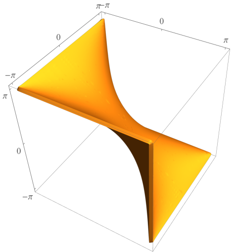
Figure D.2. The secular manifold of the 3-flower. On the left, the secular manifold where $\Sigma_{\mathcal{L}}$ is in blue and $Z_{0}$ is in orange. On the right, only $Z_{0}$ in orange.

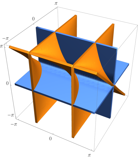
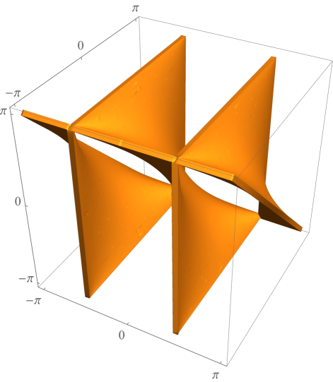
Figure D.3. The secular manifold of the $\left(2,1\right)$-stower. On the left, the secular manifold where $\Sigma_{\mathcal{L}}$ is in blue and $Z_{0}$ is in orange. On the right, only $Z_{0}$ in orange.

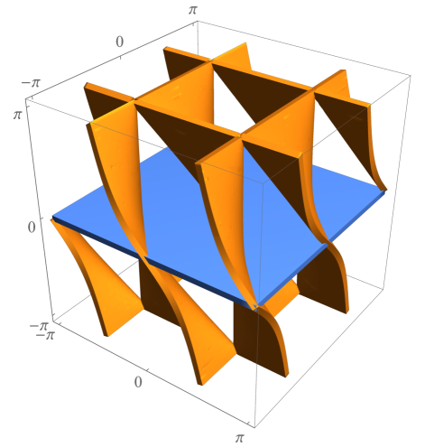
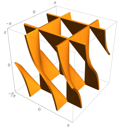
Figure D.4. The secular manifold of the $\left(1,2\right)$-stower. On the left, the secular manifold where $\Sigma_{\mathcal{L}}$ is in blue and $Z_{0}$ is in orange. On the right, only $Z_{0}$ in orange.

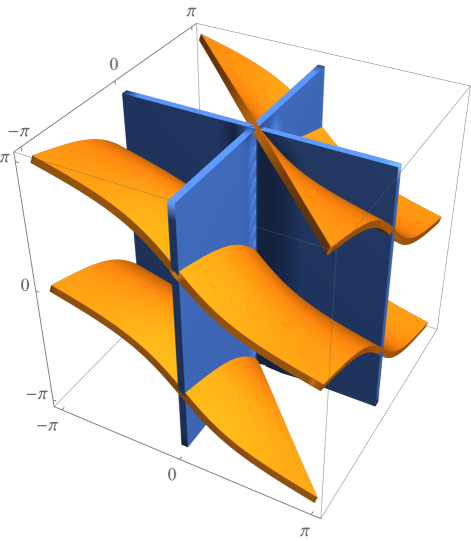
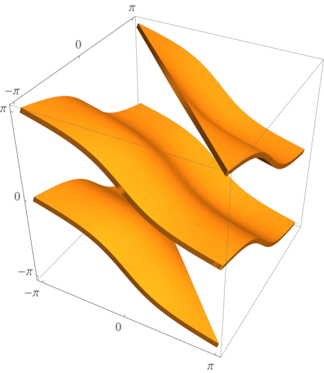
Figure D.5. The secular manifold of the dumbbell graph. On the left, the secular manifold where $\Sigma_{\mathcal{L}}$ is in blue and $Z_{0}$ is in orange. On the right, only $Z_{0}$ in orange.

For graphs e and f which have no loops, we will present the secular manifold $\Sigma$ with $\vec{\kappa}\in\left(0,2\pi\right)^{3}$:

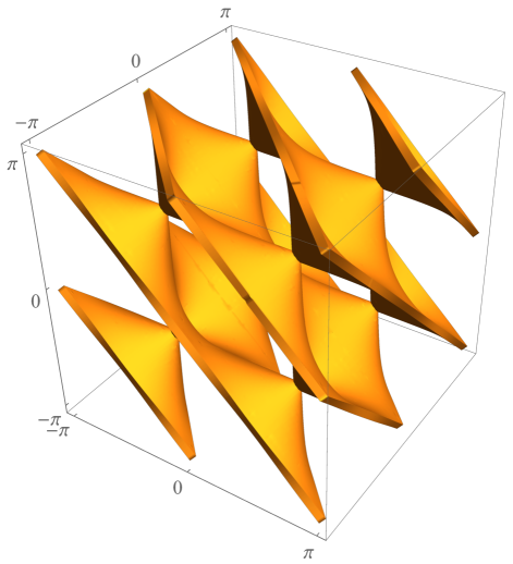
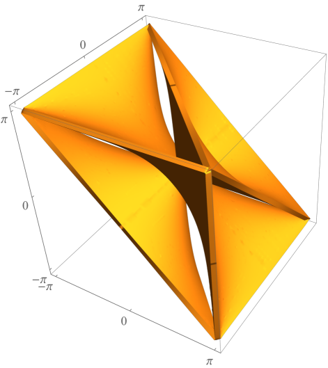
Figure D.6. On the left, the secular manifold of the 3-star graph. On the right, the secular manifold of the 3-mandarin graph.

One may notice that $\Sigma$ of graph f. contains $Z_{0}$ of graph a. In fact, its second sheet is a translation by $\pi$ in each coordinate of $Z_{0}$ of a. It can be explained in terms of the symmetric and antisymmetric eigenfunctions on graph f. [5]

References

- [1] O. Al-Obeid, On the number of the constant sign zones of the eigenfunctions of a dirichlet problem on a network (graph), tech. rep., Voronezh: Voronezh State University, 1992. in Russian, deposited in VINITI 13.04.93, N 938 – B 93. – 8 p.
- [2] J. H. Albert, Topology of the nodal and critical point sets for eigenfunctions of elliptic operators, ProQuest LLC, Ann Arbor, MI, 1972. Thesis (Ph.D.)–Massachusetts Institute of Technology.
- [3] J. H. Albert, Nodal and critical sets for eigenfunctions of elliptic operators, in Partial differential equations (Proc. Sympos. Pure Math., Vol. XXIII, Univ. California, Berkeley, Calif., 1971), Amer. Math. Soc., Providence, R.I., 1973, pp. 71–78.
- [4] S. Alexander, Superconductivity of networks. A percolation approach to the effects of disorder, Phys. Rev. B (3), 27 (1983), pp. 1541–1557.
- [5] L. Alon, Generic eigenfunctions of quantum graphs, In preperation.
- [6] L. Alon and R. Band, Neumann domains on quantum graphs, arXiv:1911.12435, (2019).
- [7] L. Alon, R. Band, and G. Berkolaiko, On a universal limit conjecture for the nodal count statistics of quantum graphs, In preperation.
- [8] L. Alon, R. Band, and G. Berkolaiko, Nodal statistics on quantum graphs, Communications in Mathematical Physics, (2018).
- [9] L. Alon, R. Band, M. Bersudsky, and S. Egger, Neumann domains on graphs and manifolds, Analysis and Geometry on Graphs and Manifolds, 461 (2020), p. 203.
- [10] A. Ancona, B. Helffer, and T. Hoffmann-Ostenhof, Nodal domain theorems à la Courant, Doc. Math., 9 (2004), pp. 283–299 (electronic).
- [11] P. W. Anderson, The question of classical localization. a theory of white paint?, Philosophical Magazine Part B, 52 (1985), pp. 505–509.
- [12] R. Band, The nodal count implies the graph is a tree, Philos. Trans. R. Soc. Lond. A, 372 (2014), pp. 20120504, 24. preprint arXiv:1212.6710.
- [13] R. Band and G. Berkolaiko, Universality of the momentum band density of periodic networks, Phys. Rev. Lett., 111 (2013), p. 130404.
- [14] R. Band, G. Berkolaiko, H. Raz, and U. Smilansky, The number of nodal domains on quantum graphs as a stability index of graph partitions, Commun. Math. Phys., 311 (2012), pp. 815–838.
- [15] R. Band, G. Berkolaiko, and U. Smilansky, Dynamics of nodal points and the nodal count on a family of quantum graphs, Annales Henri Poincare, 13 (2012), pp. 145–184.
- [16] R. Band, S. K. Egger, and A. J. Taylor, The spectral position of neumann domains on the torus, The Journal of Geometric Analysis, (2020), pp. 1–25.
- [17] R. Band and D. Fajman, Topological properties of Neumann domains, Ann. Henri Poincaré, 17 (2016), pp. 2379–2407.
- [18] R. Band and G. Lévy, Quantum graphs which optimize the spectral gap, in Annales Henri Poincaré, vol. 18, Springer, 2017, pp. 3269–3323.
- [19] R. Band, I. Oren, and U. Smilansky, Nodal domains on graphs—how to count them and why?, in Analysis on graphs and its applications, vol. 77 of Proc. Sympos. Pure Math., Amer. Math. Soc., Providence, RI, 2008, pp. 5–27.
- [20] R. Band, O. Parzanchevski, and G. Ben-Shach, The isospectral fruits of representation theory: quantum graphs and drums, J. Phys. A, 42 (2009), pp. 175202, 42.
- [21] R. Band, T. Shapira, and U. Smilansky, Nodal domains on isospectral quantum graphs: the resolution of isospectrality?, J. Phys. A, 39 (2006), pp. 13999–14014.
- [22] R. Band and U. Smilansky, Resolving the isospectrality of the dihedral graphs by counting nodal domains, in Eur. Phys. J. Special Topics, vol. 145, 2007, pp. 171–179.
- [23] F. Barra and P. Gaspard, On the level spacing distribution in quantum graphs, J. Statist. Phys., 101 (2000), pp. 283–319.
- [24] , Transport and dynamics on open quantum graphs, Phys. Rev. E, 65 (2002), p. 016205.
- [25] D. Beliaev and Z. Kereta, On the bogomolny–schmit conjecture, Journal of Physics A: Mathematical and Theoretical, 46 (2013), p. 455003.
- [26] J. v. Below and J. A. Lubary, Isospectral infinite graphs and networks and infinite eigenvalue multiplicities, Netw. Heterog. Media, 4 (2009), pp. 453–468.
- [27] G. Berkolaiko, A lower bound for nodal count on discrete and metric graphs, Comm. Math. Phys., 278 (2008), pp. 803–819.
- [28] , Nodal count of graph eigenfunctions via magnetic perturbation, Anal. PDE, 6 (2013), pp. 1213–1233. preprint arXiv:1110.5373.
- [29] G. Berkolaiko, E. B. Bogomolny, and J. P. Keating, Star graphs and Šeba billiards, J. Phys. A, 34 (2001), pp. 335–350.
- [30] G. Berkolaiko and J. P. Keating, Two-point spectral correlations for star graphs, J. Phys. A, 32 (1999), pp. 7827–7841.
- [31] G. Berkolaiko, J. P. Keating, and U. Smilansky, Quantum ergodicity for graphs related to interval maps, Comm. Math. Phys., 273 (2007), pp. 137–159.
- [32] G. Berkolaiko, J. Kennedy, P. Kurasov, and D. Mugnolo, Surgery principles for the spectral analysis of quantum graphs, Transactions of the American Mathematical Society, 372 (2019), pp. 5153–5197.
- [33] G. Berkolaiko and P. Kuchment, Introduction to Quantum Graphs, vol. 186 of Mathematical Surveys and Monographs, AMS, 2013.
- [34] G. Berkolaiko, P. Kuchment, and U. Smilansky, Critical partitions and nodal deficiency of billiard eigenfunctions, Geom. Funct. Anal., 22 (2012), pp. 1517–1540. preprint arXiv:1107.3489.
- [35] G. Berkolaiko, Y. Latushkin, and S. Sukhtaiev, Limits of quantum graph operators with shrinking edges, Advances in Mathematics, 352 (2019), pp. 632–669.
- [36] G. Berkolaiko and W. Liu, Simplicity of eigenvalues and non-vanishing of eigenfunctions of a quantum graph, J. Math. Anal. Appl., 445 (2017), pp. 803–818. preprint arXiv:1601.06225.
- [37] G. Berkolaiko, H. Raz, and U. Smilansky, Stability of nodal structures in graph eigenfunctions and its relation to the nodal domain count, J. Phys. A, 45 (2012), p. 165203.
- [38] G. Berkolaiko and T. Weyand, Stability of eigenvalues of quantum graphs with respect to magnetic perturbation and the nodal count of the eigenfunctions, in Philosophical Transactions of the Royal Society A’, 2013. arXiv:1212.4475 [math-ph].
- [39] G. Berkolaiko and T. Weyand, Stability of eigenvalues of quantum graphs with respect to magnetic perturbation and the nodal count of the eigenfunctions, Philos. Trans. R. Soc. Lond. Ser. A Math. Phys. Eng. Sci., 372 (2014), pp. 20120522, 17.
- [40] G. Berkolaiko and B. Winn, Relationship between scattering matrix and spectrum of quantum graphs, Trans. Amer. Math. Soc., 362 (2010), pp. 6261–6277.
- [41] M. V. Berry, The bakerian lecture, 1987. quantum chaology, Proceedings of the Royal Society of London. A. Mathematical and Physical Sciences, 413 (1987), pp. 183–198.
- [42] M. V. Berry and M. Tabor, Level clustering in the regular spectrum, Proc. Roy. Soc. Lond. A, 356 (1977), pp. 375–394.
- [43] G. Blum, S. Gnutzmann, and U. Smilansky, Nodal domains statistics: A criterion for quantum chaos, Physical Review Letters, 88 (2002), p. 114101.
- [44] E. Bogomolny and C. Schmit, Percolation Model for Nodal Domains of Chaotic Wave Functions, Physical Review Letters, 88 (2002), p. 114102.
- [45] O. Bohigas, M. J. Giannoni, and C. Schmit, Characterization of chaotic quantum spectra and universality of level fluctuation laws, Phys. Rev. Lett., 52 (1984), pp. 1–4.
- [46] V. Bonnaillie-Noël, B. Helffer, and T. Hoffmann-Ostenhof, Aharonov-Bohm hamiltonians, isospectrality and minimal partitions, Journal of Physics A Mathematical General, 42 (2009), p. 185203.
- [47] J. Bourgain, On Pleijel’s nodal domain theorem, Int. Math. Res. Not. IMRN, (2015), pp. 1601–1612.
- [48] J. Bourgain and Z. Rudnick, On the nodal sets of toral eigenfunctions, Invent. Math., 185 (2011), pp. 199–237.
- [49] J. Brüning, Nodal sets in mathematical physics, The European Physical Journal Special Topics, 145 (2007), pp. 181–189.
- [50] J. Brüning and D. Fajman, On the nodal count for flat tori, Communications in Mathematical Physics, 313 (2012), pp. 791–813.
- [51] J. Brüning, D. Klawonn, and C. Puhle, Comment on ‘resolving isospectral ‘drums’ by counting nodal domains’, Journal of Physics A: Mathematical and Theoretical, 40 (2007), p. 15143.
- [52] V. Cammarota, D. Marinucci, and I. Wigman, On the distribution of the critical values of random spherical harmonics, J. Geom. Anal., 26 (2016), pp. 3252–3324.
- [53] D. Carlson, E. Haynsworth, and T. Markham, A generalization of the schur complement by means of the moore–penrose inverse, SIAM Journal on Applied Mathematics, 26 (1974), pp. 169–175.
- [54] P. Charron, B. Helffer, and T. Hoffmann-Ostenhof, Pleijel’s theorem for schrödinger operators with radial potentials, Annales mathématiques du Québec, 42 (2018), pp. 7–29.
- [55] E. Chladni, Entdeckungen über die Theorie des Klanges, Weidmanns Erben und Reich, Leipzig, 1787.
- [56] Y. Colin de Verdière, Magnetic interpretation of the nodal defect on graphs, Anal. PDE, 6 (2013), pp. 1235–1242. preprint arXiv:1201.1110.
- [57] Y. Colin de Verdière, Semi-classical measures on quantum graphs and the Gauß map of the determinant manifold, Annales Henri Poincaré, 16 (2015), pp. 347–364. also arXiv:1311.5449.
- [58] R. Courant, Ein allgemeiner Satz zur Theorie der Eigenfunktione selbstadjungierter Differentialausdrücke, Nach. Ges. Wiss. Göttingen Math.-Phys. Kl., (1923), pp. 81–84.
- [59] G. F. Dell’Antonio and E. Costa, Effective Schrödinger dynamics on -thin Dirichlet waveguides via quantum graphs: I. Star-shaped graphs, J. Phys. A, 43 (2010), pp. 474014, 23.
- [60] H. Donnelly and C. Fefferman, Nodal sets of eigenfunctions: Riemannian manifolds with boundary, in Analysis, et cetera, Academic Press, Boston, MA, 1990, pp. 251–262.
- [61] H. Edelsbrunner, J. Harer, and Z. A., Hierarchical morse-smale complexes for piecewise linear 2-manifolds, Discrete & Computational Geometry, 30 (2003), pp. 87–107.
- [62] M. Einsiedler and T. Ward, Ergodic theory, Springer, 2013.
- [63] P. Exner and O. Post, Convergence of resonances on thin branched quantum waveguides, J. Math. Phys., 48 (2007), pp. 092104, 43.
- [64] P. Exner and O. Post, Quantum networks modelled by graphs, AIP Conference Proceedings, 998 (2008), pp. 1–17.
- [65] P. Exner and P. Seba, Electrons in semiconductor microstructures: a challenge to operator theorists, in Proceedings of the Workshop on Schrödinger Operators, Standard and Nonstandard (Dubna 1988), World Scientific, Singapore, 1989, pp. 79–100.
- [66] L. Friedlander, Extremal properties of eigenvalues for a metric graph, Ann. Inst. Fourier (Grenoble), 55 (2005), pp. 199–211.
- [67] , Genericity of simple eigenvalues for a metric graph, Israel J. Math., 146 (2005), pp. 149–156.
- [68] Galileo, Discorsi e dimostrazioni matematiche, intorno ‘a due nuove scienze, Louis Elsevier, Leiden, 1638.
- [69] S. Gnutzmann and A. Altland, Spectral correlations of individual quantum graphs, Phys. Rev. E (3), 72 (2005), pp. 056215, 14.
- [70] S. Gnutzmann, P. D. Karageorge, and U. Smilansky, Can one count the shape of a drum?, Phys. Rev. Lett., 97 (2006), pp. 090201, 4.
- [71] S. Gnutzmann and U. Smilansky, Quantum graphs: Applications to quantum chaos and universal spectral statistics, Adv. Phys., 55 (2006), pp. 527–625.
- [72] S. Gnutzmann, U. Smilansky, and N. Sondergaard, Resolving isospectral ‘drums’ by counting nodal domains., J. Phys. A, 38(41) (2005), pp. 8921–8933.
- [73] S. Gnutzmann, U. Smilansky, and J. Weber, Nodal counting on quantum graphs, Waves Random Media, 14 (2004), pp. S61–S73.
- [74] C. Gordon, D. L. Webb, and S. Wolpert, One cannot hear the shape of a drum, Bulletin of the American Mathematical Society, 27 (1992), pp. 134–138.
- [75] B. Gutkin and U. Smilansky, Can one hear the shape of a graph?, J. Phys. A, 34 (2001), pp. 6061–6068.
- [76] M. C. Gutzwiller, Periodic orbits and classical quantization conditions, Journal of Mathematical Physics, 12 (1971), pp. 343–358.
- [77] B. Helffer, Domaines nodaux et partitions spectrales minimales (d’après B. Helffer, T. Hoffmann-Ostenhof et S. Terracini), in Séminaire: Équations aux Dérivées Partielles. 2006–2007, Sémin. Équ. Dériv. Partielles, École Polytech., Palaiseau, 2007, pp. Exp. No. VIII, 23.
- [78] H. Hezari and S. Zelditch, One can hear the shape of ellipses of small eccentricity, arXiv preprint arXiv:1907.03882, (2019).
- [79] J. S. Juul and C. H. Joyner, Isospectral discrete and quantum graphs with the same flip counts and nodal counts, Journal of Physics A: Mathematical and Theoretical, 51 (2018), p. 245101.
- [80] M. Kac, Can one hear the shape of a drum?, The American mathematical monthly, (1966).
- [81] J. P. Keating, Quantum graphs and quantum chaos, in Analysis on graphs and its applications, vol. 77 of Proc. Sympos. Pure Math., Amer. Math. Soc., Providence, RI, 2008, pp. 279–290.
- [82] V. Kostrykin and R. Schrader, Kirchhoff’s rule for quantum wires, J. Phys. A, 32 (1999), pp. 595–630.
- [83] T. Kottos and U. Smilansky, Quantum chaos on graphs, Phys. Rev. Lett., 79 (1997), pp. 4794–4797.
- [84] , Periodic orbit theory and spectral statistics for quantum graphs, Ann. Physics, 274 (1999), pp. 76–124.
- [85] M. Krishnapur, P. Kurlberg, and I. Wigman, Nodal length fluctuations for arithmetic random waves, Annals of Mathematics, (2013), pp. 699–737.
- [86] P. Kuchment, Quantum graphs: an introduction and a brief survey, in Analysis on graphs and its applications, vol. 77 of Proc. Sympos. Pure Math., Amer. Math. Soc., Providence, RI, 2008, pp. 291–312.
- [87] P. Kurasov and M. Nowaczyk, Inverse spectral problem for quantum graphs, J. Phys. A, 38 (2005), pp. 4901–4915.
- [88] , Corrigendum: “Inverse spectral problem for quantum graphs” [J. Phys. A 38 (2005), no. 22, 4901–4915; mr2148632], J. Phys. A, 39 (2006), p. 993.
- [89] P. Kurasov and P. Sarnak, Private communication.
- [90] C. Léna, Pleijel’s nodal domain theorem for neumann and robin eigenfunctions, in Annales de l’Institut Fourier, vol. 69, 2019, pp. 283–301.
- [91] A. Logunov, Nodal sets of laplace eigenfunctions: polynomial upper estimates of the hausdorff measure, Annals of Mathematics, (2018), pp. 221–239.
- [92] A. Logunov and E. Malinnikova, Review of yau’s conjecture on zero sets of laplace eigenfunctions, arXiv preprint arXiv:1908.01639, (2019).
- [93] E. MacCurdy, Notebooks of Leonardo da Vinci, Jonathtan Cape, London, 1938.
- [94] R. B. McDonald and S. A. Fulling, Neumann nodal domains, Philos. Trans. R. Soc. Lond. Ser. A Math. Phys. Eng. Sci., 372 (2014), pp. 20120505, 6.
- [95] J. Milnor, Eigenvalues of the laplace operator on certain manifolds, Proceedings of the National Academy of Sciences, 51 (1964), pp. 542–542.
- [96] B. Mityagin, The zero set of a real analytic function, arXiv:1512.07276, (2015).
- [97] F. Nazarov and M. Sodin, On the number of nodal domains of random spherical harmonics, arXiv:0706.2409v1 [math-ph], (2007).
- [98] F. Nazarov and M. Sodin, Fluctuations in the number of nodal domains, arXiv preprint arXiv:2006.07730, (2020).
- [99] I. Oren, Nodal domain counts and the chromatic number of graphs, J. Phys. A, 40 (2007), pp. 9825–9832.
- [100] I. Oren and R. Band, Isospectral graphs with identical nodal counts, J. Phys. A, 45 (2012), p. 135203. preprint arXiv:1110.0158.
- [101] O. Parzanchevski and R. Band, Linear representations and isospectrality with boundary conditions, J. Geom. Anal., 20 (2010), pp. 439–471.
- [102] L. Pauling, The diamagnetic anisotropy of aromatic molecules, J. Chem. Phys., 4 (1936), pp. 673–677.
- [103] Å. Pleijel, Remarks on Courant’s nodal line theorem, Comm. Pure Appl. Math., 9 (1956), pp. 543–550.
- [104] Y. V. Pokorny, V. L. Pryadiev, and A. Al-Obeid, Oscillation properties of the spectrum of a boundary value problem on a graph, Matematicheskie Zametki, 60 (1996), pp. 468–470.
- [105] Y. V. Pokornyĭ and V. L. Pryadiev, Some problems in the qualitative Sturm-Liouville theory on a spatial network, Uspekhi Mat. Nauk, 59 (2004), pp. 115–150.
- [106] I. Polterovich, Pleijel’s nodal domain theorem for free membranes, vol. 137 of Proc. Amer. Math. Soc., 2009.
- [107] H.-W. Robinson, The diary of robert hooke, 1672-1680, Ciel et Terre, 52 (1936), p. 132.
- [108] J. Rubinstein, Quantum mechanics, superconductivity and fluid flow in narrow networks, in Quantum graphs and their applications, vol. 415 of Contemp. Math., Amer. Math. Soc., Providence, RI, 2006, pp. 251–268.
- [109] R. Rueckriemen and U. Smilansky, Trace formulae for quantum graphs with edge potentials, Journal of Physics A: Mathematical and Theoretical, 45 (2012), p. 475205.
- [110] K. Ruedenberg and C. W. Scherr, Free-electron network model for conjugated systems. i., J. Chem. Phys., 21 (1953), pp. 1565–1581.
- [111] P. Sarnak and I. Wigman, Topologies of nodal sets of random band limited functions, in Advances in the theory of automorphic forms and their -functions, vol. 664 of Contemp. Math., Amer. Math. Soc., Providence, RI, 2016, pp. 351–365.
- [112] P. Schapotschnikow, Eigenvalue and nodal properties on quantum graph trees, Waves in Random and Complex Media, 16 (2006), pp. 167–78.
- [113] E. M. S. Springer Verlag GmbH, Real analytic function. Website. URL: http://encyclopediaofmath.org/index.php?title=Real_analytic_function&oldid=31091.
- [114] S. Steinerberger, A geometric uncertainty principle with an application to Pleijel’s estimate, Ann. Henri Poincaré, 15 (2014), pp. 2299–2319.
- [115] A. Stern, Bemerkungen über asymptotisches Verhalten von Eigenwerten und Eigenfunktionen, 1925.
- [116] C. Sturm, Mémoire sur les équations différentielles linéaires du second ordre, J. Math. Pures Appl., 1 (1836), pp. 106–186.
- [117] T. Sunada, Riemannian coverings and isospectral manifolds, Ann. of Math. (2), 121 (1985), pp. 169–186.
- [118] , Topological crystallography: with a view towards discrete geometric analysis, vol. 6, Springer Science & Business Media, 2012.
- [119] K. Uhlenbeck, Generic properties of eigenfunctions, Amer. J. Math., 98 (1976), pp. 1059–1078.
- [120] D. Ullmo, Bohigas-giannoni-schmit conjecture, Scholarpedia, 11 (2016), p. 31721.
- [121] A. Vogt, Wissenschaftlerinnen in kaiser-wilhelm-instituten: Az, (1999).
- [122] J. von Below, A characteristic equation associated to an eigenvalue problem on -networks, Linear Algebra Appl., 71 (1985), pp. 309–325.
- [123] I. Wigman, On the distribution of the nodal sets of random spherical harmonics, J. Math. Phys., 50 (2009), pp. 013521, 44.
- [124] , Erratum to: Fluctuations of the nodal length of random spherical harmonics [mr2670928], Comm. Math. Phys., 309 (2012), pp. 293–294.
- [125] S. Zelditch, Eigenfunctions and nodal sets, Surveys in Differential Geometry, 18 (2013), pp. 237–308.
- [126] S. Zelditch, Survey on the inverse spectral problem, in Notices of the International Congress of Chinese Mathematicians, vol. 2, International Press of Boston, 2014, pp. 1–20.