Joint Global Fluctuations of complex Wigner and deterministic Matrices

Abstract.

We characterize the limiting fluctuations of traces of several independent Wigner matrices and deterministic matrices under mild conditions. A CLT holds but in general the families are not asymptotically free of second order and the limiting covariance depends on more information on the deterministic matrices than their limiting ^∗-distribution.

1. Introduction

A Wigner matrix is a $N\times N$ Hermitian random matrix of the form $X_{N}=\frac{1}{\sqrt{N}}(x_{ij})$, where:

• the sub-diagonal entries $(x_{ij})_{i\leq j}$ are centered independent complex random variables, (which can also be real-valued, if their imaginary part vanishes identically),

• the diagonal entries are identically distributed real random variables,

• the distribution of $x_{ij}$ does not depend on $N$ and it has bounded moments of all orders ($\mathrm{E}(|x_{ij}|^{k})<\infty$ for all $i,j,k$).

Thanks to the seminal work of Wigner [27], we know that the empirical spectral distribution of a Wigner matrix converges in moments to the semicircular distribution, namely

$$\mathrm{E}\Big{[}\frac{1}{N}\mathrm{Tr}X_{N}^{k}\Big{]}\underset{N\rightarrow\infty}{\longrightarrow}\int_{-2\sigma}^{2\sigma}t^{k}\frac{\sqrt{4\sigma^{2}-t^{2}}}{2\pi\sigma^{2}}\mathrm{d}t,\ \forall k\geq 1,$$

where $\sigma^{2}=\mathrm{E}[|x_{i,j}|^{2}]$ for $i\neq j$. The convergence holds also almost surely and in probability. It also holds in weak-$*$ topology i.e. when integrating the spectral measure with respect to bounded continuous functions instead of polynomials, and in this situation the finite moments condition can be reduced to the existence of a finite second moment. In the multivariate setting this was generalized to the result that independent Wigner matrices and deterministic matrices are asymptotically free, in the sense of Voiculescu’s free probability theory. More precisely, if $\bm{X}$ denotes a collection of independent Wigner matrices and $\bm{A}$ a collection of deterministic matrices, then we have for any ^∗-polynomial $p$

$$\mathrm{E}\Big{[}\frac{1}{N}\mathrm{Tr}\,p(\bm{X},\bm{A})\Big{]}\underset{N\rightarrow\infty}{\longrightarrow}\Phi\big{[}p(\bm{x},\bm{a})\big{]},$$

where $\bm{x}$ denotes a free semicircular system, $\bm{a}$ is distributed according to the limiting ^∗-distribution of $\bm{A}$, and $\bm{x}$ and $\bm{a}$ are free. The case of gue matrices and general deterministic matrices goes back to Voiculescu [25, 26], Dykema [5] considered general Wigner matrices, but special block-diagonal deterministic matrices; the proof of the general case can be found in [1, 18].

The study of fluctuations of linear statistics around their expectation was initiated by Jonsson [10] for the slightly different model of Wishart matrices, and then by Khorunzhy, Khoruzhenko and Pastur [11] for a Wigner matrix. Since then, many more results were produced on the fluctuation of linear spectral statistics of a single random matrix [23, 9, 3, 24, 21, 22]. Our concern in this paper is about the fluctuations of linear statistics in several matrices. This direction of research was initiated by two of the present authors [16], with the study of centered traces of ^∗-polynomials in independent complex Gaussian and Wishart matrices, and has been developed further in [20, 8, 4]. It turns out that in all these situations, one can prove a central limit theorem (CLT) for the centered traces, namely

$$\mathrm{Tr}\,p(\bm{X},\bm{A})-\mathrm{E}\big{[}\mathrm{Tr}\,p(\bm{X},\bm{A})\big{]}$$

converges to a Gaussian random variable, and the convergence holds jointly for all ^∗-polynomials $p$. The absence of normalization is a first remarkable common fact in all these CLT, which tells that the eigenvalues of random matrices fluctuate much less than i.i.d. random variables.

Another aspect that appears in the fluctuation problem, is a breaking of universality compared to the first order problem:

• the limiting fluctuations of linear spectral statistics of a Wigner matrix depend on the pseudo-variance $\mathrm{E}(x_{ij}^{2})$, on the diagonal variance $\mathrm{E}(x_{ii}^{2})$, and on the fourth moment $\mathrm{E}[x_{ij}^{2}\bar{x}_{ij}^{2}]$ of its non diagonal entries.

• the asymptotic second order freeness theory of complex random matrices and of real random matrices are different.

In this article, we extend the result in [16] by considering the fluctuations of traces of several independent Wigner and deterministic matrices, proving a CLT under mild assumptions. It turns out that Wigner matrices and deterministic matrices are, in contrast to gue and deterministic matrices, not free of second order in the sense of [16]. But still there is a very definite structure governing the asymptotic behaviour; however, a crucial observation is that the limiting fluctuations do not depend only on the limiting ^∗-distribution of the deterministic matrices but on more information. This puts this setting very canonically into the frame of traffic probability theory, which was developed by one of present authors [13]. One can see the present investigations as a first step for a more general treatment of global fluctuation by the traffic approach.

The paper is organized as follows. In Section 2, we will present our main results. In the general case, the transpose of the deterministic matrices will also show up in the formula for the asymptotic covariance, thus one needs for the most general version of our results also assumptions on the joint asymptotic distribution of the the deterministic matrices and their transposes. In the special case where the Wigner matrices have vanishing pseudo-variance the transpose does not play a role; hence we will also have a separate discussion for this case. In Sections 3 and 4 we will provide the proofs of our main theorems.

2. Presentation of the results

Assumptions on Wigner and deterministic matrices

Firstly, we list the notations and assumptions on the matrices under consideration.

Hypothesis 1.

Let $X=\frac{1}{\sqrt{N}}({x_{ij}})_{i,j}$ be a Wigner matrix.

1. We assume $\mathrm{E}(|x_{12}|^{2})=1$.

2. We assume $X$ is invariant in law by conjugation by permutation matrices, or equivalently $x_{12}\overset{\mathcal{L}aw}{=}\bar{x}_{12}$.

The first condition is a normalization condition, while the second one is technical and inherent to our proof. We hope that eventually we can get rid of this last one by improving the first steps of our method.

Definition 1.

The triple $(\mathrm{E}(x_{12}^{2}),\mathrm{E}(x_{11}^{2}),k_{4})$ is called the parameters of a Wigner matrix $X=\frac{1}{\sqrt{N}}({x_{ij}})_{i,j}$, where $k_{4}$ is the following fourth cumulant of the off-diagonal entry

$$k_{4}=k_{4}(x_{12},x_{12},\bar{x}_{12},\bar{x}_{12})=\mathrm{E}[x_{12}^{2}\bar{x}_{12}^{2}]-2-|\mathrm{E}[x_{12}^{2}]|^{2}.$$

We call $\mathrm{E}(x_{12}^{2})$ the pseudo-variance and $\mathrm{E}(x_{11}^{2})$ the diagonal variance of the Wigner matrix.

Note that a gue matrix has parameters $(0,1,0)$ and a goe matrix has parameters $(1,2,0)$. A real Wigner matrix has always pseudo-variance equal to one.

Now we introduce the hypotheses on deterministic matrices. These assumptions imply a CLT in the simpler case where the Wigner matrices admit a vanishing pseudo-variance. The general case requires some more assumptions. For two matrices $A$ and $B$, we let $A\circ B$ be the entry-wise product of the matrices, also called Hadamard or Schur product.

Hypothesis 2.

The collection $\bm{A}=(A_{j})_{j\in J}$ of deterministic matrices is assumed to satisfy

1. $\sup_{N}\|A_{j}\|<\infty$ for any $j\in J$, for $\|\,\cdot\,\|$ the operator norm.

2. For any ^∗-polynomials $p$ and $q$,

   $$\varphi_{(\circ)}(p,q):=\varphi(p\circ q):=\underset{N\rightarrow\infty}{\lim}\frac{1}{N}\mathrm{Tr}\big{[}p(\bm{A})\circ q(\bm{A})\big{]}$$

   exists as $N$ goes to infinity.

Definition 2.

Under Hypothesis 2, we call $\varphi_{(\circ)}$ the parameter of $\bm{A}$.

From Hypothesis 2, we have the existence of the limiting $*$-distribution of $\bm{A}$: $\varphi(p)=\varphi(p\circ\mathbb{I})=\varphi(\mathbb{I}\circ p)$, where $\mathbb{I}$ is the unit *-polynomial. Also the first assumption in Hypothesis 2 implies that, up to a subsequence, the second assumption is always satisfied, since $\big{|}\frac{1}{N}\mathrm{Tr}[A\circ B]\big{|}\leq\|A\|\times\|B\|$ for any matrices $A,B$. The limit $\varphi_{(\circ)}$ will be used to describe the covariance of the limiting Gaussian process.

Statements on convergence

Omitting momentarily the description of this covariance, our main result can be stated as follows.

Let us first treat the special case where the Wigner matrices have vanishing pseudo-variance.

Theorem 3.

Let $\bm{X}$ be a collection of independent Wigner matrices, such that each Wigner matrix satisfies Hypothesis 1, and let $\bm{A}$ be a collection of deterministic matrices satisfying Hypothesis 2. In addition assume that all the Wigner matrices of $\bm{X}$ have vanishing pseudo-variance. For any ^∗-polynomial $p$, we denote

$$Z_{N}(p)=\mathrm{Tr}\,p(\bm{X},\bm{A})-\mathrm{E}\big{[}\mathrm{Tr}\,p(\bm{X},\bm{A})\big{]}.$$

Then the process $\big{(}Z_{N}(p)\big{)}_{p}$ converges to a Gaussian process $\big{(}z(p)\big{)}_{p}$. The second order ^∗-distribution

$$\varphi^{(2)}:(p,q)\mapsto\mathrm{E}\big{[}z(p)z(q)\big{]}$$

depends only on the parameters of the matrices as given in Definitions 1 and 2.

Note that the covariance of the process is completely determined by the second-order distribution via the formula $\mathrm{E}\big{[}z(p)\overline{z(q)}\big{]}=\varphi^{(2)}(p,q^{*})$.

We now turn to the case of general Wigner matrices, without any assumption on the pseudo-variance. In this case we also have to control the limit of expressions involving the transpose of the deterministic matrices. We denote by $A^{t}$ the transpose of a matrix $A$.

Theorem 4.

Let $\bm{X}$ be a collection of independent Wigner matrices, such that each Wigner matrix satisfies Hypothesis 1, and let $\bm{A}$ be a collection of deterministic matrices satisfying Hypothesis 2. In addition assume that for any ^∗-polynomials $p$ and $q$, the following limit exists

$$\varphi_{(t)}(p,q):=\varphi(p\,q^{t}):=\underset{N\rightarrow\infty}{\lim}\frac{1}{N}\mathrm{Tr}\big{[}p(\bm{A})q(\bm{A})^{t}\big{]}.$$

Then the conclusion of Theorem 3 is valid, with a limiting second-order ^∗-distribution $\varphi^{(2)}(p,q)$ that also depends on $\varphi_{(t)}$.

Description of the second-order distribution

First, in Theorem 5, we will describe the second-order distribution in the case of vanishing pseudo-variance and unit diagonal variance for all the Wigner matrices (i.e., the parameters for each Wigner matrix are $(0,1,k_{4})$). In Theorem 6 we will then extend this to the general case.

For some $m,n\geq 1$, we consider Wigner matrices $X_{1},\dots,X_{m+n}$ of $\bm{X}$, with possible repetitions of the matrices. Moreover, without loss of generality we assume that the family $\bm{A}$ of deterministic matrices is stable by ^∗-monomials (that is $p(\bm{A})$ is an element of $\bm{A}$ for any ^∗-monomial $p$). We consider deterministic matrices $A_{1},\dots,A_{m+n}$ of $\bm{A}$. Defining the random matrices

$$p_{N}=X_{1}A_{1}\cdots X_{m}A_{m}, q_{N}=X_{m+1}A_{m+1}\cdots X_{m+n}A_{m+n},$$

and the associated polynomials

$$p=x_{1}a_{1}\cdots x_{m}a_{m}, q=x_{m+1}a_{m+1}\cdots x_{m+n}a_{m+n},$$

in order to completely characterize $\varphi^{(2)}$ it is sufficient to give a formula for $\varphi^{(2)}(p,q)$, the limit of

$$\mathrm{E}\big{[}\big{(}\mathrm{Tr}\,p_{N}-\mathrm{E}[\mathrm{Tr}\,p_{N}]\big{)}\big{(}\mathrm{Tr}\,q_{N}-\mathrm{E}[\mathrm{Tr}\,q_{N}]\big{)}\big{]}.$$

Figure 1. The non-crossing annular pairing $\sigma=(1,2)(3,10)\allowbreak(4,5)(6,9)\allowbreak(7,8)\allowbreak(11,12)$. Its Kreweras complement is $K(\sigma)=(1)\allowbreak(\allowbreak 6,\allowbreak 8,2,\allowbreak 10,\allowbreak 12)\allowbreak(3,5,9)(4)(7)(11)$. We have $\varphi_{K(\pi)}(a_{1},\dots,a_{12})=\varphi(a_{1})\allowbreak\varphi(a_{7})\allowbreak\varphi(a_{4})\allowbreak\varphi(a_{6}a_{8}a_{2}a_{10}a_{12})\allowbreak\varphi(a_{3}a_{5}a_{9})\varphi(a_{11})$ and $\widetilde{\varphi}_{K(\pi)}(a_{1},\dots,a_{12})=\varphi(a_{1})\allowbreak\varphi(a_{7})\allowbreak\varphi(a_{4})\allowbreak\varphi(a_{6}a_{8}a_{2}\circ a_{10}a_{12})\allowbreak\varphi(a_{3}a_{5}\circ a_{9})\varphi(a_{11})$.

To give such a formula, we need to recall a few combinatorial facts about annular versions of non-crossing partitions. We refer to [15] for the background definitions on annular non-crossing permutations. We denote by $NC_{2}(m,n)$ the non-crossing pairings on an $(m,n)$-annulus with at least one through string and by $NC_{2}^{(l)}(m,n)$ the non-crossing pairings on an $(m,n)$ annulus with exactly $l$ through strings. We let $\gamma_{m,n}$ be the permutation $(1,2,3,\dots,m)(m+1,\dots,m+n)$ and we put, for a pairing $\sigma\in NC_{2}(m,n)$, $K(\sigma)=\sigma\gamma_{m,n}$; this is a non-crossing permutation called the Kreweras complement of $\sigma$. We define

(1) $$\varphi_{K(\sigma)}(a_{1},\allowbreak\dots,\allowbreak a_{m+n})=\prod_{(i_{1},\dots,i_{\ell})\in K(\sigma)}\varphi(a_{i_{1}}\cdots a_{i_{\ell}}),$$

where the notation means that the product is over the cycles $(i_{1},\dots,\allowbreak i_{\ell})$ of the permutation $K(\sigma)$ (note that, since $K(\sigma)$ is non-crossing, the cycles respect the order on each of the two circles) (see Figure 1) and we recall that $\varphi$ is the limiting ^∗-distribution of the deterministic matrices.

We shall need a modification $\widetilde{\varphi}_{K(\sigma)}$ of $\varphi_{K(\sigma)}$. Let $\sigma\in NC_{2}^{(2)}(m,n)$, then $K(\sigma)$ will have exactly two through cycles. Let us write these through cycles as $(i_{1},\dots,i_{k},i_{k+1},\dots,i_{l})$ and $(j_{1},\dots,j_{k^{\prime}},j_{k^{\prime}+1},\dots,j_{l^{\prime}})$, with $i_{1},\dots,i_{k}\in[m]$ and $i_{k+1},\dots,i_{l}\in[m+1,m+n]$, and $j_{1},\dots,j_{k^{\prime}}\in[m]$ and $j_{k^{\prime}+1},\dots,j_{l^{\prime}}\in[m+1,m+n]$. We define then $\widetilde{\varphi}_{K(\sigma)}(a_{1},\dots,\allowbreak a_{m+n})$ by making the following two replacements in (1):

$$\varphi(a_{i_{1}}\cdots a_{i_{k}}a_{i_{k+1}}\cdots a_{i_{l}}) \mapsto \varphi_{(\circ)}(a_{i_{1}}\cdots a_{i_{k}},a_{i_{k+1}}\cdots a_{i_{l}}),$$

$$\varphi(a_{j_{1}}\cdots a_{j_{k^{\prime}}}a_{j_{k^{\prime}+1}}\cdots a_{j_{l^{\prime}}}) \mapsto \varphi_{(\circ)}(a_{j_{1}}\cdots a_{j_{k^{\prime}}},a_{j_{k^{\prime}+1}}\cdots a_{j_{l^{\prime}}}),$$

where $\varphi_{(\circ)}$ is the bilinear form of Hypothesis 2. This is illustrated in Figure 1.

Theorem 5.

Under the assumption of vanishing pseudo-variance and unit diagonal variance for all involved Wigner matrices, the second-order distribution in Theorem 3 is given by

(2) $$\varphi^{(2)}(p,q)=\\ \kern-10.00002pt\mathop{\sum_{\sigma\in NC_{2}(m,n)}}_{\mathrm{non-mixing}}\kern-10.00002pt\varphi_{K(\sigma)}(a_{1},\dots,a_{m+n})+\kern-10.00002pt\mathop{\sum_{\sigma\in NC_{2}^{(2)}(m,n)}}_{\mathrm{non-mixing}}\kern-10.00002ptk_{4,\sigma}\widetilde{\varphi}_{K(\sigma)}(a_{1},\dots,a_{m+n}).$$

The condition that $\sigma$ is non-mixing means that labels associated to different Wigner matrices belong to different cycles of $\sigma$. In the second sum we also require in addition that the four Wigner matrices involved in the two through cycles must all be the same. The value $k_{4,\sigma}$ is then the parameter of the Wigner matrix corresponding to the two through cycles.

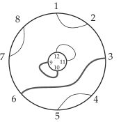
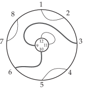
Figure 2. The non-crossing pairing $\sigma=(1,2)(3,6)\allowbreak(4,5)\allowbreak(7,8)\allowbreak(9,10)\allowbreak(11,12)\in NC_{2}(8)\allowbreak\times NC_{2}(4)$. Modifying $(3,6)$ and $(9,10)$, we can produce two elements of $NC_{2}^{(2)}(8,4)$ on the right depending on how we connect the through strings.

Let us now extend our description of the covariance to the general case without any assumption on the the parameters of the Wigner matrices. The second-order distribution is then a slight modification of the function (2) of Theorem 5 that takes into account the pseudo-variance and the diagonal variance parameters. With the same notations as before, consider $\sigma\in NC_{2}^{(\ell)}(m,n)$ with $\ell$ through strings and let $\theta_{\sigma}=\theta_{k_{1}}\cdots\theta_{k_{\ell}}$ be the product of the pseudo-variance parameters of the Wigner matrices $X_{k_{1}},\dots,X_{k_{\ell}}$ associated to the through strings. Without loss of generality, we assume that $\bm{A}$ is closed under the transpose, i.e., if $A\in\bm{A}$, then also $A^{t}\in\bm{A}$. For a monomial $m=x_{1}a_{1}\cdots x_{n}a_{n}$ we denote $s(m)=x_{n}a_{n-1}^{t}x_{n-1}\cdots a_{1}^{t}x_{1}a_{n}^{t}$ and extend this definition of $s$ by linearity. We extend also the definition of $\varphi$ by setting $\varphi(a_{i}a_{j}^{t})=\varphi_{(t)}(a_{i},a_{j})$, of $\varphi_{(\circ)}$ by $\varphi_{(\circ)}(a_{i},a_{j}^{t})=\varphi_{(\circ)}(a_{i},a_{j})$.

Let $\sigma\in NC_{2}^{(1)}(m,n)$, then $K(\sigma)$ will have exactly one through cycle. As before we only have to consider non-mixing $\sigma$, thus the two involved Wigner matrices in the through cycle of $\sigma$ will be the same. We denote by $\eta_{\sigma}$ and $\theta_{\sigma}$ the diagonal variance and the pseudo-variance of this Wigner matrix. We write the through cycle of $K(\sigma)$ as $(i_{1},\dots,i_{k},i_{k+1},\dots,i_{l})$ with $i_{1},\dots,i_{k}\in[m]$ and $i_{k+1},\dots,i_{l}\in[m+1,m+n]$ and define $\widetilde{\varphi}_{K(\sigma)}(a_{1},\dots,a_{m+n})$ by making the following replacement in the factor of $\varphi_{K(\sigma)}(a_{1},\allowbreak\dots,\allowbreak a_{m+n})$ in (1):

$$\varphi(a_{i_{1}}\cdots a_{i_{k}}a_{i_{k+1}}\cdots a_{i_{l}})\mapsto\varphi_{(\circ)}(a_{i_{1}}\cdots a_{i_{k}},a_{i_{k+1}}\cdots a_{i_{l}}).$$

Theorem 6.

For arbitrary parameters $(\theta,\eta,k_{4})$ for each of the involved Wigner matrices, the second-order distribution in Theorem 4 is

$$\varphi^{(2)}(p,q) =\kern-10.00002pt\mathop{\sum_{\sigma\in NC_{2}(m,n)}}_{\mathrm{non-mixing}}\kern-10.00002pt[\varphi_{K(\sigma)}(a_{1},\dots,a_{m+n})+\theta_{\sigma}\cdot(\varphi_{(t)})_{K(\sigma)}(a_{1},\dots,a_{m+n})]$$

(3) $$\quad+\kern-10.00002pt\mathop{\sum_{\sigma\in NC_{2}^{(2)}(m,n)}}_{\mathrm{non-mixing}}\kern-10.00002ptk_{4,\sigma}\cdot\widetilde{\varphi}_{K(\sigma)}(a_{1},\dots,a_{m+n}).$$

$$\quad+\kern-10.00002pt\mathop{\sum_{\sigma\in NC_{2}^{(1)}(m,n)}}_{\mathrm{non-mixing}}\big{(}\eta_{\sigma}-1-\theta_{\sigma}\big{)}\cdot\tilde{\varphi}_{K(\sigma)}(a_{1},\dots,a_{m+n}).$$

Note that the third and the fourth term in Equation (6) cannot appear together. The set $NC_{2}(m,n)$ is only non-empty if $m+n$ is even; if both $m$ and $n$ are even then the number of through cycles of a $\sigma\in NC_{2}(m,n)$ must be even and then $NC_{2}^{(1)}(m,n)$ is empty; if both $m$ and $n$ are odd then the number of through cycles of $\sigma$ must be odd and then $NC_{2}^{(2)}(m,n)$ is empty.

Let us consider some special cases of our Theorem 6.

1. If the pseudo-variance is zero and the diagonal variance is equal to one, then the second and the fourth summand in Equation (6) vanish and the result reduces to Equation (2) of Theorem 5.

2. For gue random matrices, with parameters $(0,1,0)$, only the first summand in Equation (6) is different from zero and reproduces the result for second order freeness between gue and deterministic matrices from [16].

3. For goe random matrices with parameters $(1,2,0)$, the combination $\eta-1-\theta$ is again zero and we have only the first two terms in Equation (6); this yields the formula of Redelmeier [20] for real second order freeness between goe and deterministic matrices.

4. For complex or real Wigner matrices for which the parameters $(\eta,\theta)$ agree with the corresponding Gaussian ensembles, the last term in Equation (6) vanishes and we get in addition to the gue and goe case the term involving $k_{4}$. For the case of trivial deterministic matrices, such results go back to Khorunzhy, Khoruzhenko, and Pastur [11].

Example 7.

1. We have by a direct computation

   $$\varphi^{(2)}(xa_{1},xa_{2}) = \underset{N\rightarrow\infty}{\lim}\mathrm{E}\big{[}\sum_{i,j,i^{\prime},j^{\prime}}A_{1}(i,j)A_{2}(i^{\prime},j^{\prime})X(j,i)X(j^{\prime},i^{\prime})\big{]}$$

   $$= \underset{N\rightarrow\infty}{\lim}\frac{1}{N}\Big{(}\sum_{i\neq j}A_{1}(i,j)A_{2}(j,i)+\sum_{i\neq j}A_{1}(i,j)A_{2}(i,j)\theta$$

   $$+\sum_{i}A_{1}(i,i)A_{2}(i,i)\eta\Big{)}$$

   $$= \underset{N\rightarrow\infty}{\lim}\frac{1}{N}\Big{(}\sum_{i,j}A_{1}(i,j)A_{2}(j,i)+\sum_{i,j}A_{1}(i,j)A_{2}(i,j)\theta$$

   $$+(\eta-1-\theta)\sum_{i}A_{1}(i,i)A_{2}(i,i)\Big{)}$$

   $$= \varphi(a_{1}a_{2})+\varphi(a_{1}a_{2}^{t})+(\eta-1-\theta)\varphi_{(\circ)}(a_{1},a_{2}),$$

   where $\eta$ and $\theta$ are the diagonal variance and pseudo-variance of the Wigner matrix $X$. The three terms indeed correspond to three of the four terms in Theorem 6, since for each term there is a single $\sigma\in NC(1,1)$ which consists in the permutation with a single cycle. Note that the term involving $k_{4}$ does not play a role for this fluctuation of second order, as there is no contributing $\sigma$ with two through cycles.

2. The formula gives for the fluctuation of moments of fourth order

   $$\varphi^{(2)}(x_{\ell_{1}}a_{1}x_{\ell_{2}}a_{2},x_{\ell_{3}}a_{3}x_{\ell_{4}}a_{4})$$

   $$= \Big{(}\delta_{\ell_{1},\ell_{3}}\delta_{\ell_{2},\ell_{4}}\varphi(a_{1}a_{4})\varphi(a_{2}a_{3})+\delta_{\ell_{1},\ell_{4}}\delta_{\ell_{2},\ell_{3}}\varphi(a_{1}a_{3})\varphi(a_{2}a_{4})\Big{)}$$

   $$+\kappa_{4,\ell_{1}}\Big{(}\delta_{\ell_{1},\ell_{2},\ell_{3},\ell_{4}}\varphi_{(\circ)}(a_{1},a_{4})\varphi_{(\circ)}(a_{2},a_{3})+\varphi_{(\circ)}(a_{1},a_{3})\varphi_{(\circ)}(a_{2},a_{4})\Big{)}$$

   $$+\theta_{\ell_{1}}\theta_{\ell_{2}}\Big{(}\delta_{\ell_{1},\ell_{3}}\delta_{\ell_{2},\ell_{4}}\varphi(a_{1}a_{3}^{t})\varphi(a_{2}a_{4}^{t})+\delta_{\ell_{1},\ell_{4}}\delta_{\ell_{2},\ell_{3}}\varphi(a_{1}a_{4}^{t})\varphi(a_{2}a_{3}^{t})\Big{)}.$$

The proofs of Theorems 3-6 are given in the rest of the paper.

3. Boundedness of moments

In the present and the following sections, we consider random matrices $M_{1},\dots,M_{n}$ of the following form: for positive integers $p_{1},\dots,p_{n}$, with $m_{j}=p_{1}+\cdots+p_{j-1}$, $m=m_{n+1}$,

(5) $$\begin{array}[]{cc}M_{j}=X_{m_{j}+1}A_{m_{j}+1}\cdots X_{m_{j}+p_{j}}A_{m_{j}+p_{j}},&\forall j=1,\dots,n,\end{array}$$

where $X_{1},\dots,X_{m}$ are Wigner matrices in $\bm{X}$ and $A_{1},\dots,A_{m}$ are deterministic matrices in $\bm{A}$. As in the previous section, we allow repetitions of matrices. We denote the random variables and the complex numbers

(6) $$Z_{j} = \mathrm{Tr}(M_{j})-\mathrm{E}\big{[}\mathrm{Tr}(M_{j})\big{]},\ \forall\,i=j,\dots,n,$$

(7) $$\tau^{(2)} = \mathrm{E}[Z_{1}\cdots Z_{n}],\ \ \ \tau^{(1)}=\mathrm{E}\Big{[}\prod_{j=1}^{n}\frac{1}{N}\mathrm{Tr}M_{j}\Big{]}.$$

The purpose of this section is to prove that $\tau^{(2)}$ is bounded as $N$ goes to infinity and to give a first combinatorial description of the leading order of $\tau^{(2)}$.

3.1. General scheme for the study of the statistics $\tau^{(1)}$ and $\tau^{(2)}$

Here we summarize the general ideas for the study of the asymptotics of $\tau^{(2)}$ (as well as $\tau^{(1)}$). The basic argument is to translate the computations of moments in terms of a series of graphs.

3.1.1. Preliminary encoding: Labeled graph, quotient graphs and subgraphs

One can check that

(8) $$\tau^{(1)} = \mathrm{E}\Big{[}\prod_{j=1}^{n}\frac{1}{N}\mathrm{Tr}[X_{m_{j}+1}A_{m_{j}+1}\cdots X_{m_{j}+p_{j}}A_{m_{j}+p_{j}}]\Big{]}.$$

This is encoded in terms of a labeled graph $T$ (Definition 8). It consists of a disjoint union $T=T_{1}\sqcup\cdots\sqcup T_{n}$ of $n$ simple directed cycles, where $T_{j}$ has $2p_{j}$ edges with alternating labels $x_{m_{i}+1},a_{m_{i}+1},\dots,x_{m_{i}+p_{1}},a_{m_{i}+p_{i}}$ in the opposite sense of the direction of the cycle, see (a) in Figure 3. Labeled graphs are special cases of the test graphs defined in [13].

Now one can write

(9) $$\tau^{(1)}= N^{-n}\sum_{\bm{i}}\beta^{(1)}_{X}(\bm{i})\times\beta_{A}(\bm{i}),$$

where the sum is over all collections of multi-indices $\bm{i}=\big{(}i_{(j,k)},i_{(j,k)^{\prime}}|j\in[n],k\in[p_{j}]\big{)}$ in $[N]$. Here we have set

(10) $$\quad\beta^{(1)}_{X}\big{(}\bm{i}\big{)} = \prod_{j=1}^{n}\mathrm{E}\big{[}X_{m_{j}+1}(i_{(j,1)},i_{(j,1)^{\prime}})\cdots X_{m_{j}+p_{j}}(i_{(j,p_{j})},i_{(j,p_{j})^{\prime}})\big{]},$$

(11) $$\quad\beta_{A}\big{(}\bm{i}\big{)} = \prod_{j=1}^{n}A_{m_{j}+1}(i_{(j,1)^{\prime}},i_{(j,2)})\cdots A_{m_{j}+p_{j}}(i_{(j,p_{j})^{\prime}},i_{(j,1)}).$$

For any multi-index $\bm{i}$ as above, we denote by $\pi=\ker(\bm{i})$ the partition of the set $V=\{(j,k),(j,k)^{\prime}|j\in[n],k\in[p_{j}]\}$ defined as follows: for $v,w\in V$ we have $v\sim_{\pi}w$ if and only if $i_{v}=i_{w}$. To such a partition $\pi$, one can associate the quotient graph $T^{\pi}$: the labeled graph $T^{\pi}$ is obtained by identifying vertices of $T$ that belong to the same block of $\pi$ (see the general definition in Definition 10).

Now, the invariance by permutation of the Wigner matrices implies that each quantity $\beta^{(1)}_{X}(\bm{i})$ depends only on $\pi=\ker(\bm{i})$. We denote it by $\beta^{(1)}_{X}(\pi)$. We then can write

(12) $$\tau^{(1)}=\sum_{\pi\in\mathcal{P}(V)}N^{-n}\beta^{(1)}_{X}(\pi)\times\beta_{A}(\pi)=:\sum_{\pi\in\mathcal{P}(V)}\alpha^{(1)}(\pi),$$

where the sum is over all partitions of $V$ and

(13) $$\beta_{A}(\pi)=\sum_{\begin{subarray}{c}\bm{i}\in[N]^{V}\\ \ker(\bm{i})=\pi\end{subarray}}\prod_{j=1}^{n}A_{m_{j}+1}(i_{(j,1)^{\prime}},i_{(j,2)})\cdots A_{m_{j}+p_{j}}(i_{(j,p_{j})^{\prime}},i_{(j,1)}).$$

The $\beta$-functions are expressed in terms of subgraphs of $T^{\pi}$. The contribution $\beta_{A}$ of the deterministic matrices is given by (13). Its expression (Definition 13) is written in terms of the subgraph $T_{A}^{\pi}$ of $T^{\pi}$, which has the same vertices as $T^{\pi}$, and has only those edges of $T^{\pi}$ that are labeled by $a_{1},\dots,a_{m}$ (i.e, edges labeled by $x_{k}$ do not appear in $T_{A}^{\pi}$) , see the leftmost graph of (d) in Figure 3. One can similarly define $T_{X}^{\pi}$ (see the rightmost graph (d) in Figure 3). The benefit is that in (12), the sum over $\pi$ is finite (independent of $N$) and we have separated the contributions of the Wigner and the deterministic matrices.

This preliminary encoding is illustrated in Figure 3 below.

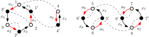
(a) Solid lines: the labeled graph $T=T_{1}\sqcup T_{2}\sqcup T_{3}\sqcup T_{4}$. Dashed lines: a partition with 6 blocks of the vertex set $\pi=\big{\{}\{1,4\},\{1^{\prime},4^{\prime}\},\{2,3^{\prime}\},\{2^{\prime},3\},\allowbreak\{5,6^{\prime},\allowbreak 7,8^{\prime}\},\{5^{\prime},6,7^{\prime},8\}\big{\}}$.

(b) The quotient graph $T^{\pi}$, obtained by identifying the vertices connected by dashed lines.

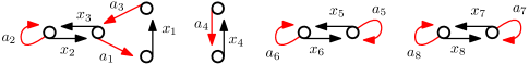
(c) The subgraphs $T^{\pi}_{1},\dots,T^{\pi}_{4}$, obtained by identifying, on each of the subgraphs $T_{1}$, $T_{2}$, $T_{3}$, and $T_{4}$, the vertices connected by dashed lines.

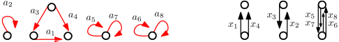
(d) Left: the subgraph $T^{\pi}_{A}$. Right: the subgraph $T_{X}^{\pi}$.

Figure 3. Main graphs used for the proof of main theorems.

The same method can be used to investigate $\tau^{(2)}$. Similarly to Formula (12), one has that

(14) $$\tau^{(2)}=\sum_{\pi\in\mathcal{P}(V)}\alpha^{(2)}(\pi).$$

Each summand $\alpha^{(2)}(\pi)$ is parametrized by the quotient graph $T^{\pi}$, see (b) in Figure 3. Because of the centeredness of the variables appearing in the second-order statistic, the expression of $\beta^{(2)}_{X}(\pi)$ is more convoluted. It is determined by the quotient graphs $T_{j,X}^{\pi}$, $j\in J\subset[1,n]$, for some subset $J$.

3.1.2. Boundedness of the statistics

We can then actually prove the boundedness of

(15) $$\alpha^{(1)}(\pi)=N^{-n}\beta^{(1)}_{X}(\pi)\times\beta_{A}(\pi)$$

for any $\pi$ as $N$ goes to infinity. We mention briefly the next steps for the convergence of $\tau^{(1)}$ (this is valid for any permutation invariant matrices, not just for Wigner matrices).

1. Find appropriate normalizations $\omega^{(1)}_{X}(\pi)=N^{-n_{X}(\pi)}\beta_{X}(\pi)$ and $\omega_{A}(\pi)=N^{-n_{A}(\pi)}\beta_{A}(\pi)$ such that $\omega^{(1)}_{X}$ and $\omega_{A}$ are bounded functions.

2. Prove that whenever $q(\pi):=n_{X}(\pi)+n_{A}(\pi)>n$ then $\omega^{(1)}_{X}(\pi)=0$.

3. Identify the valid partitions $\pi$, i.e., those for which $q(\pi)=n$.

We use the same approach for $\tau^{(2)}$. One can show that the correct normalization of the contribution of the Wigner matrices (Definition 11) is $\omega^{(2)}_{X}(\pi)=N^{\frac{m}{2}}\beta^{(2)}_{X}(\pi)$ (as for $\omega^{(1)}_{X}(\pi)$), where $\beta^{(2)}_{X}(\pi)$ is defined after Eq. (22). Identifying the appropriate normalization of the contribution of the deterministic matrices $\beta_{A}(\pi)$ is more involved. The sharp bounds of [17] imply that the optimal normalization is $\omega_{A}(\pi)=N^{-\frac{\mathfrak{f}(\pi)}{2}}\beta_{A}(\pi)$, where $\mathfrak{f}(\pi)$ is the number of leaves of the forest of two-edge connected components (t.e.c.c.) $\mathcal{T}ec(T^{\pi}_{A})$ of $T_{A}^{\pi}$ (Definition 13). The constant $\mathfrak{f}(\pi)$ may take any integer value greater than or equal to the number of connected components $c(\pi)$ of $T_{A}^{\pi}$. See the two first graphs in Figure 4.

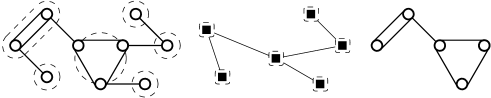
Figure 4. Auxiliary graphs for Section 3. From left to right: a graph $T$ (dashed lines encircle the two-edge connected components of $T$); the tree of two-edge connected components of $\mathcal{T}ec(T)$; the pruning of $\mathcal{P}run(T)$.

From the previous steps, one has that

$$\alpha^{(1)}(\pi)= N^{q(\pi)-n}\omega^{(1)}_{X}(\pi)\omega_{A}(\pi),\quad\alpha^{(2)}(\pi)= N^{q(\pi)}\omega^{(2)}_{X}(\pi)\omega_{A}(\pi),$$

where the $\omega$-functions are bounded and

(16) $$q(\pi)=-\frac{m}{2}+\frac{\mathfrak{f}(\pi)}{2}.$$

Consider a partition $\pi\in\mathcal{P}(V)$, and hence a subgraph $T^{\pi}$, such that the number of leaves $\mathfrak{f}(\pi)$ in the forest of t.e.c.c. of $T^{\pi}_{A}$ equals twice the number of connected components $c(\pi)$ of $T^{\pi}_{A}$, so that $q(\pi)=-\frac{m}{2}+c(\pi)$. One can show that this case gives all the terms contributing to a possible limit of $\tau^{(1)}$ and $\tau^{(2)}$.

To study the quantity $q(\pi)$, we introduce a graph $\mathcal{GDC}(T^{\pi})$ whose topological properties govern the quantity $q(\pi)$. $\mathcal{GDC}(T^{\pi})$ is called the graph of deterministic components of $T^{\pi}$ (Definition 18). It contains $T^{\pi}_{X}$ as a subgraph and is obtained from $T^{\pi}$ by replacing each connected component of $T^{\pi}_{A}$ by a single vertex and by connecting these vertices to $T^{\pi}_{X}$, see (a) in Figure 5. We also denote by $\overline{\mathcal{GDC}}$ the graph obtained from $\mathcal{GDC}(T^{\pi})$ by forgetting the multiplicity of edges. These constructions come from [14, Section 3.7.1] and this step is a particular instance of the asymptotic traffic independence theorem from [13].

(a) The graph of deterministic components $\mathcal{GDC}(T^{\pi})$ of the graph $T^{\pi}$ of Figure 3 (b): the left-most subgraph is of double unicyclic type, the right-most is of 2-4 tree type.

(b) The graph $\overline{\mathcal{GDC}}(T^{\pi})$ obtained by forgetting the edge multiplicity.

Figure 5. Main graphs used for the proof of main theorems.

3.1.3. Asymptotics: Double trees, double unicyclic and 2-4 tree types

In particular, the condition $q(\pi)=n$ implies that the partitions $\pi$ for which $\alpha^{(1)}(T^{\pi})$ contributes in the limit are those such that $T_{X}^{\pi}$ is a forest of double trees, that is a graph whose edges are of multiplicity 2 that becomes a forest when multiplicity is forgotten. This remark is important since double trees (rooted and embedded in the plane) are equivalent to non-crossing pairings, see [7, §1.1.1]. We then obtain

(17) $$\tau^{(1)}=\sum_{\begin{subarray}{c}\pi\in\mathcal{P}(V)\\ q(\pi)=n\end{subarray}}\omega^{(1)}_{X}(\pi)\omega_{A}(\pi)+o(1).$$

For the second-order injective statistic, the centeredness of $Z_{1},\dots,Z_{n}$ and the properties of Wigner matrices imply that $\alpha^{(2)}(\pi)$ tends to zero if at least one connected component $S$ of $T_{X}^{\pi}$ is a double tree. Using the special form of $T$, we will prove that: whenever $\omega^{(2)}_{X}(\pi)\neq 0$ then $q(\pi)\leq 0$. Furthermore one has that $q(\pi)=0$ if and only if each connected component $S$ of $T^{\pi}$ satisfies:

• either the graph of deterministic components $\overline{\mathcal{GDC}}(S)$ of $S$ is a unicyclic graph (removing two edges of $\mathcal{GDC}(S)$ disconnects the graph) and all the edges of $S_{X}$ (associated to Wigner matrices) have multiplicity two (see the leftmost component of $T^{\pi}$ in Figure 3),

• either $\overline{\mathcal{GDC}}(S)$ is a tree (removing one edge disconnects the graph) and all the edges of $S_{X}$ have multiplicity 2 but one which has multiplicity 4 (see the rightmost component of $T^{\pi}$ in Figure 3).

We say that $\pi$ is valid whenever $\overline{\mathcal{GDC}(T^{\pi})}$ satisfies the above properties. The core of the proof will be to show that

(18) $$\tau^{(2)}=\sum_{\begin{subarray}{c}\pi\in\mathcal{P}(V)\\ \mathrm{\ valid}\end{subarray}}\omega^{(2)}_{X}(\pi)\omega_{A}(\pi)+o(1).$$

In order to show (18), one has to consider the case of a partition $\pi$ such that $\mathfrak{f}(\pi)>2c(\pi)$ (such a partition is not valid). The number of additional leaves ${\mathfrak{f}(\pi)}-2c(\pi)$ is then controlled by the number of cycles of $\overline{\mathcal{GDC}}$. Quantitatively, this is measured thanks to the pruning $\tilde{\mathcal{GDC}}(T^{\pi})$ (Definition 29) of the graph of deterministic components. It is obtained by inductively erasing the leaves of $\overline{\mathcal{GDC}}$ until the graph is deleafed, see the rightmost graph in Figure 4. This reasoning allows to prove that if $\mathfrak{f}(\pi)>2c(\pi)$ then $q(\pi)<0$. We can then conclude that the contribution from non-valid partitions vanishes at infinity.

3.2. Expansion in terms of graphs and separation of contributions

We first write $\tau^{(1)}$ and $\tau^{(2)}$ using graph notations. Unless explicitly mentioned, graphs are directed, they can be disconnected, and admit possibly loops and multiple edges. Formally, $V$ is a set and $E$ is a multiset (elements appear with a multiplicity) of elements of $V^{2}$. We consider indeterminates $x_{1},\dots,x_{m},a_{1},\dots,a_{m}$.

Definition 8.

A labeled graph is a triple $T=(V,E,\gamma)$, where $(V,E)$ is a finite graph and $\gamma$ is a labeling map from $E$ to a subset of $\{1,\dots,m\}$.

Below, labeled graphs are given with a partition $E=E_{X}\sqcup E_{A}$ of the edge set. Accordingly an edge $e$ in $E_{X}$ (resp. in $E_{A}$) such that $\gamma(e)=k$ is associated to the indeterminate $x_{k}$ (resp. $a_{k}$). For any $j\in[n]$, we first represent $\mathrm{Tr}\,M_{j}$ by a labeled graph $T_{j}=(V_{j},E_{j},\gamma_{j})$ as follows. The directed graph $(V_{j},E_{j})$ consists of a simple oriented cycle with $2p_{j}$ edges, see (a) in Figure 3: we have $V_{j}=V_{j}^{\circ}\sqcup V_{j}^{\bullet}$, with

$$V_{j}^{\circ}=\{m_{j}+1,\dots,m_{j}+p_{j}\}, V_{j}^{\bullet}=\{(m_{j}+1)^{\prime},\dots,(m_{j}+p_{j})^{\prime}\}.$$

and $E_{j}=E_{j,X}\sqcup E_{j,A}$, with

$$E_{j,X}=\Big{\{}e_{m_{j}+1,x}=\big{(}(m_{j}+1)^{\prime},m_{j}+1\big{)},\dots,\\ e_{m_{j}+p_{j},x}=(m_{j}+p_{j})^{\prime},m_{j}+p_{j})\Big{\}},$$

(representing edges from a vertex of $V_{j}^{\bullet}$ to a vertex of $V_{j}^{\circ}$),

$$E_{j,A}=\Big{\{}e_{m_{j}+1,a}=\big{(}m_{j}+2,(m_{j}+1)^{\prime}\big{)},\dots,\\ e_{m_{j}+p_{j},a}=(m_{j}+1,(m_{j}+p_{j})^{\prime})\Big{\}},$$

(representing edges from a vertex of $V_{j}^{\circ}$ to a vertex of $V_{j}^{\bullet}$). We assign to each edge a label, by means of a map $\gamma_{j}:E_{j}\to\{m_{j}+1,m_{j}+p_{j}\}$ given by $\gamma_{j}(e_{k,x})=\gamma_{j}(e_{k,a})=k$. This indicates that the edge $e_{k,x}$ is associated to the indeterminate $x_{k}$ and $e_{k,a}$ is associated to the indeterminate $a_{k}$.

Definition 9.

1. For any labeled graph $T=(V,E,\gamma)$ and for any map $\psi:V\to[N]$, we denote

   $${r(T,\psi)} = \prod_{\begin{subarray}{c}e\in E_{X}\end{subarray}}X_{\gamma(e)}\big{(}\psi(\mathrm{trg}\ e),\psi(\mathrm{src}\,e)\big{)}$$

   $$\times\prod_{\begin{subarray}{c}e^{\prime}\in E_{A}\end{subarray}}A_{\gamma(e^{\prime})}\big{(}\psi(\mathrm{trg}\,e^{\prime}),\psi(\mathrm{src}\,e^{\prime})\big{)},$$

   with $\mathrm{src}\,e$ and $\mathrm{trg}\,e$ denoting the source and the target, respectively, of the edge $e$.

2. For any labeled graph $T=(V,E,\gamma)$, we denote

   $$\mathrm{Tr}[T]=\sum_{\begin{subarray}{c}\psi:V\to[N]\end{subarray}}r(T,\psi),$$

   and call it the (unnormalized) trace of the labeled graph $T$.

With the above definition we have $\mathrm{Tr}[T_{j}]=\mathrm{Tr}[M_{j}]$, and so

$$\tau^{(1)} := N^{-n}\mathrm{E}\Big{[}\prod_{j=1}^{n}\mathrm{Tr}\,M_{j}\Big{]}=N^{-n}\mathrm{E}\Big{[}\prod_{j=1}^{n}\mathrm{Tr}\,T_{j}\Big{]},$$

$$\tau^{(2)} := \mathrm{E}\bigg{[}\prod_{j=1}^{n}\Big{(}\mathrm{Tr}\,M_{j}-\mathrm{E}\big{[}\mathrm{Tr}\,M_{j}\big{]}\Big{)}\bigg{]}=\mathrm{E}\bigg{[}\prod_{j=1}^{n}\Big{(}\mathrm{Tr}\,T_{j}-\mathrm{E}\big{[}\mathrm{Tr}\,T_{j}\big{]}\Big{)}\bigg{]}.$$

We denote by $T=T_{1}\sqcup\dots\sqcup T_{n}=(V,E,\gamma)$ the labeled graph obtained as the disjoint union of the $n$ graphs. Seeing each $T_{i}$ as a subgraph of $T$, the vertex set $V$ is $V_{1}\sqcup\dots\sqcup V_{n}$, the edge set $E$ is $E_{1}\sqcup\dots\sqcup E_{n}$. Then the map $\gamma:E\to[m]$ is defined by $\gamma(e)=\gamma_{j}(e)$ whenever $e\in E_{j}$.

We can then write $\tau^{(1)}$ and $\tau^{(2)}$ as functions of $T$:

(19) $$\tau^{(1)} = N^{-n}\mathrm{E}\Big{[}\mathrm{Tr}\,T\Big{]}=N^{-n}\sum_{\psi:V\to[N]}\mathrm{E}\Big{[}r(\sqcup_{j\in[n]}T_{j},\psi)\Big{]},$$

(20) $$\tau^{(2)} = \sum_{\psi:V\to[N]}\mathrm{E}\bigg{[}\prod_{j=1}^{n}\Big{(}r(T_{j},\psi_{|V_{j}})-\mathrm{E}\big{[}r(T_{j},\psi_{|V_{j}})\big{]}\Big{)}\bigg{]}.$$

For each $j\in[n]$ we define the subgraph $T_{j,X}=(V_{j},E_{j,X},\gamma_{j,X})$ of $T_{j}$ consisting of the edges $e_{p_{j-1}+1},\dots,e_{p_{j}}$ associated to Wigner matrices. The vertex set of $T_{j,X}$ is still $V_{j}$ and the labelling map $\gamma_{j,X}$ is the restriction of $\gamma_{j}$ to $E_{j,x}$. We also introduce the labeled subgraph $T_{A}=(V,E_{A},\gamma_{A})$ of $T$ consisting of the edges $e_{1}^{\prime},\dots,e_{p_{n}}^{\prime}$. All these labeled graphs consist of disjoint simple edges.

For any map $\psi:V\to[N]$, any $j=1,\dots,n$ and any $J\subset[n]$, we denote by $\psi_{j}$ the restriction of $\psi$ to $V_{j}$ and by $\psi_{J}$ its restriction to $\sqcup_{i\in J}V_{i}$. Since $r(T_{A},\psi)$ is a deterministic quantity, we have

$$\mathrm{E}\Big{[}r(\sqcup_{j\in[n]}T_{j},\psi)\Big{]} = \mathrm{E}\Big{[}r(\sqcup_{j\in[n]}T_{j,X},\psi)\Big{]}\times r(T_{A},\psi)$$

and

$$\mathrm{E}\bigg{[}\prod_{j=1}^{n}\Big{(}r(T_{j},\psi_{j})-\mathrm{E}\big{[}r(T_{j},\psi_{j})\big{]}\Big{)}\bigg{]}$$

$$= \mathrm{E}\Big{[}\prod_{j=1}^{n}\Big{(}r(T_{j,X}\psi_{j})-\mathrm{E}\big{[}r(T_{j,X},\psi_{j})\big{]}\Big{)}\Big{]}\times r(T_{A},\psi)$$

$$= \kern-3.0pt\sum_{J\subset[n]}\mathrm{E}\Big{[}r(\sqcup_{j\in J}T_{j,X},\psi_{J})\Big{]}\times(-1)^{n-|J|}\prod_{j\notin J}\mathrm{E}\Big{[}r(T_{j,X},\psi_{j})\Big{]}\times r(T_{A},\psi).$$

With (19) and (20) this gives a first expression for $\tau^{(1)}$ and $\tau^{(2)}$ where we separate the terms from Wigner and deterministic matrices.

3.3. Regrouping terms and good decomposition

For any map $\psi:V\to[N]$, denote by $\ker\psi$ the partition such that $v\sim_{\ker\psi}w$ whenever $\psi(v)=\psi(w)$, i.e. two vertices are in a same block if and only if $\psi$ attributes the same value for both of them. By permutation invariance of the Wigner matrices, the value of $\mathrm{E}\big{[}r(\sqcup_{j\in J}T_{j,X},\psi_{j})\big{]}$ depends on $\psi$ only through the restriction of $\ker\psi$ on $\sqcup_{j\in J}V_{j}$. For any partition $\pi$ of $V$ and any $J\subset[N]$, we denote by $\pi_{J}$ the restriction of $\pi$ on $\sqcup_{j\in J}V_{j}$ and by $R(\sqcup_{j\in J}T_{j,X},\pi_{J})$ the common value of $\mathrm{E}\big{[}r(\sqcup_{j\in J}T_{j,X},\psi_{J})\big{]}$ for any $\psi$ such that $\ker\psi=\pi$. We then deduce from (19) and (20)

(21) $$\tau^{(1)} = \sum_{\pi\in\mathcal{P}(V)}N^{-n}\beta^{(1)}_{X}(\pi)\times\beta_{A}(\pi),$$

(22) $$\tau^{(2)} = \sum_{\pi\in\mathcal{P}(V)}\beta^{(2)}_{X}(\pi)\times\beta_{A}(\pi),$$

where

$$\beta^{(1)}_{X}(\pi) = R(\sqcup_{j\in[n]}T_{j,X},\pi),\>\beta_{A}(\pi)=\sum_{\begin{subarray}{c}\psi:V\to[N]\\ \mathrm{s.t.\,}\ker\psi=\pi\end{subarray}}r(T_{A},\psi),$$

$$\beta^{(2)}_{X}(\pi) = \sum_{J\subset[n]}(-1)^{n-|J|}R(\sqcup_{j\in J}T_{j,X},\pi_{J})\times\prod_{j\notin J}R(T_{j,X},\pi_{j}).$$

3.3.1. Contribution from Wigner matrices

By the definition of the function $R$ and due to the $\frac{1}{\sqrt{N}}$-normalization of Wigner matrices, it is clear that $\omega^{(i)}_{X}(\pi):=N^{\frac{m}{2}}\beta^{(i)}_{X}(\pi)$ is bounded. We re-write below this contribution in an explicit way.

Definition 10.

For any labeled graph $S=(W,F,\delta)$ and any partition $\pi$ of $W$, we define by $S^{\pi}=(W^{\pi},F^{\pi},\delta^{\pi})$ the labeled graph obtained by identifying vertices of $S$ that belong to a same block of $\pi$. An edge $e=(v,w)$ of $S$ becomes an edge $e_{\pi}=(B_{v},B_{w})$ of $S^{\pi}$, where $B_{v}$ and $B_{w}$ are respectively the blocks containing $v$ and $w$. The label of $e_{\pi}$ is the label of $e$, namely $\delta^{\pi}(e_{\pi})=\delta(e)$. We say that $S^{\pi}$ is a quotient of $S$.

Note that for $j=1,\dots,n$ and any $\pi\in\mathcal{P}(V_{j})$ one has $R(T_{j,X},\pi)=R(T_{j,X}^{\pi},\bm{0})$, where $\bm{0}$ is the partition consisting of singletons only.

Definition 11.

Let $T^{\pi}$ be a quotient graph of $T=T_{1}\sqcup\cdots\sqcup T_{n}$. Denote by $T_{j}^{\pi}=(V^{\pi}_{j},E^{\pi}_{j},\gamma^{\pi}_{j})$ the quotient of $T_{j}$ by $\pi$ for any $j\in[n]$. We define the weights associated to the Wigner matrices by

$$\omega^{(1)}_{X}(\pi) = \mathrm{E}\Big{[}\prod_{\begin{subarray}{c}e\in E^{\pi}_{j,x}\\ \forall j\in[n]\end{subarray}}\sqrt{N}X_{\gamma_{j}^{\pi}(e)}\big{(}\psi_{0}(\mathrm{trg}\,e),\psi_{0}(\mathrm{src}\,e)\big{)}\Big{]}$$

(23) $$\omega^{(2)}_{X}(\pi) = \sum_{J\subset[n]}\mathrm{E}\Big{[}\prod_{\begin{subarray}{c}e\in E^{\pi}_{j,x}\\ \forall j\in J\end{subarray}}\sqrt{N}X_{\gamma_{j}^{\pi}(e)}\big{(}\psi_{0}(\mathrm{trg}\,e),\psi_{0}(\mathrm{src}\,e)\big{)}\Big{]}$$

$$\ \ \ \times(-1)^{n-|J|}\prod_{j\notin J}\mathrm{E}\Big{[}\prod_{e\in E^{\pi}_{j,x}}\sqrt{N}X_{\gamma^{\pi}_{j}(e)}\big{(}\psi_{0}(\mathrm{trg}\,e),\psi_{0}(\mathrm{src}\,e)\big{)}\Big{]},$$

for any choice of injective map $\psi_{0}:V_{j}\to[N]$ (the value is independent of this choice).

Example 12.

Let $n=4$ and $T$ and $\pi$ be as Figure 3. We denote by $z_{j}$ a random variable distributed as the $(1,2)$ entry of the (unnormalized) Wigner matrix $\sqrt{N}X_{j}$. For any $J\subset[n]$ we denote by $\omega_{X}(\pi)[J]$ the corresponding summand in Equation (23). For $J=\{1,2,3,4\}$, we have

$$\omega_{X}(\pi)[J]=\mathrm{E}[z_{2}\overline{z_{3}}]\mathrm{E}[z_{1}z_{4}]\mathrm{E}[z_{5}z_{7}\overline{z_{6}z_{8}}].$$

We recall that when denoting the Wigner matrices $X_{1},\dots,X_{m}$ we allow possible repetition of a same matrix, and so this term is possibly nonzero only when $X_{2}=X_{3}$, $X_{1}=X_{4}$, and some repetitions occur among the matrices $X_{5},\dots,X_{8}$. Note also that we can indifferently write $\mathrm{E}[z_{3}\overline{z_{2}}]$ instead of $\mathrm{E}[z_{2}\overline{z_{3}}]$ since these quantities are equal by complex conjugate invariance of Wigner matrices entries. For $J=\{1,2\},\{1,2,3\},\{1,2,4\}$, we have in each case

$$\omega_{X}(\pi)[J]=\mathrm{E}[z_{2}\overline{z_{3}}]\mathrm{E}[z_{1}z_{4}]\mathrm{E}[z_{5}\overline{z_{6}}]\mathrm{E}[z_{7}\overline{z_{8}}].$$

Otherwise, when $J$ does not contain both $1$ and $2$, then

$$\omega_{X}(\pi)[J]=\mathrm{E}[z_{2}\overline{z_{3}}]\mathrm{E}[z_{1}]\mathrm{E}[z_{4}]\times\dots=0$$

by centeredness of the entries.

3.3.2. Contribution from deterministic matrices

Definition 13.

For any labeled graph $S$ with vertex set $W$, the (unnormalized) injective trace of the labeled graph $S$ is

$$\mathrm{Tr}^{0}[S]=\sum_{\begin{subarray}{c}\psi:W\to[N]\\ \mathrm{injective}\end{subarray}}r(S,\psi),$$

where $r(S,\psi)$ is defined in Definition 9.

We also need the following definition.

Definition 14.

1. A cutting edge of a graph is an edge whose removal increases the number of connected components.

2. A two-edge connected graph is a connected graph with no cutting edge. Similarly a two-edge connected component of a graph is a maximal connected sub-graph which is two-edge connected.

3. The forest of two-edge connected components of a graph $S$ is the graph $\mathcal{T}ec(S)$ whose vertices are the two-edge connected components of $S$ and whose edges are the cutting edges of $S$, making links between the components that contain the source and the target of the edge.

4. A trivial component of $\mathcal{T}ec(S)$ is a component consisting of a single vertex. We denote by $\mathfrak{f}(S)$ the number of leaves of the forest of two-edge connected components $\mathcal{T}ec(S)$, with the convention that a trivial component has two leaves.

Lastly we define the weight associated to the deterministic matrices.

Definition 15.

Let $\pi$ be a partition of the vertices of $T$. We define the weight $\omega_{A}(\pi)$ associated to the deterministic matrices by

(24) $$\omega_{A}(\pi) = {N^{-\frac{\mathfrak{f}(T^{\pi}_{A})}{2}}}\mathrm{Tr}^{0}\big{[}T^{\pi}_{A}\big{]}.$$

Example 16.

Let $T$ and $\pi$ be as Figure 3. The leftmost graph $T_{A}^{\pi}$ of (d) in Figure 3 has 4 connected components, all of them are two edge-connected. Hence by convention one has that $\frac{\mathfrak{f}(T^{\pi}_{A})}{2}=4$. Then one has

$$\omega_{A}(\pi) = N^{-4}\sum_{\begin{subarray}{c}i_{1},\dots,i_{8}\in[N]\\ \mathrm{pairwise\ distinct}\end{subarray}}A_{2}(i_{1},i_{1})\times A_{1}(i_{2},i_{3})A_{3}(i_{3},i_{4})A_{4}(i_{2},i_{4})$$

$$\ \ \ \times A_{5}(i_{5},i_{5})A_{7}(i_{5},i_{5})\times A_{6}(i_{6},i_{6})A_{8}(i_{6},i_{6})$$

Lemma 17.

For any $\pi\in\mathcal{P}(V)$, $\omega_{A}(\pi)$ is bounded uniformly in $N$.

Proof.

We have the relation

$$\mathrm{Tr}^{0}[T_{A}^{\pi}]=\sum_{\pi^{\prime}\in\mathcal{P}(V^{\pi})}\mathrm{Mob}(0,\pi^{\prime})\mathrm{Tr}[T_{A}^{\pi^{\prime}}],$$

where $\mathrm{Mob}$ is the Möbius function of the poset of partitions of the vertex set of $T_{A}^{\pi}$, see [13]. By [17], for any labeled graph $T_{A}^{\pi^{\prime}}$ we have the bound

$$\big{|}\mathrm{Tr}[T_{A}^{\pi^{\prime}}]\big{|}\leq N^{\frac{\mathfrak{f}(T_{A}^{\pi^{\prime}})}{2}}\times\prod_{j=1}^{n}\|A_{j}\|.$$

Note moreover that $\mathfrak{f}(T_{A}^{\pi})\geq\mathfrak{f}(T_{A}^{\pi^{\prime}})$ for any $\pi^{\prime}\in\mathcal{P}(V^{\pi})$, i.e. the number of leaves of the forest of two-edge connected components cannot increase by taking a quotient. Hence $\mathrm{Tr}[T_{A}^{\pi^{\prime}}]=O\big{(}N^{\frac{\mathfrak{f}(T_{A}^{\pi})}{2}}\big{)}$ for any $\pi^{\prime}\in\mathcal{P}(V^{\pi})$, and so we get as well $\mathrm{Tr}^{0}[T_{A}^{\pi}]=O\big{(}N^{\frac{\mathfrak{f}(T_{A}^{\pi})}{2}}\big{)}$. The proof then follows from (24). ∎

Recalling from Eq. (16) that $q(\pi)=-\frac{m}{2}+\frac{\mathfrak{f}(T_{A}^{\pi})}{2}$, we have finally obtained

(25) $$\tau^{(1)} = \sum_{\pi\in\mathcal{P}(V)}N^{q(\pi)-n}\omega^{(1)}_{X}(\pi)\times\omega_{A}(\pi),$$

(26) $$\tau^{(2)} = \sum_{\pi\in\mathcal{P}(V)}N^{q(\pi)}\omega^{(2)}_{X}(\pi)\times\omega_{A}(\pi),$$

where we recall that $\omega^{(1)}_{X}$ and $\omega^{(2)}_{X}$ are defined in (23), $\omega_{A}$ is defined in (24). Note that $m$ equals $|E_{X}|$ the total number of edges associated to Wigner matrices in $T$ (or equivalently in $T^{\pi}$).

3.4. The topological analysis

In this subsection we identify the partitions that contribute to $\tau^{(1)}$ and $\tau^{(2)}$. To describe the connected components that contribute to the limit of these statistics, we need the following Definitions 18 and 21.

Fix $\pi$ in $\mathcal{P}(V)$ and denote by $V^{\pi}$ the vertex set of $T^{\pi}$ and $E^{\pi}$ its multi-set of edges. We first analyze in more detail the quantity $q(\pi)$.

Definition 18.

The graph of deterministic components of $T^{\pi}$ is the undirected graph $\mathcal{GDC}(T^{\pi})=(\mathcal{V},\mathcal{E})$, where

• the vertex set $\mathcal{V}$ consists of the disjoint union of the vertex set $V^{\pi}$ of $T_{X}^{\pi}$ and of the set $C_{A}$ of connected components of $T^{\pi}_{A}$ (we will in the following call the elements of $C_{A}$ as deterministic components),

• the edge set $\mathcal{E}$ consists of the disjoint union of $E^{\pi}_{X}$ (i.e. the set of edges of $T_{X}^{\pi}$) and of the set of pairs $(v,C)$, $v\in V^{\pi}$, $C\in C_{A}$ such that $v\in C$ in the graph $T^{\pi}$.

We also denote $\overline{\mathcal{GDC}}(T^{\pi})(\mathcal{V},\overline{\mathcal{E}})$ the graph obtained from $\mathcal{GDC}(T)$ by forgetting the multiplicity of its edges, and assuming that this multiplicity is one for each edge.

See examples (e) and (f) in Figure 3. When the quotient graph $T^{\pi}$ is fixed without ambiguity, we write $\mathcal{GDC}$ as a shortcut for $\mathcal{GDC}(T^{\pi})$. By definition, the number of vertices of ${\mathcal{GDC}}$ is $|\mathcal{V}|=|V^{\pi}|+|C_{A}|$. Denote by $|\overline{E^{\pi}_{X}}|$ the number of edges of $T^{\pi}_{X}$ counted without multiplicity. We see that the number of edges without counting multiplicity is $|\overline{\mathcal{E}}|=|\overline{E^{\pi}_{X}}|+|V^{\pi}|$, since each vertex $v$ of $T^{\pi}$ is connected exactly to one deterministic component. We then write

(27) $$q(\pi) = -\frac{|E_{X}|}{2}+\frac{\mathfrak{f}(T^{\pi}_{A})}{2}$$

$$= \underbrace{\big{(}|\overline{E^{\pi}_{X}}|-\frac{|E_{X}|}{2}\big{)}}_{:=q_{1}}+\underbrace{\big{(}|\mathcal{V}|-|\bar{\mathcal{E}}|\big{)}}_{:=q_{2}}+\underbrace{\Big{(}\frac{\mathfrak{f}(T^{\pi}_{A})}{2}-|C_{A}|\Big{)}}_{:=q_{2}^{\prime}}.$$

Note that $q_{1}$ and $q_{2}^{\prime}$ are half integers, whereas $q_{2}$ is an integer. All the quantities involved are implicitly functions of $\pi$, and are additive with respect to the different connected components $\mathcal{GDC}_{i}$, $i=1,\dots,c$, of $\mathcal{GDC}$. We denote, for each $i=1,\dots,c$, by $q_{1,i}$, $q_{2,i}$, and $q_{2,i}^{\prime}$ the version of $q_{1}$, $q_{2}$, and $q_{2}^{\prime}$, respectively, defined for the $i$-th component $\mathcal{GDC}_{i}$.

We here state two lemmas that we use in the rest of the section.

Lemma 19.

Let $\mathcal{G}=(\mathcal{V},\mathcal{E})$ be a finite connected graph. Then $|\mathcal{V}|-|\mathcal{E}|\leq 1$ with equality if and only if $\mathcal{G}$ is a tree.

The second one is referred to as a parity argument.

Lemma 20.

Let $S$ be the quotient of a union of simple cycles. Let $\bar{e}$ be a group of twin edges in $S$. If the removal of the edges of $\bar{e}$ disconnects the graph $S$, then the multiplicity of the edges of $S$ coming from each cycle is an even number, with an equal number of edges in one direction and in the other direction.

Proof.

Assume that a cycle $C$ has $m\geq 1$ twin edges in the group of edges associated to $\bar{e}$. We show the lemma by induction on $m$.

We first prove that necessarily $m>1$. Assume, for a contradiction, that $C$ has a one single edge $e_{0}$ that represents $\bar{e}$. Let $C\setminus{e_{0}}$ be the graph obtained from $C$ by removing $e_{0}$. Since $C$ is a cycle, $C\setminus{e_{0}}$ is connected, and so in every quotient of $C\setminus{e_{0}}$ the image of the source and target of $e_{0}$ belong to a same connected component. Let $S\setminus{\bar{e}}$ denote the graph obtained from $S$ by removing all the edges representing $\bar{e}$. Since in $S\setminus{\bar{e}}$ there is a subgraph which is a quotient of $C\setminus{e_{0}}$, then the source and target of the edge of $\bar{e}$ belong to a same connected component. But this is in contradiction with the assumption that the removal of $\bar{e}$ disconnects $S$. Hence the multiplicity $m$ is at least equal to 2.

We now assume that $m$ is larger than 2. We consider a closed walk on $S$, given by the image of the cycle $C$ and starting at an edge $e_{0}$ in $C$ representing $\bar{e}$. Let $e_{1}$ be the edge of $C$ that is the first representant of $\bar{e}$ that the walk meets after $e_{0}$. Necessarily in the quotient graph, the source of $e_{0}$ is the target of $e_{1}$ and vice versa: indeed, otherwise one sees (as in the previous paragraph) that removing the edges of $\bar{e}$ in $S$ would not disconnect the graph. We now denote by $C^{\prime}$ the graph obtained from $C$ by identifying the source of $e_{0}$ with the target of $e_{1}$, and deleting $e_{0},e_{1}$, all the edges inbetween them and all vertices that stay isolated after this process. Hence $C^{\prime}$ is a simple cycle such that of smaller size and has $m-2$ edges representing $e$. By induction, $C$ has an equal number of edges representing $\bar{e}$ in both directions, which concludes the proof of Lemma 20. ∎

We can now state the main result of this subsection, thanks to the following definition.

Definition 21.

• The $i$-th component of $T^{\pi}$ is of double tree type whenever $(q_{1,i},q_{2,i})=(0,1)$, which means that the edges of $\mathcal{GDC}_{i}$ associated to Wigner matrices have multiplicity two and that $\overline{\mathcal{GDC}}_{i}$ is a tree.

• The $i$-th component of $T^{\pi}$ is of double unicyclic type whenever $(q_{1,i},q_{2,i})=(0,0)$, which means that the edges of $\mathcal{GDC}_{i}$ associated to Wigner matrices have multiplicity two and that $\overline{\mathcal{GDC}}_{i}$ is a graph with a unique simple cycle.

• The $i$-th component of $T^{\pi}$ is of 2-4 tree type whenever $(q_{1,i},q_{2,i})\allowbreak=(-1,1)$, which means that $\overline{\mathcal{GDC}}_{i}$ is a tree and that the edges of $\mathcal{GDC}_{i}$ associated to Wigner matrices have multiplicity two, except for one group of edges of multiplicity four.

We denote by $\mathcal{D}\mathcal{T}_{c}$ the set of partitions $\pi$ of $V$ such that $T^{\pi}$ has $c\in[n]$ connected components and all are of double tree type. We denote by ${\mathcal{DU}}\&{\mathcal{FT}}$ the set of partitions such that the components are either of double unicyclic or 2-4 tree type.

Here is now the main result in our analysis of the $\tau$-functions, which computes the leading order in their asymptotic expansion. Recall that $n$ is the number of connected components of $T$.

Proposition 22.

One has the asymptotic large $N$ expansion

(28) $$\tau^{(1)}=\sum_{\pi\in\mathcal{D}\mathcal{T}_{n}}\omega^{(1)}_{X}(\pi)\times\omega_{A}(\pi)+o(1),$$

(29) $$\tau^{(2)}=\sum_{\pi\in{\mathcal{DU}}\&{\mathcal{FT}}}\omega^{(2)}_{X}(\pi)\times\omega_{A}(\pi)+o(1).$$

Remark 1.

The asymptotics for $\tau_{1}$ are the same as in the Gaussian case. The first statement is thus a universality statement.

The proof of Proposition 22 relies on the following two lemmas, where we recall that the notations for $q(\pi)=q_{1}+q_{2}+q_{2}^{\prime}$ is from (27).

Lemma 23.

Let $\pi\in\mathcal{P}(V)$ and denote by $c=c(\pi)$ the number of connected components of $T^{\pi}$. If $\omega_{X}^{(1)}\neq 0$, then $q_{1}+q_{2}\leq c$ with equality if and only if $\pi\in{\mathcal{DT}}_{c}$. Moreover if $\omega_{X}^{(2)}\neq 0$ then $q_{2,i}+q^{\prime}_{2,i}\leq 0$ with equality if and only if $\pi\in{\mathcal{DU}}\&{\mathcal{FT}}$.

The quantity $q^{\prime}_{2,i}$ is taken under consideration in the next Lemma.

Lemma 24.

1. If the multiplicity in the $i$-th component of $T^{\pi}$ of edges labeled by Wigner matrices is even, then $q_{2,i}^{\prime}=0$.

2. If $q_{2,i}\leq 0$, i.e. $\overline{\mathcal{GDC}}_{i}$ is not a tree, then $q_{2,i}+q_{2,i}^{\prime}\leq 0$.

Proof of Proposition 22.

Assume that Lemmas 23 and 24 hold true and let $\pi\in\mathcal{P}(V)$.

Assume that $\omega^{(1)}_{X}(\pi)\neq 0$. Then one has that $q_{1,i}\leq 0$. Either $\overline{\mathcal{GDC}}_{i}$ is a tree, and the parity argument (Lemma 20) implies that the number of edges labeled by Wigner matrices is even; so the first parts of the lemmas imply $q(\pi)-n=q_{1}+q_{2}+q_{2}^{\prime}-n=q_{1}+q_{2}-n\leq 0$ with equality only if $\pi\in{\mathcal{DT}}_{n}$. Either $\overline{\mathcal{GDC}}_{i}$ is not a tree, and the second part of Lemma 24 implies $q_{i}(\pi)-1=q_{1,i}+q_{2,i}+q^{\prime}_{2,i}-1\leq q_{1,i}-1\leq-1$. Hence in (25) the only $\pi$ that contribute for $\tau^{(1)}$ in the limit are those such that $T^{\pi}\in{\mathcal{DT}}_{n}$, which proves of (28).

Assume now that $\omega^{(2)}_{X}(\pi)\neq 0$. If $\overline{\mathcal{GDC}}_{i}$ is a tree, the parity argument and the first part of Lemma 24 imply again $q_{2,i}^{\prime}=0$, and the second part of Lemma 23 implies that $q_{i}(\pi)=q_{1,i}+q_{2,i}+0\leq 0$ with equality whenever the $i$-th component of $T^{\pi}$ is of 2-4 tree type. Assume now $\overline{\mathcal{GCD}_{i}}$ is not a tree, i.e. $q_{2,i}\leq 0$. By the second part of Lemma 24, one has that $q_{i}(\pi)=q_{1,i}+q_{2,i}+q_{2,i}^{\prime}\leq 0$. If $q_{i}(\pi)=0$, the multiplicity of edges labeled by Wigner matrices is 2. The first part of Lemma 24 hence implies that $q_{2,i}^{\prime}=0$. Hence, when $\mathcal{GCD}_{i}$ is not a tree, $q_{i}(\pi)=0$ if and only if the $i$-th component is of double unicyclic type. We thus have shown that the partitions $\pi$ that contribute to $\tau^{(2)}$ in (26) are those such that $\pi\in{\mathcal{DU}}\&{\mathcal{FT}}$, which proves (29) and concludes the proof of Lemma 22. ∎

3.4.1. Proof of Lemma 23

We turn to the proof of Lemma 23.

The first function $q_{1}$ is a linear combination of the numbers of edges of $T^{\pi}$ labeled $X$ when counting and not counting the multiplicity. If $T^{\pi}$ has an edge of multiplicity one then for any $J\subset[n]$ so has either $\sqcup_{j\in J}T^{\pi}_{J}$ or one of the $T^{\pi}_{j}$, $j\notin J$; hence by independence and centeredness of the entries of Wigner matrices, and by Formula (23) we get $\omega_{X}^{(1)}(\pi)=\omega_{X}^{(2)}(\pi)=0$. So we can assume that the multiplicity of each edge of $T^{\pi}$ labeled by a Wigner matrix is at least 2 and we can restrict to $\pi$ with $q_{1}\leq 0.$

Lemma 19 applied component-wise implies $q_{2,i}\leq 1$ for any $i=1,\dots,c$ with equality whenever $\overline{\mathcal{GDC}_{i}}$ is a tree. Assuming there is no edge of multiplicity one in $T^{\pi}_{X}$, the possible maximal order of $N^{q_{1,i}+q_{2,i}}$ given by the $i$-th connected component of $T^{\pi}$ is $N$ when $q_{1,i}=0$ and $q_{2,i}=1$. This means that the edges of $\mathcal{GDC}_{i}$ associated to Wigner matrices have multiplicity two and that $\overline{\mathcal{GDC}}_{i}$ is a tree, i.e. the components of $T^{\pi}$ are of double tree type.

We have proved the first part of Lemma 23: when $\omega^{(1)}_{X}(\pi)\neq 0$ (and in particular $q_{1}\leq 0$) then $q_{1}+q_{2}\leq c$ with equality whenever $\pi\in{\mathcal{DT}}_{c}$.

For the second part of the lemma, we use further arguments. We define below the property of $X$-connectedness. Recall that $T^{\pi}_{j}$, $j=1,\dots,n$, denote the quotients of the cycles forming $T$, that we see as subgraphs of $T^{\pi}$.

Definition 25.

• We say that two edges $e$ and $e^{\prime}$ of $T_{X}^{\pi}$ are twin in $\mathcal{GDC}(T^{\pi})$ whenever they share the same pair of vertices: $\mathrm{trg}\ e=\mathrm{trg}\ e^{\prime}$ and $\mathrm{src}\ e=\mathrm{src}\ e^{\prime}$, or $\mathrm{trg}\ e=\mathrm{src}\ e^{\prime}$ and $\mathrm{src}\ e=\mathrm{trg}\ e^{\prime}$.

• We say that two graphs $T^{\pi}_{j}$ and $T^{\pi}_{j^{\prime}}$ are $X$-connected whenever there is an edge $e$ of $T^{\pi}_{j}$ and an edge $e^{\prime}$ of $T^{\pi}_{j^{\prime}}$ that are twin and associated to Wigner matrices. If $T^{\pi}_{j}$ and $T^{\pi}_{j}$ are not $X$-connected we say that they are $X$-disconnected.

Lemma 26.

If there exists an index $j_{0}$ such that $T^{\pi}_{j_{0}}$ is $X$-disconnected from all the other graphs then $\omega^{(2)}_{X}(\pi)=0$.

Proof.

Assume that $T^{\pi}_{j_{0}}$ is $X$-disconnected from all the other graphs. Using (23), one has that

(30) $$\omega^{(2)}_{X}(\pi) = \sum_{J\subset[n],j_{0}\in J}\mathrm{E}\Big{[}r\big{(}\cup_{j\in J}T_{j},\psi\big{)}\Big{]}\ (-1)^{n-|J|}\prod_{\begin{subarray}{c}j\notin J\end{subarray}}\mathrm{E}\Big{[}r\big{(}T_{j},\psi_{i}\big{)}\Big{]}$$

$$+\sum_{J\subset[n],j_{0}\notin J}\mathrm{E}\Big{[}r\big{(}\cup_{j\in J}T_{j},\psi\big{)}\Big{]}\ (-1)^{n-|J|}\prod_{\begin{subarray}{c}j\notin J\end{subarray}}\mathrm{E}\Big{[}r\big{(}T_{j},\psi_{i}\big{)}\Big{]}.$$

The independence of the entries of the Wigner matrices implies that we can factorize the expectation associated to the graph $T^{\pi}_{j_{0}}$ in the first sum yielding that $\omega^{(2)}_{X}(\pi)=0$. ∎

Lemma 27.

For any $\pi\in\mathcal{P}(V)$, if $T^{\pi}$ has a connected component of double tree type, i.e. such that $q_{1,i}=0$ and $q_{2,i}=1$, then $\omega^{(2)}_{X}(\pi)=0$.

Proof.

Assume that a connected component $S$ of $T^{\pi}$ is of double tree type. Lemma 20 implies that twin edges must come from a single cycle $T_{i}$, hence each graph $T^{\pi}_{i}\subset S$ is $X$-disconnected from all other graphs. Lemma 26 implies that $\omega^{(2)}_{X}(\pi)=0$. ∎

By Lemma 20, computing the asymptotic of $\tau^{(2)}$ we can then assume hereafter that for any $i=1,\dots,c$ one has $q_{1,i}+q_{2,i}<1$. The next possible order for $N^{q_{1,i}+q_{2,i}}$ is a priori $\sqrt{N}$, when $q_{1,i}=-\frac{1}{2}$ and $q_{2,i}=1$. But this means that $\overline{\mathcal{GDC}}_{i}$ is a tree and there is an edge of $\mathcal{GDC}_{i}$ labeled $X$ of multiplicity 3, all other edges labeled $X$ being of multiplicity 2. This is not possible by Lemma 20. Hence if $\omega^{(2)}_{X}(\pi)\neq 0$ we have as claimed

(31) $$q_{1,i}+q_{2,i}\leq 0,\ \forall\,i=1,\dots,c.$$

The two cases of equality are when $(q_{1,i},q_{2,i})=(0,0)$ and $(-1,1)$, which corresponds to the condition $\pi\in{\mathcal{DU}}\&{\mathcal{FT}}$ (Definition 21). This finishes the proof of Lemma 23.

3.4.2. Proof of Lemma 24

We now take the quantity $q_{2,i}^{\prime}$ under consideration and turn to the proof of Lemma 24. We say that a undirected graph is an Eulerian graph if it is quotient of a union of simple cycles. In the sequel, a directed labeled graph is said Eulerian if the graph obtained by forgetting labels and edge orientation is Eulerian.

Lemma 28 (Euler-Hierholzer theorem).

A connected graph $S$ is Eulerian if and only if the degree of each vertex is an even number.

We now prove the first part of Lemma 24. Let $\pi\in\mathcal{P}(V)$ such that, in the $i$-th component $S$ of $T^{\pi}$, the edges labeled by Wigner matrices are of even multiplicity. Note that each vertex of $T^{\pi}_{X}$ has even degree. In the graph $T$, each vertex is adjacent to one edge labeled by a Wigner matrix and one edge labeled by a deterministic matrix. Hence any vertex of $S$ is adjacent to the same number of edge from one and the other family: the degree of a vertex in a deterministic component of $S$ equals its degree in $T^{\pi}_{X}$. By Euler-Hierholzer each deterministic component of $S$ is Eulerian. In particular it has no cutting edge and so $q_{i,2}^{\prime}=0$, which proves the first part of the lemma.

To prove second part of Lemma 24, we use the following notion.

Definition 29.

Given a connected component ${\mathcal{GDC}}_{i}$ of $\mathcal{GDC}$, we denote by $\mathcal{P}run(\mathcal{GDC}_{i})=(\widetilde{\mathcal{V}}_{i},\widetilde{\mathcal{E}}_{i})$ the undirected graph obtained by first suppressing the leaves of $\overline{\mathcal{GDC}_{i}}$ and the edges incident to them, and then repeat this process until there is no leaf remaining. We call $\mathcal{P}run({\mathcal{GDC}_{i}})$ the pruning of ${\mathcal{GDC}}_{i}$.

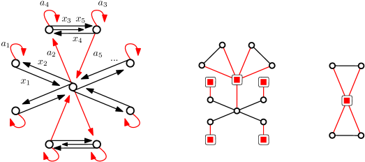
Figure 6. Left: a labeled graph $T^{\pi}$ quotient of a cycle of length 28. Middle and right: the graph $\overline{\mathcal{GDC}}$ of deterministic components with edge multiplicity forgotten and its pruning $\mathcal{P}run({\mathcal{GDC}})$. Note the subgraph $T^{\pi}_{A}$ (in red) has a connected component whose graph of t.e.c.c. have 4 leaves.

If $\overline{\mathcal{GDC}_{i}}$ is not a tree and its pruning $\mathcal{P}run({\mathcal{GDC}_{i}})$ is a non trivial graph. Recall the notation $\mathfrak{f}(C)$ from Definition 14 for the number of leaves in forest of two-edge connected components of $C$.

Lemma 30.

Let $C$ be a deterministic component of $T^{\pi}$.

1. If $C$ is suppressed by the pruning process, it has no cutting edge.

2. If $C$ is a vertex of $\mathcal{P}run({\mathcal{GDC}_{i}})$, then $\mathfrak{f}(C)\leq\text{deg}(C)$, where $\mathrm{deg}$ means the degree of the vertex in the graph $\mathcal{P}run({\mathcal{GDC}_{i}})$.

Taking for granted Lemma 30 momentarily, we conclude the proof of Lemma 24: assume that $\overline{\mathcal{GDC}_{i}}$ is not a tree and let us prove that necessarily $q_{2,i}+q_{2,i}^{\prime}\leq 0$. Note that when pruning a graph we suppress one edge for each leaf, so we have

$$q_{2,i}=\big{(}|\mathcal{V}_{i}|-|\bar{\mathcal{E}}_{i}|\big{)}=\big{(}|\widetilde{\mathcal{V}}_{i}|-|\widetilde{\mathcal{E}}_{i}|\big{)}.$$

Moreover, as for $\mathcal{GDC}_{i}$, the graph $\mathcal{P}run({\mathcal{GDC}}_{i})$ has vertices of two kinds, according to Definition 18. We denote by $\widetilde{\mathcal{V}}_{X,i}$ the set of vertices coming from the vertex set of $T^{\pi}$, and by $\widetilde{\mathcal{V}}_{A,i}$ the set of vertices coming from the connected components of $T^{\pi}_{A}$. Recall the classical formula in graph theory $|\widetilde{\mathcal{E}}_{i}|=\sum_{v\in\widetilde{\mathcal{V}}_{i}}\frac{\mathrm{deg}\,v}{2}$, where $\mathrm{deg}\,v$ is the number of neighbours of $v$ in $\mathcal{P}run({\mathcal{GDC}_{i}})$. We hence get

$$q_{2,i}+q_{2,i}^{\prime}=\big{(}|\widetilde{\mathcal{V}}_{i}|-|\widetilde{\mathcal{E}}_{i}|\big{)}+\Big{(}\frac{\mathfrak{f}(T^{\pi}_{A})}{2}-|C_{A}|\Big{)}$$

$$= \sum_{v\in\widetilde{\mathcal{V}}_{X,i}}\Big{(}1-\frac{\mathrm{deg}\,v}{2}\Big{)}+\sum_{C\in\widetilde{\mathcal{V}}_{A,i}}\Big{(}1-\frac{\mathrm{deg}\,C}{2}\Big{)}+\sum_{C\in C_{A,i}}\Big{(}\frac{\mathfrak{f}(C)}{2}-1\Big{)}.$$

In the above formula, $C_{A,i}$ denotes the set of connected components of $T^{\pi}_{A}$ which belongs to $\mathcal{GDC}_{i}$. The first part of Lemma 30 implies that the deterministic components $C$ that are erased by the pruning process satisfies $\mathfrak{f}(C)=2$. Hence in the right hand side of the above formula the last sum can be restricted to the sum over $C\in\widetilde{\mathcal{V}}_{A,i}$

$$q_{2,i}+q_{2,i}^{\prime}=\sum_{v\in\widetilde{\mathcal{V}}_{X,i}}\Big{(}1-\frac{\mathrm{deg}\,v}{2}\Big{)}+\sum_{C\in\widetilde{\mathcal{V}}_{A,i}}\Big{(}\frac{\mathfrak{f}(C)}{2}-\frac{\mathrm{deg}\,C}{2}\Big{)}.$$

Since $\mathcal{P}run({\mathcal{GDC}}_{i})$ has no leaves we have $\mathrm{deg}\,v\geq 2$ for any $v\in\widetilde{\mathcal{V}}_{X,i}$, and the second part of Lemma 30 states that $\mathfrak{f}(C)\leq\mathrm{deg}\,C$. This proves that $q_{2,i}+q_{2,i}^{\prime}\leq 0$ and finishes the proof of Lemma 24 - provided Lemma 30 holds true. $\square$

We now turn to the proof of Lemma 30, using the following notions.

Definition 31.

Let $S=(V,E)$ be a connected graph. We say that $\omega\in V$ is a cutting vertex of $S$ if there is a partition $V=V^{\prime}\sqcup\{\omega\}\sqcup V^{\prime\prime}$, $V^{\prime},V^{\prime\prime}\neq\emptyset$, such that there are no edge between a vertex of $V^{\prime}$ and a vertex of $V^{\prime\prime}$. Denoting by $S^{\prime}$ the subgraph of $S$ obtained by removing the vertices of $V^{\prime\prime}$ and the edges attached to it, we say that $S^{\prime}$ is a factor of $S$ with base $\omega$.

Lemma 32.

If $S$ is Eulerian, each factor of $S$ is Eulerian.

Proof.

Let $S^{\prime}=(V^{\prime},E^{\prime})$ be a factor of $S$ with base $\omega$. By Euler-Hierholzer theorem, all vertices $v\neq\omega$ have even degree in $S$. Since $S^{\prime}$ is factor, they have even degree in $S^{\prime}$. Moreover, the formula $|E^{\prime}|=\sum_{v\in V^{\prime}}\frac{\mathrm{deg}\,v}{2}$ implies $\mathrm{deg}\,\omega=2|E^{\prime}|-\sum_{v\neq\omega}\mathrm{deg}\,v$ so $\mathrm{deg}\,\omega$ is even. Hence $S^{\prime}$ is Eulerian. ∎

Proof of Lemma 30.

Let $S$ denote the $i$-th component of $T^{\pi}$. To prove the first part of the lemma we decompose the pruning process of $\overline{\mathcal{GDC}_{i}}$, and construct a sequence of factors $S^{(1)},S^{(2)},\dots,S^{(m)}=S^{(max)}$ of $S$ as follows. Note first that each suppression of a leaf in the pruning process either removes

• ($A$-step) a deterministic component $C$ and an associated edge $(v,C)$, for some $v$ of $T^{\pi}_{X}$;

• ($X$-step) or a vertex $v$ of $T^{\pi}_{X}$ and the edge adjacent to it.

Assume the first leaf suppression is an $A$-step that removes the vertex $C$ and the edge $(v,C)$ in $\overline{\mathcal{GDC}_{i}}$. We then set $S^{(1)}$ the graph obtained from $S$ by removing all edges of $C$ and the vertices that remain isolated after this removal. Necessarily $v$ is a cutting vertex so $C$ and $S^{(1)}$ are factors of $S$. Lemma 32 implies that $C$ is Eulerian, and so has no cutting edge. If the first leaf suppression is an $X$-step that removes the vertex $v$, we set $S^{(1)}$ the graph obtained from $S$ by removing the vertex $v$ and its adjacent edge. It is also a factor of $S^{(0)}$.

We pursue this construction with $S^{(1)}$ instead of $S$, getting iteratively a sequence of factors $S^{(1)},S^{(2)},\dots S^{(m)}=S^{(max)}$. This shows inductively that the deterministic components removed by the pruning process have no cutting edge. We have proved the first part of Lemma 30.

We now prove the second part of Lemma 30. Note for the sequel that by Lemma 32 the last factor $S^{(max)}$ of $S$ is an Eulerian graph. We now assume that $C$ is a deterministic component that is a vertex of $\mathcal{P}run({\mathcal{GDC}_{i}})$, i.e. it has not been removed by the pruning process. It is a deterministic component of $S^{(max)}$, but it is not a factor. We show that its degree in $\mathcal{P}run({\mathcal{GDC}_{i}})$ is not smaller than $\mathfrak{f}(C)$. Since $\mathcal{P}run({\mathcal{GDC}_{i}})$ has no leaves, then $\mathrm{deg}\,C\geq 2$, hence the property is obvious if $\mathfrak{f}(C)=2$. Assume from now that $\mathfrak{f}(C)\geq 3$ and, for a contradiction, that $\mathrm{deg}\,C<\mathfrak{f}(C)$.

Let $C^{\prime}$ be a two-edge connected component of $C$, that is a leaf in the tree $\mathcal{T}ec(C)$ of two-edge connected components of $C$. Since $C^{\prime}$ is a leaf of $\mathcal{T}ec(C)$, it is a factor of $C$ or a group of self-loops based on a vertex $\omega$ adjacent to a cutting edge. Since $\mathrm{deg}\,C<\mathfrak{f}(C)$ we can find such a $C^{\prime}$ that has no vertex adjacent to an edge labeled by a Wigner matrix in $S^{(max)}$. Thus no vertex of $C^{\prime}\setminus\{\omega\}$ is adjacent to an edge of $S^{(max)}\setminus C^{\prime}.$ This means that either $C^{\prime}$ is a factor of $S^{(max)}$ or $C^{\prime}$ is a group of self-loops. Since $S^{(max)}$ is Eulerian, then $C^{\prime}$ is Eulerian: all vertices of $C^{\prime}$ have even degree in $C^{\prime}$. But in $S^{(max)}$ the vertex $\omega$ is also adjacent to a cutting edge, so its degree in $S^{(max)}$ is its degree in $C^{\prime}$ increased by one: $S^{(max)}$ has a vertex of odd degree, which is in contradiction with Euler-Hierholzer theorem. This concludes the proof of Lemma 30 ∎

Proving Lemma 30 validates the proof of Lemma 24, and then the proof of the main result of this section, namely Proposition 22.

4. Characterization of the limit

4.1. Asymptotic formula

In this section, we only consider the asymptotics of $\tau^{(2)}$ and do not consider again the statistics $\tau^{(1)}$ of first order. We denote simply $\omega_{X}$ for the weight $\omega_{X}^{(2)}$ associated to Wigner matrices of Definition 11.

Let $\bm{Z}$ be a collection of Gaussian random variables, and assume that $\bm{Z}$ is stable by complex conjugate, that is $Z\in\bm{Z}$ implies $\overline{Z}\in\bm{Z}$. We recall that $\bm{Z}$ is Gaussian whenever it satisfies Wick formula: for any $n\geq 2$ and any $Z_{1},\dots,Z_{n}\in\bm{Z}$:

(32) $$\mathrm{E}[Z_{1}\cdots Z_{n}]=\sum_{\sigma\in\mathcal{P}_{2}(n)}\prod_{\{i,j\}\in\sigma}\mathrm{E}[Z_{i}Z_{j}],$$

where $\mathcal{P}_{2}(n)$ denotes the set of pairings of $[n]$, i.e. partitions whose blocks all have size two. In above formula, the product is over all blocks $\{i,j\}$ of the pairing $\sigma$.

We prove that $\tau^{(2)}$ is asymptotically Gaussian and give an asymptotic formula for the second order distribution in the following Proposition.

Proposition 33.

For any pair $\{i,j\}$ of indices, we denote by $\mathcal{P}(i,j)$ the set of partitions $\pi$ of the vertex set of $T_{i}\sqcup T_{j}$ with the following properties:

1. Either $(T_{i}\sqcup T_{j})^{\pi}$ is of double unicyclic type, and both graphs $\overline{\mathcal{GDC}}(T^{\pi}_{i})$ and $\overline{\mathcal{GDC}}(T^{\pi}_{j})$ are unicyclic. Hence the two latter cycles correspond to the same number $K\geq 1$ of edges associated to Wigner matrices (possibly intertwined with edges associated to deterministic matrices) and the cycle of $\overline{\mathcal{GDC}}\big{(}(T_{i}\sqcup T_{j})^{\pi}\big{)}$ is then obtained by twining pair-wise these $K$ edges of these cycles.

2. Either $(T_{i}\sqcup T_{j})^{\pi}$ is of 2-4 tree type, and both graphs $T^{\pi}_{i}$ and $T^{\pi}_{j}$ are of double tree type. A pair $\bar{e}_{i}$ of twin edges of $T^{\pi}_{X,i}$ and a pair $\bar{e}_{j}$ of twin edges of $T^{\pi}_{X,j}$ are then twined to form a group of edges of multiplicity 4 in $(T_{i}\sqcup T_{j})^{\pi}$.

3. In each case, twin edges associated to Wigner matrices in $(T_{i}\sqcup T_{j})^{\pi}$ are associated to a same Wigner matrix.

Then we have

$$\tau^{(2)}=\sum_{\sigma\in\mathcal{P}_{2}(n)}\prod_{\{i,j\}\in\sigma}\tau_{con}^{(2)}(i,j)+o(1),$$

with

(33) $$\tau_{con}^{(2)}(i,j)=\sum_{\begin{subarray}{c}\pi\in\mathcal{P}(i,j)\end{subarray}}\omega_{X}(\pi)\omega_{A}(\pi).$$

The contributions $\omega_{X}=\omega_{X}^{(2)}$ and $\omega_{A}(\pi)$ are computed by taking $T=T_{i}\sqcup T_{j}$ in Definitions 11 and 13.

The notation $\tau_{con}^{(2)}$ serves to emphasize that the quotient graph is connected. The rest of the subsection is devoted to the proof of Proposition 33. Let $\pi$ be a valid partition. We denote by $\sigma=\sigma(\pi)$ the partition of $[n]$ such that $B=\{\ell_{1},\dots,\ell_{p}\}$ is a block of $\sigma$ whenever there is a connected component of $T^{\pi}$ formed by these graphs $T^{\pi}_{\ell_{1}},\dots,T^{\pi}_{\ell_{p}}$. By the $X$-connectedness criterion of Lemma 26, if $\omega_{X}(\pi)\neq 0$ then $\sigma$ has no singletons.

By independence of the Wigner matrices and of the entries, we have $\omega_{X}(\pi)=\prod_{B\in\sigma}\omega_{X}(\pi_{B})$, where $\omega_{X}(\pi_{B})$ is defined by taking $T=\sqcup_{j\in B}T_{j}$ in Definition 11. The similar property for $\omega_{A}(\pi)$ up to a negligible error term follows from the next lemma.

Lemma 34.

Let $\pi\in\mathcal{P}(V)$ be a partition such that the components of $T^{\pi}_{A}$ are two-edge connected. Recalling that $C_{A}=C_{A}(\pi)$ is the set of connected components of $T^{\pi}_{A}$, we then have

$$\frac{1}{N^{|C_{A}|}}\mathrm{Tr}^{0}[T^{\pi}_{A}]=\prod_{C\in C_{A}}\frac{1}{N}\mathrm{Tr}^{0}[C]+o(1).$$

Proof.

We write $\pi\leq\pi^{\prime}$ to mean that the blocks of $\pi$ are included in the blocks of $\pi^{\prime}$, and so $T^{\pi^{\prime}}$ is a quotient of $T^{\pi}$. With notations as in the lemma, we have

$$\frac{1}{N^{|C_{A}|}}\mathrm{Tr}^{0}[T^{\pi}_{A}]=\frac{1}{N^{|C_{A}|}}\sum_{\begin{subarray}{c}\pi\leq\pi^{\prime}\in\mathcal{P}(V)\\ \mathrm{injective}\end{subarray}}r(T_{A},\pi^{\prime})$$

and

$$\prod_{C\in C_{A}}\frac{1}{N}\mathrm{Tr}^{0}[C]=\frac{1}{N^{|C_{A}|}}\prod_{C\in C_{A}}\sum_{\begin{subarray}{c}\pi^{\prime}\in\mathcal{P}(V_{C})\\ \mathrm{injective}\end{subarray}}r(C_{A},\pi^{\prime})$$

Hence

$$\frac{1}{N^{|C_{A}|}}\mathrm{Tr}^{0}[T^{\pi}_{A}]-\prod_{C\in C_{A}}\frac{1}{N}\mathrm{Tr}^{0}[C]=-\frac{1}{N^{|C_{A}|}}\sum_{\pi^{\prime}}r(T_{A},\pi^{\prime})$$

where the sum is over all $\pi\leq\pi^{\prime}\in\mathcal{P}(V)$, whose restriction on each connected component of $T^{\pi}_{A}$ is injective, but which is not injective. Hence such a choice reduces the number of connected components. Since the graphs are two-edge connected, with the bound of Mingo and Speicher from [17] we deduce that $\sum_{\pi^{\prime}}r(T_{A},\pi^{\prime})=O(N^{|C_{A}|-1})$. ∎

From (29), by additivity of the topological parameters and by asymptotic multiplicativity of the $\omega$-functions we can then deduce an asymptotic factorization with respect to connected components

(34) $$\tau^{(2)}=\sum_{\sigma\in\mathcal{P}(n)}\prod_{B\in\sigma}\sum_{\begin{subarray}{c}\pi\in\mathcal{P}(\sqcup_{j\in B}V_{j})\\ \mathrm{valid,\ connected}\end{subarray}}\omega_{X}(\pi)\omega_{A}(\pi)+o(1),$$

where the $\omega$-functions are defined by taking $T=\sqcup_{j\in B}T_{j}$ in Definitions 11 and 13, and we can assume $|B|\geq 2$ for all blocks $B$ of $\sigma$.

Lemma 35.

Let $\pi$ be a valid partition such that $\omega_{X}(\pi)\neq 0$ and assume that the $i$-th connected component of $T^{\pi}$ of double cycle type. Then, there are two different cycles $T_{j},T_{j^{\prime}}$, $j\neq j^{\prime}\in[n]$, such that each a group of twin edges of $T^{\pi}_{X}$ in the cycle of $\overline{\mathcal{GDC}_{i}}$ consists of an edge from $T_{j}$ and an edge from $T_{j^{\prime}}$.

Proof.

Denote by $E_{0}$ the set of groups of twin edges labeled by Wigner matrices in the cycle of $\overline{\mathcal{GDC}_{i}}$. Assume that a cycle $T_{j}$ has exactly one edge labeled by a Wigner matrix in a group $\bar{e}\in E_{0}$ of adjacent edges. For a contradiction, assume moreover that there is another group edges $\bar{e}^{\prime}\in E_{0}$ in the cycle that comes from others cycle $T_{j^{\prime}},T_{j^{\prime\prime}}$, $j^{\prime}\neq j\neq j^{\prime\prime}$. We denote by $T^{\pi}\setminus{\bar{e}^{\prime}}$ the graph obtained from $T^{\pi}$ by removing the two edges of $\bar{e}^{\prime}$. Since the removal does disconnect the graph nor change the parity of vertices, $T^{\pi}\setminus{\bar{e}^{\prime}}$ is an Eulerian graph. The removal of the edges of $\bar{e}$ disconnects $T^{\pi}\setminus{\bar{e}^{\prime}}$. The fact that a single edge of $T_{j}$ belongs to $\bar{e}$ is hence in contradiction with the parity argument of Lemma 20. This implies that all $T_{j}$ has one edge in element of $E_{0}$, and so another graph $T_{j^{\prime}}$ has the same property.

To finish the proof of lemma, we now assume that each group of edges in $E_{0}$ comes from a single cycle. Since all group of edges labeled by Wigner matrices out of the cycle are of multiplicty 2, Lemma 20 implies that each group of twin edges of the $i$-th component of $T^{\pi}$ labeled by Wigner matrices come from a cycle. The $X$-connectedness criterion (Lemma 26) hence implies $\omega_{X}(\pi)=0$. ∎

We can now finish the proof of Proposition 33. Assume for $\pi$ valid that a component $S$ of $T^{\pi}$ is made of at least 3 graphs among $T^{\pi}_{1},\dots,T^{\pi}_{n}$ and let us prove that $\omega_{X}(\pi)=0$.

• Assume $S$ is of 2-4 tree type. By the parity argument, only the edge labeled by Wigner matrices of multiplicity 4 can come from two graphs, so at least one graph is $X$-disconnected from all other graphs and Lemma 26 implies $\omega_{X}(\pi)=0$.

• Assume $S$ is of double unicyclic type. By Lemma 35, only the edge labeled by Wigner matrices that belongs to the groups in the cycle of $\overline{\mathcal{GDC}}(S)$ can come from two graphs, and the same conclusion holds.

Hence in Formula (34) we can restrict the sum to pairings $\sigma\in\mathcal{P}_{2}(n)$. That the only pairings $\sigma$ for which $\omega_{X}(\pi)\neq 0$ are those such that the blocks $\{i,j\}$ of $\sigma$ are in $\mathcal{P}(i,j)$ is a consequence of same arguments of $X$-connectedness as before. Finally, by independence of the matrices and the centeredness in the definition of $\omega_{X}$, we have $\omega_{X}(\pi)=0$ when there exist twin edges associated to different Wigner matrices. This finishes the proof of Proposition 33.

4.2. Computation of the covariance: even moments and vanishing pseudo-variance

By Proposition 33, in the sequel we can assume $n=2$, so $T=T_{1}\sqcup T_{2}$ is the union of 2 simple cycles. We shall compute the limit of $\tau^{(2)}_{con}(1,2)$ defined in Equation (33) and prove the covariance formulas of Theorems 5 and 6. We use the shorthand $\tau^{(2)}_{con}:=\tau^{(2)}_{con}(1,2)$.

By Proposition 33 and Lemma 34, we have

(35) $$\tau_{con}^{(2)}=\sum_{\pi\in\mathcal{P}(1,2)}\omega_{X}(\pi)\prod_{C\in C_{A}}\frac{1}{N}\mathrm{Tr}^{0}[C]+o(1),$$

where $\pi\in\mathcal{P}(1,2)$ means that $T^{\pi}$ is of double unicyclic or 2-4 tree type graph as in Definition 21, and $C_{A}=C_{A}(\pi)$ denotes the set of connected components of $T^{\pi}_{A}$. We denote by $2m$ and $2n$ the lengths of the cycles $T_{1}$ and $T_{2}$ respectively (they are even since the letters $X_{i}$ and $A_{i}$ alternated in Definition 22 of the matrices $M_{j}$). By a simple parity argument for the number of double edges coming from $T_{1}$ and $T_{2}$, if $m$ and $n$ do not have the same parity, there is no $\pi\in\mathcal{P}(V^{\pi})$ such that $T^{\pi}$ is of double unicyclic or 2-4 tree type, and so $\tau_{con}^{(2)}\underset{N\rightarrow\infty}{\longrightarrow}0$.

In this section, we assume that $m$ and $n$ are even. Assume that $T^{\pi}$ is of double unicyclic type graph. We claim that the double cycle of $\mathcal{GDC}(T^{\pi})$ has an even number $2\ell$ of double edges labeled by Wigner matrices, for $\ell\geq 1$. Indeed, each $T_{i}$ has an even total number of edges. It has also an even number of edges out of the cycle and there is exactly one edge of each $T_{i}$ for each double edge of the cycle. We use in the sequel the idea that a 2-4 tree type graph is a degenerated version of a double unicyclic type graph with $2\ell=2$. This consideration is important latter since the expression (35) depends on the injective traces $\mathrm{Tr}^{0}[C]$ whereas we want an expression in terms of the parameters of the deterministic matrices, i.e. normalized traces of entry-wise products.

4.2.1. Computation of weights $\omega_{X}$

Definition 36.

1. We say that two twin edges $e_{1}$ and $e_{2}$ are opposite if the source of $e_{1}$ is the target of $e_{2}$ and reciprocally, and that they are parallel if they have same source and same target.

2. Let $\pi\in\mathcal{P}(1,2)$ such that $T^{\pi}$ is of double unicyclic type. We say that $T^{\pi}$ is of opposite type if all twin edges of $T^{\pi}_{X}$ are opposite, and of parallel type otherwise.

For a parallel type graph, twin edges labeled by a Wigner matrix on the double cycle are all parallel, twin edges outside the double cycle are always opposite.

We compute easily the value of $\omega_{X}(\pi)$ from its definition in Eq. (23).

• Let $\mathcal{DU}^{opp}$ denote the set of partitions $\pi\in\mathcal{P}(1,2)$ such that $T^{\pi}$ is of opposite double unicyclic type. Since all entries of Wigner matrices have normalized variance, for $\pi\in\mathcal{DU}^{opp}$ we have

  (36) $$\omega_{X}(\pi)=1.$$

• Let $\mathcal{FT}$ denote the set of $\pi\in\mathcal{P}(1,2)$ such that $T^{\pi}$ is of 2-4 tree type. Then $\pi\in\mathcal{FT}$ implies

  (37) $$\omega_{X}(\pi)=\mathrm{E}[|x^{(\pi)}_{12}|^{4}]-1,$$

  where $X^{(\pi)}=\big{(}\frac{x^{(\pi)}_{ij}}{\sqrt{N}}\big{)}_{ij}$ stands for the Wigner matrix associated to the edge of multiplicity 4 in $T^{\pi}_{X}$.

• Let $\mathcal{DU}^{par}$ the set of partitions $\pi\in\mathcal{P}(1,2)$ such that $T^{\pi}$ is of parallel double cyclic type. For all $\pi\in\mathcal{DU}^{par}$ we have

  (38) $$\omega_{X}(\pi)=\theta(\pi):=\prod_{k=1}^{K}\mathrm{E}[{x^{(i_{k})}_{12}}^{2}],$$

  where $X^{(i_{k})}=\big{(}\frac{x^{(i_{k})}_{ij}}{\sqrt{N}}\big{)}_{ij}$, $k=1,\dots,K$, stands for the Wigner matrices associated to the double cycle.

From now and until the rest of Section 4.2, we also assume that the Wigner matrices have null pseudo-variance. Hence $\theta(\pi)$ in (38) vanishes and we get from (35)

$$\tau^{(2)}_{con} = \sum_{\pi\in\mathcal{DU}^{opp}}\bigg{(}\prod_{C\in C_{A}(\pi)}\frac{1}{N}\mathrm{Tr}^{0}[C]\bigg{)}$$

$$+\sum_{\pi\in\mathcal{FT}}\bigg{(}\big{(}\mathrm{E}[|x^{(\pi)}_{12}|^{4}]-1\big{)}\prod_{C\in C_{A}(\pi)}\frac{1}{N}\mathrm{Tr}^{0}[C]\bigg{)}+o(1).$$

The aim is now to see how appear the parameters of the deterministic components. For that given a partition $\pi$ we associate a graph $G^{\pi}_{X}$ whose edges are labeled by the Wigner matrices and a graph $G^{\pi}_{A}$ labeled by the deterministic matrices. Recall that $T^{\pi}_{X}$ (resp. $T^{\pi}_{A}$) is the subgraph of $T^{\pi}$ whose edges are labeled by the Wigner (resp. deterministic) matrices.

Definition 37.

Let $\pi\in\mathcal{P}(1,2)$. We denote $G^{\pi}_{X}$ the graph labeled by Wigner matrices obtained from $T^{\pi}$ by contracting the edges labeled by deterministic matrices to vertex: we identify the source and the target for each of those edges and we remove them. We denote $G^{\pi}_{A}$ the graph labeled by deterministic matrices that is the smallest quotient $T^{\pi_{0}}_{A}$ such that $G^{\pi}_{X}=G^{\pi_{0}}_{X}$.

Let $\mathcal{G}=\mathcal{G}(n,m)$ denote the set of all possible graphs $G^{\pi}_{X}$ for $\pi\in\mathcal{P}(i,j)$. We also set

$$\mathcal{G}^{opp} = \{G^{\pi}_{X}\in\mathcal{G}\,|\,\pi\in\mathcal{DU}^{opp}\}.$$

4.2.2. Opposite type, first case

For any $\ell\geq 1$, we denote by $\mathcal{DU}^{opp}_{\ell}$ (resp. $\mathcal{G}^{opp}_{\ell})$ the set of partitions $\pi\in\mathcal{DU}^{opp}$ (of graphs $G^{\pi}_{X}$) such that there are $\ell$ double edges labeled by Wigner matrices in the double cycle.

Figure 7. Left: a labeled graph $T^{\pi}$ such that $\pi\in\mathcal{DU}^{opp}_{4}$. Right: the graph $G^{\pi}_{X}$.

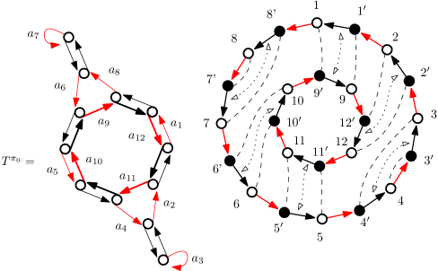
Figure 8. Left: The graph $T^{\pi_{0}}$ for the minimal partition $\pi_{0}$ such that $G_{X}(\pi_{0})=G^{\pi}_{X}$ where $\pi$ is as in Figure 7. Note that $G^{\pi}_{A}$ consists of the union of the components of $T^{\pi_{0}}$ labeled by deterministic matrices. Right: the annulus $\mathcal{A}nn^{opp}$, with dashed lines to represent to identifications of vertices made by $\pi_{0}$, and dotted lines with arrows to represent the partition $\sigma_{G^{\pi}_{X}}$.

Let $G\in\mathcal{G}^{opp}_{2\ell}$ for $\ell\geq 2$. All partitions $\pi$ such that $G^{\pi}_{X}=G$ have same graph $K(G):=G^{\pi}_{A}$ that we call the complement of $G$. The connected components of this graph $K(G)$ are simple oriented cycles $C_{1},\dots,C_{k}$. Each partition $\pi\in\mathcal{P}(1,2)$ such that $G^{\pi}_{A}=K(G)$ corresponds to a $k$-tuple $(\pi_{1},\dots,\pi_{k})$ where $\pi_{i}$ is a partition of $C_{i}$. The relation between trace and injective trace of graphs implies (with $V_{C_{i}}$ the vertex set of the $i$-th cycle $C_{i}$ of $K(G)$)

$$\sum_{\begin{subarray}{c}\pi\in\mathcal{DU}^{opp}_{2\ell}\\ \mathrm{s.t.\ }G^{\pi}_{X}=G\end{subarray}}\prod_{C\in C_{A}(\pi)}\frac{1}{N}\mathrm{Tr}^{0}[C] = \prod_{i=1}^{k}\sum_{\pi_{i}\in\mathcal{P}(V_{C_{i}})}\frac{1}{N}\mathrm{Tr}^{0}[C_{i}^{\pi}]=\prod_{i=1}^{k}\frac{1}{N}\mathrm{Tr}[C_{i}].$$

We now associate to any graph $G\in\mathcal{G}^{opp}_{2\ell}$ a pairing $\sigma_{G}\in NC_{2}^{(2\ell)}(m,n)$, where we recall that $m$ and $n$ are the lengths of $T_{1}$ and $T_{2}$ respectively.

Definition 38.

We denote by $\mathcal{A}nn^{opp}$ the labeled graph $T$ embedded in $\mathbb{C}$ that consists of the annulus formed by the outer cycle $T_{1}$ in anticlockwise orientation, and the inner cycle $T_{2}$ in clockwise orientation. For any $G\in\mathcal{G}^{opp}$, we set $\sigma_{G}$ the pairing of the edge set of $\mathcal{A}nn^{opp}$ labeled by Wigner matrices such that two edges belong to a same block if and only if they are twined in $G$.

By contracting the $A$-edges of $\mathcal{A}nn^{opp}$, we see $\sigma_{G}$ as an annulus partition of $(m,n)$ elements represented by the edges labeled $X_{1},\dots,X_{m+n}$. Recall that $\sigma\in NC_{2}^{(2\ell)}(m,n)$ is non-mixing if twin edges are always labeled by a same Wigner matrix.

Lemma 39.

The pairing $\sigma_{G}$ is non crossing, and the function $G\mapsto\sigma_{G}$ defines a bijection from $\mathcal{G}^{opp}_{2\ell}$ to the set of non-mixing elements of $NC_{2}^{(2\ell)}(m,n)$.

Proof.

Let $G=G_{X}(\pi)\in\mathcal{G}^{opp}_{2\ell}$. If each edge labeled by a Wigner matrix in $T_{1}$ is twinned in $T^{\pi}$ with an edge of $T_{2}$ (so $\overline{\mathcal{GDC}}$ is a cycle), then $\sigma_{G}$ is a spoke diagram: necessarily $n=m$ and there is an index $j_{0}$ such that the $j$-th edge of $T_{1,X}$ is twinned in $T^{\pi}$ with the $j+j_{0}$-th edge of $T_{2,X}$, for any $j$ with notations modulo $n$. Hence $\sigma_{G}$ is a non crossing pairing.

Otherwise, they are edges labeled by Wigner matrices in $T_{1}$ or in $T_{2}$ that are twinned together, and so $T^{\pi}$ has double tree type factor. Recall that an annular partition of is non-crossing if and only if either it is a spoke diagram, or it has a block of the form $\{i,i+1,\dots,i+j\}$ in $[n]$ or $[m]$, and the removal of this blocks yields another non-crossing partition [19], Remark 9.2. The pruning process shows that this nesting property is satisfied by $\sigma_{G}$.

Hence every $G\in G^{opp}_{2\ell}$ yields an element of $NC_{2}^{(2\ell)}(m,n)$. It is non mixing by the third condition in the definition of $\mathcal{P}(i,j)$ (Proposition 33). Reciprocally, if $\sigma$ is a pairing in $NC_{2}^{(2\ell)}(m,n)$, it gives a way to identify pairwise the edges of $\mathcal{A}nn^{opp}$, and if $\sigma=\sigma_{G}$ then contracting the $A$-edges yields correctly the graph $G$. ∎

Let $G=G^{\pi}_{X}\in\mathcal{G}^{opp}_{2\ell}$ and $K(G)=G^{\pi}_{A}$ its complement introduced above. We consider the partition of the edge set of $\mathcal{A}nn^{opp}$ labeled by deterministic matrices such that two edges belong to a same block if and only if they belong to a same cycle of $G^{\pi}_{A}$. Then this partition is actually the Kreweras complement $K(\sigma_{G})$ of $\sigma_{G}$. Moreover, denoting by $C_{1},\dots,C_{k}$ the cycles of $K(G)=G^{\pi}_{A}$, then

$$\prod_{i=1}^{k}\frac{1}{N}\mathrm{Tr}[C_{i}]\underset{N\rightarrow\infty}{\longrightarrow}\varphi_{K(\sigma_{G})}(a_{1},\dots,a_{m+n}),$$

where $\varphi_{K(\sigma)}$ is as in the statement of Theorem 5. We hence have proved for $\ell\geq 2$

$$\sum_{G\in\mathcal{G}^{opp}_{2\ell}}\sum_{\begin{subarray}{c}\pi\in\mathcal{DU}^{opp}_{2\ell}\\ \mathrm{s.t.\ }G^{\pi}_{X}=G\end{subarray}}\prod_{C\in C_{A}}\frac{1}{N}\mathrm{Tr}^{0}[C]\underset{N\rightarrow\infty}{\longrightarrow}\sum_{\begin{subarray}{c}\sigma\in NC_{2}^{(2\ell)}(m,n)\\ \mathrm{non-mixing}\end{subarray}}\varphi_{K(\sigma)}(a_{1},\dots,a_{m+n}).$$

4.2.3. 4-2 type

We set $\mathcal{G}^{FT}$ the set of graphs $G$ of the form $G=G^{\pi}_{X}$ where $\pi\in\mathcal{FT}$, i.e. $T^{\pi}$ is of 4-2 tree type, and fix $G\in\mathcal{G}^{FT}$.

Figure 9. Left: a labeled graph $T^{\pi}$ such that $\pi\in\mathcal{T}^{42}$. Right: the graph $G^{\pi}_{X}$.

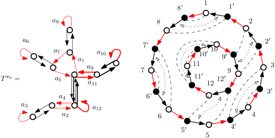
Figure 10. Left: The graph $T^{\pi_{0}}$ for the minimal partition $\pi_{0}$ such that $G_{X}(\pi_{0})=G^{\pi}_{X}$ where $\pi$ is as in Figure 9. Edges of $T_{1}$ (resp. $T_{2}$) are the thin (resp. thick) ones. Right: the annulus $\mathcal{A}nn^{opp}$, with dashed lines to represent to identifications of vertices made by $\pi_{0}$, and dotted lines with arrows to represent the pairing $\sigma_{G^{\pi}_{X}}$.

For any $\pi$ such that $G^{\pi}_{X}=G$, the graph $K(G)=G^{\pi}_{A}$ depends only on $G$. Since $G$ is a fat tree (forgetting the multiplicity of edges yields a tree), it has one edge of multiplicity 4 and the other edges are of multiplicity two, the graph $K(G)$ consists in a union of cycles $C_{1},\dots,C_{k}$ and of two subgraphs $C_{k+1}$ and $C_{k+2}$ (adjacent to the edge of multiplicity 4 in the minimal graph $T^{\pi_{0}}$). Each of these subgraphs $C_{k+1}$ and $C_{k+2}$ consists of two simple directed cycles identified by one vertex. The partitions $\pi^{\prime}$ such that $G_{A}^{\pi^{\prime}}=G^{\pi}_{A}$ are in correspondence with the $k$-tuples $(\pi_{1},\dots,\pi_{k+2})$ where $\pi_{i}$ is a partition of the vertex set of $C_{i}$. Hence we get

$$\sum_{\begin{subarray}{c}\pi\in\mathcal{FT}\\ \mathrm{s.t.\ }G^{\pi}_{X}=G\end{subarray}}\prod_{C\in C_{A}}\frac{1}{N}\mathrm{Tr}^{0}[C]=\prod_{i=1}^{k+2}\frac{1}{N}\mathrm{Tr}[C_{i}].$$

We associate to $G\in\mathcal{G}^{FT}$ a partition $\sigma_{G}\in NC_{2}^{(2)}(m,n)$.

Definition 40.

With $\mathcal{A}nn^{opp}$ as in Definition 38, for any $G\in\mathcal{G}^{FT}$, we set $\sigma_{G}$ the pair pairing of the edge set of $\mathcal{A}nn^{opp}$ labeled by Wigner matrices such that two edges $e,e^{\prime}$ belong to a same block if and only if

• they are twins in $G$,

• and moreover, if $e$ and $e^{\prime}$ belong to the group of edge of multiplicity 4, then $e$ and $e^{\prime}$ belong to the different cycles $T_{1}$ and $T_{2}$ and have opposite orientation.

The same arguments as before show that $\sigma_{G}$ for $G\in\mathcal{G}^{FT}$ is a non-mixing non-crossing annulus pairing with two through strings, and the map $G\mapsto\sigma_{G}$ is a bijection. The two ways to connect the through strings illustrated in Figure 2 represent the two ways to form a 4-2 tree by identifying a double edge from two double trees. Denoting as before by $C_{1},\dots,C_{k+2}$ the connected components of $K(G)$, we have

$$\prod_{i=1}^{k+2}\frac{1}{N}\mathrm{Tr}[C_{i}]\underset{N\rightarrow\infty}{\longrightarrow}\tilde{\varphi}_{K(\sigma_{G})}(a_{1},\dots,a_{m+n}),$$

where $\tilde{\varphi}_{K(\sigma)}$ is as in the statement of Theorem 5. The Hadamard products in the definition of $\tilde{\varphi}$ result from the components $C_{k+1}$ and $C_{k+2}$, point (2) from Proposition 33 (see also Figure 1). We hence get

$$\sum_{\pi\in\mathcal{FT}}\big{(}\mathrm{E}[|x^{(\pi)}_{12}|^{4}]-1\big{)}\prod_{C\in C_{A}}\frac{1}{N}\mathrm{Tr}^{0}[C]$$

$$\underset{N\rightarrow\infty}{\longrightarrow} \sum_{\begin{subarray}{c}\sigma NC_{2}^{(2)}(m,n)\\ \mathrm{non-mixing}\end{subarray}}\big{(}\mathrm{E}[|x^{(\sigma)}_{12}|^{4}]-1\big{)}\tilde{\varphi}_{K(\sigma_{G})}(a_{1},\dots,a_{m+n}),$$

where non-mixing means also that the 2 through strings are labeled by the same Wigner matrix $X^{(\sigma)}$. We emphasize that $\big{(}\mathrm{E}[|x^{(\sigma)}_{12}|^{4}]-1\big{)}$ is not the weight expected in Theorem 5.

4.2.4. Opposite type, second case

Let $G\in\mathcal{G}^{opp}_{2}$, namely $G=G^{\pi}_{X}$ for $T^{\pi}$ of double unicyclic type such that $\mathcal{GDC}(T^{\pi})$ has exactly 2 double edges labeled by a Wigner matrix on its double cycle. The graph $G$ is degenerated: as we contract the $A$-edges, the double cycle in $\mathcal{GDC}(T^{\pi})$ becomes an edge of multiplicity 4 in $G$. Hence $G$ is a 4-2 tree, namely a fat tree whose edges are all of multiplicity 2 but one is of multiplicity 4.

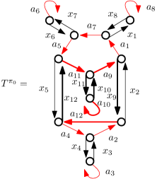
Figure 11. A labeled graph $T^{\pi}$ such that $\pi\in\mathcal{DU}^{opp}_{2}$. The graph $G^{\pi}_{X}$ is the same as the rightmost picture in Figure 9.

Nevertheless, as for $G\in\mathcal{G}^{opp}_{2\ell}$ for $\ell\geq 2$, it remains true that $G^{\pi}_{A}$ is a union of simple cycles $C_{1},\dots,C_{k}$. In this case yet there are partitions $\pi^{\prime}$ that factorize as disjoint partitions $\pi^{\prime}_{1},\dots,\pi^{\prime}_{k}$ of the different cycles $C_{i}$’s, but for which $G_{A}^{\pi^{\prime}}\neq G^{\pi}_{A}$: they are the partitions $\pi^{\prime}$ such that the two double edges of the double cycle are identified to form a group of edges of multiplicity 4. Hence they are the partitions $\pi^{\prime}\in\mathcal{FT}$ such that $G=G_{X}^{\pi^{\prime}}$. The graph $G_{A}^{\pi^{\prime}}$ is a union of $k-2$ cycles $\tilde{C}_{1},\dots,\tilde{C}_{k-2}$, where two graphs $\tilde{C}_{i}$ are obtained by identifying a vertex of cycle $C_{p}$ and a vertex of a cycle $C_{q}$.

We hence have

$$\sum_{\begin{subarray}{c}\pi\in\mathcal{DU}^{opp}_{2}\\ \mathrm{s.t.\ }G^{\pi}_{X}=G\end{subarray}}\prod_{C\in C_{A}(\pi)}\frac{1}{N}\mathrm{Tr}^{0}[C]$$

$$= \prod_{i=1}^{k}\sum_{\pi_{i}\in\mathcal{P}(V_{C_{i}})}\frac{1}{N}\mathrm{Tr}^{0}[C_{i}^{\pi}]-\sum_{\begin{subarray}{c}\pi\in\mathcal{FT}\\ \mathrm{s.t.\ }G^{\pi}_{X}=G\end{subarray}}\prod_{C\in C_{A}(\pi)}\frac{1}{N}\mathrm{Tr}^{0}[C]$$

$$= \prod_{i=1}^{k}\frac{1}{N}\mathrm{Tr}[C_{i}]-\prod_{i=1}^{k-2}\frac{1}{N}\mathrm{Tr}[\tilde{C}_{i}]$$

$$\underset{N\rightarrow\infty}{\longrightarrow} \varphi_{K(\sigma)}(a_{1},\dots,a_{m+n})-\tilde{\varphi}_{K(\sigma)}(a_{1},\dots,a_{m+n}).$$

As a conclusion, we have proved for $m$ and $n$ even and assuming null pseudo-variance for Wigner matrices, by (35)

$$\tau^{(2)}_{con} \underset{N\rightarrow\infty}{\longrightarrow} \sum_{\begin{subarray}{c}\sigma\in NC_{2}(m,n)\\ \text{non-mixing}\end{subarray}}\varphi(a_{1},\dots,a_{m+n})$$

$$\qquad+\sum_{\begin{subarray}{c}\sigma\in NC_{2}^{(2)}(m,n)\\ {non-mixing}\end{subarray}}\big{(}\mathrm{E}[|x^{(\sigma)}_{12}|^{4}]-2\big{)}\tilde{\varphi}_{K(\sigma)}(a_{1},\dots,a_{m+n}).$$

This is now indeed the expected formula (2) in Theorem 5.

4.3. Computation of the covariance: even moments, general pseudo-variance

We now have by (35), with $C_{A}=C_{A}(\pi)$,

$$\tau^{(2)}_{con} = \sum_{\pi\in\mathcal{DU}^{opp}}\prod_{C\in C_{A}}\frac{1}{N}\mathrm{Tr}^{0}[C]+\sum_{\pi\in\mathcal{FT}}\big{(}\mathrm{E}[|x^{(\pi)}_{12}|^{4}]-1\big{)}\prod_{C\in C_{A}}\frac{1}{N}\mathrm{Tr}^{0}[C]$$

$$+\sum_{\pi\in\mathcal{DU}^{par}}\theta(\pi)\prod_{C\in C_{A}}\frac{1}{N}\mathrm{Tr}^{0}[C]+o(1),$$

where $\theta(\pi)$ is defined in (38). As before, for any $\ell\geq 1$, we denote by $\mathcal{DU}^{par}_{2\ell}$ the set of partitions $\pi\in\mathcal{DU}^{par}$ with $2\ell$ double edges by Wigner matrices in the double cycle, and by $\mathcal{G}^{par}_{2\ell}$ the set of graphs $G\in\mathcal{G}$ of the form $G=G^{\pi}_{X}$ for some $\pi\in\mathcal{DU}^{par}_{2\ell}$.

Assume $G\in\mathcal{G}^{par}_{2\ell}$ for $\ell\geq 2$. As for elements of $\mathcal{G}^{opp}_{2\ell}$, all partitions $\pi$ such that $G^{\pi}_{X}=G$ have same graph $K(G):=G^{\pi}_{A}$, which consists of a union of simple oriented cycles $C_{1},\dots,C_{k}$, and such partitions $\pi$ are in correspondence with the $k$-tuples of partitions $(\pi_{1},\dots,\pi_{k})$ where $\pi_{i}$ is a partition of the vertex set of $C_{i}$. Moreover, for any $\pi$ such that $G^{\pi}_{X}=G$, $\theta(\pi)$ is completely determined by $G$ and shall be denoted $\theta(G)$. We hence get, as for the opposite case,

$$\sum_{\begin{subarray}{c}\pi\in\mathcal{DU}^{par}_{2\ell}\\ \mathrm{s.t.\ }G^{\pi}_{X}=G\end{subarray}}\theta(\pi)\prod_{C\in C_{A}}\frac{1}{N}\mathrm{Tr}^{0}[C] = \theta(G)\prod_{i=1}^{k}\sum_{\pi_{i}\in\mathcal{P}(V_{C_{i}})}\frac{1}{N}\mathrm{Tr}^{0}[C_{i}^{\pi}]$$

$$= \theta(G)\prod_{i=1}^{k}\frac{1}{N}\mathrm{Tr}[C_{i}].$$

Definition 41.

We denote by $\mathcal{A}nn^{par}$ the labeled graph consisting of the annulus formed by the outer cycle $T_{1}$ and the inner cycle $T_{2}$, both in in anticlockwise orientation. For any $G\in\mathcal{G}^{par}$, we set $\sigma_{G}$ the partition of the edge set of $\mathcal{A}nn^{par}$ labeled by Wigner matrices such that two edges belong to a same block if and only if they are twined in $G$.

As before, $\sigma_{G}$ is a non crossing pairing which completely determines $G$. We denote $\theta_{\sigma}=\theta(G)$ and get

$$\sum_{G\in\mathcal{G}^{par}_{2\ell}}\sum_{\begin{subarray}{c}\pi\in\mathcal{DU}^{par}_{2\ell}\\ \mathrm{s.t.\ }G^{\pi}_{X}=G\end{subarray}}\theta(G)\prod_{C\in C_{A}}\frac{1}{N}\mathrm{Tr}^{0}[C]$$

$$\underset{N\rightarrow\infty}{\longrightarrow} \sum_{\begin{subarray}{c}\sigma\in NC_{2}^{(2\ell)}(m,n)\\ \text{non-mixing}\end{subarray}}\theta_{\sigma}\varphi_{K(\sigma)}(a_{1},\dots,a_{m},a_{m+n}^{t},\dots,a_{m+1}^{t}).$$

Assume now that $G\in\mathcal{G}^{par}_{2}$. All $\pi$ such that $G^{\pi}_{X}=G$ have same graph $K(G):=G^{\pi}_{A}$ which consists in a union of cycles $C_{1},\dots,C_{k}$. There are partitions $\pi^{\prime}$ such that the two double edges of the double cycle are identified to form a group of edges of multiplicity 4, for which $G_{A}^{\pi^{\prime}}$ is a union of $k-2$ cycles $\tilde{C}_{1},\dots,\tilde{C}_{k-2}$, where two graphs $\tilde{C}_{i}$ are obtained by identifying a vertex of cycle $C_{p}$ and a vertex of a cycle $C_{q}$. As in the opposite case, we have

$$\sum_{\begin{subarray}{c}\pi\in\mathcal{DU}^{par}_{2}\\ \mathrm{s.t.\ }G^{\pi}_{X}=G\end{subarray}}\theta(\pi)\prod_{C\in C_{A}}\frac{1}{N}\mathrm{Tr}^{0}[C]$$

$$= \prod_{i=1}^{k}\sum_{\pi_{i}\in\mathcal{P}(V_{C_{i}})}\frac{1}{N}\mathrm{Tr}^{0}[C_{i}^{\pi}]$$

$$= \theta(G)\big{(}\prod_{i=1}^{k}\frac{1}{N}\mathrm{Tr}[C_{i}]-\prod_{i=1}^{k-2}\frac{1}{N}\mathrm{Tr}[\tilde{C}_{i}]\big{)}$$

$$\underset{N\rightarrow\infty}{\longrightarrow} \theta_{\sigma}\varphi_{K(\sigma)}(a_{1},\dots,a_{m},a_{m+n}^{t},\dots,a_{m+1}^{t})-\theta_{\sigma}\tilde{\varphi}_{K(\sigma)}(a_{1},\dots,a_{m+n}).$$

Finally, we obtain

$$\tau^{(2)}_{con} \underset{N\rightarrow\infty}{\longrightarrow} \sum_{\begin{subarray}{c}\sigma\in NC_{2}(m,n)\\ \text{non-mixing}\end{subarray}}\varphi_{{K(\sigma)}}(a_{1},\dots,a_{m+n})$$

$$\qquad+\sum_{\begin{subarray}{c}\sigma\in NC^{(2)}_{2}(m,n)\\ \text{non-mixing}\end{subarray}}\big{(}\mathrm{E}[|x^{(\sigma)}_{12}|^{4}]-2-\theta_{\sigma}\big{)}\tilde{\varphi}_{K(\sigma)}(a_{1},\dots,a_{m+n})$$

$$\qquad+\sum_{\begin{subarray}{c}\sigma\in NC_{2}(m,n)\\ \text{non-mixing}\end{subarray}}\theta_{\sigma}(\varphi_{{(t)}})_{{K(\sigma)}}(a_{1},\dots,a_{m+n}).$$

This is the result as claimed in (6) in Theorem 6. Note that

$$\big{(}\mathrm{E}[|x^{(\sigma)}_{12}|^{4}]-2-\theta_{\sigma}\big{)}=k_{4}$$

and that the last term in (6) is not showing up in the present case, where $m$ and $n$ are both even.

4.4. Computation of the covariance: odd moments

We hereafter assume that $m$ and $n$ are odd. Hence, by a parity argument, there is no partition $\pi$ of $V$ such that $T^{\pi}$ is of 4-2 type, and when $T^{\pi}$ is of double unicyclic type, then the number of edges labeled by Wigner matrices in the double cycle of $\mathcal{GDC}(T^{\pi})$ is odd.

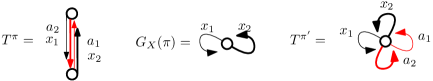
Figure 12. Left: A labeled graph $T^{\pi}$ for $\pi\in\mathcal{DU}^{opp}_{1,+}$. Middle: the graph $G^{\pi}_{X}$. Right a labeled graph $T^{\pi^{\prime}}$ for $\pi^{\prime}\in\mathcal{DU}^{opp}_{1,-}$ such that $G^{\pi}_{X}=G_{X}^{\pi^{\prime}}$.

We denote by $\mathcal{T}^{(1)}$ the set of partitions $\pi$ of $V$ such that the double cycle of $\mathcal{GDC}(T^{\pi})$ is of length 1, i.e. it is a self-loop labeled by a Wigner matrix. In this situation,

$$\omega(\pi)=\mathrm{E}[{x^{(\pi)}_{11}}^{2}],$$

where $X^{(\pi)}=\big{(}\frac{x_{ij}^{(\pi)}}{\sqrt{N}}\big{)}$ denotes the Wigner matrix associated to the through string. If $\pi\in\mathcal{DU}^{opp}\setminus\mathcal{T}^{(1)}$, then $\omega(\pi)=1$ and if $\pi\in\mathcal{DU}^{par}\setminus\mathcal{T}^{(1)}$ then $\omega(\pi)=\theta(\pi)$ defined in (38) as before.

Let $G\in\mathcal{G}^{par}_{2\ell+1}\cup\mathcal{G}^{opp}_{2\ell+1}$ for $\ell\geq 1$. There is no modification of the reasoning, compare to the even moments case, and we get

$$\sum_{G\in\mathcal{G}^{opp}_{2\ell+1}}\sum_{\begin{subarray}{c}\pi\in\mathcal{DU}^{opp}_{2\ell+1}\\ \mathrm{s.t.\ }G^{\pi}_{X}=G\end{subarray}}\prod_{C\in C_{A}}\frac{1}{N}\mathrm{Tr}^{0}[C]$$

$$\underset{N\rightarrow\infty}{\longrightarrow} \sum_{\sigma\in NC^{(2\ell+1)}(m,n)}\varphi_{K(\sigma)}(a_{1},\dots,a_{m+n})$$

$$\sum_{G\in\mathcal{G}^{par}_{2\ell+1}}\sum_{\begin{subarray}{c}\pi\in\mathcal{DU}^{par}_{2\ell+1}\\ \mathrm{s.t.\ }G^{\pi}_{X}=G\end{subarray}}\theta(G)\prod_{C\in C_{A}}\frac{1}{N}\mathrm{Tr}^{0}[C]$$

$$\underset{N\rightarrow\infty}{\longrightarrow} \sum_{\sigma\in NC^{(2\ell+1)}(m,n)}\theta_{\sigma}\varphi_{K(\sigma)}(a_{1},\dots,a_{m},a_{m+n}^{t},\dots,a_{m+1}^{t}).$$

We denote by $\mathcal{DU}^{opp}_{1,+}$ the set of $\pi\in\mathcal{DU}^{opp}_{1}$ (opposite type partitions with a single Wigner matrix on the double cycle) but the double cycle is not of length one, and $\mathcal{DU}^{opp}_{1,-}=\mathcal{DU}^{opp}_{1}\setminus\mathcal{DU}^{opp}_{1,+}$. For $\pi\in\mathcal{DU}^{opp}_{1,+}$, the graph $G^{\pi}_{X}$ is degenerated in the sense that it as a double self-loop. Given $G\in\mathcal{G}^{opp}_{1}$, all graphs $\pi\in\mathcal{DU}^{opp}_{1,+}$ such that $G^{\pi}_{X}=G$ have same graph $G^{\pi}_{A}$, which is a disjoint union of simple cycles $C_{1},\dots,C_{k}$. Similarly all graphs $\pi^{\prime}\in\mathcal{DU}^{opp}_{1,-}$ such that $G^{\pi}_{X}=G$ have same graph $G_{A}^{\pi^{\prime}}$, which is a disjoint union of simple cycles $\tilde{C}_{1},\dots,\tilde{C}_{k}$ where each $\tilde{C}_{i}$ is equal to $C_{i}$ but one $\tilde{C}_{i}$, obtained by identifying vertices of $C_{i}$. Hence we get

$$\tau^{(2)}_{con} \underset{N\rightarrow\infty}{\longrightarrow} \sum_{\begin{subarray}{c}\sigma\in NC_{2}(m,n)\\ \text{non-mixing}\end{subarray}}\varphi_{K(\sigma)}(a_{1},\dots,a_{m+n})$$

$$+\sum_{\begin{subarray}{c}\sigma\in NC_{2}(m,n)\\ \text{non-mixing}\end{subarray}}\theta_{\sigma}(\varphi_{(t)})_{K(\sigma)}(a_{1},\dots,a_{m+n})$$

$$+\sum_{\begin{subarray}{c}\sigma\in NC_{2}^{(1)}(m,n)\\ \text{non-mixing}\end{subarray}}(\eta_{\sigma}-1-\theta_{\sigma})\tilde{\varphi}_{K(\sigma)}(a_{1},\dots,a_{m+n}).$$

This is the formula (6) as claimed in Theorem 6, if we take also into account that the term from (6) involving $k_{4}$ is not showing up in the present case where both $m$ and $n$ are odd.

This finishes the proof of both Theorem 5 and Theorem 6.

M

References

- [1] Greg Anderson, Ofer Zeitouni, and Alice Guionnet, An introduction to random matrices. Cambridge University Press, 2010.
- [2] Benson Au, Guillaume Cébron, Antoine Dahlqvist, Franck Gabriel, and Camille Male, Freeness over the Diagonal for Large Random Matrices. To appear in Ann. Probab., arXiv:1805.07045
- [3] A. Boutet de Monvel and A. Khorunzhy., Asymptotic distribution of smoothed eigenvalue density. I. Gaussian random matrices. Random Oper. Stochastic Equations, 7(1):1-22, 1999
- [4] Dallaporta, Sandrine and Février, Maxime, Fluctuations of linear spectral statistics of deformed Wigner matrices. RMTA (9) 31–60.
- [5] K. Dykema, On certain free product factors via an extended matrix model. J. Funct. Anal., 112, 1993, 31-60.
- [6] Franck Gabriel, Holonomy fields and random matrices: invariance by braids and permutations Doctoral dissertation, 2016, HAL databas id: tel-01495593.
- [7] Alice Guionnet, Large Random Matrices: Lectures on Macroscopic Asymptotics. Saint-Flour’s summer school XXXVI 2006.
- [8] Ji, Hong Chang and Lee, Ji Oon, Gaussian fluctuations for linear spectral statistics of deformed Wigner matrices. RMTA (09) 2050011.
- [9] Kurt Johansson, On the fluctuations of eigenvalues of random Hermitian matrices. Duke Math. J. 91 1998, 151-204.
- [10] Dag Jonsson, Some limit theorems for the eigenvalues of a sample second-order distribution matrix. J. Mult. Anal. 12, 1982, 1-38.
- [11] A. M. Khorunzhy, B. A. Khoruzhenko, and L. A. Pastur, Asymptotic properties of large random matrices with independent entries. J. Math. Phys. 37 (1996) 5033-5060.
- [12] Camille Male, The limiting distributions of heavy Wigner and arbitrary random matrices. JFA, 2017.
- [13] Camille Male, Traffic distributions and independence: permutation invariant random matrices and the three notions of independence. Memoir AMS, to be published around 2020.
- [14] Camille Male, Forte et fausse libertés asymptotiques de grandes matrices aléatoires Doctoral dissertation, 2011, HAL databas id: tel-00673551.
- [15] James Mingo and Alexandru Nica, Annular non-crossing permutations and partitions, and second-order asymptotics for random matrices. Int. Math. Res. Not. 28 (2004) 1413-1460.
- [16] James Mingo and Roland Speicher, Second order freeness and fluctuations of random matrices. I. Gaussian and Wishart matrices and cyclic Fock spaces. J. Funct. Anal. 235 (2006), no. 1, 226-270.
- [17] James Mingo and Roland Speicher, Sharp bounds for sums associated to graph of matrices. J. Funct. Anal. 2011.
- [18] James Mingo and Roland Speicher, Free probability and random matrices. Fields Institute Monographs, Vol. 35, Springer, 2017.
- [19] Alexandru Nica and Roland Speicher, Lectures on the Combinatorics of Free Probability. Cambridge University Press, 2006.
- [20] E. Redelmeier, Real Second-Order Freeness and the Asymptotic Real Second-Order Freeness of Several Real Matrix Models. Int. Math. Res. Not. 2014 (12).
- [21] M. Shcherbina, Central Limit Theorem for linear eigenvalue statistics of the Wigner and sample covariance random matrices. J. Math. Phys., Analysis,Geometry, 7, 2011.
- [22] Mariya Shcherbina. Fluctuations of linear eigenvalue statistics of matrix models in the multi-cut regime. Journal of Statistical Physics, 151(6):1004-1034, 2013.
- [23] Y. Sinai and A. Soshnikov, Central limit theorem for traces of large random symmetric matrices with independent matrix elements. Bol. Soc. Brasil. Mat. (N.S.), 29, 1998, 1-24.
- [24] A. Soshnikov. The central limit theorem for local linear statistics in classical compact groups and related combinatorial identities. Ann. Probab.,28 (3): 1353-1370, 2000.
- [25] Dan Voiculescu, Limit laws for Random matrices and free products. Inventiones mathematicae December 1991, Volume 104, Issue 1, pp 201-220.
- [26] Dan Voiculescu, A strengthened asymptotic freenes result for random matrices with applications to free entropy. Int. Math. Res. Not. 1998 (1).
- [27] Eugene P. Wigner, On the distribution of the roots of certain symmetric matrices. Annals Math. , 67, 1958, 325-327.