Learning effective physical laws for generating cosmological hydrodynamics with Lagrangian Deep Learning

Abstract

The goal of generative models is to learn the intricate relations between the data to create new simulated data, but current approaches fail in very high dimensions. When the true data generating process is based on physical processes these impose symmetries and constraints, and the generative model can be created by learning an effective description of the underlying physics, which enables scaling of the generative model to very high dimensions. In this work we propose Lagrangian Deep Learning (LDL) for this purpose, applying it to learn outputs of cosmological hydrodynamical simulations. The model uses layers of Lagrangian displacements of particles describing the observables to learn the effective physical laws. The displacements are modeled as the gradient of an effective potential, which explicitly satisfies the translational and rotational invariance. The total number of learned parameters is only of order 10, and they can be viewed as effective theory parameters. We combine N-body solver FastPM with LDL and apply them to a wide range of cosmological outputs, from the dark matter to the stellar maps, gas density and temperature. The computational cost of LDL is nearly four orders of magnitude lower than the full hydrodynamical simulations, yet it outperforms it at the same resolution. We achieve this with only of order 10 layers from the initial conditions to the final output, in contrast to typical cosmological simulations with thousands of time steps. This opens up the possibility of analyzing cosmological observations entirely within this framework, without the need for large dark-matter simulations.

Keywords deep learning  $\cdot$ Lagrangian approach  $\cdot$ cosmological hydrodynamical simulation

1 Introduction

Numerical simulations of large scale structure formation in the universe are essential for extracting cosmological information from the observations [1, 2, 3, 4, 5, 6, 7]. In principle hydrodynamical simulations are capable of predicting the distribution of all observables in the universe, and thus can model observations directly. However, running high resolution hydrodynamical simulations at volumes comparable to the current and future sky surveys is currently not feasible, due to its high computational costs. The most widely used method is running gravity-only N-body simulations, and then populating baryons in the halo catalogs with semi-analytical approaches such as halo occupation distribution (HOD) [8], or halo assembly models [9]. However, these methods make strong assumptions such as the halo mass being the main quantity controlling the baryonic properties. In addition, many of the cosmological observations such as X-ray emission and Sunyaev-Zeldovich emission are based on hydrodynamic gas properties such as gas density, temperature, pressure etc., which cannot be modeled in the dark matter only simulations.

Deep learning methods provide an alternative way to model the cosmological observables. A number of papers view the task as an image-to-image translation problem, i.e., they take in pixelized matter density field as input data, and output the target pixelized observable field. These methods either model the conditional probability distribution $p(y_{\mathrm{t}arget}|x_{\mathrm{i}nput})$ using deep generative models such as GANs [10] and VAEs [11, 12], or learn a mapping $x_{\mathrm{i}nput}\mapsto y_{\mathrm{t}arget}$ with deep convolutional neural networks (DCNN). Previous work in this area covers a wide array of tasks, such as identifying halos (protohalos) [13, 14, 15, 16], producing 3D galaxy distribution [17], generating tSZ signals [18], predicting dark matter annihilation feedback [19], learning neutrino effects [20], emulating high resolution features from low resolution simulations [21] etc.

Unlike these methods that work in pixel (Eulerian) space and treat the field as images, another way to model the dynamics is to adopt the Lagrangian scheme, i.e., trace the motion of individual particles or fluid elements by modeling their displacement field. The displacement field contains more information than the density field, as different displacement fields can produce the same density field, and is in general more Gaussian and linear than the density field. Existing methods in this space only cover the dark matter, e.g. approximate N-body solvers [22, 23] and DCNN [24].

In this work we propose a novel deep learning architecture, Lagrangian Deep Learning (LDL), for modeling both the cosmological dark matter and the hydrodynamics, using the Lagrangian approach. The model is motivated by the effective theory ideas in physics, where one describes the true process, which may be too complicated to model, with an effective, often coarse grained, description of physics. A typical example is the effective field theory, where perturbative field theory is supplemented with an effective field theory terms that obey the symmetries, and are an effective coarse-grained description of the non-perturbative small scale effects. The resulting effective description has a similar structure as the true physics, but with free coefficients that one must fit for, and that account for the non-perturbative small scale effects.

Lagrangian Deep Learning

A cosmological dark matter and baryon evolution can be described by a system of partial differential equations (PDE) coupling gravity, hydrodynamics, and various sub-grid physics modeling processes such as the star formation, which are evolved in time from the beginning of the universe until today. One would like to simulate a significant fraction of the observable universe, while also capturing important physical processes on orders of magnitude smaller scales, all in three dimensions. As a result the resulting dynamical range is excessive even for the modern computational platforms. As an example, the state of the art Illustris TNG300-1 [25, 26, 27, 28, 29] has of order $10^{10}$ particles, yet simulates only a very small fraction of observable universe. The lower resolution TNG300-3 reduces the number of particles by 64, at a cost of significantly reducing the realism of the simulation.

An effective physics approach is to rewrite the full problem into a large scale problem that we can solve, together with an effective description of the small scales which we cannot resolve. In theoretical physics this is typically done by rewriting the Lagrangian such that it takes the most general form that satisfy the symmetries of the problem, with free coefficients describing the effect of the small scale coarse-graining. In cosmology the large scale evolution is governed by gravity, which can easily be solved perturbatively or numerically. Effective descriptions using perturbative expansions exist [30], but fail to model small scales and complicated baryonic processes at the map level. While spatial coarse graining is the most popular implementation of this idea, one can also apply it to temporal coarse graining as well. A typical PDE solver requires many time steps, which is expensive. Temporal coarse graining replaces this with fewer integration time steps, at a price of replacing the true physics equations with their effective description, while ensuring the true solution on large scales, where the solution is known [22, 23].

Here we take this effective physics description idea and combine it with the deep learning paradigm, where one maps the data through several layers consisting of simple operations, and trains the coefficients of these layers on some loss function of choice. While machine learning layers are described with neural networks with a very large number of coefficients, here we will view a single layer as a single time step PDE solver, using a similar structure as the true physical laws. This has the advantage that it can preserve the symmetries inherent in the problem. The main symmetry we wish to preserve in a cosmological setting is the translational and rotational symmetry: the physical laws have no preferred position or direction. But we also wish to satisfy the existing conservation laws, such as the dark matter and baryon mass conservation.

A very simple implementation of these two requirements is Lagrangian displacements of particles describing the dark matter or baryons. We displace the particles using the gradient of a potential, and mass conservation is ensured since we only move the particles around. To ensure the translation and rotation symmetry within the effective description we shape the potential in Fourier space, such that it only depends on the amplitude of the Fourier wave vector. The potential gradient can be viewed as a force acting upon their acceleration via the Newton’s law, and the shaping of the potential is equivalent to the radial dependence of the force. This description requires particle positions and velocities, so it is a second order PDE in time. We will use this description for the dark matter. However, for baryons we can simplify the modeling by assuming their velocity is the same as that of the dark matter, since velocity is dominated by large scales where the two trace each other. In this case we can use the potential gradient to displace particle positions directly, so the description becomes effectively first order in time. Moreover, by a simple extension of the model we can apply this concept to the baryonic observables such as the gas pressure and temperature, where conservation laws no longer apply. A complete description also requires us to define the source for the potential. In physics this is typically some property of the particles, such as mass or charge. Here we wish to describe the complicated nonlinear processes of subgrid physics, as well as coarse graining in space and time. Motivated by gravity we will make the simplest possible assumption of the source being a simple power law of the density, using a learned Green’s function to convert to the potential. Since we wish to model several different physics processes we stack it into multiple layers. Because the model takes in the particle data and models the displacement field from the Lagrangian approach using multiple layers, we call this model Lagrangian Deep Learning (LDL).

Our specific goal is to model the distribution of dark matter and hydrodynamic observables starting from the initial conditions as set in the early universe, using an effective description that captures the physics symmetries and conservation laws. An example of such a process applied to time and spatial coarse graining is the dark matter evolution with a few time steps only, which combines ideas such as the approximate N-body solvers, with a force sharpening process called the Potential Gradient Descent (PGD) to capture the coarse graining [31, 32]. We first use FastPM [23], a quasi particle-mesh (PM) N-body solver, which ensures the correct large scale growth at any number of time steps, since the kick and drift factors of the leapfrog integrator in FastPM are modified following the linear (Zel’dovich) equation of motion. FastPM has a few layers only (typically 5-10) and uses particle displacements. It is supplemented by one additional layer of PGD applied to position only to improve the dark matter distribution on small scales. All of the steps of this process are in the LDL form, so can be viewed as its initial layers. The resulting dark matter maps are shown in figure 1 and show an excellent agreement with the full N-body simulation of Illustris TNG, which is also confirmed by numerical comparisons presented in [31]. This application is not learning new physics, but is learning the effective physics description of both time and spatial coarse graining: instead of 1000+ time steps in a standard N-body simulation we use only 10, and instead of the full spatial resolution we will use a factor of 64 reduced mass resolution.

Here we wish to extend these ideas to the more complex and expensive problem of cosmological hydrodynamics, where we wish to learn its physics using an effective description. Baryons are dissipative and collisional, with many physical processes, such as cooling, radiation, star formation, gas shocks, turbulence etc. happening inside the highest density regions called dark matter halos. One can add displacements to the dark matter particles to simulate these hydrodynamic processes, such that the particles after the displacement have a similar distribution as the baryons. Enthalpy Gradient Descent (EGD) is an example of this idea [31]: one adds small scale displacement to the dark matter particles to improve the small-scales of the low resolution approximate simulations, and to model the baryonic feedback on the total matter distribution. Motivated by these methods, we propose to model this displacement field by

$$\mathbf{S}=\alpha\mathbf{\nabla}\mathbf{\hat{O}_{G}}f(\delta),$$ (1)

where $\alpha$ is a learnable parameter, $\delta$ is the matter overdensity as output by the initial layers (FastPM and LDL on dark matter layer), $f(\delta)$ is the source term and can be an arbitrary function of $\delta$. Here we choose it to be a power law

$$f(\delta)=(1+\delta)^{\gamma},$$ (2)

with $\gamma$ a learnable parameter. $\mathbf{\hat{O}_{G}}$ is the Green’s operator, and can be written explicitly as

$$\mathbf{\hat{O}_{G}}f(\delta)=\int G(\mathbf{x-x^{\prime}})f(\delta(\mathbf{x^{\prime}}))d\mathbf{x^{\prime}},$$ (3)

where $G(\mathbf{x-x^{\prime}})$ is the Green’s function and we have used $G(\mathbf{x,x^{\prime}})=G(\mathbf{x-x^{\prime}})$ due to translational symmetry. The convolution in above equation can be easily calculated in Fourier space as $\mathbf{\hat{O}_{G}}f(\delta)=G(\mathbf{k})f(\delta)$, and we further have $G(\mathbf{k})=G(k)$ because of the rotational symmetry of the system. Following the PGD model, we model $\mathbf{\hat{O}_{G}}$ in Fourier space as

$$\mathbf{\hat{O}_{G}}=\exp(-(k_{h}/k)^{2})\exp(-(k/k_{l})^{2})\ k^{n},$$ (4)

where $k_{h}$, $k_{l}$ and $n$ are additional learnable parameters. The high pass filter $\exp(-(k_{h}/k)^{2})$ prevents the large scale growth, since the baryonic physics that we are trying to model is an effective description of the small scale physics, while the large scales are correctly described by the linear perturbative solution enforced by FastPM. Together with the low pass filter $\exp(-(k/k_{l})^{2})$, which has the typical effective theory form, the operator $\mathbf{\hat{O}_{G}}$ is capable of learning the characteristic scale of the physics we are trying to model. Note that both the source $f(\delta)$ and the shape of $\mathbf{\hat{O}_{G}}$ characterizes the complex bayron and subgrid physics and cannot be derived from first principles. They can only be learned from high resolution hydrodynamical simulations. Equation 1 - 4 defines the displacement field of one Lagrangian layer. We can stack multiple such layers to form a deep learning model, where each layer takes the particle output from the previous layer (which determines $\delta$ in Equation 1) and adds additional displacements to the particles. Such a deep model will be able to learn more complex physics. The idea is that different layers can focus on different physics components, which will differ in terms of the scale dependence of the potential and its gradient, as well as in terms of the source density dependence.

Note that if we set $\alpha=4\pi G{\bar{\rho}}$, $\gamma=1$, $k_{h}=0$, $k_{l}=\infty$ and $n=-2$, then Equation 1 is exactly the gravitational force. However, unlike the true dynamics which is a second order equation in time, one for the displacement and one for the velocity/momentum, here we are trying to effectively mimic the missing baryonic physics and therefore bypass the momentum. We also allow all these parameters to vary in order to model the physics that is different from gravity.

The final output layer is modeled as a nonlinear transformation on the particle density field:

$$F(x)=\mathrm{ReLU}(b_{1}(1+\delta^{\prime}(x))^{\mu}-b_{0}),$$ (5)

where $F$ is the output target field, $\mathrm{ReLU}(x)$ is the rectified linear unit, which is zero if $x<0$ and $x$ otherwise, $\delta^{\prime}$ is the particle overdensity field after the displacement, and $b_{0}$, $b_{1}$ and $\mu$ are learnable parameters. This is motivated by the physics processes that cannot be modeled as a matter transport (i.e. displacement). In the example of stars, the Lagrangian displacement layers are designed to learn the effect of gas cooling and collapse. After these displacement layers, the particles are moved towards the halo center, where protogalaxies are formed and we expect star formation to happen in these dense regions. This star formation process will be modeled by Equation 5: the $\mathrm{ReLU}$ thresholding aims at selecting the high density regions where the star formation happens. Such thresholding is typical of a subgrid physics model: in the absence of this thresholding we would need to transport all of the particles out of the low density regions where the star formation does not happen, a process that does not have a corresponding physical model.

Table 1: The numerical parameters of LDL hybrid simulations, low resolution TNG300-3 and the target TNG300-1 hydrodynamical simulations

	FastPM + LDL	TNG300-3-Dark + LDL	TNG300-3	TNG300-1
$N_{\mathrm{particle}}$	$625^{3}$	$625^{3}$	$N_{\mathrm{DM}}=625^{3}$ $N_{\mathrm{gas}}=625^{3}$	$N_{\mathrm{DM}}=2500^{3}$ $N_{\mathrm{gas}}=2500^{3}$
Force / Mesh Resolution ($h^{-1}\mathrm{ckpc}$)	$164$ (FastPM)      $328$ (LDL)	$4.0$ (TNG-Dark)      $328$ (LDL)	$\epsilon_{\mathrm{DM,*}}=4.0$ $\epsilon_{\mathrm{gas}}=1.0$	$\epsilon_{\mathrm{DM,*}}=1.0$ $\epsilon_{\mathrm{gas}}=0.25$
Number of Time Steps / layers	$N_{\mathrm{FastPM}}=10$ $N_{\mathrm{LDL,*}}=4$	$N_{\mathrm{TNG}}=9201$ $N_{\mathrm{LDL,*}}=3$	$209,161$	$6,203,062$
CPU Time	$T_{\mathrm{IC}}=2.3\ \mathrm{h}$ $T_{\mathrm{FastPM}}=5.1\ \mathrm{h}$ $T_{\mathrm{LDL,*}}=0.4\ \mathrm{h}$	$T_{\mathrm{TNG}}=5.9\ \mathrm{kh}$ $T_{\mathrm{LDL,*}}=0.3\ \mathrm{h}$	$0.05\ \mathrm{Mh}$	$34.9\ \mathrm{Mh}$

• The LDL parameters for generating stellar mass. The architecture for other observables can be found in Table 2. The total CPU time for LDL is 7.8 hours, compared to $5\times 10^{4}$ for the full hydro TNG300-3. Despite this the LDL outperforms the full hydro at the same resolution in all of the outputs. In this paper we are primarily concerned with a proof of principle and both FastPM and LDL are run with Python. We expect the CPU time to be further reduced if running them with C.

In this work we use both FastPM and N-body simulations, combining them with LDL to predict the baryon observables from the linear density map. We consider modeling the stellar mass, kSZ signal, tSZ signal and X-ray at redshift $z=1$, $z=0.5$ and $z=0$. The dark matter particles are firstly evolved to these redshifts with FastPM, and then passed to the LDL networks for modeling the baryons. The parameters in LDL are optimized by matching the output with the target fields from TNG300-1 hydrodynamical simulation [25, 26, 27, 28, 29]. Since the kSZ signal is proportional to the electron momentum $n_{e}v_{z}$, the tSZ signal is proportional to the electron pressure $n_{e}T$, and the X-ray emissivity is approximately proportional to $n_{e}^{2}T^{0.5}$ (we only consider the bremsstrahlung effect and ignore the Gaunt factor), we will model these fields in the rest of this paper.

Apart from FastPM, we also consider combining LDL models with full N-body simulations. We take the particle data at redshift $z=1$, $z=0.5$ and $z=0$ from TNG300-3-Dark, a low resolution dark-matter-only run of the TNG300 series, and feed the particles to LDL models. In the next section we will compare the performance of these two hybrid simulations against the target high resolution hydrodynamical simulation.

We summarize the numerical parameters of these simulations in Table 1. We also list TNG300-3, the low resolution hydrodynamic run of TNG300. TNG300-3 has the resolution of our hybrid simulations, and is a natural reference to compare the performance of our models with. Note that the mass resolution, force / mesh resolution and time resolution of our hybrid simulations are significantly lower than the target simulation, and the N-body simulation and deep learning networks are also much cheaper to run compared to simulating hydrodynamics. As a result, the FastPM-based and N-body-based hybrid simulations are 7 and 4 orders of magnitudes cheaper than the target simulation, respectively. When comparing to TNG300-3, our hybrid simulations are still 4 and 1 orders of magnitudes cheaper, respectively, and we show that by being trained on the high resolution TNG300-1 our simulations are superior to TNG300-3, and comparable to TNG300-1.

Results

Figure 1: Visualization of slices of the simulations: the first row is the input linear density field. The 2nd, 4th, 6th, 8th and 10th rows are predictions of dark matter overdensity, stellar mass, electron momentum density $n_{e}v_{z}$ (kSZ signal), electron pressure $n_{e}T$ (tSZ signal) and $n_{e}^{2}T^{0.5}$ (X-ray signal) from our FastPM+LDL hybrid simulation, respectively. The 3rd, 5th, 7th, 9th and 11th rows are the corresponding target fields from TNG300-1 hydrodynamical simulation. The left panel, middel panel and right panel are from redshift $z=0$, $z=0.5$ and $z=1$, respectively. The slices are from a $90.2\times 90.2\times 32.8h^{-1}\mathrm{Mpc}$ sub-box of the test set.

We show in Figure 1 the visualization of slices of the input linear density field and the output dark matter of our FastPM-based hybrid simulation, as well as the target fields in hydrodynamical simulation. Visual agreement between the two is very good. The results are shown for the dark matter density, stellar mass density, electron momentum density $n_{e}v_{z}$, where $n_{e}$ is electron density and $v_{z}$ radial velocity, electron pressure $n_{e}T$, where $T$ is the gas temperature, and X-ray emission proportional to $n_{e}^{2}T^{0.5}$.

Power Spectrum

Figure 2: Comparison of the 3D power spectrum (top panel), transfer function (middle panel) and cross correlation coefficient (bottom panel) of the stellar mass overdensity. We compare the LDL hybrid simulations, TNG300-3 and the target TNG300-1 hydrodynamical simulation, at redshifts 0, 0.05 and 1.

Figure 3: Comparison of the 2D power spectrum (top panel), transfer function (middle panel) and cross correlation coefficient (bottom panel) of the electron momentum density $n_{e}v_{z}$ (proportional to kSZ signal) between the LDL hybrid simulations, TNG300-3 and the target TNG300-1 hydrodynamical simulation.

Figure 4: Comparison of the 2D power spectrum (top panel), transfer function (middle panel) and cross correlation coefficient (bottom panel) of the electron pressure $n_{e}T$ (proportional to tSZ signal) between the LDL hybrid simulations, TNG300-3 and the target TNG300-1 hydrodynamical simulation.

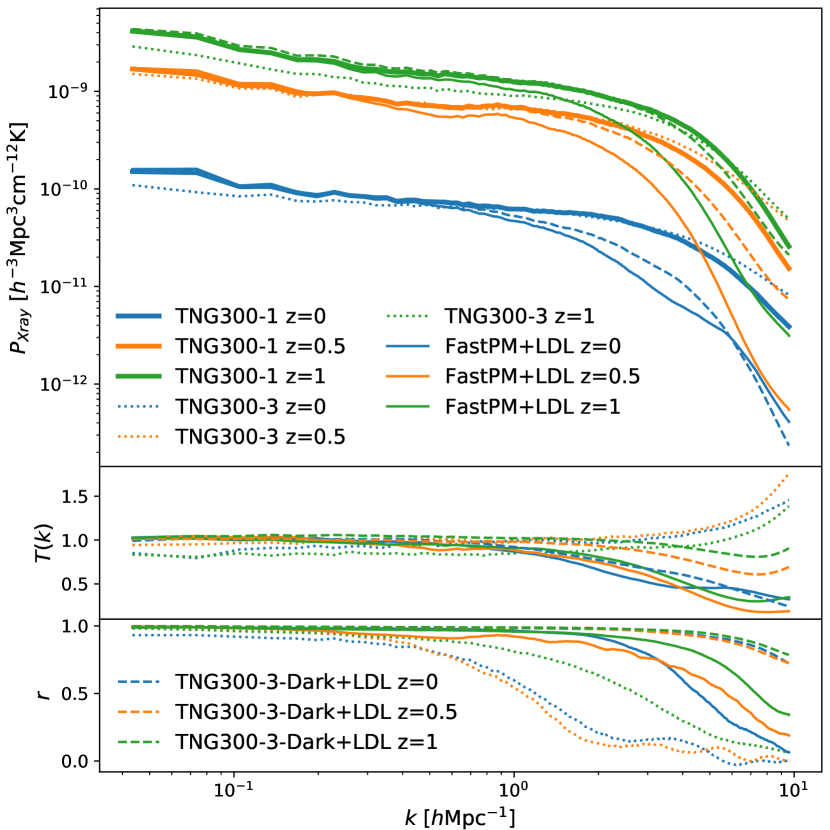
Figure 5: Comparison of the 3D power spectrum (top panel), transfer function (middle panel) and cross correlation coefficient (bottom panel) of the gas property $n_{e}^{2}T^{0.5}$ (proportional to X-ray emissivity) between the LDL hybrid simulations, TNG300-3 and the target TNG300-1 hydrodynamical simulation.

We measure the summary statistics of these fields and compare them quantitatively. We firstly compare the power spectrum, the most widely used summary statistics in cosmology. We define the transfer function as:

$$T(k)=\sqrt{\frac{P_{\mathrm{predict}}(k)}{P_{\mathrm{target}}(k)}},$$ (6)

and the cross correlation coefficient as:

$$r(k)=\frac{P_{\mathrm{predict,target}}(k)}{\sqrt{P_{\mathrm{predict}}(k)P_{\mathrm{target}}(k)}},$$ (7)

where $P_{\mathrm{predict,target}}(k)$ is the cross power spectrum between the predicted field and the target field. In this paper we use the whole $205h^{-1}\mathrm{Mpc}$ box for the measurement of power spectrum and cross correlations in order to compare the large scale modes. We show the 3D or 2D power spectrum, transfer function and cross correlation coefficient of the stellar mass overdensity $\delta_{*}$, electron momentum $n_{e}v_{z}$, electron pressure $n_{e}T$ and X-ray intensity $n_{e}^{2}T^{0.5}$ in Figures 2, 3, 4 and 5, respectively. On large scale and intermediate scale our hybrid simulations match well with the target fields, while TNG300-3 agreement is worse, especially for the stellar mass. The large bias of TNG300-3 stellar mass might be partially due to the fact that the low resolution TNG300-3 cannot resolve the stars in small halos. In contrast, by training on high resolution hydro simulations TNG300-1, our low resolution hybrid simulations are able to model those small galaxies better than the full hydro simulation at the same resolution.

On the small scales all of the predicted fields show some deviations from the targets. We discuss possible reasons for these in the next Section. We also see that the full-N-body-based hybrid simulation normally predicts larger small scale power than the FastPM-based simulation. This is likely due to the fact that the 10-layer FastPM cannot fully model the small halos and halo internal structures, and its simulated dark matter distribution is less clustered on small scale compared to full N-body simulations, making its predicted baryon fields less clustered. Overall, the predicted power spectrum from the N-body-based hybrid simulation is better, although it can predict too much small scale power (e.g. the kSZ signal at redshift 1).

The cross correlation coefficients are also shown in these Figures. We observe that the hybrid simulations are significantly better than those of TNG300-3, with the N-body-based hybrid simulation a bit higher than the FastPM-based simulation. Note that in principle the cross correlation coefficient, which quantifies the agreement of phases of Fourier modes, is a more important statistics than the transfer function, because the transfer function can always be corrected to unity by multiplying the predicted fields with the reciprocal of the transfer function. This again suggests that the baryon maps of our models are closer to the ground truth than full hydrodynamical simulations at the same resolution.

Cross Correlations between different tracers

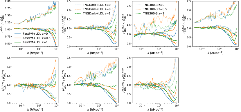
Figure 6: The ratio of the 2D cross power spectrum of different observables between the LDL hybrid simulations and the target TNG300-1 hydrodynamical simulation. The first row show the cross power spectrum of matter and stellar mass (1st panel), matter and tSZ signal (2nd panel), stellar momentum density and kSZ signal (3rd panel), and stellar mass and tSZ signal (4th panel). The second row shows the cross power spectrum of matter and X-ray (1st panel), stellar mass and X-ray (2nd panel), and tSZ and X-ray (3rd panel).

Probes of the large-scale structure, such as weak lensing, galaxy survey and clusters, are strongly correlated because they are all determined by the same underlying matter distribution. There is additional information in the cross correlations between these probes which cannot be obtained by analyzing each observable independently. The cross correlation also has the advantage that the noise does not add to it. Our hybrid simulation is able to generate various observables simultaneously with a low computational cost, so it is potentially promising for cross correlation analysis. Here we investigate the predicted cross correlations between weak lensing convergence, mass weighted galaxies, tSZ and X-ray, as well as the cross correlation between the galaxy momentum and kSZ signal. We show the ratio of the predicted cross power spectrum and the TNG300-1 in Figure 6. Similar to the auto power spectrum analysis, our predicted cross power spectrum is consistent with the target simulation on large scale, while TNG300-3 does not agree that well. On small scales FastPM-based hybrid simulation tends to underestimates the power, while TNG300-3 tends to overestimate the power. One can compare the second panel of Figure 6 (cross power spectrum between the matter and tSZ) with Figure 2 of [18], where GAN and VAE is used to predict the gas pressure from N-body simulations. We observe that the deviation of full-N-body-based hybrid simulation is comparable to the deviations of GAN and VAE. We note that for the standard deep learning architectures employed by GAN or VAE the number of parameters being fit is very large, in contrast to our approach.

Discussion

We propose a novel Lagrangian Deep Learning (LDL) model for learning the effective physical laws from the outputs of either simulations or real data. Specifically, in this paper we focus on learning the physics that controls baryon hydrodynamics in the cosmological simulations. We build hybrid simulations by combining N-body / quasi N-body gravity solver with LDL models. We show that both the FastPM-based and N-body-based hybrid simulations are able to generate maps of stellar mass, kSZ, tSZ and X-ray of various redshifts from the linear density field, and their computational costs are 7 and 4 orders of magnitudes lower than the target high resolution hydrodynamical simulation. We perform the auto power spectrum analysis and the cross correlation analysis among these fields, and we show that they outperform the hydrodynamical simulation at the same resolution.

The LDL model is motivated by the desire to provide an effective description of the underlying physics. Such a description must obey all the symmetries of the problem, and rotation and translation invariance are the two key symmetries, but other symmetries of the problem such as mass conservation may also appear. In this paper we argue that implementing these symmetries creates a generative model that is learning an effective description of the physical laws as opposed to learning the data distribution. This is because the symmetries are the only constraints on the generative model that must be implemented explicitly, everything else can be learned from the data. Here we propose that the learning of the generative model can be implemented by composing layers of displacements acting on the effective particles describing the physical properties of a system such as a fluid, moving the particles following the Lagrangian approach. The displacement of the particles can be understood as a result of the underlying physical processes, with particle transport a consequence of processes such as gas cooling and heating, feedback, turbulence etc. The output layer is a nonlinear transformation with thresholding on the particle density field, which models physics processes such as star formation.

Translational and rotational symmetry of the system put strong constraints on the model and therefore the Green’s operator can be written as a function in Fourier Space that only depends on the amplitude of $k$. This allows us to use very few parameters to model the complex processes and produce maps of observables. Thus even though we want to describe systems of extremely high dimensionality ($10^{8}$ or more), the underlying effective physics description requires a handful of parameters only.

The small number of free parameters also make the model stable and easy to train. An important advantage is that we can use the small number of parameters as effective physics description of a complicated microphysics model, similar to the free parameters that arise from renormalization in the effective field theory descriptions of microphysics. This suggests that our LDL approach can replace other effective descriptions used to model the process of star formation. In cosmology such simplified models are often based on first identifying the dark matter halos in a dark matter simulation only, followed by some effective description of how to populate these halos with stars. Compared to such semi-analytical approaches which often rely on non-differentiable models, our approach is explicitly differentiable, such that we can use backpropagation to derive a gradient of the final observables with respect to the initial density field. This can be easily embedded into the forward modeling framework to reconstruct the initial conditions from the observations [33].

Our current implementation outperforms the full hydro simulation at the same resolution, but does not match perfectly the higher resolution hydro simulation. LDL deviates from the full simulation results mostly on small scales. This is expected, since the factor of 64 lower mass resolution means there is some information in the full simulation that cannot be recovered. Specifically, we use a low resolution mesh for calculating the displacements in the LDL model (cell size $0.328h^{-1}\mathrm{Mpc}$, see Table 1). The low resolution mesh limits the ability of LDL to model the small scale baryon distribution. Moreover, to ensure the correct large scale distribution, we apply a smoothing operator (Equation 9) to the fields before calculating the loss function, which downweights the small scale contribution to the loss function.

LDL trains on hydrodynamic simulations and is not meant to replace but to complement them: for example, it can interpolate a coarse grid and scale them to larger volumes and higher resolutions. In contrast, LDL has the potential to eliminate the need for the semi-analytic methods, which are the current standard paradigm in the large scale structure. These methods run N-body simulations first and then populate their dark matter halos using a semi-analytic prescription for the observable. LDL can not only achieve results that are on par with the full hydro at the same resolution, which is superior to these semi-analytic approaches, it also achieves this with of order 10 time steps, in addition to up to 6 LDL layers, in contrast to $10^{3}$ in an N-body simulations. We expect this will lead both to development of realistic simulations that cover the full volume of the cosmological LSS surveys, and to analysis of these LSS surveys with LDL effective parameters as the nuisance parameters describing the astrophysics of the galaxy formation.

Dataset

IllustrisTNG is a suite of cosmological magneto-hydrodynamical simulations of galaxy formation and evolution [25, 26, 27, 28, 29]. It consists of three runs of different volumes and resolutions: TNG50, TNG100 and TNG300 with sidelengths of $35h^{-1}\mathrm{Mpc}\approx 50\mathrm{Mpc}$, $75h^{-1}\mathrm{Mpc}\approx 100\mathrm{Mpc}$ and $205h^{-1}\mathrm{Mpc}\approx 300\mathrm{Mpc}$, respectively. IllustrisTNG follows the evolution of the dark matter, gas, stars and supermassive black holes, with a full set of physical models including star formation and evolution, supernova feedback with galactic wind, primordial and metal-line gas cooling, chemical enrichment, black hole formation, growth and multi-mode feedback. The IllustrisTNG series evolves over a redshift range $z=127$ to the present $z=0$ in a $\mathrm{\Lambda CDM}$ cosmology, with parameters $\Omega_{m}=0.3089$, $\Omega_{b}=0.0486$, $\Omega_{\Lambda}=0.6911$, $H_{0}=67.74\mathrm{km\ s^{-1}\ Mpc^{-1}}$, $\sigma_{8}=0.8159$ and $n_{s}=0.9667$.

In this paper we train our models against TNG300-1, the highest resolution of the TNG300 run. TNG300-1 evolves $2500^{3}$ dark matter particles and an initial number of $2500^{3}$ gas cells, with a comoving force resolution $\epsilon_{\mathrm{DM,stars}}=1.0h^{-1}\mathrm{kpc}$, $\epsilon_{\mathrm{gas,min}}=0.25h^{-1}\mathrm{kpc}$ and $\epsilon_{\mathrm{BH,max}}=5.84h^{-1}\mathrm{kpc}$. The dark matter mass resolution is $4.0\times 10^{7}h^{-1}M_{\odot}$, and the target baryon mass resolution is $7.6\times 10^{6}h^{-1}M_{\odot}$ (see Table 1).

We also compare the model performance with TNG300-3, the hydro run with the same resolution as our hybrid simulations. The mass resolution and force resolution of TNG300-3 are 64 and 4 times lower than TNG300-1, respectively.

Details of the Hybrid Simulation

The 10-step FastPM is run in a $205h^{-1}\mathrm{Mpc}$ periodic box, but with only $N=625^{3}$ particles and force resolution $B=2$. We generate the initial condition at redshift $z=9$ using second order Lagrangian perturbation theory (2LPT), with the same random seed and linear power spectrum as Illustris-TNG. The linear density map is generated with a $N=1250^{3}$ mesh to improve the accuracy on small scale [32]. The box is then evolved to redshift $0$ with 10 time steps that are linearly separated in scale factor $a$. Three snapshots are produced at redshift $z=0$, $0.5$ and $1$, which are passed to LDL for generating maps of baryonic observables at these redshifts. Note that our mass, force and time resolutions are 64, 164 and 620,000 times lower than the target simulation TNG300-1, respectively.

Instead of running 10-step FastPM, we also tried using the particle data from the full N-body simulation TNG300-3-Dark. TNG300-3-Dark is the dark-matter-only run of the low resolution TNG300-3. It includes $N=625^{3}$ dark matter particles (same as our FastPM setup), but the force and time resolution is significantly higher. A detailed comparison between FastPM, TNG300-3-Dark and TNG300-1 can be found in Table 1.

Table 2: The LDL architecture for predicting different baryon observables

	stellar mass	kSZ		tSZ		X-ray
		$n_{e}$	$v_{z}$	$n_{e}$	$T$	$n_{e}$	$T$
Displacement Layer (Eq. 1)	2	1	0	1	2	2	2
Output Layer (Eq. 5)	1	1	0	1	1	1	1
Total number of layers	3 (4)	2 (3)		5 (6)		6 (7)
Total number of free parameters	13 (18)	10 (13)		21 (26)		26 (31)

• For FastPM-based hybrid simulation, we add one more displacement layer to improve the small scale dark matter distribution. The corresponding $N_{\mathrm{layer}}$ and $N_{\mathrm{parameter}}$ are shown in parentheses.

The details of the LDL model are described in the main text. We use a $N=625^{3}$ mesh for calculating the displacement and generating the hydro maps. The architecture of the model is shown in Table 2. Specifically, for FastPM input, we firstly add a Lagrangian displacement layer and the output is matched to the density field of the full N-body simulation TNG300-3-Dark. This layer is intended to improve the small scale structure of FastPM and is shared by all hydro outputs (we do not add this layer for TNG300-3-Dark input). Then for different observables, we train different displacement layers and output layer: 1. For stellar mass, we add two displacement layer to mimic gas cooling and collapse, and one output layer to model star formation. 2. For kSZ signal, we use one displacement layer and one output layer to model the electron number density field. We assume that the velocities of gas trace dark matter, so the velocity field can be directly estimated from the dark matter particles: $v(x)=\frac{p(x)}{\rho(x)}$, where $p(x)$ is the momentum density field and $\rho(x)$ is the matter density field. The kSZ map is obtained by multiplying the electron density field and the velocity field. 3. For tSZ signal map, we generate the electron number density field with one displacement layer and one output layer, and generate the gas temperature map with two displacement layers and one output layer. Then the two fields are multiplied to produce the tSZ signal. 4. The modeling of X-ray is similar to tSZ, except that now we use two displacement layer to model the electron density.

Model Training and Loss Function

As described above, the output of the LDL model is a $N=625^{3}$ mesh. We retain $77.7\%$ of the pixels for training, $13.8\%$ for validation and $8.5\%$ for test. Similar to [17], we split between training, validation, and test set following a “global” cut. The test set forms a sub-box of $90.2h^{-1}\mathrm{Mpc}$ per side, and the validation set is a $90.2\times 114.8\times 114.8\ h^{-1}\mathrm{Mpc}$ sub-box. The rest of the $205h^{-1}\mathrm{Mpc}$ box is used for training.

For stellar mass and the electron number density field in kSZ map, we define the loss function as:

$$\mathcal{L}=\sum_{i=1}^{N}\|\mathbf{\hat{O}_{s}}F_{\mathrm{LDL}}(x_{i})-\mathbf{\hat{O}_{s}}F_{\mathrm{TNG}}(x_{i})\|,$$ (8)

where $\|$ is $L_{2}$ norm, $i$ labels the mesh cell, $F_{\mathrm{LDL}}(x)$ is the generated map from LDL, $F_{\mathrm{TNG}}(x)$ is the true hydro map from IllustrisTNG, and $\mathbf{\hat{O}_{s}}$ is a smoothing operator defined in Fourier space:

$$\mathbf{\hat{O}_{s}}=1+(\frac{k}{1h\mathrm{Mpc^{-1}}})^{-n}.$$ (9)

Here $n$ is a hyperparameter that determines the relative weight between the large scale modes and the small scale modes. Without the $\mathbf{\hat{O}_{s}}$ operator, the model focuses on the small scale distribution and results in a biased large scale power due to the small number of large scale modes relative to small scale modes. We apply $\mathbf{\hat{O}_{s}}$ operator to put more weight on the large scale distribution. For most of the baryon maps we set $n=1$, except for the electron number density $n_{e}$ of the X-ray map we set it to be $n=0.85$.

For the tSZ map, we use a different loss function to improve the performance. We firstly train the electron density map with the following loss function:

$$\mathcal{L}_{n_{e}}^{\mathrm{tSZ}}=\sum_{i=1}^{N}\|\mathbf{\hat{O}_{s}}[n_{e_{\mathrm{LDL}}}(x_{i})T_{\mathrm{TNG}}(x_{i})]-\mathbf{\hat{O}_{s}}[n_{e_{\mathrm{TNG}}}(x_{i})T_{\mathrm{TNG}}(x_{i})]\|,$$ (10)

where $n_{e_{\mathrm{LDL}}}(x)$ is the learned electron number density map, $n_{e_{\mathrm{TNG}}}(x)$ is the true electron number density map, and $T_{\mathrm{TNG}}$ is the true temperature map. This means we multiply the electron number density field with the temperature field before calculating the loss function. This procedure puts more weight on the large clusters and improves the quality of the generated tSZ maps. Note that this electron density field is different from the electron density field for predicting the kSZ signal. Similarly, after we obtain the learned electron number density field $n_{e_{\mathrm{LDL}}}(x)$, we train the temperature map with the following the loss function:

$$\mathcal{L}_{T}^{\mathrm{tSZ}}=\sum_{i=1}^{N}\|\mathbf{\hat{O}_{s}}[n_{e_{\mathrm{LDL}}}(x_{i})T_{\mathrm{LDL}}(x_{i})]-\mathbf{\hat{O}_{s}}[n_{e_{\mathrm{TNG}}}(x_{i})T_{\mathrm{TNG}}(x_{i})]\|.$$ (11)

Here $n_{e_{\mathrm{LDL}}}(x)$ is the electron density field we just learned and is fixed, and $T_{\mathrm{LDL}}(x)$ is the target temperature field that we are trying to optimize.

For the X-ray map, similar to the tSZ signal, we train the electron density and gas temperature maps successively with the following loss functions:

$$\mathcal{L}_{n_{e}}^{\mathrm{X}}=\sum_{i=1}^{N}\|\mathbf{\hat{O}_{s}}[n^{2}_{e_{\mathrm{LDL}}}(x_{i})T^{0.5}_{\mathrm{TNG}}(x_{i})]-\mathbf{\hat{O}_{s}}[n^{2}_{e_{\mathrm{TNG}}}(x_{i})T^{0.5}_{\mathrm{TNG}}(x_{i})]\|,$$ (12)

$$\mathcal{L}_{T}^{\mathrm{X}}=\sum_{i=1}^{N}\|\mathbf{\hat{O}_{s}}[n^{2}_{e_{\mathrm{LDL}}}(x_{i})T^{0.5}_{\mathrm{LDL}}(x_{i})]-\mathbf{\hat{O}_{s}}[n^{2}_{e_{\mathrm{TNG}}}(x_{i})T^{0.5}_{\mathrm{TNG}}(x_{i})]\|.$$ (13)

Again, the electron number density field and gas temperature field for X-ray are different from the fields used for generating kSZ and tSZ.

Because the number of free parameters is relatively small, in this work we use the L-BFGS-B algorithm [34] for optimizing the model parameters.

References

- Eisenstein et al. [2011] Daniel J Eisenstein, David H Weinberg, Eric Agol, Hiroaki Aihara, Carlos Allende Prieto, Scott F Anderson, James A Arns, Éric Aubourg, Stephen Bailey, Eduardo Balbinot, et al. Sdss-iii: Massive spectroscopic surveys of the distant universe, the milky way, and extra-solar planetary systems. The Astronomical Journal, 142(3):72, 2011.
- Ivezic et al. [2009] Zeljko Ivezic, JA Tyson, T Axelrod, D Burke, CF Claver, KH Cook, SM Kahn, RH Lupton, DG Monet, PA Pinto, et al. Lsst: from science drivers to reference design and anticipated data products. In Bulletin of the American Astronomical Society, volume 41, page 366, 2009.
- Spergel et al. [2015] D Spergel, N Gehrels, C Baltay, D Bennett, J Breckinridge, M Donahue, A Dressler, BS Gaudi, T Greene, O Guyon, et al. Wide-field infrarred survey telescope-astrophysics focused telescope assets wfirst-afta 2015 report. arXiv preprint arXiv:1503.03757, 2015.
- Aghamousa et al. [2016] Amir Aghamousa, Jessica Aguilar, Steve Ahlen, Shadab Alam, Lori E Allen, Carlos Allende Prieto, James Annis, Stephen Bailey, Christophe Balland, Otger Ballester, et al. The desi experiment part i: Science, targeting, and survey design. arXiv preprint arXiv:1611.00036, 1611, 2016.
- Amendola et al. [2018] Luca Amendola, Stephen Appleby, Anastasios Avgoustidis, David Bacon, Tessa Baker, Marco Baldi, Nicola Bartolo, Alain Blanchard, Camille Bonvin, Stefano Borgani, et al. Cosmology and fundamental physics with the euclid satellite. Living reviews in relativity, 21(1):2, 2018.
- Springel et al. [2005] Volker Springel, Simon DM White, Adrian Jenkins, Carlos S Frenk, Naoki Yoshida, Liang Gao, Julio Navarro, Robert Thacker, Darren Croton, John Helly, et al. Simulations of the formation, evolution and clustering of galaxies and quasars. nature, 435(7042):629–636, 2005.
- DeRose et al. [2019] Joseph DeRose, Risa H Wechsler, Jeremy L Tinker, Matthew R Becker, Yao-Yuan Mao, Thomas McClintock, Sean McLaughlin, Eduardo Rozo, and Zhongxu Zhai. The aemulus project. i. numerical simulations for precision cosmology. The Astrophysical Journal, 875(1):69, 2019.
- Berlind and Weinberg [2002] Andreas A Berlind and David H Weinberg. The halo occupation distribution: Toward an empirical determination of the relation between galaxies and mass. The Astrophysical Journal, 575(2):587, 2002.
- Behroozi et al. [2019] Peter Behroozi, Risa H Wechsler, Andrew P Hearin, and Charlie Conroy. Universemachine: The correlation between galaxy growth and dark matter halo assembly from z= 0- 10. Monthly Notices of the Royal Astronomical Society, 488(3):3143–3194, 2019.
- Goodfellow et al. [2014] Ian Goodfellow, Jean Pouget-Abadie, Mehdi Mirza, Bing Xu, David Warde-Farley, Sherjil Ozair, Aaron Courville, and Yoshua Bengio. Generative adversarial nets. In Advances in neural information processing systems, pages 2672–2680, 2014.
- Kingma and Welling [2013] Diederik P Kingma and Max Welling. Auto-encoding variational bayes. arXiv preprint arXiv:1312.6114, 2013.
- Rezende et al. [2014] Danilo Jimenez Rezende, Shakir Mohamed, and Daan Wierstra. Stochastic backpropagation and approximate inference in deep generative models. arXiv preprint arXiv:1401.4082, 2014.
- Modi et al. [2018] Chirag Modi, Yu Feng, and Uroš Seljak. Cosmological reconstruction from galaxy light: neural network based light-matter connection. Journal of Cosmology and Astroparticle Physics, 2018(10):028, 2018.
- Berger and Stein [2019] Philippe Berger and George Stein. A volumetric deep convolutional neural network for simulation of mock dark matter halo catalogues. Monthly Notices of the Royal Astronomical Society, 482(3):2861–2871, 2019.
- Ramanah et al. [2019] Doogesh Kodi Ramanah, Tom Charnock, and Guilhem Lavaux. Painting halos from cosmic density fields of dark matter with physically motivated neural networks. Physical Review D, 100(4):043515, 2019.
- Bernardini et al. [2020] Mauro Bernardini, Lucio Mayer, Darren Reed, and Robert Feldmann. Predicting dark matter halo formation in n-body simulations with deep regression networks. Monthly Notices of the Royal Astronomical Society, 496(4):5116–5125, 2020.
- Zhang et al. [2019] Xinyue Zhang, Yanfang Wang, Wei Zhang, Yueqiu Sun, Siyu He, Gabriella Contardo, Francisco Villaescusa-Navarro, and Shirley Ho. From dark matter to galaxies with convolutional networks. arXiv preprint arXiv:1902.05965, 2019.
- Tröster et al. [2019] Tilman Tröster, Cameron Ferguson, Joachim Harnois-Déraps, and Ian G McCarthy. Painting with baryons: augmenting n-body simulations with gas using deep generative models. Monthly Notices of the Royal Astronomical Society: Letters, 487(1):L24–L29, 2019.
- List et al. [2019] Florian List, Ishaan Bhat, and Geraint F Lewis. A black box for dark sector physics: Predicting dark matter annihilation feedback with conditional gans. Monthly Notices of the Royal Astronomical Society, 490(3):3134–3143, 2019.
- Giusarma et al. [2019] Elena Giusarma, Mauricio Reyes Hurtado, Francisco Villaescusa-Navarro, Siyu He, Shirley Ho, and ChangHoon Hahn. Learning neutrino effects in cosmology with convolutional neural networks. arXiv preprint arXiv:1910.04255, 2019.
- Kodi Ramanah et al. [2020] Doogesh Kodi Ramanah, Tom Charnock, Francisco Villaescusa-Navarro, and Benjamin D Wandelt. Super-resolution emulator of cosmological simulations using deep physical models. Monthly Notices of the Royal Astronomical Society, 495(4):4227–4236, 2020.
- Tassev et al. [2013] Svetlin Tassev, Matias Zaldarriaga, and Daniel J Eisenstein. Solving large scale structure in ten easy steps with cola. Journal of Cosmology and Astroparticle Physics, 2013(06):036, 2013.
- Feng et al. [2016] Yu Feng, Man-Yat Chu, Uroš Seljak, and Patrick McDonald. Fastpm: a new scheme for fast simulations of dark matter and haloes. Monthly Notices of the Royal Astronomical Society, 463(3):2273–2286, 2016.
- He et al. [2019] Siyu He, Yin Li, Yu Feng, Shirley Ho, Siamak Ravanbakhsh, Wei Chen, and Barnabás Póczos. Learning to predict the cosmological structure formation. Proceedings of the National Academy of Sciences, 116(28):13825–13832, 2019.
- Pillepich et al. [2018] Annalisa Pillepich, Dylan Nelson, Lars Hernquist, Volker Springel, Rüdiger Pakmor, Paul Torrey, Rainer Weinberger, Shy Genel, Jill P Naiman, Federico Marinacci, et al. First results from the illustristng simulations: the stellar mass content of groups and clusters of galaxies. Monthly Notices of the Royal Astronomical Society, 475(1):648–675, 2018.
- Naiman et al. [2018] Jill P Naiman, Annalisa Pillepich, Volker Springel, Enrico Ramirez-Ruiz, Paul Torrey, Mark Vogelsberger, Rüdiger Pakmor, Dylan Nelson, Federico Marinacci, Lars Hernquist, et al. First results from the illustristng simulations: A tale of two elements–chemical evolution of magnesium and europium. Monthly Notices of the Royal Astronomical Society, 477(1):1206–1224, 2018.
- Marinacci et al. [2018] Federico Marinacci, Mark Vogelsberger, Rüdiger Pakmor, Paul Torrey, Volker Springel, Lars Hernquist, Dylan Nelson, Rainer Weinberger, Annalisa Pillepich, Jill Naiman, et al. First results from the illustristng simulations: radio haloes and magnetic fields. Monthly Notices of the Royal Astronomical Society, 480(4):5113–5139, 2018.
- Springel et al. [2018] Volker Springel, Rüdiger Pakmor, Annalisa Pillepich, Rainer Weinberger, Dylan Nelson, Lars Hernquist, Mark Vogelsberger, Shy Genel, Paul Torrey, Federico Marinacci, et al. First results from the illustristng simulations: matter and galaxy clustering. Monthly Notices of the Royal Astronomical Society, 475(1):676–698, 2018.
- Nelson et al. [2018] Dylan Nelson, Annalisa Pillepich, Volker Springel, Rainer Weinberger, Lars Hernquist, Rüdiger Pakmor, Shy Genel, Paul Torrey, Mark Vogelsberger, Guinevere Kauffmann, et al. First results from the illustristng simulations: the galaxy colour bimodality. Monthly Notices of the Royal Astronomical Society, 475(1):624–647, 2018.
- Carrasco et al. [2012] John Joseph M Carrasco, Mark P Hertzberg, and Leonardo Senatore. The effective field theory of cosmological large scale structures. Journal of High Energy Physics, 2012(9):82, 2012.
- Dai et al. [2018] Biwei Dai, Yu Feng, and Uroš Seljak. A gradient based method for modeling baryons and matter in halos of fast simulations. Journal of Cosmology and Astroparticle Physics, 2018(11):009, 2018.
- Dai et al. [2020] Biwei Dai, Yu Feng, Uroš Seljak, and Sukhdeep Singh. High mass and halo resolution from fast low resolution simulations. Journal of Cosmology and Astroparticle Physics, 2020(04):002, 2020.
- Seljak et al. [2017] Uroš Seljak, Grigor Aslanyan, Yu Feng, and Chirag Modi. Towards optimal extraction of cosmological information from nonlinear data. Journal of Cosmology and Astroparticle Physics, 2017(12):009, 2017.
- Byrd et al. [1995] Richard H Byrd, Peihuang Lu, Jorge Nocedal, and Ciyou Zhu. A limited memory algorithm for bound constrained optimization. SIAM Journal on scientific computing, 16(5):1190–1208, 1995.
- Hand et al. [2018] Nick Hand, Yu Feng, Florian Beutler, Yin Li, Chirag Modi, Uroš Seljak, and Zachary Slepian. nbodykit: An open-source, massively parallel toolkit for large-scale structure. The Astronomical Journal, 156(4):160, 2018.