A search for ultrahigh-energy neutrinos associated with astrophysical
sources using the third flight of ANITA

Abstract

The ANtarctic Impulsive Transient Antenna (ANITA) long-duration balloon experiment is sensitive to interactions of ultrahigh-energy ($E>10^{18}$ eV) neutrinos in the Antarctic ice sheet. The third flight of ANITA, lasting 22 days, began in December 2014. We develop a methodology to search for energetic neutrinos spatially and temporally coincident with potential source classes in ANITA data. This methodology is applied to several source classes: the potential IceCube-identified neutrino sources TXS 0506+056and NGC 1068, flaring high-energy blazars reported by the Fermi All-Sky Variability Analysis, gamma-ray bursts, and supernovae. Among searches within the five source classes, one candidate was identified as associated with SN 2015D, although not at a statistically significant level. We proceed to place upper limits on the source classes. We further comment on potential application of this methodology to more sensitive future instruments.

1 Introduction

The Antarctic Impulsive Transient Antenna (ANITA) experiment [1] deploys a balloon-borne radio interferometer to search for the impulsive Askaryan radio emission [2, 3] expected to be produced by the interactions of ultrahigh-energy (UHE) neutrinos ($E>10^{18}$ eV) interacting in polar ice. ANITA has previously reported constraints on diffuse UHE neutrinos [4, 5, 6, 7] as well as neutrinos in time-coincidence with gamma-ray bursts (GRBs) [8]. No candidate events have been observed above background expectations so far in the Askaryan channel, but ANITA sets the most stringent limits on diffuse UHE neutrino flux above $10^{19.5}$ eV.

Cosmogenic UHE neutrinos are expected to be produced in the interactions of the UHE cosmic-rays (UHECR) with the CMB (i.e. the GZK process) [9, 10, 11]. The sources of the UHECR have not yet been identified, and it is unknown if the sources are transient in nature or steady-state. Typical GZK interaction lengths of a few hundred Mpc imply cosmogenic neutrinos will retain the source direction over cosmological distances, but any time association with potential astrophysical transients is likely lost due to deflections of UHECR by intergalactic magnetic fields.

Astrophysical neutrinos, believed to be produced directly in astrophysical sources, have been detected at TeV-PeV energies by IceCube [12]. IceCube has identified evidence for some particular astrophysical neutrino sources, including TXS 0506+056 [13, 14] and NGC 1068 [15]. Astrophysical neutrinos may also exist at UHE energies, either as a continuation of the same flux that IceCube has detected, or from other sources, such as flat-spectrum radio quasars (FSRQs) [16, 17, 18] or GRBs [19, 20, 21, 22, 23].

Compared to a diffuse UHE neutrino search, a search for UHE neutrinos associated with particular sources can narrow the detection phase space in direction and, for transient objects, in time. This in general allows a reduction in backgrounds and/or an improvement in analysis efficiency, therefore increasing the sensitivity compared to diffuse fluxes.

In this paper, we build on an ANITA-III diffuse search to develop a methodology to search for UHE neutrinos in spatial and time coincidence with astrophysical source classes. We define a source class as a specification of the time-dependent neutrino flux from one or more sources, $\mathbf{F}(E,t)=\sum_{\rm{sources}}F_{i}(E,t)$. This methodology is applied to the ANITA-III flight for five source classes: TXS 0506+056, NGC 1068, blazars flaring in UHE gamma-rays as identified by the Fermi All-sky Variability Analysis (FAVA [24]), GRBs, and supernovae (SN).

2 Simulation

The standard ANITA simulation, icemc [25], is designed for efficient simulation of a diffuse flux of neutrinos. The volumetric sampling method used is efficient in sampling neutrinos likely to trigger ANITA, but is not appropriate for modeling point sources, as it relies on the “thin target” approximation, converting effective volume to effective area by dividing by the interaction length. As such, a specialized sampling scheme was developed for this search within icemc.

The first step is to choose a payload position/time and neutrino direction. A random time is chosen within the ANITA-III flight which determines the payload position and orientation. The neutrino direction is chosen based on the simulated parameters, for example, a single source, an isotropic flux, or from a collection of time-varying sources.

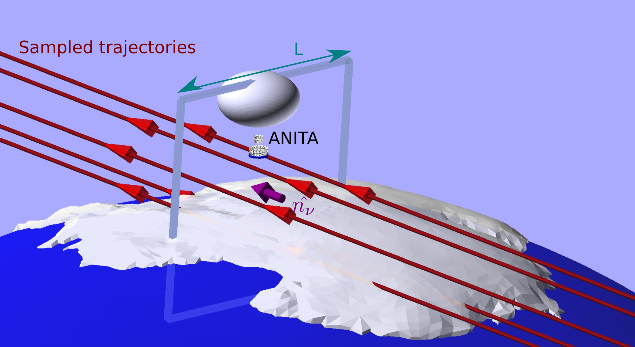
Figure 1: An illustration of the sampling method used for the point-source simulation. See text for details.

For a payload position, $\vec{x}_{\rm{ANITA}}$, and neutrino direction, $\hat{p}_{\nu}$, one straightforward way to calculate the effective area for a given neutrino energy, $E_{\nu}$, is to consider a square with side $L$, normal to $\hat{p}_{\nu}$ and uniformly select a point on the square to define the neutrino trajectory (see Figure  1). Assuming that the square is centered near $\vec{x}_{\rm{ANITA}}$ (we center it at the ice surface below ANITA) and $L$ is made large enough so all neutrinos that could trigger ANITA intersect the sampling square, the trigger-level effective area for that configuration is then:

$$A_{\rm{eff}}(\hat{p}_{\nu},\vec{x}_{\rm{ANITA}},E_{\nu})=L^{2}\frac{n_{\rm{trigger}}}{n_{\rm{thrown}}}.$$ (2.1)

A value of $L=1200$ km is a conservative choice that will miss no triggered neutrinos for ANITA-III.

This scheme can be generalized to calculate ANITA’s effective area to a point source with sky position $\Theta$ by choosing the appropriate $\hat{p}_{\nu}$ at each sampled $\vec{x}_{\rm{ANITA}}$, integrating over the flight trajectory by uniformly choosing random times within the flight:

$$A_{\rm{eff}}(\Theta,E_{\nu})=L^{2}\frac{n_{\rm{trigger}}}{n_{\rm{thrown}}}.$$ (2.2)

Mean ANITA-III trigger-level point-source effective area

Equatorial	Local

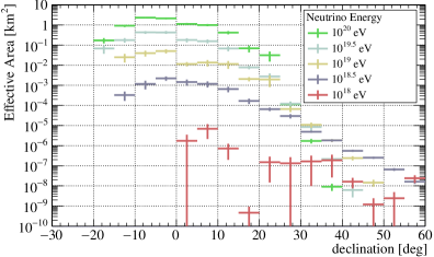
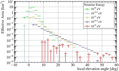
Figure 2: The point-source effective area as a function of declination (left) or local elevation angle (right) averaged over the ANITA-III flight at several energies. Local elevation angle is measured downward from payload horizontal. Because ANITA moves slowly compared to the diurnal cycle, the flight-averaged acceptance is nearly constant with right ascension. The total flight time is 22 days. Errors shown are statistical only (systematic uncertainties are estimated to be of order 50%). The point-source simulation results shown here are not directly comparable to the diffuse sensitivities quoted elsewhere by ANITA, as those diffuse sensitivities are geometric averages of ANITA’s diffuse acceptance given by two independent simulation codes.

The remaining task is to calculate $n_{\rm{trigger}}$. The obvious forward calculation—propagating a neutrino through the Earth until it interacts or exits and then checking if ANITA would have triggered on interacting neutrinos—requires a lot of computing time to acquire a sufficient sample of triggering neutrinos. To speed up calculation, we use the following scheme to calculate whether or not a given neutrino triggers ANITA:

1. Check if the neutrino trajectory intersects an ellipsoid 5 km bigger than the geodesic reference ellipsoid (the highest altitude in Antarctica is 4,892 m). If not, there is no chance of detection, so skip to the next event.

2. Find the intersection points of the neutrino with the Antarctic ice volume, which we take from BEDMAP2 [26]). A step size of 50 m is used in order to detect intersections with ice at least that small. If no intersection with ice is detected, then there is no chance of detecting this neutrino, so skip to the next event.

3. A trajectory may have multiple intersections with the ice. For each intersecting segment, we calculate a weight, $w_{s}$, that is the product of the probability of the neutrino interacting within ice segment and the probability that the neutrino did not interact in the Earth prior to reaching the segment.

4. We choose one intersecting segment at random and pick an interaction point within that segment exponentially distributed from the entry point according to the cross-section. We correspondingly multiply $w_{s}$ by the number of intersecting segments to compensate for the selection.

5. We then proceed with the rest of the simulation as implemented in icemc (pick interaction type from differential cross-section, sample inelasticity, etc.) and evaluate if ANITA triggers on the radio emission.

6. $n_{\rm{trigger}}$ is the sum of $w_{s}$ for events that trigger.

This method can also be used to simulate a diffuse flux by choosing the source direction at random in each trial, effectively integrating over $d\Omega$. By doing so, we can compare to the traditional icemc sampling method and find that the diffuse effective areas agree for ANITA-III at the 20% level, which we consider an acceptable level of agreement, subdominant to other systematic errors in the simulation of order 50% [25]. The time-averaged point-source UHE neutrino effective areas as a function of declination and elevation angles over the ANITA-III flight are shown in Figure 2.

Finally, this method may be adapted to simulate ANITA’s response to a source class. We integrate over the flight trajectory by sampling times during the flight. At each time, we draw from the sources active at the time with probability proportional to its relative flux compared to all other active sources and apply an additional time-dependent weight $w_{t}=\mathbf{F}(E,t)/\int_{t_{0}}^{t_{1}}\mathbf{F}(E,t)dt$.

3 Source Search Methodology

We adapt Analysis B from the ANITA-III diffuse search, which is described in detail in the appendices of [6]. A brief review is provided here.

3.1 Review of diffuse ANITA analysis

The ANITA payload consists of 48 dual-polarization horn antennas sensitive to a frequency range of approximately 200-1200 MHz. Whenever ANITA triggers, an event is formed from 96 100-ns-long waveforms digitized from 48 dual-polarization antennas with known relative positions and time delays. These waveforms are filtered to remove narrow-band contamination, then an interferometric map is generated for each polarization, where the mean cross-correlation between antennas is computed as a function of elevation and azimuth in payload-centric coordinates. Directions corresponding to the peaks of these maps are considered plane-wave source hypotheses and coherently-summed waveforms are created in those directions, from which various observables are computed. Analysis B applies three sets of cuts to select diffuse neutrino and air shower candidates:

1. Quality Cuts $(\mathcal{Q})$, to remove digitizer glitches, radio interference from the payload itself, and other problematic pathologies.

2. A Fisher discriminant, $(\mathcal{F}$), selecting for neutrino-like events. This multivariate discriminant is constructed using a variety of observables from event waveforms (e.g. cross-correlation, coherence, signal size, impulsivity, linear polarization) and is trained on a sideband of thermal events and simulation, to select impulsive broadband events.

3. A spatial isolation parameter, $\mathcal{O}$, based on projecting events to the continent, to remove likely anthropogenic events. This parameter is equal to the overlap integral of each event’s pointing resolution projected onto the continent with that of other events. Only events with sufficiently high $\mathcal{F}$ are included in this integral, with a soft turn-on (so that events less likely to be neutrino-like are given a smaller weight). As $\mathcal{O}$ quickly becomes very small for events that are far apart, it is convenient to set cuts on $-\log_{10}\mathcal{O}$ instead of $\mathcal{O}$ directly.

Emission from neutrinos at the payload is typically vertically-polarized due to the usual skimming geometry of UHE neutrinos and preferential transmission at the ice-air interface. Conversely, radio emission from extensive air showers produce impulsive signals that are predominantly horizontally-polarized [27]. To avoid this background, only predominantly vertically-polarized events are considered Askaryan neutrino candidates. $\mathcal{Q}$ was optimized to reduce the number of poor-quality events to a negligible level and then $\mathcal{F}$ and $\mathcal{O}$ each had cut values optimized for sensitivity to a diffuse flux. The primary contribution to the background estimate is anthropogenic, with negligible background from thermal noise, glitches, and payload-generated radio interference.

3.2 $\mathcal{D}$, the source class distance

Figure 3: The distribution in equatorial coordinates of the apparent RF direction (left) for simulated neutrinos from TXS 0506+056, and the proxy sky position(right) computed using the approximate reconstruction method described in the text. The more compact distribution allows for improved background discrimination. The color axis depicts the percentage of spatial distribution within each angular bin ($1^{\circ}\times 1^{\circ}$); bins contributing less than 0.01 percent are not shown for clarity. As one measure of the improvement in localization, the standard deviation in $\alpha$ improves from 13.3 degrees to 4.5 degrees and the standard deviation in $\delta$ improves from 6.4 degrees to 1.7 degrees.

We now develop a methodology to optimize the search for sensitivity to a given source class rather than a diffuse flux. The approach developed here strays from the well-established likelihood-based methodology employed, for example, in source searches by IceCube Observatory [15]. That technique, where a signal and background model are constructed and a likelihood analysis is performed scanning over possible signal models, does not translate straightforwardly to ANITA. The primary backgrounds to neutrino searches in ANITA are not “physical backgrounds” but instead anthropogenic radio emission. We don’t know how to model this background and so cannot easily incorporate it into a likelihood analysis (we rely on sidebands outside of the signal region to estimate it). Moreover, we wish to recycle most of the work from the diffuse search, which did not use a likelihood-based methodology.

For expedience, we will keep the definitions of $\mathcal{Q}$, $\mathcal{O}$, and $\mathcal{F}$ the same as in the diffuse search, but introduce a new “source distance” parameter, $\mathcal{D}$ (to be defined shortly), that is a measure of how closely-associated an event is to a source class. We will then optimize cut values for $\mathcal{F}$, $\mathcal{O}$ and $\mathcal{D}$ to maximize search sensitivity for each source class. The $\mathcal{Q}$ cut values are kept the same as in the diffuse analysis.

The interferometric event reconstruction used by ANITA produces an estimated direction of the radio emission ($\phi_{RF}$, $\theta_{RF}$) relative to the payload. Since the orientation, time, and position of the payload at each event are known, this direction may be projected into equatorial coordinates, right ascension ($\alpha$) and declination ($\delta$). Using simulation, the distributions of $(\alpha_{RF},\delta_{RF}$) may be estimated for a particular neutrino flux. However, due to the opening angle of the in-ice emission cone, these distributions are not compact for a single neutrino direction (see Figure 3, left). In order to efficiently select neutrinos from a direction, large swaths of the sky must be accepted, leading to a relatively higher amount of background. As such, we desire an observable related to neutrino direction that is more compact, which will tend to have higher background rejection for a given signal efficiency.

Reconstructing the neutrino direction for an event, rather than the direction of radio emission, would meet this goal. Because Askaryan emission is radially-polarized, the observed polarization state of the radio emission from neutrino is related to the neutrino direction. Similarly, the power spectral density of an event is related to how far away the emission angle is from the Cherenkov angle [28]. However, these observables are muddled by instrumental and radio propagation effects, and moreover, the highly-varying differential directional acceptance to neutrinos must be taken into account.

For a putative ANITA neutrino candidate, a straightforward (but dependent, as an energy spectrum must be assumed) way of estimating the neutrino direction is to simulate neutrinos from different directions with the payload fixed at the observation location in order to determine the neutrino directions compatible with observables. While this exercise would be worthwhile for a sufficiently-interesting candidate and would result in a compactly-defined unbiased neutrino direction distribution, it would be infeasible to perform this procedure on the many events considered in a search.

Fortunately, for our purposes, we can live with an approximate reconstruction of the neutrino direction, as any imperfections or biases would manifest themselves in both data and simulation. To this end, we derive a data-driven approximate reconstruction using machine learning techniques. A large set of isotropically-distributed neutrinos were simulated at various energies and run through the same reconstruction framework as data.

TMVA [29] was used to regress a polynomial for each of $\Delta\phi=\phi_{\nu}-\phi_{RF}$ and $\Delta\theta=\theta_{\nu}-\theta_{RF}$ as a function of a number of observables derived from the waveforms that appeared to be related to the relative neutrino direction. Fig. 4 (left) shows, as an example, the relationship between the reconstructed polarization angle and $\Delta\phi$ for the training dataset.

The polynomials used were lightly hand-tuned until acceptable results were produced. Further tuning or more sophisticated machine learning techniques could potentially yield even better results. The polynomials regressed were

$$\Delta\phi=P_{5}(\theta_{pol})+P_{1}(\theta_{RF})$$ (3.1)

and

$$\Delta\theta=P_{5}(\theta_{pol})+P_{1}(\theta_{RF})+P_{3}(m_{spec})+P_{3}(BM),$$ (3.2)

where $P_{n}$ denotes a polynomial of order $n$, $\theta_{pol}$ is the reconstructed polarization angle (using the Stokes Parameters derived from dedispersed coherently-summed waveforms of both polarizations), $m_{spec}$ is an estimate of the spectral slope, and $BM$ is a measure of occupied bandwidth of the coherently-summed waveform (similar to a Gini coefficient). For the final regression, we used a cosmogenic-like spectrum with additional events added in the range 1-10 EeV, but the performance did not appear to depend vary much with the choice of spectrum.

By applying this regression to each event, we can compute an estimator for $\Delta\phi$ and $\Delta\theta$. The performance of this estimator for simulated diffuse events is shown in Fig. 4 (right). With knowledge of the payload position and orientation, this can then be projected to form our approximate equatorial coordinate estimator, or proxy sky position ($\alpha^{\prime},\delta^{\prime}$). We can test the improved compactness of the proxy sky position for a source by applying the reconstruction to Monte Carlo truth, as shown in Figure 3, right. We find an improvement in compactness for the proxy sky position of a factor of 3-4 in each of $\alpha^{\prime}$ and $\delta^{\prime}$.

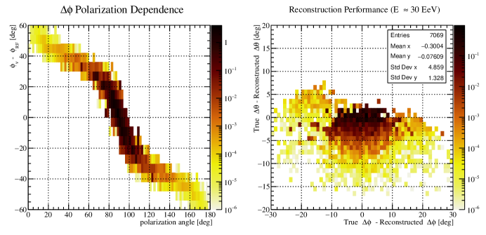
Figure 4: Left: The relationship between the reconstructed radio emission azimuth and the true neutrino direction as a function of reconstructed polarization angle for a diffuse neutrino flux. The reconstructed polarization angle is one component of the polynomial regression used for the fast approximate reconstruction. Right: The accuracy of the reconstruction for $\Delta\phi$ and $\Delta\theta$ for neutrinos at 30 EeV. Note that the color axes, which represent the relative number of weighted neutrinos, are logarithmic. The majority of poorly-reconstructed events have very low weights.

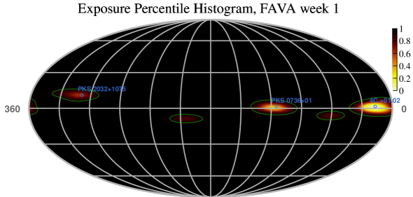
Figure 5: An example time slice of an exposure percentile histogram, in this case for the first week of FAVA-detected flaring blazars, which contains multiple sources of varying exposure. The value at each point $(\alpha^{\prime},\delta^{\prime},t)$ is set to the fraction of the total exposure with exposure density higher than the exposure density of the bin, so that lower values represent regions of relatively greater exposure. A cut in $\mathcal{D}$ defines the region in $(\alpha^{\prime},\delta^{\prime},t)$ with value smaller than the cut value, preferentially selecting regions with the greatest exposure density. The sources corresponding to the three highest-exposure regions are labeled, although note that in general there may be a systematic offset between the proxy sky position and the actual source coordinates. The green contours correspond to $\mathcal{D}=0.96$.

It remains to convert our per-event proxy sky position, $(\alpha^{\prime},\delta^{\prime})$, to a single source distance parameter to cut on. To avoid any assumptions about the shape or modality of the distribution, we use a simulation-driven approach to define $\mathcal{D}$. For each source class, we run a dedicated set of simulations with the appropriate neutrino directions and spectra, process the simulated events, and run the estimator regression. We then produce a three-dimensional exposure histogram with axes of reconstructed $\alpha^{\prime}$, $\delta^{\prime}$, and event time. For a steady source class, the time axis is extraneous and may be ignored. In the case of discrete source turn-on and turn-off times, it is convenient to choose the time bins to align with transitions.

The value of each exposure histogram bin can be interpreted as the relative exposure (exposure density) from this source class for events at that reconstructed time and estimated direction. We seek to define a parameter that smoothly selects the highest exposure density regions. To do this, the exposure histogram is converted to an exposure percentile histogram, where each bin’s value is set to the fraction of the total neutrino exposure with exposure density greater than the exposure of the bin (Figure  5). This results in a histogram where the bins with the highest exposure to the source class have values closer to 0 and bins with poor or no exposure have a values close to 1. We finally define $\mathcal{D}$ for an event and source class as the value of a source class’s exposure percentile histogram for its $\alpha^{\prime}$, $\delta^{\prime}$ and event time. This definition has the convenient property that setting the cut on $\mathcal{D}$ to $d\in[0,1]$ selects the highest exposure density region with an efficiency of approximately $d$.

Because it is time-consuming to generate enough simulated events to smoothly fill a exposure histogram at fine resolution, we actually start with a relatively coarsely binned $\alpha^{\prime}$ and $\delta^{\prime}$ axes and use a Gaussian kernel density estimator in each time slice to approximate a higher-resolution map. The kernel density estimator scale parameters are tuned so that the distribution of $\mathcal{D}$ for members of the source class is roughly uniform. Deviations from uniformity are not very concerning as long as efficiency varies smoothly with a cut on $\mathcal{D}$, so that the parameter can be effectively scanned. To reduce bias, disjoint sets of simulated data are used to create the exposure percentile histogram and for cut optimization, described next.

3.3 Cut Optimization

For each source class, we seek to set optimal cuts in a blind way on the $\mathcal{F}$ (the signal-likeness parameter), $\mathcal{O}$ (the spatial isolation parameter), and $\mathcal{D}$ (the source class distance parameter). We scan in these parameters to optimize expected sensitivity, using:

$$\rm{sens.}\propto\left<\frac{FC_{90}\left(Pois\left(\mu_{BG}\right),\mu_{BG}\right)}{\epsilon}\right>,$$ (3.3)

where $\mu_{BG}$ is the background estimate over the entire flight for a given set of cuts, $\epsilon$ is the expected analysis efficiency for a given set of cuts (the fraction of events that trigger ANITA that also pass analysis cuts), Pois is the Poisson distribution and FC₉₀(sig,bg) is the 90% Feldman-Cousins upper limit factor [30] for a given number of signal events and background events. As both $\mu_{bg}$ and $\epsilon$ have uncertainties, we calculate the expectation value in a semi-Bayesian way  [31] by integrating over their posterior distribution.

The estimate for analysis efficiency for a given set of cuts can be estimated from simulation by applying the cuts to simulated data. A Gaussian systematic error of 10% on the analysis efficiency is assumed, as derived in the diffuse analysis from calibration pulser data.

To estimate the background as a function of cut values, we use a data-driven on-off [32] approach based on time shuffling. For each event passing a trial $\mathcal{F}$ and $\mathcal{O}$, we create 100 off-time pseudoevents by shifting the event time by a random offset in either direction between 1.5 hours and 22.5 hours. These bounds are chosen to guarantee a significantly different sky position while preserving some time locality. We consider the pseudo-events an off-time sideband approximately seven times larger in phase space than the “on-time” signal region. We count the number of psuedoevents that pass the cut on $\mathcal{D}$ and the posterior on the background estimate is then conservatively taken to be the Poisson posterior using a uniform prior for a sideband seven times larger:

$$p(\mu_{BG})=\Gamma(7N_{pass}/100+1,1/7).$$ (3.4)

A different choice of prior (e.g. Jeffreys) would reduce the background estimate at the cost of some non-conservative coverage. This method is limited by the statistics of the sideband; as soon as the cuts are made so stringent that $N_{pass}$ is always zero, the background estimate will take a minimal value of ($0.10^{+0.16}_{-0.07}$), no matter how much more the cuts are tightened. Consideration of the efficiency in the sensitivity will typically shift the optimization to the boundary, somewhat alleviating this problem. An alternative would require a different strategy such as imposing a background model, which is difficult for the time-varying anthropogenic backgrounds faced by ANITA.

Using this methodology, we can perform a three-dimensional scan over reasonable parameters of $\mathcal{F}$, $-\log_{10}\mathcal{O}$, and $\mathcal{D}$ to choose cuts that optimize our sensitivity metric for any particular source class. Finally, as in the diffuse search, we only select events that are more impulsive in vertical polarization (VPol) than horizontal polarization (HPol) to avoid selecting air shower events.

4 Sources considered

Having developed a methodology to optimize cuts for a source class, we now turn our attention to potentially interesting sources for ANITA-III. Sources of the same type are pooled together into a single source class in order to reduce the global trials factor. This requires some model dependence in choosing the analysis cuts, but once cuts are chosen, model-independent limits may be placed on each source within the class. These limits may not be optimal for any given model other than the one used to set cuts, but we make an attempt to adopt a “least-common denominator” set of cuts to minimize the model-dependence.

Each search is optimized and performed independently, but the significance of any particular search’s result must be interpreted in the context of the number of searches performed. We considered optimizing for a global 90% significance (which is roughly equivalent to setting a higher optimized significance in each search, if they are weighted equally), but found that this did not strongly affect where the optimized cuts are placed, and we did not want to restrict the possibility of any additional future searches. It is also possible for a given event to be considered a candidate by multiple searches. The considered objects are tabulated in Table 1 and the result of each optimization is shown in Table 2.

Objects Considered Object Search Coordinates Times Considered (UTC) TXS 0506+056 TXS 0506+056 $\alpha=77.4^{\circ}$, $\delta=5.7^{\circ}$ Full Flight NGC 1068 NGC 1068 $\alpha=40.7^{\circ}$, $\delta=-0.0^{\circ}$ Full Flight 3C 454.3 Flaring Blazar $\alpha=344^{\circ},\delta=16.1^{\circ}$ 2014-12-15-15:43:38Z + 1 week 4C +01.02 Flaring Blazar $\alpha=17^{\circ},\delta=1.6^{\circ}$ 2014-12-15-15:43:38Z + 4 weeks * B3 1343+451 Flaring Blazar $\alpha=206^{\circ},\delta=44.8^{\circ}$ 2015-01-05-15:43:38Z + 1 weeks CTA 102 Flaring Blazar $\alpha=331^{\circ},\delta=11.7^{\circ}$ 2014-12-22-15:43:38Z + 3 weeks MG1 J221916+1806 Flaring Blazar $\alpha=335^{\circ},\delta=18.0^{\circ}$ 2014-12-15-15:43:38Z + 2 weeks * PKS 0402-362 Flaring Blazar $\alpha=61^{\circ},\delta=-36.0^{\circ}$ 2014-12-15-15:43:38Z + 4 weeks PKS 0502+049 Flaring Blazar $\alpha=76^{\circ},\delta=5.0^{\circ}$ 2014-12-22-15:43:38Z + 3 weeks PKS 0736+01 Flaring Blazar $\alpha=115^{\circ},\delta=1.5^{\circ}$ 2014-12-15-15:43:38Z + 2 weeks PKS 1441+25 Flaring Blazar $\alpha=221^{\circ},\delta=25.0^{\circ}$ 2014-12-15-15:43:38Z + 4 weeks PKS 1717+177 Flaring Blazar $\alpha=260^{\circ},\delta=17.7^{\circ}$ 2014-12-22-15:43:38Z + 2 weeks * PKS 1830-211 Flaring Blazar $\alpha=278^{\circ},\delta=-21.1^{\circ}$ 2015-01-05-15:43:38Z + 1 weeks PKS 2032+1075 Flaring Blazar $\alpha=309^{\circ},\delta=10.9^{\circ}$ 2014-12-15-15:43:38Z + 1 weeks * PKS 2052-47 Flaring Blazar $\alpha=314^{\circ},\delta=-47.3^{\circ}$ 2014-12-22-15:43:38Z + 2 weeks * PKS 2142-75 Flaring Blazar $\alpha=327^{\circ},\delta=-75.7^{\circ}$ 2014-12-15-15:43:38Z + 1 weeks PKS B1319-093 Flaring Blazar $\alpha=200^{\circ},\delta=-9.3^{\circ}$ 2014-12-15-15:43:38Z + 1 weeks * PMN J2141-6411 Flaring Blazar $\alpha=325^{\circ},\delta=-64.2^{\circ}$ 2014-12-29-15:43:38Z + 1 weeks RGB J2243+203 Flaring Blazar $\alpha=341^{\circ},\delta=20.3^{\circ}$ 2014-12-15-15:43:38Z + 2 weeks * S4 +1144+40 Flaring Blazar $\alpha=177^{\circ},\delta=40^{\circ}$ 2014-12-22-15:43:38Z + 1 weeks * S5 +1217+71 Flaring Blazar $\alpha=185^{\circ},\delta=71.1^{\circ}$ 2014-12-15-15:43:38Z + 2 weeks TXS +1100+122 Flaring Blazar $\alpha=166^{\circ},\delta=12.0^{\circ}$ 2014-12-29-15:43:38Z + 2 weeks GRB 141221A GRB $\alpha=198.3^{\circ},\delta=8.2^{\circ}$ 2014-12-21-08:07:02Z ${}_{\mathrm{-5min}}^{\mathrm{+1day}}$ * GRB 141223240 GRB $\alpha=147.4^{\circ},\delta=-20.7^{\circ}$ 2014-12-23-05:45:34Z ${}_{\mathrm{-5min}}^{\mathrm{+1day}}$ GRB 141226880 GRB $\alpha=163.9^{\circ},\delta=28.4^{\circ}$ 2014-12-26-21:07:24Z ${}_{\mathrm{-5min}}^{\mathrm{+1day}}$ GRB 141229911 GRB $\alpha=170.1^{\circ},\delta=23.1^{\circ}$ 2014-12-29-21:51:39Z ${}_{\mathrm{-5min}}^{\mathrm{+1day}}$ * GRB 141229A GRB $\alpha=72.4^{\circ},\delta=-19.2^{\circ}$ 2014-12-29-11:48:59 ${}_{\mathrm{-5min}}^{\mathrm{+1day}}$ GRB 141230834 GRB $\alpha=181.5^{\circ},\delta=11.6^{\circ}$ 2014-12-30-20:00:25Z ${}_{\mathrm{-5min}}^{\mathrm{+1day}}$ GRB 141230A GRB $\alpha=57.0^{\circ},\delta=1.6^{\circ}$ 2014-12-30-03:24:22Z ${}_{\mathrm{-5min}}^{\mathrm{+1day}}$ GRB 150101B GRB $\alpha=188.0^{\circ},\delta=-10.9^{\circ}$ 2015-01-01-15:23:00Z ${}_{\mathrm{-5min}}^{\mathrm{+1day}}$ GRB 150105A GRB $\alpha=124.3^{\circ},\delta=-14.8^{\circ}$ 2015-01-05-06:10:00Z ${}_{\mathrm{-5min}}^{\mathrm{+1day}}$ GRB 150106921 GRB $\alpha=40.8^{\circ},\delta=0.3^{\circ}$ 2015-01-06-22:05:53 ${}_{\mathrm{-5min}}^{\mathrm{+1day}}$ * SN 2014dz SN $\alpha=52.1^{\circ},\delta=38.0^{\circ}$ 2014-12-10-00:00:00Z + 2 weeks SN 2014dy SN $\alpha=42.2^{\circ},\delta=-0.8^{\circ}$ 2014-12-10-00:00:00Z + 2 weeks * SN 2015A SN $\alpha=145.3^{\circ},\delta=35.9^{\circ}$ 2015-01-02-00:00:00Z + 2 weeks SN 2015B SN $\alpha=193.6^{\circ},\delta=-12.6^{\circ}$ 2014-12-21-00:00:00Z + 2 weeks SN 2015D SN $\alpha=198.2^{\circ},\delta=12.6^{\circ}$ 2015-01-06-00:00:00Z + 2 weeks SN 2015E SN $\alpha=48.4^{\circ},\delta=0.3^{\circ}$ 2014-12-31-00:00:00Z + 2 weeks SN 2015W SN $\alpha=104.4^{\circ},\delta=13.6^{\circ}$ 2015-01-02-00:00:00Z + 2 weeks

Table 1: All objects considered in this search, along with coordinates and times the source is assumed to be turned on. ANITA-III launched Dec 18, 2014 and was terminated Jan 9, 2015. Objects with asterisks were included in the search but resulted in no passing simulated events. The times for the flaring blazar search are one-week time scales based on the Fermi telescope’s elapsed mission time, hence the offset of 15:43:38 for each start time.

Optimized cut values
Search $\mathcal{F}$ $-\log_{10}\mathcal{O}$ $\mathcal{D}$ exp. $\epsilon$ exp. backg. TXS 0506+056 $\geq$ 1.7 $\geq$ 0.9 $\leq$ 0.99 91.7% $0.10^{+0.16}_{-0.07}$ NGC 1068 $\geq$ 2.8 $\geq$ 0.5 $\leq$ 0.99 93.9% $0.10^{+0.16}_{-0.07}$ FAVA blazars $\geq$ 2.3 $\geq$ 0.9 $\leq$ 0.96 82.2% $0.30^{+0.25}_{-0.16}$ GRBs $\geq$ 1.7 $\geq$ 0.1 $\leq$ 0.96 92.7% $0.10^{+0.16}_{-0.07}$ SN $\geq$ 2.3 $\geq$ 0.9 $\leq$ 0.99 93.0% 0$.23^{+0.22}_{-0.13}$

Table 2: The optimized efficiency and background for each search performed for ANITA-III. The quoted efficiency is calculated for the model used to optimize the cuts and has an estimated uncertainty of order 10%. The background is model-independent. The 16%, 50% and 84% quantiles of the posterior distribution are used to determine the central value and errors quoted.

4.1 TXS 0506+056

The TXS 0506+056  blazar has been identified by IceCube as a potential source of astrophysical neutrinos. This association is due to a gamma-ray flare in spatial and temporal coincidence with a September 22, 2017 likely astrophysical neutrino candidate that triggered a multi-messenger alert [13]. Afterwards, archival data suggested an excess of neutrinos from the direction of TXS 0506+056 in a several-month window around December 2014 [14], albeit without any gamma-ray activity in the blazar [33]. The ANITA-III flight coincided temporally with this earlier neutrino “burst” and TXS 0506+056, at a declination of 5.6 degrees, is within ANITA-III’s sensitive field-of-view, motivating a dedicated search.

IceCube has measured a spectral index for the neutrino burst of $\gamma=2.1\pm{0.2}$. To optimize cuts for the ANITA-III search, we simulate neutrinos from the direction of TXS 0506+056 with $\gamma=2$, which is compatible with the IceCube measurement and somewhat preferred theoretically. The optimization results in an estimated analysis efficiency to an $E^{-2}$ flux of 91.7% with a background estimate of $0.10^{+0.16}_{-0.07}$, which is the minimal background estimate calculable with the method employed (i.e. zero passing sideband events).

4.2 NGC 1068

IceCube has identified NGC 1068 as a potential neutrino point source [15] at the 2.9$\sigma$ level. IceCube does not report any temporal information for NGC 1068, and the best-fit spectral index (3.2) from IceCube would make detection by ANITA-III unlikely. However, as it is one of just two objects within ANITA’s field of view that has been identified as a potential high-energy neutrino source at this significance level, a search is performed.

As the best-fit spectral index of $\gamma=3.2$ would make detection by ANITA virtually impossible, and moreover, there is no guarantee that a source must have consistent spectral index over many orders of magnitude of energy, we set cuts by simulating neutrinos from NGC 1068 with $\gamma=2$, resulting in an estimated analysis efficiency of 93.9% and a background of $0.10^{+0.16}_{-0.07}$ (the minimal allowed).

4.3 Flaring Blazars

Motivated in part by the apparent TXS 0506+056 flare coincidence, we consider blazars within the field of view of ANITA-III that are flaring in GeV gamma-rays as potential UHE neutrino sources. FSRQs in particular have been suggested as particularly-efficient neutrino sources above 1 EeV [16, 17, 18], although we consider all classes of blazars in this search. We use the Fermi Large Aperture Telescope’s All-sky Variability Analysis (FAVA) [24] to select flaring objects labeled as blazars by 3FGL [34] during the ANITA-III flight. FAVA identifies flaring candidates on a one-week cadence, during which we assume the neutrino flux is constant.

To set cuts, we weight neutrino flux from each blazar equally. While weighting by gamma-ray flux or luminosity distance are also reasonable, equal weighting is the least model-dependent, making it less likely to miss any interesting source. As before, we assume $\gamma=2$. The result of the optimization is an analysis efficiency estimate of 82.8% and an estimated background of $0.30^{+0.25}_{-0.16}$.

4.4 GRBs

GRBs, the brightest known transient events in the universe, have long been considered a potential source of UHE neutrinos [19, 20, 21, 22, 23]. ANITA is most likely most sensitive to the GRB afterglow neutrino flux, which is expected to have $\gamma=3/2$ up to some maximum energy (model-dependent, but typically order EeV).

We select GRBs from the IceCube GRBWeb catalog [35], which itself combines data from several sources [36, 37]. To optimize cuts, we chose to adopt a $\gamma=3/2$ spectrum, typical of afterglow models, up to 10 EeV for each GRB, starting five minutes before the GRB and extending 24 hours after. While most models would not predict neutrinos up to 10 EeV for most GRBs, this choice is inclusive and will avoid missing any potential signals. This time window would also tend to accept prompt and precursor neutrinos. The period of 24 hours is chosen as a compromise between too short a window, which might reject some of the most energetic afterglow neutrinos, and too long a window, which increases the possibility of chance coincidence. For the purpose of cut optimization, the relative normalization of each source’s flux was assumed to be proportional to the GRB fluence as measured by the Fermi Gamma-ray Burst Monitor, using a reasonable typical value if it was not available. Only GRBs with a declination within 30 degrees of the equator are considered. The cut optimization indicates an estimated analysis efficiency of 92.7% and the minimal possible background estimate of $0.10^{+0.16}_{-0.07}$.

4.5 Supernovae

Phenomena related to supernovae (SN) have been predicted to produce UHE neutrinos, especially in cases such as Hypernovae, magnetar-driven SN, transrelativistic SN, or tidal ignition of white dwarfs [38, 39, 40, 41, 42, 43]. Despite the lack of a clear model that might produce an observable signal in ANITA, their transient nature makes them amenable to a source search. Furthermore, the upward-air shower candidate in ANITA-III was spatially coincident with Supernova 2014dz [44], which likely occurred only several days before, further motivating a search in the Askaryan channel.

Due to a lack of clear model guidance for setting cuts, we select $\gamma=2$ and a two-week period after the estimated explosion date of the supernova, which is generally computed using spectral properties of the light curve at discovery. We select SN from the CBAT catalog [45] and do not distinguish between supernova types. Tidal disruption events (TDEs) were also considered, but none were catalogued near the time of the ANITA-III flight [46]. Optimization of cuts results in an estimated analysis efficiency of 93.0% on a background of $0.22^{+0.22}_{-0.13}$.

5 Results and Discussion

After applying the optimized cuts to each search using the procedure described above, all searches were null except for the SN search, which identified event 83134914 (Figure 6, left) as potentially associated with SN 2015D ($\mathcal{D}=0.67$). This is consistent with the background estimate for the search ($p=0.21$), even before accounting for the number of searches performed.

Due to a bookkeeping error in background estimation, initially a looser set of optimized cuts were computed and erroneously applied, which resulted in two additional passing events, 21318591 and 58125945 (Figure 6 center and right). As this initial unblinding did not follow the procedure prescribed ahead of time and these subthreshold events do not pass the final, corrected cuts, we do not consider them part of the result, though we briefly comment on them. All three events are summarized in Table 3.

Details about identified events

	Candidate	Subthreshold	Subthreshold
	Ev. 83134914	Ev. 21318591	Ev. 58125945
Time	2015-01-08-19:04:24.237	2014-12-22-04:30:24Z	2015-01-01-08:17:14.615Z
Payload Pos.	70.3S, 90.1E, 33.6 km	80.2S, 82.0E, 36.6 km	76.2S, 108.6W, 34.6 km
Est. Ice Pos..	68.6S, 98.2ES	81.8S, 94.7E	74.4S, 100.3W
Proxy Sky Pos.	$\alpha^{\prime}=206^{\circ}$,$\delta^{\prime}=13.6^{\circ}$	$\alpha^{\prime}=38^{\circ}$, $\delta^{\prime}=-3.1^{\circ}$	$\alpha^{\prime}=164^{\circ},\delta^{\prime}=11.7^{\circ}$
Potential	SN 2014 D ($\mathcal{D}=0.67$)	4C +01.02 ($\mathcal{D}=0.955)$	TXS 1100+122 ($\mathcal{D}=0.003)$
Associations		NGC 1068 ($\mathcal{D}$ =0.64)
		SN 2014dy ($\mathcal{D}$ =0.78)
$\mathcal{F}$	3.03	2.28	3.06
$-\log_{10}\mathcal{O}$	$\sim\infty$	0.41	0.68

Table 3: Details about the candidate event and subthreshold events that were associated with searches. Event 83134914 was identified by the SN search as potentially associated with SN 2015D. This event was previously identified in the diffuse ANITA-III analysis. The other two events were subthreshold and revealed due to an error in the initial unblinding, but are included here for completeness.

5.1 Candidate Event 83139414

The sole candidate event this search, event 83134914, was previously identified in the ANITA-III diffuse search [6] as being neutrino-like and extremely isolated. In this search, it was found to be potentially associated with SN 2015D [47], which was discovered approximately 10 days after this event and believed to be around two weeks old at the time of discovery.

We note that that the proxy position for this event in this search ($\alpha^{\prime}=206$ , $\delta^{\prime}=13.9$) differs substantially from what was reported in the diffuse search ($\alpha=171\pm 5$ , $\delta=16.3\pm 1$), a position which would have failed the association cut here. The previous estimate was performed by dedicated simulations with the payload at that position, rather than the approximate method used in this paper, which is designed to reduce dispersion rather than produce a bias-free position estimator. Moreover, the handling of polarization in the simulation software has also been improved since the previous estimate was made, adding another potential source of discrepancy. For the purpose of this search, the event is associated even if the localization proxy differs from the previous estimate.

This event points to isolated deep ice, very far from any known anthropogenic activity and would have passed a much more stringent isolation cut. If, hypothetically, the selection cuts were set to barely accommodate this event, the background estimate for the supernova search would be the minimal possible with the method used ($0.10^{+0.16}_{-0.07}$), which would modify the pre-trial significance of this event to $p=0.13$. This is not enough to be interesting by itself, but is perhaps more interesting in combination with the potential association of the apparently upward air-shower in ANITA-III with an SN, which had $p=0.0017-0.023$, depending on the prior used for the time dependence [44, Supplemental Material].

To get a feeling for the false association rate, should 83134914 be an anthropogenic event, we consider the sideband of VPol-identified events with $\mathcal{F}\in[1,2]$, $-\log_{10}\mathcal{O}\in[-1,1]$. Of these 173 sideband events, 4 (2.3%) would have passed the SN association cut value and just one event has an association as good as the candidate. 22 events (12.7%) in this sideband pass the association cut for any of the five source classes.

It is possible that 83134914 is a UHE neutrino event and not some anthropogenic background, but is associated with a SN direction by chance. By simulating a diffuse cosmogenic neutrino flux we find 10% of simulated diffuse neutrinos would be considered SN-associated in this search and 24% would be considered associated with any of the source classes at each search’s cut level.

A subthreshold search in the direction of SN 2015D down to $\mathcal{F}=0$ and $-\log_{10}\mathcal{O}=0$ was performed, yielding one additional event. This event was isolated but was only marginally-associated with SN2014D and upon further inspection, is potentially residual radio interference from satellites.

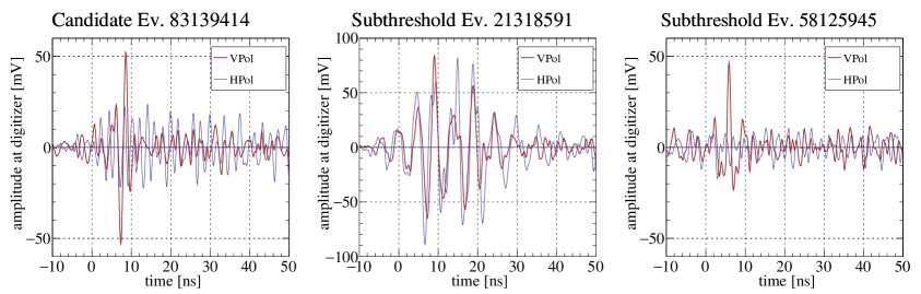
Figure 6: The candidate event (left) and two subthreshold events identified in this analysis. These waveforms represent a coherent sum based on the estimated radio direction and with the group delay from filters and antennas removed.

5.2 Subthreshold Events 21318591 and 58125945

The cuts associated with the initial unblinding of the searches erroneously underestimated the background estimate due to a software bug involving an inconsistency in histogram binning. This resulted in less stringent optimized cuts that selected events 21318591 and 58125945 as candidates. We stress that these events do not pass the final cuts after correctly applying the optimization procedure and are not considered a part of the results. However, these events would represent the result of a valid—albeit less sensitive—search with slightly higher efficiency and a significantly higher (by a factor of 2-3) background estimate. We briefly discuss these accidentally unveiled events here for completeness and transparency.

Event 21318591 was initially considered a candidate in multiple searches (NGC 1068, SN, Flaring Blazars), although, with $\mathcal{F}=2.3$ and $-\log_{10}\mathcal{O}=0.4$, it fails the corrected cuts for all searches, is less impulsive than a typical neutrino event, has an unlikely polarization for a neutrino, and the nearby events have similar shapes.

Event 58125945 was initially identified as associated with flaring blazar TXS 1100+122. With $-\log_{10}\mathcal{O}=0.7$, it fails the corrected isolation cut of 0.9 for the FAVA search, although it is the closest event to passing. This event is impulsive and virtually purely VPol, but points to the Pine Island Glacier, a part of the continent with relatively low likelihood to produce detectable Askaryan neutrino events due to high temperature and relatively low ice thickness. While fairly isolated, the nearest neighbors, which form a cluster with each other, look broadly similar to this event. Moreover, the British Antarctic Survey was conducting radar and drilling studies in Pine Island Glacier during the 2014-2015 season [48]. Due to a storm on January 1, there was no significant activity at the time of the event [49], but a storm also admits the possibility of triboelectric emission [50]. While this event is clearly consistent with background and did not pass the corrected cut, we note that TXS 1100+122 has been suggested as a potentially interesting neutrino source [51], on the basis of TXS 1100+122 being compatible in position with IceCube alert event (IC-200109A [52]) and possessing a compact radio emission core, a feature suggested as possibly being associated with neutrino emission [53].

5.3 Limits

As we do not find any significant associations, we proceed to set upper limits on fluence during the ANITA-III flight from each source. Model-independent limits on fluence at a given energy $\Phi(E)$ are given by

$$u.l.(E^{2}\Phi(E))=\left<\frac{FC_{90}(n_{obs},\mu_{bg})\cdot E}{\epsilon A_{eff}(E)\cdot\Delta}\right>,$$ (5.1)

where $\Delta$ is a factor compensating for the use of discrete energies, while the flux and acceptance both evolve continuously. ANITA cosmogenic searches have typically used $\Delta=4$ [25], based on studies showing that this is a reasonable choice for a variety of models [54]. We maintain this convention here for consistency, but note that other experiments use different conventions.

Setting limits on objects within multi-member source classes requires additional consideration in the handling of the background estimate, as this estimate applies to the entire class, rather than individual objects. However, the true limit is be bounded by ascribing zero background to a source and ascribing the total background of the source class to a source, and this difference is small ($\mathcal{O}(10\%)$) in all cases here. We choose to ascribe zero background as that results in more conservative (higher) limits. Upper limits for each source are shown in Figure 7. Some sources are omitted due to a paucity of simulated triggered events or low analysis efficiency.

In addition to model-independent energy-dependent limits, we show integrated $\gamma=2$ limits for AGN-like and SN searches, where the upper limit on normalization for a $\Phi(E)=\Phi{{}_{0}}(E^{-2})$ is calculated using:

$$u.l.(\Phi_{0})=\left<\frac{FC_{90}(n_{obs},\mu_{bg})\cdot\phi_{0}}{\left<\epsilon\cdot A_{eff}(E)\right>|_{\phi(E)}}\right>,$$ (5.2)

where $A_{eff}$ and $\epsilon$ are averages over the unity-normalized flux $\phi(E)=\phi_{0}E^{-2}$, with $\phi_{0}=1.00$ EeV for the energy range considered.

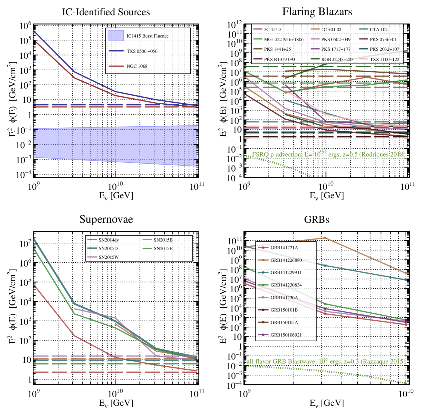
Figure 7: ANITA-III limits on neutrino fluence for all objects considered in these searches. The top-left panel shows fluence limits on TXS 0506+056 and NGC 1068, along with the extrapolated time-scaled fluence from the 2014-2015 apparent IceCube neutrino burst in the direction of TXS 0506+056. The top right shows fluence limits flaring blazars that result in triggered simulated events (points are not shown at energies with no simulated passing events). Some blazars (e.g RGB J2243+203) suffer from poor geometry. We include an optimistic model for neutrinos from an FSRQ in a high-luminosity state, based on  [18]. The bottom left shows fluence limits on SN and the bottom right shows fluence limits on GRBs. For GRBs, we compare the limits to a model for neutrinos produced in the afterglows from a nearby, luminous GRB  [22]. Model-independent limits are shown with solid lines and integrated $E^{-2}$ limits are shown with dashed lines, where appropriate.

The measured fluence for the apparent 2014-2015 TXS 0506+056 neutrino flare from IceCube was $E^{2}\Phi(E)=(0.21^{+0.09}_{-0.07})~{}\mathrm{GeVcm}^{-2}(E/10^{5}\mathrm{GeV})^{2-2.1\pm 0.2}$ over a Gaussian window centered on 2014-12-14$\pm 14$ days with a width of $110^{+34}_{-24}$ days [14]. The ANITA-III flight time represents a fraction of 0.16 of this time window. This fluence band, scaled to the ANITA-III flight time, is projected onto the top-left panel of Figure 7. We also superimpose some relevant models for GRBs and flaring blazars.

6 Conclusion and Outlook

We find that there is no significant evidence for any source-associated neutrinos with ANITA-III, although the potential SN association of the ANITA-III diffuse analysis event is somewhat intriguing, especially in combination with previous results.

The methodology developed is shown to be capable of achieving higher efficiencies at lower backgrounds compared to a diffuse search. However, because the analysis efficiency of the ANITA-III diffuse search was already high ($>$80%), there is relatively little room for neutrinos that could have triggered ANITA-III but not have passed analysis cuts employed in the diffuse search. As such, a null result is not surprising. Still, using this methodology we are able to set limits on individual sources with ANITA, which can not be done coherently in the diffuse search. A similar search is in progress for the more recent and more sensitive ANITA-IV payload, although that also had a high diffuse analysis efficiency.

For similar experiments where the achieved diffuse analysis efficiency at an acceptable background level is not as high, the methodology described here can be more impactful, as there is additional phase space for discovery currently not accessible to diffuse searches. For example, a significant gap currently exists between diffuse analysis and trigger efficiency in the Askaryan Radio Array (ARA) experiment [55]. Employing an adaptation of the method described here therefore has the potential to discover new candidates within the ARA dataset

Similarly, it follows that it is advantageous for future UHE radio neutrino experiments to reduce trigger thresholds below expected achievable analysis thresholds for diffuse searches. A reduced trigger threshold could not be achieved in ANITA-III or ANITA-IV as the acquisition system could not handle the corresponding increased data rate. Future UHE neutrino detectors using the Askaryan method such as PUEO [56], RNO-G [57], or the radio extension of IceCube Gen2 [58] will use improved trigger techniques capable of substantially reducing the achievable trigger thresholds while maintaining lower rates. If the threshold is chosen to be low enough, then the techniques developed here can potentially unveil candidate events not discoverable in a diffuse search.

The method outlined here suffers from an inability to reduce background below some level, due to the use of a sideband for background estimation. Finding additional handles on background could potentially further reduce background and help improve sensitivity. This may be accomplished through improved modeling of anthropogenic backgrounds (easier in the case of fixed-position detectors than balloon payloads) or through the use of sidebands with relatively more phase space (for example, by improving angular reconstruction or introducing additional variables). With the minimal background estimate achievable in this analysis, four events are necessary for $>3\sigma$ evidence and eight events would be required for $>5\sigma$ discovery, before accounting for trials factors. Doubling the relative size of the sideband, for example, would reduce the number of events required to exceed each significance threshold by one. We note that the planned PUEO mission is projected to be more than an order of magnitude more sensitive than ANITA-III, implying that a transient fluence producing one event in ANITA-III would likely yield a statistically-significant excess in PUEO.

References

- [1] ANITA collaboration, The Antarctic Impulsive Transient Antenna ultra-high energy neutrino detector: Design, performance, and sensitivity for the 2006-2007 balloon flight, Astropart. Phys. 32 (2009) 10 [0812.1920].
- [2] G. Askaryan, Excess negative charge of an Electron-photon shower and its coherent radio emission, Sov. Phys. JETP 14 (2) (1962) 441.
- [3] ANITA collaboration, Observations of the Askaryan effect in ice, Phys. Rev. Lett. 99 (2007) 171101 [hep-ex/0611008].
- [4] ANITA collaboration, New Limits on the ultra-high energy cosmic neutrino flux from the ANITA experiment, Phys. Rev. Lett. 103 (2009) 051103 [0812.2715].
- [5] ANITA collaboration, Observational constraints on the ultra-high energy cosmic neutrino flux from the second flight of the ANITA experiment, Phys. Rev. D 82 (2010) 022004.
- [6] ANITA collaboration, Constraints on the diffuse high-energy neutrino flux from the third flight of ANITA, Phys. Rev. D 98 (2018) 022001 [1803.02719].
- [7] ANITA collaboration, Constraints on the ultrahigh-energy cosmic neutrino flux from the fourth flight of ANITA, Phys. Rev. D 99 (2019) 122001 [1902.04005].
- [8] ANITA collaboration, The First Limits on the Ultra-high Energy Neutrino Fluence from Gamma-ray Bursts, Astrophys. J. 736 (2011) 50 [1102.3206].
- [9] K. Greisen, End to the cosmic ray spectrum?, Phys. Rev. Lett. 16 (1966) 748.
- [10] G. Zatsepin and V. Kuzmin, Upper limit of the spectrum of cosmic rays, JETP Lett. 4 (1966) 78.
- [11] K. Kotera, D. Allard and A.V. Olinto, Cosmogenic neutrinos: parameter space and detectabilty from PeV to ZeV, J. Cosmol. Astropart. Phys. 10 (2010) 13 [1009.1382].
- [12] IceCube collaboration, Evidence for high-energy extraterrestrial neutrinos at the icecube detector, Science 342 (2013) [1311.5238].
- [13] IceCube, Fermi-LAT, MAGIC, AGILE, ASAS-SN, HAWC, H.E.S.S., INTEGRAL, Kanata, Kiso, Kapteyn, Liverpool Telescope, Subaru, Swift NuSTAR, VERITAS, VLA/17B-403 collaboration, Multimessenger observations of a flaring blazar coincident with high-energy neutrino IceCube-170922A, Science 361 (2018) eaat1378 [1807.08816].
- [14] IceCube collaboration, Neutrino emission from the direction of the blazar TXS 0506+056 prior to the IceCube-170922A alert, Science (2018) eaat2890 [1807.08794].
- [15] IceCube collaboration, Time-Integrated Neutrino Source Searches with 10 Years of IceCube Data, Phys. Rev. Lett. 124 (2020) 051103 [1910.08488].
- [16] C. Righi et al., EeV Astrophysical neutrinos from FSRQs?, 2003.08701.
- [17] X. Rodrigues et al., Blazar origin of the UHECRs and perspectives for the detection of astrophysical source neutrinos at EeV energies, 2003.08392.
- [18] X. Rodrigues et al., Neutrinos and ultra-high-energy cosmic-ray nuclei from blazars, The Astrophysical Journal 854 (2018) 54.
- [19] E. Waxman and J.N. Bahcall, Neutrino afterglow from gamma-ray bursts: -eV, Astrophys. J. 541 (2000) 707 [hep-ph/9909286].
- [20] K. Murase, High energy neutrino early afterglows gamma-ray bursts revisited, Phys. Rev. D76 (2007) 123001 [0707.1140].
- [21] E. Waxman and J.N. Bahcall, High-energy neutrinos from cosmological gamma-ray burst fireballs, Phys. Rev. Lett. 78 (1997) 2292 [astro-ph/9701231].
- [22] S. Razzaque and L. Yang, PeV-EeV neutrinos from GRB blast waves in IceCube and future neutrino telescopes, Phys. Rev. D 91 (2015) 043003 [1411.7491].
- [23] J.K. Thomas, R. Moharana and S. Razzaque, Ultrahigh energy neutrino afterglows of nearby long duration gamma-ray bursts, Phys. Rev. D 96 (2017) 103004 [1710.04024].
- [24] S. Abdollahi et al., The Second Catalog of Flaring Gamma-Ray Sources from the Fermi All-sky Variability Analysis, Astrophys. J. 846 (2017) 34 [1612.03165].
- [25] ANITA collaboration, The Simulation of the Sensitivity of the Antarctic Impulsive Transient Antenna (ANITA) to Askaryan Radiation from Cosmogenic Neutrinos Interacting in the Antarctic Ice, JINST 14 (2019) P08011 [1903.11043].
- [26] P. Fretwell et al., Bedmap2: improved ice bed, surface and thickness datasets for antarctica, Cryosphere 7 (2013) 375.
- [27] ANITA collaboration, Observation of ultrahigh-energy cosmic rays with the anita balloon-borne radio interferometer, Physical Review Letters 105 (2010) .
- [28] J. Alvarez-Muniz, A. Romero-Wolf and E. Zas, Practical and accurate calculations of Askaryan radiation, Phys. Rev. D 84 (2011) 103003 [1106.6283].
- [29] A. Hoecker et al., TMVA - Toolkit for Multivariate Data Analysis, PoS ACAT2007 (2007) 040 [physics/0703039].
- [30] G.J. Feldman and R.D. Cousins, A Unified approach to the classical statistical analysis of small signals, Phys. Rev. D 57 (1998) 3873 [physics/9711021].
- [31] R.D. Cousins and V.L. Highland, Incorporating systematic uncertainties into an upper limit, Nucl. Instrum. Meth. A 320 (1992) 331.
- [32] T.P. Li and Y.Q. Ma, Analysis methods for results in gamma-ray astronomy., Astrophys. J. 272 (1983) 317.
- [33] P. Padovani et al., Dissecting the region around IceCube-170922A: the blazar TXS 0506+056 as the first cosmic neutrino source, Monthly Notices of the Royal Astronomical Society 480 (2018) 192–203 [1807.04461].
- [34] Fermi-LAT collaboration, Fermi Large Area Telescope Third Source Catalog, Astrophys. J. Suppl. 218 (2015) 23 [1501.02003].
- [35] P. Coppin, GRBWeb, 2020. https://icecube.wisc.edu/~grbweb_public/.
- [36] A. Lien et al., The Third Swift Burst Alert Telescope Gamma-Ray Burst Catalog, Astrophys. J. 829 (2016) 7 [1606.01956].
- [37] A. von Kienlin et al., The fourth Fermi-GBM gamma-ray burst catalog: A decade of data, The Astrophysical Journal 893 (2020) 46 [2002.11460].
- [38] X.-Y. Wang, S. Razzaque, P. Meszaros and Z.-G. Dai, High-energy Cosmic Rays and Neutrinos from Semi-relativistic Hypernovae, Phys. Rev. D 76 (2007) 083009 [0705.0027].
- [39] B.T. Zhang and K. Murase, Ultrahigh-energy cosmic-ray nuclei and neutrinos from engine-driven supernovae, Phys. Rev. D 100 (2019) 103004 [1812.10289].
- [40] K. Murase, P. Meszaros and B. Zhang, Probing the birth of fast rotating magnetars through high-energy neutrinos, Phys. Rev. D 79 (2009) 103001 [0904.2509].
- [41] D. Biehl, D. Boncioli, C. Lunardini and W. Winter, Tidally disrupted stars as a possible origin of both cosmic rays and neutrinos at the highest energies, Sci. Rep. 8 (2018) 10828 [1711.03555].
- [42] R. Alves Batista and J. Silk, Ultrahigh-energy cosmic rays from tidally-ignited white dwarfs, Phys. Rev. D 96 (2017) 103003 [1702.06978].
- [43] K. Murase, New Prospects for Detecting High-Energy Neutrinos from Nearby Supernovae, Phys. Rev. D 97 (2018) 081301 [1705.04750].
- [44] ANITA collaboration, Observation of an unusual upward-going cosmic-ray-like event in the third flight of anita, Phys. Rev. Lett. 121 (2018) 161102.
- [45] CBAT, CBAT SN catalog, 2015.
- [46] J. Guillochon, Open TDE catalog, 2020. http://TDE.space.
- [47] Z.w. Jin et al., Supernova 2015D in NGC 5020 = Psn J13124116+1236018, Central Bureau Electronic Telegrams 4051 (2015) 1.
- [48] R. Mulvaney and A.M. Smith, Borehole derived pine island glacier mean annual temperatures, NERC Polar Data Centre (2017) .
- [49] R. Mulvaney. Private Communication, 2020.
- [50] ANITA collaboration, Experimental tests of sub-surface reflectors as an explanation for the ANITA anomalous events, 2009.13010.
- [51] Y.Y. Kovalev et al., Flat spectrum radio quasar TXS 1100+122 has a bright VLBI-compact core - as expected for neutrino candidate sources, The Astronomer’s Telegram 13397 (2020) 1.
- [52] IceCube collaboration, IceCube-200109A: IceCube observation of a high-energy neutrino candidate event, GRB Coordinates Network 26696 (2020) 1.
- [53] A. Plavin, Y. Kovalev, Y. Kovalev and S. Troitsky, Observational evidence for the origin of high-energy neutrinos in parsec-scale nuclei of radio-bright active galaxies, Astrophys. J. 894 (2020) 101 [2001.00930].
- [54] I. Kravchenko et al., RICE limits on the diffuse ultrahigh energy neutrino flux, Phys. Rev. D 73 (2006) 082002 [astro-ph/0601148].
- [55] ARA collaboration, Constraints on the diffuse flux of ultrahigh energy neutrinos from four years of askaryan radio array data in two stations, Phys. Rev. D 102 (2020) 043021 [1912.00987].
- [56] PUEO collaboration, The Payload for Ultrahigh Energy Observations (PUEO): A white paper, 2010.02892.
- [57] RNO-G collaboration, J. Aguilar et al., Design and sensitivity of the Radio Neutrino Observatory in Greenland RNO-G, 2020. Under preparation.
- [58] IceCube Gen2 collaboration, IceCube-Gen2: The Window to the Extreme Universe, 2008.04323.
- [59] F. Rademakers et al., root-project/root: v6.18/02, Aug., 2019. 10.5281/zenodo.3895860.
- [60] R. Brun and F. Rademakers, ROOT: An object oriented data analysis framework, Nucl. Instrum. Meth. A 389 (1997) 81.