Network Localization Based Planning for Autonomous Underwater Vehicles with Inter-Vehicle Ranging

Abstract

Localization between a swarm of AUVs can be entirely estimated through the use of range measurements between neighboring AUVs via a class of techniques commonly referred to as sensor network localization. However, the localization quality depends on network topology, with degenerate topologies, referred to as low-rigidity configurations, leading to ambiguous or highly uncertain localization results. This paper presents tools for rigidity-based analysis, planning, and control of a multi-AUV network which account for sensor noise and limited sensing range. We evaluate our long-term planning framework in several two-dimensional simulated environments and show we are able to generate paths in feasible time and guarantee a minimum network rigidity over the full course of the paths.

I INTRODUCTION

Multi-AUV swarms bear the promises of increased coverage, greater efficiency in ocean deployments, and improved ability to track spatially and temporally dynamic oceanographic phenomena. However, the lack of Global Navigation Satellite System (GNSS) and sparsity of salient features for navigation present substantial challenges in accurately localizing each AUV underwater, a required ability for real-world deployment. Additionally, severe communication constraints due to the underwater environment limit multi-AUV systems to techniques which require minimal communications. These combined challenges in localization and communication greatly limit the deployment of multi-AUV networks.

The simultaneous localization and mapping community has developed a large number of techniques which use observations of environmental features to allow for autonomous localization, but these techniques often extend poorly to the underwater domain due to a common sparsity of features to observe, large amount of error in observations made, and oftentimes a need for relatively large data transmissions [1]. Previous works [2] in single-AUV localization rely upon the use of costly inertial navigation systems which offer greatly reduced drift in dead-reckoned estimates. However, such systems can often cost hundreds of thousands of dollars, which becomes cost-prohibitive when scaling to multi-AUV swarms. Recent work [3] proposed one-way acoustic communications to perform formation control in which ‘followers’ keep relative positioning to a ‘leader’. While this allows for localization and reduced communication, this limits configurations to predetermined geometries and relies on functionality of the ‘leader’.

Sensor network localization (SNL) is a promising set of localization techniques for multi-AUV networks which use inter-AUV range measurements to estimate relative position of network members [4]. Furthermore, knowing the absolute location of four network members, via GNSS or inertial navigation, is fully sufficient to fix the absolute coordinates of the entire network and provide absolute three dimensional localization of all others. This allows for complete localization using only range measurements and depending on the operational requirements can enable localization in which a small number of AUVs use GNSS fixes to maintain absolute localization for the entire network. Such an approach allows use of recently developed low-cost ranging technology [5] and absolves need for high-cost inertial navigation solutions or fixed acoustic beacons.

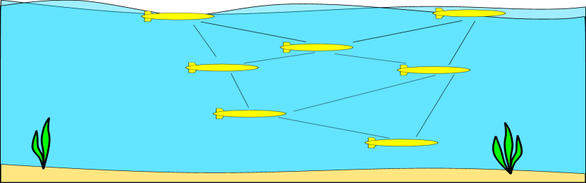
Figure 1: Example multi-AUV network. Edges between AUVs represent distance measurements between corresponding vehicles. Surfacing AUVs can use GNSS for absolute positioning, thus serving as reference positions for the entire swarm and allowing absolute localization of the entire swarm.

Many distributed and centralized SNL techniques have been developed to robustly perform localization in the presence of noisy range measurements [6, 7]. However, it is well known that the accuracy of SNL approaches depend on the topology of the network, with certain ’poor’ network configurations causing high localization error [8].

We consider the problem of generating paths to a set of goal locations for a multi-AUV network while ensuring that the network remains in configurations robust to noise. We use the rigidity eigenvalue [9] to measure the robustness of a configuration, which we term network rigidity. Previous work considering similar networks of robots [10] developed a linear algebraic representation of network rigidity and proposed gradient-based controls to maintain network rigidity. This work was extended by [9] in which the linear-algebraic representation of network rigidity was modified to consider an information theoretic interpretation of network rigidity and the use of potential-field planning was proposed. However, both of these approaches relied on the use of gradient-based controls to maneuver such multi-agent networks, which can cause highly inefficient paths to be generated and are inherently at risk of getting stuck in local-minima during planning and therefore prevented from reaching target locations.

To address these issues we formulate a prioritized path-planning framework [11] which leverages the underlying structure of network rigidity to more efficiently compute paths which enforce minimum network rigidity. To make our algorithm more robust to the possibility of a valid set of trajectories not being found, we make use of a conflict identifying mechanism which attempts to find trajectories which degrade the rigidity of the network. Though our approach differs from previous works in conflict-based multi-agent planning [12], there is similarity in that conflicts are used to aid planning. We evaluate our approach in simulation and show our framework successfully finds paths in reasonable time while maintaining minimum network rigidity.

II METHODS

We seek to develop a framework for scalable, rigidity constrained multi-AUV path-planning that allows for unambiguous and robust localization via SNL techniques. For simplicity, we constrain ourselves to a two-dimensional system, but note that extension to higher dimensions is straightforward.

II-A Network Rigidity

We quantify network rigidity based on the eigenvalues of a network’s derived Fisher information matrix (FIM). As in [9, 13], for a given network configuration under the assumption of Gaussian measurement noise we define the Fisher information matrix, $F=A^{T}A$ where $A\in\mathbb{R}^{m\times dn}$, $m$ is the number of measurements, $d$ the dimensionality of the system, and $n$ the number of nodes. The rows of $A$ correspond to measurements between network nodes (AUVs), with a single row per measurement. Defined below, $row_{m}$ denotes the row corresponding to measurement $m$ with standard deviation $\sigma$ between nodes $i$ and $j$. The value of $\alpha$ depends on whether the measurement model represents Gaussian additive or multiplicative noise.

It it proven that the inverse of the FIM is the lower bound on the variance of an unbiased estimator, commonly referred to as the Cramér-Rao Lower Bound (CRLB) [14]. Though the actual estimation variance relies on the estimation technique used and the CRLB cannot be achieved in many cases, this provides an information-theoretic limit for the uncertainty of an estimation technique. Importantly, this implies that in our specific case the eigenvalues of the FIM have an inverse relationship with the best possible localization uncertainty. That is, lower eigenvalues correspond to increased best-case uncertainty in localization results.

$$\Delta_{x} =x_{i}-x_{j}$$ (1)

$$\Delta_{y} =y_{i}-y_{j}$$ (2)

$$L =\sqrt{\Delta_{x}^{2}+\Delta_{y}^{2}}$$ (3)

$$\alpha =\begin{cases}1&\textit{Additive Noise}\\ 2&\textit{Multiplicative Noise}\\ \end{cases}$$ (4)

$$row_{m} =\dfrac{1}{\sigma L^{\alpha}}\begin{cases}\Delta_{x}&\textit{index}=2i\\ \Delta_{y}&\textit{index}=2i+1\\ -\Delta_{x}&\textit{index}=2j\\ -\Delta_{y}&\textit{index}=2j+1\\ 0&\textit{otherwise}\end{cases}$$ (5)

Because of the natural relationship between the eigenvalues of the FIM and the localization uncertainty, we use these eigenvalues as a heuristic measure for the localizability of a network configuration, or, as was previously introduced, the network rigidity. Similar to [9, 10], we define network rigidity for a given sensor network as the least nontrivial eigenvalue of $F$, where trivial eigenvalues are all zero and have been shown [10] to correspond to the degrees of freedom (DOF) of a the special Euclidean space the network occupies (e.g. two-dimensional space being 3-DOF). It has been theoretically shown that a non-zero network rigidity is required to find unique solutions to the range-only localization problem [4].

To heuristically control the localizability of a network we will enforce a minimum rigidity during the trajectory planning sequence, below which a network will be considered nonrigid and disallowed. This causes our proposed planning technique to perform a large number of eigenvalue computations. For this reason, it is important to note that it directly follows from the construction of $F=A^{T}A$ that $F$ is a positive semidefinite matrix, and thus has only real, non-negative eigenvalues. In practice we leverage this fact to use computational methods that are specially designed for Hermitian matrices, which positive semidefinite matrices are a subclass of, to reduce the time required to perform these eigenvalue computations.

II-B Path-Planning

From here our approach takes the form of priority-based multi-agent planning on a single graph. In our methodology planning on a graph is meant to indicate that all agents share a common graph in which nodes are locations, edges connect neighboring locations according to some set of predetermined rules, that the agents are only considered to occupy the nodes of the graph, and that the agents move through the world by moving along these edges between neighboring nodes [15]. Priority-based planning indicates that each agent individually performs planning on this graph in a predetermined sequence.

In the planning process we impose the constraint that no two agents can occupy the same location at the same time and that network rigidity must remain above a pre-specified minimum rigidity for all timesteps. In addition, we apply a heuristically driven technique which attempts to avoid low-rigidity configurations early in the planning sequence. This is to prevent going through the entire planning sequence when early in the planning sequence the already planned trajectories would likely result in low-rigidity configurations regardless of the subsequent trajectories

Though network rigidity is not guaranteed to monotonically increase as agents are added to the network, as a heuristic measure to avoid low-rigidity configurations early in the planning sequence we enforce that every agent must plan a path which stays entirely within the valid set, $V$, defined later in this section. This reduces the search space, reducing necessary computation at the cost of potentially rejecting valid full-network trajectories.

This framework was chosen to address several practical concerns in multi-agent planning. We look to avoid gradient-based methods due the previously mentioned issues of local minima, particularly as the number of AUVs increase and the potential fields used run the risk of growing complexity and increased number of local minima. Similarly, as the number of AUVs increase the dimensionality of the planning space increases. The use of priority planning reduces the dimension of the planning space from $(n\times d)$ to $d$.

Furthermore, planning on graphs allows the use of sampling based planning techniques, which have empirically found success in reducing the combinatorial cost of high-dimensional problems such as multi-agent planning. Importantly, the graph-based structure also allows for straightforward bookkeeping and recycling of certain computations as the planning process occurs; this is discussed in the remainder of this section.

To perform this bookkeeping and reduce unnecessary computation during planning we use multiple set-based representations of locations on the planning-graph, with there being distinct collections of these sets that correspond to each AUV and timestep. We will first describe the sets and how they are constructed and then explain how they are used to perform bookkeeping and eliminate unnecessary computation. As our planning technique is priority-based, sets for AUV $0$ are quickly computed upon construction of the planning graph. For all other AUVs, the sets for AUV $n$ are computed after planning by AUV $n-1$.

For the $ith$ AUV at time $t$ we denote the sets: reachable ($\mathbf{P_{i,t}}$), connected ($\mathbf{C_{i,t}}$), rigid ($\mathbf{R_{i,t}}$), and valid ($\mathbf{V_{i,t}}$). $\mathbf{C_{i,t}}$ is the set of all states which would be within sensing radius of AUVs $(0,1,...,i-1)$ at time $t$. $\mathbf{R_{i,t}}$ is the set of all states which AUV $i$ could occupy at time $t$ that would allow for AUVs $0,1,..,i$ to form a network that satisfies the minimum rigidity constraint. $\mathbf{P_{i,t}}$ is the set of all locations which are connected to a location in $\mathbf{V_{i,t-1}}$ for AUV $i$ at time $t$. $\mathbf{V_{i,t}}$ is the set of allowable states, which the AUVs are required to use for planning. We define $\mathbf{V_{i,t}}$ and note the relationship between $\mathbf{R_{i,t}}$ and $\mathbf{C_{i,t}}$ in Equations (6$-$7).

The purpose of these sets of graph locations is to track which locations AUV $i$ can inhabit at time $t$ while remaining part of a rigid network without having to exhaustively check every single location. As we know that an AUV in $d$-dimensional space must have $d$ range measurements from other AUVs to be rigidly connected, we can avoid checking for network rigidity until we know an AUV would be within sensing range of $d$ AUVs at that given time and location.This is the purpose of the connected set, $\mathbf{C_{i,t}}$, to ensure that a location is connected before it is checked for rigidity. Similarly, there is no need to check for rigidity if a location is not reachable, that is to say there is no path an AUV can follow from timestep $0$ to timestep $t$ to get to that location while staying entirely within the valid sets for that AUV at all previous timesteps.

$$\mathbf{R_{i,t}}\subseteq\mathbf{C_{i,t}}$$ (6)

$$\mathbf{V_{i,t}}\equiv\begin{cases}\mathbf{P_{i,t}}&i=0\\ \mathbf{P_{i,t}}\cap\mathbf{C_{i,t}}&i=1\\ \mathbf{P_{i,t}}\cap\mathbf{R_{i,t}}&otherwise\\ \end{cases}$$ (7)

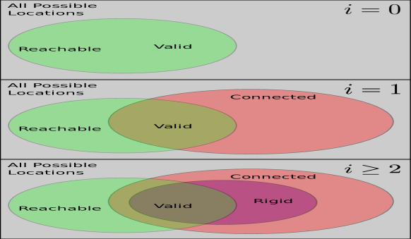
Figure 2: Visual representation of relationships between planning sets. (Top) the planning sets for AUV $0$, where all reachable locations are considered valid. (Middle) the planning sets for AUV $1$, where connectivity to AUV $0$ is enforced. (Bottom) the planning sets for all AUVs $i\geq 2$ where rigidity is enforced at every planning step.

Algorithm 1 Perform rigidity-constrained priority planning for all AUVs in a sequence

1:procedure Multi-AUV Planning

2:     $\text{trajectories}\leftarrow\emptyset$

3:     $\text{conflicts}\leftarrow\emptyset$

4:     $V_{0}\leftarrow\text{Construct Valid Sets (0)}$

5:     $i\leftarrow 0$ {AUV counter}

6:     $n\leftarrow$ number of AUVs

7:     while $i\not=n$ do

8:         $\text{trajectory, success}\leftarrow\text{Perform Planning}(i)$

9:         if success then

10:              $\text{trajectories}_{i}\leftarrow\text{trajectory}$

11:              $\text{conflict}\leftarrow\text{Construct Valid Sets}(i)$

12:              if conflict then

13:                  $\text{Clear Valid Sets}(i+1)$

14:                  $\text{Add Conflict}(i,\text{conflict})$

15:              else

16:                  $\text{Clear Conflicts}(i+1)$

17:                  $i\leftarrow(i+1)$               

18:         else

19:              $i\leftarrow(i-1)$

20:              if $i<0$ then

21:                  return $\emptyset$ {Planning Failed}                             

22:     return trajectories

The overall planning framework begins by predetermining the order of planning. The valid set for the first AUV is then immediately calculated and a path to the AUV’s target location is planned. Upon successful planning, the trajectory for the first AUV is used to determine the valid sets for the second AUV and then path planning is performed for the second AUV. This process then continues, with the trajectories of the already planned AUVs used to determine the valid sets of the next-to-be-planned AUV until planning has been performed for all AUVs in the network.

If during the valid set construction phase any valid set is found to be entirely empty, that is there is no valid location for the corresponding AUV and timestep, the time and location of the previous AUV at that time is then considered a ‘conflict’ and the path of the preceding AUV must be replanned such that it does not enter the conflict state. If planning for any AUV $i$ fails, then the planner reverts to AUV $i-1$ and the process continues. These two mechanisms, conflicts and replanning, allow for the planner to more flexibly handle poor configurations and attempt to replan based on knowledge of failed planning attempts without introducing any computational overhead in the case of successful planning.

Algorithm 2 Construct valid sets for AUV $i$ based on planning conflicts and the trajectories of the previous AUVs

1:function Construct Valid Sets($i$)

2:     $P_{i,0}\leftarrow$ AUV $i$ start location

3:     $V_{i,0}\leftarrow P_{i,0}$

4:     $t\leftarrow 0$

5:     $x\leftarrow$ goal location of AUV $i$

6:     while $x\not\in P_{i,t}$ do

7:         $N\leftarrow$ all neighbors of $V_{i,t}$

8:         $P_{i,t+1}\leftarrow(V_{0,t}\cup N)\setminus\text{conflicts}$

9:         if $i=0$ then

10:              $V_{i,t+1}\leftarrow P_{i,t+1}$

11:         else if $i=1$ then

12:              $C_{i,t+1}\leftarrow\text{Connected States}(t+1)$

13:              $V_{i,t+1}\leftarrow P_{i,t+1}\cap C_{i,t+1}$

14:         else

15:              $R_{i,t+1}\leftarrow\text{Rigid States}(t+1)$

16:              $V_{i,t+1}\leftarrow P_{i,t+1}\cap R_{i,t+1}$          

17:         if $V_{i,t+1}=\emptyset$ then

18:              $\text{loc}\leftarrow\text{Get AUV Location}(i,t+1)$

19:              $\text{conflict}\leftarrow(\text{loc, t+1})$

20:              return conflict {Returning state as conflict}          

21:         $t\leftarrow t+1$      

22:     return $V_{i}$ {Returning valid sets}

III Results and Discussion

TABLE I: Information and results from simulated experiments. Each test case represents a unique set of obstacles, goal locations, and number of AUVs in the network. We present the planning time required, the makespan of the trajectories, the average and maximum localization errors, and the percentage of the trajectory which the network was in a rigid configuration.

Test Case	Algorithm	# of AUVs	Planning Time (s)	Makespan	Avg. Localization Error	Max. Localization Error	% Rigid
1	RCGP (Ours)	8	8.911	33	0.948	3.067	100
	RRT	8	9.958	75	1.782	9.255	53
2	RCGP (Ours)	6	7.141	32	0.338	1.874	100
	RRT	6	8.315	72	1.056	11.044	75
3	RCGP (Ours)	8	7.513	27	1.033	3.124	100
	RRT	8	0.389	43	0.915	4.065	42
4	RCGP (Ours)	6	3.154	28	0.197	0.581	100
	RRT	6	0.354	46	0.392	1.445	91
5	RCGP (Ours)	20	163.0	22	1.176	2.311	100
	RRT	20	0.598	41	1.037	2.922	100

We tested our rigidity-constrained graph planning (RCGP) framework over a number of two-dimensional simulated environments with varying numbers of AUVs and obstacles. One of the tested environments and planning objectives is shown Figure 3a for reference.

III-A Implementation

We compare statistics on timing, planning, localization, and rigidity for our planning technique to a priority planning version of the rapidly-exploring random tree (RRT) algorithm in which the only planning constraint was that no two robots could occupy the same location at the same time. We also tested a fully coupled probabilistic roadmap planner but found that it was unable to complete planning for a small number of robots after ten minutes so we do not show the results. Simulations were programmed in Python and were run on an Intel i5-8300H processor. Results are shown in Table I.

To generate our planning graph we uniformly sampled the space over the environment at predetermined intervals and made edges between every sampled node and its nearest neighbors within a distance of 2 units. Such a planning graph can be seen in Figure 3b. We removed any edges that intersected obstacles in the environment. We assumed each robot to be a point robot and that there were no kinematic restrictions on a robot’s movement. To then perform planning on this graph we used a heuristic directed A* search with the Euclidean distance from a node to the goal location as the heuristic cost. We chose the minimum allowable rigidity to be 0.1, as this qualitatively appeared to provide a balance between localization quality and the consistent ability to successfully find valid trajectories.

III-B Localization

To compare the ability to localize over the course of a given path we implemented the sensor network localization approach of [7] and report both the mean error and the max error of the localization results for a given trajectory, where error is calculated as the Euclidean distance between the SNL localization results and the ground truth locations. To allow for absolute localization, as opposed to just relative, at each timestep three AUVs were randomly selected as having a known location for the purpose of SNL.

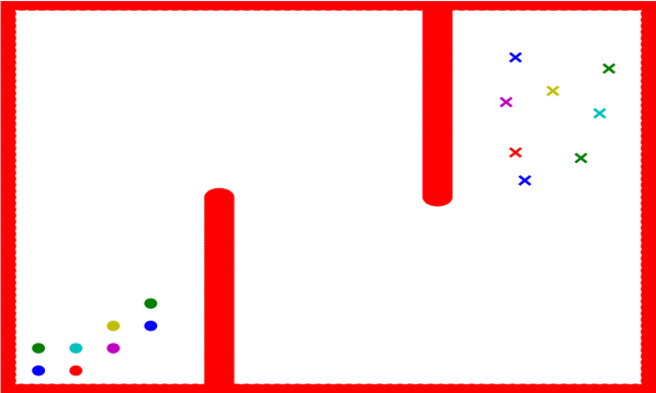
(a) Planning problem: dots are start positions and crosses are goals

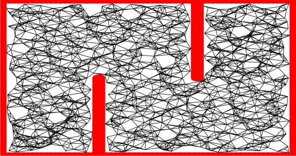
(b) Planning graph for the planning problem shown above

Figure 3: Example planning problem and corresponding planning graph. The red outlines denote obstacles to avoid. Colors are used to show correspondence between the start and goal positions for each simulated AUV

As expected, the localization results for trajectories generated by our algorithm generally had similar or reduced average localization error than the trajectories generated by the RRT algorithm. Notably, the maximum localization error for RCGP trajectories was lower in every test case, and often was a substantial amount below the maximum localization error for RRT trajectories. This would support the claim that the use of rigidity-constrained planning improves ability to perform range-only localization.

In addition, while percent time rigid is useful metric, it should be noted that this statistic still misses many important details, as there are many different qualities of non-rigidity and network configuration which all affect localizability to varying degrees. This helps explain why there is no strong relationship between percent time rigid and localization error beyond the fact that trajectories which have any amount nonrigid time appear to have increased localization errors. Additionally, it is important to note that other localization algorithms will report different localization results, though the general relationship between error and rigidity is expected to hold true.

III-C Planning

To evaluate the feasibility of each planner we report the makespan and time required to plan the full set of trajectories. The makespan is the time elapsed from the start of the trajectories to when the last AUV reaches its goal position. In the case of RGCP the planning time includes the time required to build the planning graph.

In environments with marked complexity or more challenging obstacles, notably Test Cases 1 and 2, it was found that the planning time was comparable between the two approaches and. However, in more simple environments with randomly placed obstacles and a large amount of free space the RRT was able to plan trajectories an order of magnitude faster with a moderately sized number of AUVs (Test Cases 3 and 4) and three orders of magnitude faster with a larger number of AUVs (Test Case 5). This reveals a trend of the RRT planner generally scaling linearly with the number of AUVs while the runtime of our planner does not scale as well. Profiling of our planner reveals that over ninety-nine percent of the computation of our planner is due to checking the rigidity of a location, as shown in step 15 of Algorithm 2.

Beyond planning time, we note that our RGCP algorithm finds trajectories which generally have a much reduced makespan compared to our RRT implementation. This difference between our RRT implementation and our RGCP algorithm is largely due to the use of A* to perform planning on the graph. This incentives the RGCP planner to minimize travel time. In comparison, the RRT implementation used would often generate inefficient trajectories with no weight given to the travel time. We do not compare the resulting makespans to the theoretically optimal makespan, but these results along with visual inspection of the trajectories indicate that the RGCP planner does generate time-efficient trajectories.

IV Conclusions

We were successfully able to construct a rigidity-constrained planning framework which was able to reliably plan efficient, rigidity-constrained trajectories. The results seen in Table I show that the planner is capable of planning paths for a moderate number of AUVs in a feasible amount of time while meeting a minimum network rigidity at every timestep. The use of our network rigidity measure is supported by the given localization results, which show higher localization accuracy for our planner than our RRT implementation, which does not guarantee a minimum network rigidity.

Future work in this field of rigidity-constrained planning should explore the use of precomputed formations to avoid the need for evaluating a given network’s rigidity at planning-time, as the majority of time spent in planning is on evaluating the rigidity. Furthermore, the presented priority-planning approach has two distinct drawbacks; the presented framework can eliminate valid trajectories from start to goal configurations and the quality and success of the planning is highly dependent on priority ordering. Future work to address these issues could consider other representations of the rigidity-constrained planning problem which either does not use priority-based planning or does not impose such strict planning constraints as rigidity at every step of the planning sequence.

V Acknowledgements

This work was partially supported by ONR grant N00014-18-1-2832, ONR MURI grant N00014-19-1-2571 and the MIT-Portugal program.

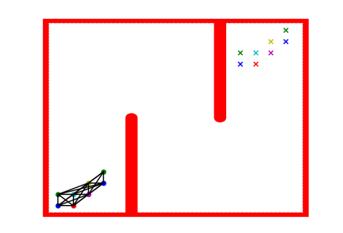
(a) Starting Position

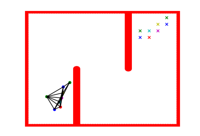
(b) Positions at timestep 5

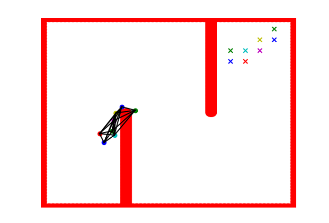
(c) Positions at timestep 10

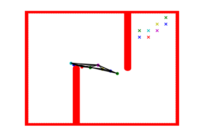
(d) Positions at timestep 15

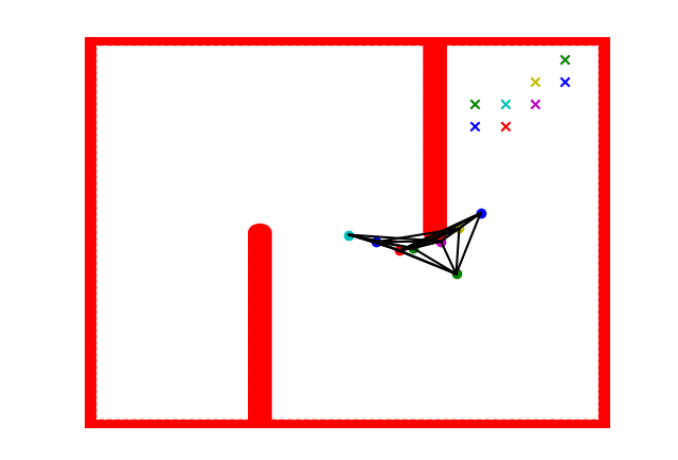
(e) Positions at timestep 20

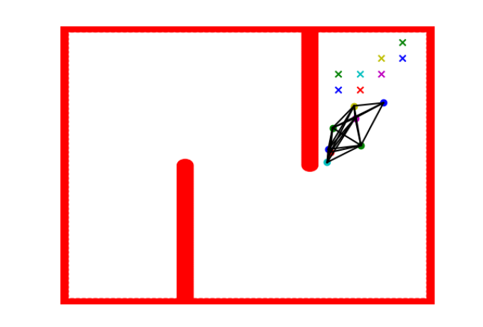
(f) Positions at timestep 25

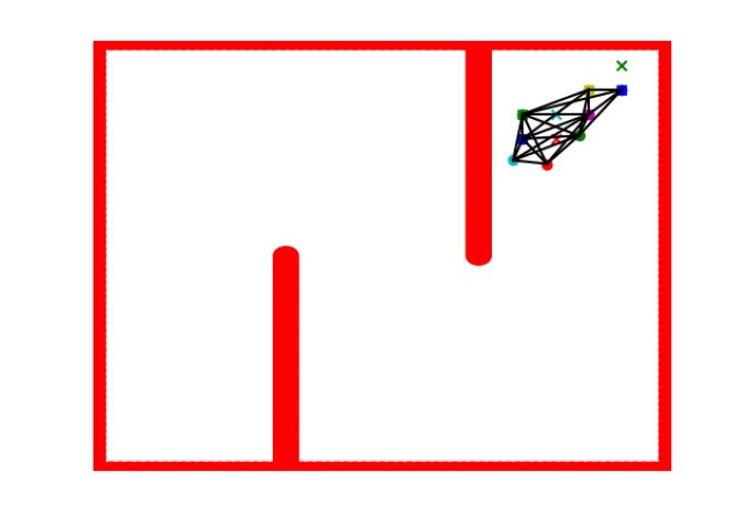
(g) Positions at timestep 30

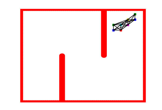
(h) Arrived at goal positions

Figure 4: Snapshots of a planned trajectory. It can be notices that in sections where a naive planner might collapse into a low-rigidity configuration (such as rounding a corner) the rigidity-constrained planner will have a small number of robots which provide triangulation for all of the others. This can be observed specifically in Figure 4b, Figure 4d, and Figure 4e

References

- [1] Liam Paull, Sajad Saeedi, Mae Seto and Howard Li “AUV navigation and localization: A review” In IEEE Journal of Oceanic Engineering 39.1 IEEE, 2014, pp. 131–149 DOI: 10.1109/JOE.2013.2278891
- [2] M.. Larsen “High performance Doppler-inertial navigation-experimental results” In OCEANS 2000 MTS/IEEE Conference and Exhibition 2, 2000, pp. 1449–1456 vol.2
- [3] N.. Rypkema and H. Schmidt “Formation Control of a Drifting Group of Marine Robotic Vehicles” In Distributed Autonomous Robotic Systems Springer International Publishing, 2018, pp. 633–647 DOI: 10.1007/978-3-319-73008-0_44
- [4] James Aspnes et al. “A theory of network localization” In IEEE Transactions on Mobile Computing 5.12 IEEE, 2006, pp. 1663–1677 DOI: 10.1109/TMC.2006.174
- [5] Erin Marie Fischell, Anne R. Kroo and Brendan W. O’Neill “Single-Hydrophone Low-Cost Underwater Vehicle Swarming” In IEEE Robotics and Automation Letters 5.2, 2020, pp. 354–361 DOI: 10.1109/LRA.2019.2958774
- [6] Giuseppe C. Calafiore, Luca Carlone and Mingzhu Wei “A distributed technique for localization of agent formations from relative range measurements” In IEEE Transactions on Systems, Man, and Cybernetics Part A:Systems and Humans 42.5, 2012, pp. 1065–1076 DOI: 10.1109/TSMCA.2012.2185045
- [7] Pratik Biswas et al. “Semidefinite programming approaches for sensor network localization with noisy distance measurements” In IEEE Transactions on Automation Science and Engineering 3.4, 2006, pp. 360–371 DOI: 10.1109/TASE.2006.877401
- [8] David Moore, John Leonard, Daniela Rus and Seth Teller “Robust distributed network localization with noisy range measurements” In SenSys’04 - Proceedings of the Second International Conference on Embedded Networked Sensor Systems, 2004, pp. 50–61 DOI: 10.1145/1031495.1031502
- [9] Jerome Le Ny and Simon Chauvière “Localizability-Constrained Deployment of Mobile Robotic Networks with Noisy Range Measurements” In Proceedings of the American Control Conference 2018-June AACC, 2018, pp. 2788–2793 DOI: 10.23919/ACC.2018.8431528
- [10] Daniel Zelazo, Antonio Franchi, Heinrich H. Bülthoff and Paolo Robuffo Giordano “Decentralized rigidity maintenance control with range measurements for multi-robot systems” In International Journal of Robotics Research 34.1, 2015, pp. 105–128 DOI: 10.1177/0278364914546173
- [11] Jur P. Van Den Berg and Mark H. Overmars “Prioritized motion planning for multiple robots” In 2005 IEEE/RSJ International Conference on Intelligent Robots and Systems, IROS, 2005, pp. 2217–2222 DOI: 10.1109/IROS.2005.1545306
- [12] Guni Sharon, Roni Stern, Ariel Felner and Nathan R Sturtevant “Conflict-based search for optimal multi-agent pathfinding” In Artificial Intelligence 219 Elsevier, 2015, pp. 40–66
- [13] Neal Patwari et al. “Locating the nodes: cooperative localization in wireless sensor networks” In IEEE Signal processing magazine 22.4 IEEE, 2005, pp. 54–69
- [14] Timothy D Barfoot “State Estimation for Robotics” Cambridge University Press, 2017
- [15] Lydia E. Kavraki, Petr Švestka, Jean Claude Latombe and Mark H. Overmars “Probabilistic roadmaps for path planning in high-dimensional configuration spaces” In IEEE Transactions on Robotics and Automation 12.4, 1996, pp. 566–580 DOI: 10.1109/70.508439