Abstract

We propose two efficient numerical approaches for solving variable-order fractional optimal control-affine problems. The variable-order fractional derivative is considered in the Caputo sense, which together with the Riemann–Liouville integral operator is used in our new techniques. An accurate operational matrix of variable-order fractional integration for Bernoulli polynomials is introduced. Our methods proceed as follows. First, a specific approximation of the differentiation order of the state function is considered, in terms of Bernoulli polynomials. Such approximation, together with the initial conditions, help us to obtain some approximations for the other existing functions in the dynamical control-affine system. Using these approximations, and the Gauss–Legendre integration formula, the problem is reduced to a system of nonlinear algebraic equations. Some error bounds are then given for the approximate optimal state and control functions, which allow us to obtain an error bound for the approximate value of the performance index. We end by solving some test problems, which demonstrate the high accuracy of our results.

Submitted: September 4, 2020; Revised: October 4, 2020; Accepted: October 6, 2020 Application of Bernoulli Polynomials for Solving Variable-Order Fractional Optimal Control-Affine Problems Somayeh Nemati ¹, Delfim F. M. Torres ²* Somayeh Nemati and Delfim F. M. Torres Correspondence: delfim@ua.pt; Tel.: +351-234-370-668 34A08; 65M70 (Primary); 11B68 (Secondary)

1 Introduction

The Bernoulli polynomials, named after Jacob Bernoulli (1654–1705), occur in the study of many special functions and, in particular, in relation with fractional calculus, which is a classical area of mathematical analysis whose foundations were laid by Liouville in a paper from 1832 and that is nowadays a very active research area Machado et al. (2011). One can say that Bernoulli polynomials are a powerful mathematical tool in dealing with various problems of dynamical nature Keshavarz et al. (2016); Bhrawy et al. (2012); Tohidi et al. (2013); Toutounian and Tohidi (2013); Bazm (2015). Recently, an approximate method, based on orthonormal Bernoulli’s polynomials, has been developed for solving fractional order differential equations of Lane–Emden type Sahu and Mallick (2019), while in Loh and Phang (2019) Bernoulli polynomials are used to numerical solve Fredholm fractional integro-differential equations with right-sided Caputo derivatives. Here we are interested in the use of Bernoulli polynomials with respect to fractional optimal control problems.

An optimal control problem refers to the minimization of a functional on a set of control and state variables (the performance index) subject to dynamic constraints on the states and controls. When such dynamic constraints are described by fractional differential equations, then one speaks of fractional optimal control problems (FOCPs) Rosa and Torres (2018). The mathematical theory of fractional optimal control has born in 1996/97 from practical problems of mechanics and began to be developed in the context of the fractional calculus of variations Malinowska and Torres (2012); Malinowska et al. (2015); Almeida et al. (2015). Soon after, fractional optimal control theory became a mature research area, supported with many applications in engineering and physics. For the state of the art, see Ali et al. (2019); Nemati et al. (2019); Salati et al. (2019) and references therein. Regarding the use of Bernoulli polynomials to numerically solve FOCPs, we refer to Keshavarz et al. (2016), where the operational matrices of fractional Riemann–Liouville integration for Bernoulli polynomials are derived and the properties of Bernoulli polynomials are utilized, together with Newton’s iterative method, to find approximate solutions to FOCPs. The usefulness of Bernoulli polynomials for mixed integer-fractional optimal control problems is shown in Rabiei et al. (2018), while the practical relevance of the methods in engineering is illustrated in Behroozifar and Habibi (2018). Recently, such results have been generalized for two-dimensional fractional optimal control problems, where the control system is not a fractional ordinary differential equation but a fractional partial differential equation Rahimkhani and Ordokhani (2019). Here we are the first to develop a numerical method, based on Bernoulli polynomials, for FOCPs of variable-order.

The variable-order fractional calculus was introduced in 1993 by Samko and Ross and deals with operators of order $\alpha$, where $\alpha$ is not necessarily a constant but a function $\alpha(t)$ of time Samko and Ross (1993). With this extension, numerous applications have been found in physics, mechanics, control, and signal processing Lorenzo and Hartley (2002); Abdeljawad et al. (2019); Hassani and Naraghirad (2019); Odzijewicz et al. (2013); Yan et al. (2019). For the state of the art on variable-order fractional optimal control we refer the interested reader to the book Almeida et al. (2019) and the articles Heydari and Avazzadeh (2018); Mohammadi and Hassani (2019). To the best of our knowledge, numerical methods based on Bernoulli polynomials for such kind of FOCPs are not available in the literature. For this reason, in this work we focus on the following variable-order fractional optimal control-affine problem (FOC-AP):

$$\min~{}J=\int_{0}^{1}\phi(t,x(t),u(t))dt$$ (1)

subject to the control-affine dynamical system

$${{}_{0}^{C}D}_{t}^{\alpha(t)}x(t)=\varphi\left(t,x(t),{{}_{0}^{C}D}_{t}^{\alpha_{1}(t)}x(t),\dots,{{}_{0}^{C}D}_{t}^{\alpha_{s}(t)}x(t)\right)+b(t)u(t)$$ (2)

and the initial conditions

$$x^{(i)}(0)=x_{0}^{i},\quad i=0,1,\ldots,n,$$ (3)

where $\phi$ and $\varphi$ are smooth functions of their arguments, $b\neq 0$, $n$ is a positive integer number such that for all $t\in[0,1]$, $0<\alpha_{1}(t)<\alpha_{2}(t)<\ldots<\alpha_{s}(t)<\alpha(t)\leq n$, and ${{}_{0}^{C}D_{t}^{\alpha(t)}}$ is the (left) fractional derivative of variable-order defined in the Caputo sense. We employ two spectral methods based on Bernoulli polynomials in order to obtain numerical solutions to problem (1)–(3). Our main idea consists of reducing the problem to a system of nonlinear algebraic equations. To do this, we introduce an accurate operational matrix of variable-order fractional integration, having Bernoulli polynomials as basis vectors.

The paper is organized as follows. In Section 2, the variable-order fractional calculus is briefly reviewed and some properties of the Bernoulli polynomials are recalled. A new operational matrix of variable-order is introduced for the Bernoulli basis functions in Section 3. Section 4 is devoted to two new numerical approaches based on Bernoulli polynomials for solving problem (1)–(3). In Section 5, some error bounds are proved. Then, in Section 6, some FOC-APs are solved using the proposed methods. Finally, concluding remarks are given in Section 7.

2 Preliminaries

In this section, a brief review on necessary definitions and properties of the variable-order fractional calculus is presented. Furthermore, Bernoulli polynomials and some of their properties are recalled.

2.1 The variable-order fractional calculus

The two most commonly used definitions in fractional calculus are the Riemann–Liouville integral and the Caputo derivative. Here, we deal with generalizations of these two definitions, which allow the order of the fractional operators to be of variable-order.

[See, e.g., Almeida et al. (2019)] The left Riemann–Liouville fractional integral of order $\alpha(t)$ is defined by

$${}_{0}I_{t}^{\alpha(t)}y(t)=\frac{1}{\Gamma{(\alpha(t))}}\int_{0}^{t}(t-s)^{\alpha(t)-1}y(s)ds,\quad t>0,$$

where $\Gamma$ is the Euler gamma function, that is,

$$\Gamma(t)=\int_{0}^{\infty}\tau^{t-1}\exp(-\tau)d\tau,\quad t>0.$$

[See, e.g., Almeida et al. (2019)] The left Caputo fractional derivative of order $\alpha(t)$ is defined by

$${{}_{0}^{C}D}_{t}^{\alpha(t)}y(t)=\frac{1}{\Gamma(n-\alpha(t))}\int_{0}^{t}(t-s)^{n-\alpha(t)-1}y^{(n)}(s)ds,\quad n-1<\alpha(t)<n,$$

$${{}_{0}^{C}D}_{t}^{\alpha(t)}y(t)=y^{(n)}(t),\quad\alpha(t)=n.$$

For $0\leq\beta(t)<\alpha(t)\leq n$, $n\in\mathbb{N}$, $\gamma>0$, and $\nu>-1$, some useful properties of the Caputo derivative and Riemann–Liouville fractional integral are as follows Almeida et al. (2019):

$$_{0}I_{t}^{\alpha(t)}t^{\nu}=\frac{\Gamma(\nu+1)}{\Gamma{(\nu+1+\alpha(t))}}t^{\nu+\alpha(t)},$$ (4)

$$_{0}I_{t}^{\gamma}({{}_{0}^{C}D}_{t}^{\gamma}y(t))=y(t)-\sum_{i=0}^{\lceil\gamma\rceil-1}y^{(i)}(0)\frac{t^{i}}{i!},\quad t>0,$$ (5)

$$_{0}I_{t}^{n-\alpha(t)}(y^{(n)}(t))={{}_{0}^{C}D}_{t}^{\alpha(t)}y(t)-\sum_{i=\lceil\alpha(t)\rceil}^{n-1}y^{(i)}(0)\frac{t^{i-\alpha(t)}}{\Gamma(i+1-\alpha(t))},\quad t>0,$$ (6)

$$_{0}I_{t}^{\alpha(t)-\beta(t)}({{}_{0}^{C}D}_{t}^{\alpha(t)}y(t))={{}_{0}^{C}D}_{t}^{\beta(t)}y(t)-\sum_{i=\lceil\beta(t)\rceil}^{\lceil\alpha(t)\rceil-1}y^{(i)}(0)\frac{t^{i-\beta(t)}}{\Gamma(i+1-\beta(t))},\quad t>0,$$ (7)

where $\lceil\cdot\rceil$ is the ceiling function.

2.2 Bernoulli polynomials

The set of Bernoulli polynomials, $\{\beta_{m}(t)\}_{m=0}^{\infty}$, consists of a family of independent functions that builds a complete basis for the space $L^{2}[0,1]$ of all square integrable functions on the interval $[0,1]$. These polynomials are defined as

$$\beta_{m}(t)=\sum_{i=0}^{m}\binom{m}{i}b_{m-i}t^{i},$$ (8)

where $b_{k}$, $k=0,1,\ldots,m$, are the Bernoulli numbers Costabile et al. (2006). These numbers are seen in the series expansion of trigonometric functions and can be given by the following identity Arfken (1966):

$$\frac{t}{e^{t}-1}=\sum_{i=0}^{\infty}b_{i}\frac{t^{i}}{i!}.$$

Thus, the first few Bernoulli numbers are given by

$$b_{0}=1,\quad b_{1}=-\frac{1}{2},\quad b_{2}=\frac{1}{6},\quad b_{3}=0,\quad b_{4}=-\frac{1}{30},\quad b_{5}=0,\quad b_{6}=\frac{1}{42}.$$

Furthermore, the first five Bernoulli polynomials are

$$\beta_{0}(t)=1,$$

$$\beta_{1}(t)=t-\frac{1}{2},$$

$$\beta_{2}(t)=t^{2}-t+\frac{1}{6},$$

$$\beta_{3}(t)=t^{3}-\frac{3}{2}t^{2}+\frac{1}{2}t,$$

$$\beta_{4}(t)=t^{4}-2t^{3}+t^{2}-\frac{1}{30}.$$

For an arbitrary function $x\in L^{2}[0,1]$, we can write

$$x(t)=\sum_{m=0}^{\infty}a_{m}\beta_{m}(t).$$

Therefore, an approximation of the function $x$ can be given by

$$x(t)\simeq x_{M}(t)=\sum_{m=0}^{M}a_{m}\beta_{m}(t)=A^{T}B(t),$$ (9)

where

$$B(t)=[\beta_{0}(t),\beta_{1}(t),\ldots,\beta_{M}(t)]^{T}$$ (10)

and

$$A=[a_{0},a_{1},\ldots,a_{M}]^{T}.$$

The vector $A$ in (9) is called the coefficient vector and can be calculated by the formula (see Keshavarz et al. (2016))

$$A=D^{-1}\langle x(t),B(t)\rangle,$$

where $\langle\cdot,\cdot\rangle$ is the inner product, defined for two arbitrary functions $f,g\in L^{2}[0,1]$ as

$$\langle f(t),g(t)\rangle=\int_{0}^{1}f(t)g(t)dt,$$

and $D=\langle B(t),B(t)\rangle$ is calculated using the following property of Bernoulli polynomials Arfken (1966):

$$\int_{0}^{1}\beta_{i}(t)\beta_{j}(t)dt=(-1)^{i-1}\frac{i!j!}{(i+j)!}b_{i+j},\quad i,j\geq 1.$$

It should be noted that

$$X=span\left\{\beta_{0}(t),\beta_{1}(t),\ldots,\beta_{M}(t)\right\}$$

is a finite dimensional subspace of $L^{2}[0,1]$ and $x_{M}$, given by (9), is the best approximation of function $x$ in $X$.

3 Operational matrix of variable-order fractional integration

In this section, we introduce an accurate operational matrix of variable-order fractional integration for Bernoulli functions. To this aim, we rewrite the Bernoulli basis vector $B$ given by (10) in terms of the Taylor basis functions as follows:

$$B(t)=Q\mathbb{T}(t),$$ (11)

where $\mathbb{T}$ is the Taylor basis vector given by

$$\mathbb{T}(t)=\left[1,t,t^{2},\ldots,t^{M}\right]^{T}$$

and $Q$ is the change-of-basis matrix, which is obtained using (8) as

$$Q=\left[\begin{array}[]{ccccccc}1&0&0&0&0&\ldots&0\\ -\frac{1}{2}&1&0&0&0&\ldots&0\\ \frac{1}{6}&-1&1&0&0&\ldots&0\\ 0&\frac{1}{2}&-\frac{3}{2}&1&0&\ldots&0\\ \vdots&\vdots&\vdots&\vdots&\vdots&&\vdots\\ b_{M}&\binom{M}{1}b_{M-1}&\binom{M}{2}b_{M-2}&\binom{M}{3}b_{M-3}&\binom{M}{4}b_{M-4}&\ldots&1\\ \end{array}\right].$$

Since $Q$ is nonsingular, we can write

$$\mathbb{T}(t)=Q^{-1}B(t).$$ (12)

By considering (11) and applying the left Riemann–Liouville fractional integral operator of order $\alpha(t)$ to the vector $B(t)$, we get that

$$_{0}I_{t}^{\alpha(t)}B(t)={{}_{0}I_{t}^{\alpha(t)}}(Q\mathbb{T}(t))=Q({{}_{0}I_{t}^{\alpha(t)}}\mathbb{T}(t))=QS_{t}^{\alpha(t)}\mathbb{T}(t),$$ (13)

where $S_{t}^{\alpha(t)}$ is a diagonal matrix, which is obtained using (4) as follows:

$$S_{t}^{\alpha(t)}=\left[\begin{array}[]{cccccc}\frac{1}{\Gamma(1+\alpha(t))}t^{\alpha(t)}&0&0&0&\cdots&0\\ 0&\frac{1}{\Gamma(2+\alpha(t))}t^{\alpha(t)}&0&0&\cdots&0\\ 0&0&\frac{2}{\Gamma(3+\alpha(t))}t^{\alpha(t)}&0&\cdots&0\\ \vdots&\vdots&\vdots&\vdots&&\vdots\\ 0&0&0&0&\cdots&\frac{\Gamma(M+1)}{\Gamma{(M+1+\alpha(t))}}t^{\alpha(t)}\\ \end{array}\right].$$

Finally, by using (12) in (13), we have

$$_{0}I_{t}^{\alpha(t)}B(t)=QS_{t}^{\alpha(t)}Q^{-1}B(t)=P_{t}^{\alpha(t)}B(t),$$ (14)

where $P_{t}^{\alpha(t)}=QS_{t}^{\alpha(t)}Q^{-1}$ is a matrix of dimension $(M+1)\times(M+1)$, which we call the operational matrix of variable-order fractional integration $\alpha(t)$ for Bernoulli functions. Since $Q$ and $Q^{-1}$ are lower triangular matrices and $S_{t}^{\alpha(t)}$ is a diagonal matrix, $P_{t}^{\alpha(t)}$ is also a lower triangular matrix. In the particular case of $M=2$, one has

$$P_{t}^{\alpha(t)}=\left[\begin{array}[]{ccc}\frac{1}{\Gamma(\alpha(t)+1)}t^{\alpha(t)}&0&0\\ \left(\frac{1}{2\Gamma(\alpha(t)+2)}-\frac{1}{2\Gamma(\alpha(t)+1)}\right)t^{\alpha(t)}&\frac{1}{\Gamma(\alpha(t)+2)}t^{\alpha(t)}&0\\ \left(\frac{1}{6\Gamma(\alpha(t)+1)}-\frac{1}{2\Gamma(\alpha(t)+2)}+\frac{2}{3\Gamma(\alpha(t)+3)}\right)t^{\alpha(t)}&\left(\frac{2}{\Gamma(\alpha(t)+3)}-\frac{1}{\Gamma(\alpha(t)+2)}\right)t^{\alpha(t)}&\frac{2}{\Gamma(\alpha(t)+3)}t^{\alpha(t)}\end{array}\right].$$

4 Methods of solution

In this section, we propose two approaches for solving problem (1)–(3). To do this, first we introduce

$$n=\max_{0<t\leq 1}\left\{\lceil\alpha(t)\rceil\right\}.$$

Then, we may use the following two approaches to find approximations for the state and control functions, which optimize the performance index.

4.1 Approach I

In our first approach, we consider an approximation of the $n$th order derivative of the unknown state function $x$ using Bernoulli polynomials. Set

$$x^{(n)}(t)=A^{T}B(t),$$ (15)

where $A$ is a $1\times(M+1)$ vector with unknown elements and $B$ is the Bernoulli basis vector given by (10). Then, using the initial conditions given in (3), and equations (5), (14), and (15), we get

$$\begin{split}x(t)&={{}_{0}I_{t}^{n}}(x^{(n)}(t))+\sum_{i=0}^{n-1}x^{(i)}(0)\frac{t^{i}}{i!}\\ &=A^{T}({{}_{0}I_{t}^{n}}B(t))+\sum_{i=0}^{n-1}x_{0}^{i}\frac{t^{i}}{i!}\\ &=A^{T}P_{t}^{n}B(t)+\sum_{i=0}^{n-1}x_{0}^{i}\frac{t^{i}}{i!}.\end{split}$$ (16)

Moreover, using (6), (14), and (15), we get

$${{}_{0}^{C}D}_{t}^{\alpha(t)}x(t)=A^{T}P_{t}^{n-\alpha(t)}B(t)+\sum_{i=\lceil\alpha(t)\rceil}^{n-1}x_{0}^{i}\frac{t^{i-\alpha(t)}}{\Gamma(i+1-\alpha(t))}:=F[A,t]$$ (17)

and

$${{}_{0}^{C}D}_{t}^{\alpha_{j}(t)}x(t)=A^{T}P_{t}^{n-\alpha_{j}(t)}B(t)+\sum_{i=\lceil\alpha_{j}(t)\rceil}^{n-1}x_{0}^{i}\frac{t^{i-\alpha_{j}(t)}}{\Gamma(i+1-\alpha_{j}(t))}:=F_{j}[A,t],\quad j=1,\ldots,s.$$ (18)

By substituting (16)–(18) into the control-affine dynamical system given by (2), we obtain an approximation of the control function as follows:

$$u(t)=\frac{1}{b(t)}\left[F[A,t]-\varphi\left(t,A^{T}P_{t}^{n}B(t)+\sum_{i=0}^{n-1}x_{0}^{i}\frac{t^{i}}{i!},F_{1}[A,t],\dots,F_{s}[A,t]\right)\right].$$ (19)

Taking into consideration (16) and (19) in the performance index $J$, we have

$$J[A]=\int_{0}^{1}{\phi\left(t,A^{T}P_{t}^{n}B(t)+\sum_{i=0}^{n-1}x_{0}^{i}\frac{t^{i}}{i!},\frac{1}{b(t)}\left[F[A,t]-\varphi\left(t,A^{T}P_{t}^{n}B(t)+\sum_{i=0}^{n-1}x_{0}^{i}\frac{t^{i}}{i!},F_{1}[A,t],\dots,F_{s}[A,t]\right)\right]\right)dt}.$$

For the sake of simplicity, we introduce

$$G[A,t]=\phi\left(t,A^{T}P_{t}^{n}B(t)+\sum_{i=0}^{n-1}x_{0}^{i}\frac{t^{i}}{i!},\frac{1}{b(t)}\left[F[A,t]-\varphi\left(t,A^{T}P_{t}^{n}B(t)+\sum_{i=0}^{n-1}x_{0}^{i}\frac{t^{i}}{i!},F_{1}[A,t],\dots,F_{s}[A,t]\right)\right]\right).$$

In many applications, it is difficult to compute the integral of function $G[A,t]$. Therefore, it is recommended to use a suitable numerical integration formula. Here, we use the Gauss–Legendre quadrature formula to obtain

$$J[A]\simeq\frac{1}{2}\sum_{i=1}^{N}\omega_{i}G\left[A,\frac{t_{i}+1}{2}\right],$$ (20)

where $t_{i}$, $i=1,2,\ldots,N$, are the zeros of the Legendre polynomial of degree $N$, $P_{N}(t)$, and $\omega_{i}$ are the corresponding weights Shen et al. (2011), which are given by

$$\omega_{i}=\frac{2}{\left(\frac{d}{dt}P_{N}(t_{i})\right)^{2}(1-t_{i}^{2})},\quad i=1,\ldots,N.$$ (21)

Finally, the first order necessary condition for the optimality of the performance index implies

$$\frac{\partial J[A]}{\partial A}=0,$$

which gives a system of $M+1$ nonlinear algebraic equations in terms of the $M+1$ unknown elements of the vector $A$. By solving this system, approximations of the optimal state and control functions are, respectively, given by (16) and (19).

4.2 Approach II

In our second approach, we set

$${{}_{0}^{C}D}_{t}^{\alpha(t)}x(t)=A^{T}B(t).$$ (22)

Then, using (7) with $\beta(t)\equiv 0$, we obtain that

$$\begin{split}x(t)&={{}_{0}I_{t}^{\alpha(t)}}({{}_{0}^{C}D}_{t}^{\alpha(t)}x(t))+\sum_{i=0}^{\lceil\alpha(t)\rceil-1}x^{(i)}(0)\frac{t^{i}}{\Gamma(i+1)}\\ &=A^{T}({{}_{0}I_{t}^{\alpha(t)}}B(t))+\sum_{i=0}^{\lceil\alpha(t)\rceil-1}x_{0}^{i}\frac{t^{i}}{i!}\\ &=A^{T}P_{t}^{\alpha(t)}B(t)+\sum_{i=0}^{\lceil\alpha(t)\rceil-1}x_{0}^{i}\frac{t^{i}}{i!}.\end{split}$$ (23)

Furthermore, we get

$${{}_{0}^{C}D}_{t}^{\alpha_{j}(t)}x(t)=A^{T}P_{t}^{\alpha(t)-\alpha_{j}(t)}B(t)+\sum_{i=\lceil\alpha_{j}(t)\rceil}^{\lceil\alpha(t)\rceil-1}x_{0}^{i}\frac{t^{i-\alpha_{j}(t)}}{\Gamma(i+1-\alpha_{j}(t))}:=F_{j}[A,t],\quad j=1,\ldots,s.$$ (24)

Taking (22)–(24) into consideration, equation (2) gives

$$u(t)=\frac{1}{b(t)}\left[A^{T}B(t)-\varphi\left(t,A^{T}P_{t}^{\alpha(t)}B(t)+\sum_{i=0}^{\lceil\alpha(t)\rceil-1}x_{0}^{i}\frac{t^{i}}{i!},F_{1}[A,t],\dots,F_{s}[A,t]\right)\right].$$ (25)

By substituting the approximations given by (23) and (25) into the performance index, we get

$$J[A]=\int_{0}^{1}\phi\left(t,A^{T}P_{t}^{\alpha(t)}B(t)+\sum_{i=0}^{\lceil\alpha(t)\rceil-1}x_{0}^{i}\frac{t^{i}}{i!},\right.\\ \left.\frac{1}{b(t)}\left[A^{T}B(t)-\varphi\left(t,A^{T}P_{t}^{\alpha(t)}B(t)+\sum_{i=0}^{\lceil\alpha(t)\rceil-1}x_{0}^{i}\frac{t^{i}}{i!},F_{1}[A,t],\dots,F_{s}[A,t]\right)\right]\right)dt.$$

By introducing

$$G[A,t]=\phi\left(t,A^{T}P_{t}^{\alpha(t)}B(t)+\sum_{i=0}^{\lceil\alpha(t)\rceil-1}x_{0}^{i}\frac{t^{i}}{i!},\right.\\ \left.\frac{1}{b(t)}\left[A^{T}B(t)-\varphi\left(t,A^{T}P_{t}^{\alpha(t)}B(t)+\sum_{i=0}^{\lceil\alpha(t)\rceil-1}x_{0}^{i}\frac{t^{i}}{i!},F_{1}[A,t],\dots,F_{s}[A,t]\right)\right]\right),$$

then this approach continues in the same way of finding the unknown parameters of the vector $A$ as in Approach I.

5 Error bounds

The aim of this section is to give some error bounds for the numerical solution obtained by the proposed methods of Section 4. We present the error discussion for Approach II, which can then be easily extended to Approach I.

Suppose that $x^{*}$ is the optimal state function of problem (1)–(3). Let $f(t):={{}_{0}^{C}D}_{t}^{\alpha(t)}x^{*}(t)$ with $f(t)\in H^{\mu}(0,1)$ ($H^{\mu}(0,1)$ is a Sobolev space Canuto et al. (2006)). According to our numerical method, $f_{M}(t)=A^{T}B(t)$ is the best approximation of function $f$ in terms of the Bernoulli polynomials, that is,

$$\forall g\in X,~{}\|f-f_{M}\|_{2}\leq\|f-g\|_{2}.$$

We recall the following lemma from Canuto et al. (2006).

[See Canuto et al. (2006)] Assume that $f\in H^{\mu}(0,1)$ with $\mu\geq 0$. Let $L_{M}(f)\in X$ be the truncated shifted Legendre series of $f$. Then,

$$\|f-L_{M}(f)\|_{2}\leq CM^{-\mu}|f|_{H^{\mu;M}(0,1)},$$

where

$$|f|_{H^{\mu;M}(0,1)}=\left(\sum_{j=\min\{\mu,M+1\}}^{\mu}\|f^{(j)}\|_{2}^{2}\right)^{\frac{1}{2}}$$

and $C$ is a positive constant independent of function $f$ and integer $M$.

Since the best approximation of function $f$ in the subspace $X$ is unique and $f_{M}$ and $L_{M}(f)$ are both the best approximations of $f$ in $X$, we have $f_{M}=L_{M}(f)$. Therefore, we get that

$$\|f-f_{M}\|_{2}\leq CM^{-\mu}|f|_{H^{\mu;M}(0,1)}.$$ (26)

Hereafter, $C$ denotes a positive constant independent of $M$ and $n$.

Suppose $x^{*}$ to be the exact optimal state function of problem (1)–(3) such that $f(t):={{}_{0}^{C}D}_{t}^{\alpha(t)}x^{*}(t)\in H^{\mu}(0,1)$, with $\mu\geq 0$, and $\tilde{x}$ be its approximation given by (23). Then,

$$\|x^{*}(t)-\tilde{x}(t)\|_{2}\leq CM^{-\mu}|f|_{H^{\mu;M}(0,1)}.$$ (27)

Proof.

Let $Y=L^{2}[0,1]$ and ${}_{0}I_{t}^{\alpha(t)}:Y\rightarrow Y$ be the variable-order Riemann–Liouville integral operator. By definition of the norm for operators, we have

$$\|_{0}I_{t}^{\alpha(t)}\|_{2}=\sup_{\|g\|_{2}=1}\|_{0}I_{t}^{\alpha(t)}g\|_{2}.$$

In order to prove the theorem, first we show that the operator ${}_{0}I_{t}^{\alpha(t)}$ is bounded. Since $\|g\|_{2}=1$, using Schwarz’s inequality, we get

$$\left\|{}_{0}I_{t}^{\alpha(t)}g\right\|_{2} =\left\|\frac{1}{\Gamma(\alpha(t))}\int_{0}^{t}(t-s)^{\alpha(t)-1}g(s)ds\right\|_{2}$$

$$\leq\|g\|_{2}\left\|\frac{1}{\Gamma(\alpha(t))}\int_{0}^{t}(t-s)^{\alpha(t)-1}ds\right\|_{2}$$

$$=\left\|\frac{t^{\alpha(t)}}{\Gamma(\alpha(t)+1)}\right\|_{2}$$

$$\leq C,$$

where we have used the assumption $\alpha(t)>0$, which gives $t^{\alpha(t)}<1$ for $0<t\leq 1$, and a particular property of the Gamma function, which is $\Gamma(t)>0.8$. Therefore, ${}_{0}I_{t}^{\alpha(t)}$ is bounded. Now, using (26), and taking into account (7) and (23), we obtain that

$$\left\|x^{*}(t)-\tilde{x}(t)\right\|_{2} =\left\|{{}_{0}I_{t}^{\alpha(t)}}f(t)+\sum_{i=0}^{\lceil\alpha(t)\rceil-1}x^{(i)}(0)\frac{t^{i}}{\Gamma(i+1)}-\left({{}_{0}I_{t}^{\alpha(t)}}(A^{T}B(t))+\sum_{i=0}^{\lceil\alpha(t)\rceil-1}x_{0}^{i}\frac{t^{i}}{i!}\right)\right\|_{2}$$

$$=\left\|{{}_{0}I_{t}^{\alpha(t)}}(f(t)-A^{T}B(t))\right\|_{2}$$

$$~{}\leq\left\|{{}_{0}I_{t}^{\alpha(t)}}\right\|_{2}\left\|f(t)-A^{T}B(t)\right\|_{2}$$

$$\leq CM^{-\mu}|f|_{H^{\mu;M}(0,1)}.$$

The proof is complete. ∎

Since we have $\alpha(t)-\alpha_{j}(t)>0$, $j=1,2,\ldots,s$, with a similar argument it can be shown that

$$\left\|{{}_{0}^{C}D}_{t}^{\alpha_{j}(t)}x^{*}(t)-\left(A^{T}P_{t}^{\alpha(t)-\alpha_{j}(t)}B(t)+\sum_{i=\lceil\alpha_{j}(t)\rceil}^{\lceil\alpha(t)\rceil-1}x_{0}^{i}\frac{t^{i-\alpha_{j}(t)}}{\Gamma(i+1-\alpha_{j}(t))}\right)\right\|_{2}\leq CM^{-\mu}|f|_{H^{\mu;M}(0,1)}.$$

With the help of Theorem 5, we obtain the following result for the error of the optimal control function. For simplicity, suppose that in the control-affine dynamical system given by (2) the function $\varphi$ appears as $\varphi:=\varphi(t,x)$ (cf. Remark 5).

Suppose that the assumptions of Theorem 5 are fulfilled. Let $u^{*}$ and $\tilde{u}$ be the exact and approximate optimal control functions, respectively. If $\varphi:\mathbb{R}^{2}\longrightarrow\mathbb{R}$ satisfies a Lipschitz condition with respect to the second argument, then

$$\|u^{*}(t)-\tilde{u}(t)\|_{2}\leq CM^{-\mu}|f|_{H^{\mu;M}(0,1)}.$$ (28)

Proof.

Using equation (2), the exact optimal control function is given by

$$u^{*}(t)=\frac{1}{b(t)}\left(f(t)-\varphi\left(t,x^{*}(t)\right)\right)$$ (29)

and the approximate control function obtained by our Approach II is given by

$$\tilde{u}(t)=\frac{1}{b(t)}\left(A^{T}B(t)-\varphi\left(t,\tilde{x}(t)\right)\right).$$ (30)

By subtracting (30) from (29), we get

$$u^{*}(t)-\tilde{u}(t)=\frac{1}{b(t)}\left(f(t)-\varphi\left(t,x^{*}(t)\right)-A^{T}B(t)+\varphi\left(t,\tilde{x}(t)\right)\right).$$ (31)

Since the function $\varphi$ satisfies a Lipschitz condition with respect to the second variable, there exists a positive constant $K$ such that

$$|\varphi(t,{\bf x}_{1})-\varphi(t,{\bf x}_{2})|<K|{\bf x}_{1}-{\bf x}_{2}|.$$

Therefore, using (26) and (27), and also taking into account $b(t)\neq 0$, we have

$$\|u^{*}(t)-\tilde{u}(t)\|_{2}\leq\frac{1}{\|b(t)\|_{2}}\left(\left\|f(t)-A^{T}B(t)\right\|_{2}+K\left\|x^{*}(t)-\tilde{x}(t)\right\|_{2}\right)\leq CM^{-\mu}|f|_{H^{\mu;M}(0,1)},$$

which yields (28). ∎

For the general case $\varphi:=\varphi(t,x,x_{1},\ldots,x_{s})$, the same result of Theorem 5 can be easily obtained by assuming that $\varphi$ satisfies Lipschitz conditions with respect to the variables $x$, $x_{1}$, …, $x_{s}$.

As a result of Theorems 5 and 5, we obtain an error bound for the approximate value of the optimal performance index $J$ given by (20). First, we recall the following lemma in order to obtain the error of the Gauss–Legendre quadrature rule.

[See Shen et al. (2011)] Let $g$ be a given sufficiently smooth function. Then, the Gauss–Legendre quadrature rule is given by

$$\int_{-1}^{1}g(t)dt=\sum_{i=1}^{N}\omega_{i}g(t_{i})+E_{N}(g),$$ (32)

where $t_{i}$, $i=1,\ldots,N$, are the roots of the Legendre polynomial of degree $N$, and $\omega_{i}$ are the corresponding weights given by (21). In (32), $E_{N}(g)$ is the error term, which is given as follows:

$$E_{N}(g)=\frac{2^{2N+1}(N!)^{4}}{(2N+1)[(2N!)]^{3}}g^{2N}(\eta),\quad\eta\in(-1,1).$$

Now, by considering the assumptions of Theorems 5 and 5, we prove the following result.

Let $J^{*}$ be the exact value of the optimal performance index $J$ in problem (1)–(3) and $\tilde{J}$ be its approximation given by (20). Suppose that the function $\phi:\mathbb{R}^{3}\longrightarrow\mathbb{R}$ is a sufficiently smooth function with respect to all its variables and satisfies Lipschitz conditions with respect to its second and third arguments, that is,

$$|\phi(t,{\bf x}_{1},u)-\phi(t,{\bf x}_{2},u)|\leq K_{1}|{\bf x}_{1}-{\bf x}_{2}|$$ (33)

and

$$|\phi(t,x,{\bf u}_{1})-\phi(t,x,{\bf u}_{2})|\leq K_{1}|{\bf u}_{1}-{\bf u}_{2}|,$$ (34)

where $K_{1}$ and $K_{2}$ are real positive constants. Then, there exist positive constants $C_{1}$ and $C_{2}$ such that

$$\left|J^{*}-\tilde{J}\right|\leq C_{1}M^{-\mu}|f|_{H^{\mu;M}(0,1)}+C_{2}\frac{(N!)^{4}}{(2N+1)[(2N!)]^{3}}.$$ (35)

Proof.

Using (20) and (32), we have

$$\tilde{J}=\frac{1}{2}\sum_{i=1}^{N}\omega_{i}\phi\left(\frac{t_{i}+1}{2},\tilde{x}\left(\frac{t_{i}+1}{2}\right),\tilde{u}\left(\frac{t_{i}+1}{2}\right)\right)=\int_{0}^{1}\phi\left(t,\tilde{x}(t),\tilde{u}(t)\right)dt-\xi_{N},$$ (36)

where

$$\xi_{N}=\left(\frac{1}{2}\right)\frac{2^{2N+1}(N!)^{4}}{(2N+1)[(2N!)]^{3}}\left(\frac{1}{2}\right)^{2N}\left.\frac{\partial^{2N}\phi\left(t,\tilde{x}(t),\tilde{u}(t)\right)}{\partial t^{2N}}\right|_{t=\eta}=\frac{(N!)^{4}}{(2N+1)[(2N!)]^{3}}\left.\frac{\partial^{2N}\phi\left(t,\tilde{x}(t),\tilde{u}(t)\right)}{\partial t^{2N}}\right|_{t=\eta}$$

for $\eta\in(0,1)$. Therefore, taking into consideration (33)–(36), we get

$$\left|J^{*}-\tilde{J}\right| =\left|\int_{0}^{1}\phi(t,x^{*}(t),u^{*}(t))dt-\int_{0}^{1}\phi\left(t,\tilde{x}(t),\tilde{u}(t)\right)dt+\xi_{N}\right|$$

$$=\left|\int_{0}^{1}\phi(t,x^{*}(t),u^{*}(t))dt-\int_{0}^{1}\phi(t,\tilde{x}(t),u^{*}(t))dt+\int_{0}^{1}\phi(t,\tilde{x}(t),u^{*}(t))dt-\int_{0}^{1}\phi\left(t,\tilde{x}(t),\tilde{u}(t)\right)dt+\xi_{N}\right|$$

$$\leq K_{1}\int_{0}^{1}\left|x^{*}(t)-\tilde{x}(t)\right|dt+K_{2}\int_{0}^{1}\left|u^{*}(t)-\tilde{u}(t)\right|dt+\max_{0<t<1}|\xi_{N}|$$

$$\leq C_{1}M^{-\mu}|f|_{H^{\mu;M}(0,1)}+C_{2}\frac{(N!)^{4}}{(2N+1)[(2N!)]^{3}},$$

where we have used the property of equivalence of $L^{1}$ and $L^{2}$-norms and

$$C_{2}=\max_{0<t<1}\left|\frac{\partial^{2N}\phi\left(t,\tilde{x}(t),\tilde{u}(t)\right)}{\partial t^{2N}}\right|.$$

The proof is complete. ∎

A similar error discussion can be considered for Approach I by setting $f(t):={x^{*}}^{(n)}(t)$ with $f(t)\in H^{\mu}(0,1)$ and taking into account the fact that the operators $I^{n}$, $I^{\alpha(t)}$ and $I^{\alpha_{j}(t)}$, for $j=1,2,\ldots,s$, are bounded.

In practice, since the exact control and state functions that minimize the performance index are unknown, in order to reach a given specific accuracy $\epsilon$ for these functions, we increase the number of basis functions (by increasing $M$) in our implementation, such that

$$\max_{1\leq i\leq M}\left|F[A,t_{i}]-\varphi\left(t_{i},\tilde{x}(t_{i}),F_{1}[A,t_{i}],\dots,F_{s}[A,t_{i}]\right)-b(t_{i})\tilde{u}(t_{i})\right|<\epsilon\quad\text{(Approach~{}I)},$$

and

$$\max_{1\leq i\leq M}\left|A^{T}B(t_{i})-\varphi\left(t_{i},\tilde{x}(t_{i}),F_{1}[A,t_{i}],\dots,F_{s}[A,t_{i}]\right)-b(t_{i})\tilde{u}(t_{i})\right|<\epsilon\quad\text{(Approach~{}II)},$$

where

$$t_{i}=\frac{i}{M+1},\quad i=1,2,\ldots,M.$$

6 Test problems

In this section, some FOC-APs are included and solved by the proposed methods, in order to illustrate the accuracy and efficiency of the new techniques. In our implementation, the method was carried out using Mathematica 12. Furthermore, we have used $N=14$ in employing the Gauss–Legendre quadrature formula.

As first example, we consider the following variable-order FOC-AP:

$$\min~{}J=\int_{0}^{1}\left[\left(x(t)-t^{2}\right)^{2}+\left(u(t)-\frac{1}{\Gamma(3-\alpha(t))}t^{2-\alpha(t)}e^{-t}+\frac{1}{2}e^{t^{2}-t}\right)^{2}\right]dt$$ (37)

subject to

$${{}_{0}^{C}D}_{t}^{\alpha(t)}x(t)=e^{x(t)}+2e^{t}u(t),\quad 0<\alpha(t)\leq 1,$$

$$x(0)=0.$$

The exact optimal state and control functions are given by

$$x(t)=t^{2},\quad u(t)=\frac{1}{\Gamma(3-\alpha(t))}t^{2-\alpha(t)}e^{-t}-\frac{1}{2}e^{t^{2}-t},$$

which minimize the performance index $J$ with the minimum value $J=0$. In Heydari and Avazzadeh (2018), a numerical method based on the Legendre wavelet has been used to solve this problem with $\alpha(t)=1$. For solving this problem with $\alpha(t)=1$, according to our methods, we have $n=1$. In this case, both approaches introduced in Section 4 give the same result. By setting $M=1$, we suppose that

$$x{{}^{\prime}}(t)=A^{T}B(t)=a_{1}\left(t-\frac{1}{2}\right)+a_{0},$$

where

$$A=[a_{0},a_{1}]^{T}\text{ and }B(t)=[1,t-\frac{1}{2}]^{T}.$$

The operational matrix of variable-order fractional integration is given by

$$P_{t}^{1}=\left[\begin{array}[]{cc}t&0\\ -\frac{t}{4}&\frac{t}{2}\\ \end{array}\right].$$

Therefore, we have

$$x(t)=A^{T}P_{t}^{1}B(t)=a_{0}t+\frac{1}{2}a_{1}(t-1)t.$$ (38)

Moreover, using the control-affine dynamical system, we get

$$u(t)=\frac{1}{2}e^{-t}\left(A^{T}B(t)-e^{A^{T}P_{t}^{1}B(t)}\right)=\frac{1}{2}e^{-t}\left(a_{1}\left(t-\frac{1}{2}\right)+a_{0}-e^{a_{0}t+\frac{1}{2}a_{1}(t-1)t}\right).$$ (39)

By substituting (38) and (39) into (37), using the Gauss–Legendre quadrature for computing $J$, and, finally, setting

$$\frac{\partial J}{\partial a_{0}}=0,\quad\frac{\partial J}{\partial a_{1}}=0,$$

we obtain a system of two nonlinear algebraic equations in terms of $a_{0}$ and $a_{1}$. By solving this system, we find

$$a_{0}=1,\quad a_{1}=2,$$

which gives the exact solution

$$x(t)=t^{2}\text{ and }u(t)=te^{-t}-\frac{1}{2}e^{t^{2}-t}.$$

As it is seen, in the case of $\alpha(t)=1$, our approaches give the exact solution with $M=1$ (only two basis functions) compared to the method introduced in Heydari and Avazzadeh (2018) based on the use of Legendre wavelets with $\hat{m}=6$ (six basis functions).

Since the optimal state function is a polynomial of degree $2$, Approach I gives the exact solution with $M=1$ for every admissible $\alpha(t)$. On the other hand, if $\alpha(t)\neq 1$, then ${{}_{0}^{C}D}_{t}^{\alpha(t)}x(t)\in H^{1}(0,1)$. Therefore, according to the theoretical discussion and the error bound given by (35), the numerical solution given by Approach II converges to the exact solution, very slowly, that can be confirmed by the results reported in Table 1 obtained with $\alpha(t)=\sin(t)$ and different values of $M$. Furthermore, by considering a different $\alpha(t)$, and by applying the two proposed approaches with $M=5$, the numerical results for the functions $x$ and $u$ are displayed in Figures 1 and 2. Figure 1 displays the numerical results obtained by Approach I, while Figure 2 shows the numerical results given by Approach II. For these results, we have used

$$\alpha_{1}(t)=1,\quad\alpha_{2}(t)=\sin(t),\quad\alpha_{3}(t)=\frac{t}{2},\quad\alpha_{4}(t)=\frac{t}{3}.$$ (40)

Moreover, the numerical results for the performance index, obtained by our two approaches, are shown in Table 2. It can be easily seen that, in this case, Approach I gives higher accuracy results than Approach II. This is caused by the smoothness of the exact optimal state function $x$.

Table 1: (Example 6.) Numerical results obtained by Approach II for the performance index with different $M$ and $\alpha(t)=\sin(t)$.

$M$	$1$	$2$	$3$	$2$	$5$
$J$	$6.80\times 10^{-3}$	$2.33\times 10^{-3}$	$1.76\times 10^{-3}$	$1.57\times 10^{-3}$	$1.56\times 10^{-3}$

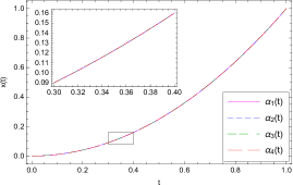
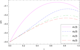
Figure 1: (Example 6.) Comparison between the approximate state (left) and control (right) functions obtained by Approach I with $M=5$ and different $\alpha(t)$ (40).

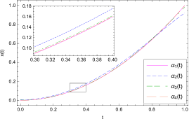
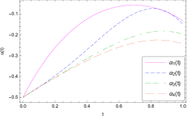
Figure 2: (Example 6.) Comparison between the approximate state (left) and control (right) functions obtained by Approach II with $M=5$ and different $\alpha(t)$ (40).

Table 2: (Example 6.) Numerical results for the performance index with $M=5$ and different $\alpha(t)$ (40).

Method	$\alpha_{1}(t)$	$\alpha_{2}(t)$	$\alpha_{3}(t)$	$\alpha_{4}(t)$
Approach I	$3.05\times{10}^{-33}$	$3.26\times{10}^{-33}$	$6.89\times{10}^{-33}$	$2.08\times{10}^{-33}$
Approach II	$2.74\times{10}^{-33}$	$1.56\times{10}^{-3}$	$1.71\times{10}^{-4}$	$2.50\times{10}^{-5}$

Consider now the following FOC-AP borrowed from Lotfi et al. (2013):

$$\min~{}J=\int_{0}^{1}\left[\left(x(t)-t^{\frac{5}{2}}\right)^{4}+(1+t^{2})\left(u(t)+t^{6}-\frac{15\sqrt{\pi}}{8}t\right)^{2}\right]dt$$ (41)

subject to

$${{}_{0}^{C}D}_{t}^{\frac{3}{2}}x(t)=tx^{2}(t)+u(t)$$ (42)

and the initial conditions $x(0)=x^{\prime}(0)=0$. For this problem, the state and control functions

$$x(t)=t^{\frac{5}{2}},\quad u(t)=-t^{6}+\frac{15\sqrt{\pi}}{8}t$$

minimize the performance index with the optimal value $J=0$. We have solved this problem by both approaches. The numerical results of applying Approach I to this problem, with different values of $M$, are presented in Figure 3 and Table 3. Figure 3 displays the approximate state (left) and control (right) functions obtained by $M=1,3,5,7$, together with the exact ones, while Table 3 reports the approximate values of the performance index. Here, we show that Approach II gives the exact solution by considering $M=1$. To do this, we suppose that

$${{}_{0}^{C}D}_{t}^{\frac{3}{2}}x(t)=A^{T}B(t)=a_{1}\left(t-\frac{1}{2}\right)+a_{0}$$

with

$$A=[a_{0},a_{1}]^{T}\text{ and }B(t)=\left[1,t-\frac{1}{2}\right]^{T}.$$

Therefore, we have

$$x(t)=A^{T}P_{t}^{\frac{3}{2}}B(t)=\frac{2}{3\sqrt{\pi}}(2a_{0}-a_{1})t^{\frac{3}{2}}+\frac{8}{15\sqrt{\pi}}a_{1}t^{\frac{5}{2}},$$ (43)

where

$$P_{t}^{\frac{3}{2}}=\left[\begin{array}[]{cc}\frac{4}{3\sqrt{\pi}}t^{\frac{3}{2}}&0\\ -\frac{2}{5\sqrt{\pi}}t^{\frac{3}{2}}&\frac{8}{15\sqrt{\pi}}t^{\frac{3}{2}}\\ \end{array}\right].$$

Using the dynamical control-affine system given by (42), we get

$$\begin{split}u(t)&=a_{1}\left(t-\frac{1}{2}\right)+a_{0}-t\left(\frac{2}{3\sqrt{\pi}}(2a_{0}-a_{1})t^{\frac{3}{2}}+\frac{8}{15\sqrt{\pi}}a_{1}t^{\frac{5}{2}}\right)^{2}\\ &=-\frac{64a_{1}^{2}}{225\pi}t^{6}+\left(\frac{32a_{1}^{2}}{45\pi}-\frac{64a_{0}a_{1}}{45\pi}\right)t^{5}+\left(\frac{16a_{0}a_{1}}{9\pi}-\frac{16a_{0}^{2}}{9\pi}-\frac{4a_{1}^{2}}{9\pi}\right)t^{4}+a_{1}t+a_{0}-\frac{a_{1}}{2}.\end{split}$$ (44)

By substituting (43) and (44) into (41), the value of the integral can be easily computed. Then, by taking into account the optimality condition, a system of nonlinear algebraic equations is obtained. Finally, by solving this system, we obtain

$$a_{0}=\frac{15\sqrt{\pi}}{16},\quad a_{1}=\frac{15\sqrt{\pi}}{8}.$$

By taking into account these values in (43) and (44), the exact optimal state and control functions are obtained. Lotfi et al. have solved this problem using an operational matrix technique based on the Legendre orthonormal functions combined with the Gauss quadrature rule. In their method, the approximate value of the minimum performance index with five basis functions has been reported as $7.82\times 10^{-9}$ while our suggested Approach II gives the exact value only with two basis functions.

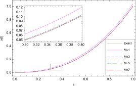
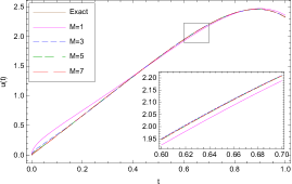
Figure 3: (Example 6.) Comparison between the exact and approximate state (left) and control (right) functions obtained by Approach I with different values of $M$.

Table 3: (Example 6.) Numerical results for the performance index obtained by Approach I with different $M$.

$M$	$1$	$3$	$5$	$7$
$J$	$5.24\times{10}^{-4}$	$7.59\times{10}^{-6}$	$4.65\times{10}^{-7}$	$5.86\times{10}^{-8}$

As we see, in this example, Approach II yields the exact solution with a small computational cost, while the precision of the results of Approach I increases by enlarging $M$. Note that here the optimal state function is not an infinitely smooth function.

As our last example, we consider the following FOC-AP Lotfi et al. (2013):

$$\min~{}J=\int_{0}^{1}\left[e^{t}\left(x(t)-t^{4}+t-1\right)^{2}+(1+t^{2})\left(u(t)+1-t+t^{4}-\frac{8000}{77\Gamma\left(\frac{1}{10}\right)}t^{\frac{21}{10}}\right)^{2}\right]dt$$

subject to

$${{}_{0}^{C}D}_{t}^{1.9}x(t)=x(t)+u(t),$$

$$x(0)=1,\quad x^{\prime}(0)=-1.$$

For this example, the following state and control functions minimize the performance index $J$ with minimum value $J=0$:

$$x(t)=t^{4}-t+1,\quad u(t)=-t^{4}+\frac{8000}{77\Gamma\left(\frac{1}{10}\right)}t^{\frac{21}{10}}+t-1.$$

This problem has been solved using the proposed methods with different values of $M$. By considering $M=1$, the numerical results of Approach I are shown in Figure 4. In this case, an approximation of the performance index is obtained as $J=7.21\times{10}^{-1}$. By choosing $M=2$, according to our numerical method, we have $n=2$. Therefore, we set

$$x{{}^{\prime\prime}}(t)=A^{T}B(t),$$

where

$$A=[a_{0},a_{1},a_{2}],\quad B(t)=\left[1,t-\frac{1}{2},t^{2}-t+\frac{1}{6}\right]^{T}.$$

Hence, using the initial conditions, the state function can be approximated by

$$x(t)=A^{T}P^{2}_{t}B(t)-t+1=\frac{a_{2}}{12}t^{4}+\frac{a_{1}-a_{2}}{6}t^{3}+\left(\frac{a_{0}}{2}-\frac{a_{1}}{4}+\frac{a_{2}}{12}\right)t^{2}-t+1,$$

where

$$P^{2}_{t}=\left[\begin{array}[]{ccc}\frac{t^{2}}{2}&0&0\\ -\frac{t^{2}}{6}&\frac{t^{2}}{6}&0\\ \frac{t^{2}}{36}&-\frac{t^{2}}{12}&\frac{t^{2}}{12}\\ \end{array}\right].$$

In the continuation of the method, we find an approximation of the control function $u$ using the control-affine dynamical system. Then, the method proceeds until solving the resulting system, which yields

$$a_{0}=4,\quad a_{1}=12,\quad a_{2}=12.$$

These values give us the exact solution of the problem. This problem has been solved in Lotfi et al. (2013) with five basis functions and the minimum value was obtained as $J=5.42\times 10^{-7}$ while our suggested Approach I gives the exact value with only three basis functions.

In the implementation of Approach II, we consider different values of $M$ and report the results in Table 4 and Figure 5. These results confirm that the numerical solutions converge to the exact one by increasing the value of $M$. Nevertheless, we see that since the exact state function $x$ is a smooth function, it takes much less computational effort to solve this problem by using Approach I.

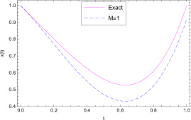
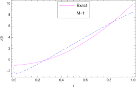
Figure 4: (Example 6.) Comparison between the exact and approximate state (left) and control (right) functions obtained by Approach I with $M=1$.

Table 4: (Example 6.) Numerical results for the performance index obtained by Approach II with different $M$.

$M$	$2$	$4$	$6$	$8$
$J$	$3.79\times{10}^{-4}$	$5.42\times{10}^{-7}$	$1.21\times{10}^{-8}$	$7.36\times{10}^{-10}$

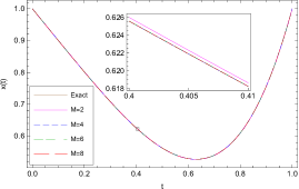
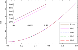
Figure 5: (Example 6.) Comparison between the exact and approximate state (left) and control (right) functions obtained by Approach II with different values of $M$.

7 Conclusions

Two numerical approaches have been proposed for solving variable-order fractional optimal control-affine problems. They use an accurate operational matrix of variable-order fractional integration for Bernoulli polynomials, to give approximations of the optimal state and control functions. These approximations, along with the Gauss–Legendre quadrature formula, are used to reduce the original problem to a system of algebraic equations. An approximation of the optimal performance index and an error bound were given. Some examples have been solved to illustrate the accuracy and applicability of the new techniques. From the numerical results of Examples 6 and 6, it can be seen that our Approach I leads to very high accuracy results with a small number of basis functions for optimal control problems in which the state function that minimizes the performance index is an infinitely smooth function. Moreover, from the results of Example 6, we conclude that Approach II may give much more accurate results than Approach I in the cases that the smoothness of ${{}_{0}^{C}D}_{t}^{\alpha(t)}x(t)$ is more than $x^{(n)}(t)$.

Conceptualization, Somayeh Nemati and Delfim F. M. Torres; Investigation, Somayeh Nemati and Delfim F. M. Torres; Software, Somayeh Nemati; Validation, Delfim F. M. Torres; Writing – original draft, Somayeh Nemati and Delfim F. M. Torres; Writing – review & editing, Somayeh Nemati and Delfim F. M. Torres.

Torres was funded by Fundação para a Ciência e a Tecnologia (FCT, the Portuguese Foundation for Science and Technology) through grant UIDB/04106/2020 (CIDMA).

References

• Machado et al. (2011) Machado, J.T.; Kiryakova, V.; Mainardi, F. Recent history of fractional calculus. Commun. Nonlinear Sci. Numer. Simul. 2011, 16, 1140–1153. doi:\changeurlcolorblack10.1016/j.cnsns.2010.05.027.
• Keshavarz et al. (2016) Keshavarz, E.; Ordokhani, Y.; Razzaghi, M. A numerical solution for fractional optimal control problems via Bernoulli polynomials. J. Vib. Control 2016, 22, 3889–3903. doi:\changeurlcolorblack10.1177/1077546314567181.
• Bhrawy et al. (2012) Bhrawy, A.H.; Tohidi, E.; Soleymani, F. A new Bernoulli matrix method for solving high-order linear and nonlinear Fredholm integro-differential equations with piecewise intervals. Appl. Math. Comput. 2012, 219, 482–497. doi:\changeurlcolorblack10.1016/j.amc.2012.06.020.
• Tohidi et al. (2013) Tohidi, E.; Bhrawy, A.H.; Erfani, K. A collocation method based on Bernoulli operational matrix for numerical solution of generalized pantograph equation. Appl. Math. Model. 2013, 37, 4283–4294. doi:\changeurlcolorblack10.1016/j.apm.2012.09.032.
• Toutounian and Tohidi (2013) Toutounian, F.; Tohidi, E. A new Bernoulli matrix method for solving second order linear partial differential equations with the convergence analysis. Appl. Math. Comput. 2013, 223, 298–310. doi:\changeurlcolorblack10.1016/j.amc.2013.07.094.
• Bazm (2015) Bazm, S. Bernoulli polynomials for the numerical solution of some classes of linear and nonlinear integral equations. J. Comput. Appl. Math. 2015, 275, 44–60. doi:\changeurlcolorblack10.1016/j.cam.2014.07.018.
• Sahu and Mallick (2019) Sahu, P.K.; Mallick, B. Approximate solution of fractional order Lane-Emden type differential equation by orthonormal Bernoulli’s polynomials. Int. J. Appl. Comput. Math. 2019, 5, Paper No. 89, 9. doi:\changeurlcolorblack10.1007/s40819-019-0677-0.
• Loh and Phang (2019) Loh, J.R.; Phang, C. Numerical solution of Fredholm fractional integro-differential equation with right-sided Caputo’s derivative using Bernoulli polynomials operational matrix of fractional derivative. Mediterr. J. Math. 2019, 16, Paper No. 28, 25. doi:\changeurlcolorblack10.1007/s00009-019-1300-7.
• Rosa and Torres (2018) Rosa, S.; Torres, D.F.M. Optimal control of a fractional order epidemic model with application to human respiratory syncytial virus infection. Chaos Solitons Fractals 2018, 117, 142–149. doi:\changeurlcolorblack10.1016/j.chaos.2018.10.021. arXiv:1810.06900
• Malinowska and Torres (2012) Malinowska, A.B.; Torres, D.F.M. Introduction to the fractional calculus of variations; Imperial College Press, London, 2012. doi:\changeurlcolorblack10.1142/p871.
• Malinowska et al. (2015) Malinowska, A.B.; Odzijewicz, T.; Torres, D.F.M. Advanced methods in the fractional calculus of variations; SpringerBriefs in Applied Sciences and Technology, Springer, Cham, 2015.
• Almeida et al. (2015) Almeida, R.; Pooseh, S.; Torres, D.F.M. Computational methods in the fractional calculus of variations; Imperial College Press, London, 2015. doi:\changeurlcolorblack10.1142/p991.
• Ali et al. (2019) Ali, M.S.; Shamsi, M.; Khosravian-Arab, H.; Torres, D.F.M.; Bozorgnia, F. A space-time pseudospectral discretization method for solving diffusion optimal control problems with two-sided fractional derivatives. J. Vib. Control 2019, 25, 1080–1095. doi:\changeurlcolorblack10.1177/1077546318811194. arXiv:1810.05876
• Nemati et al. (2019) Nemati, S.; Lima, P.M.; Torres, D.F.M. A numerical approach for solving fractional optimal control problems using modified hat functions. Commun. Nonlinear Sci. Numer. Simul. 2019, 78, 104849, 14. doi:\changeurlcolorblack10.1016/j.cnsns.2019.104849. arXiv:1905.06839
• Salati et al. (2019) Salati, A.B.; Shamsi, M.; Torres, D.F.M. Direct transcription methods based on fractional integral approximation formulas for solving nonlinear fractional optimal control problems. Commun. Nonlinear Sci. Numer. Simul. 2019, 67, 334–350. doi:\changeurlcolorblack10.1016/j.cnsns.2018.05.011. arXiv:1805.06537
• Rabiei et al. (2018) Rabiei, K.; Ordokhani, Y.; Babolian, E. Numerical solution of 1D and 2D fractional optimal control of system via Bernoulli polynomials. Int. J. Appl. Comput. Math. 2018, 4, Paper No. 7, 17. doi:\changeurlcolorblack10.1007/s40819-017-0435-0.
• Behroozifar and Habibi (2018) Behroozifar, M.; Habibi, N. A numerical approach for solving a class of fractional optimal control problems via operational matrix Bernoulli polynomials. J. Vib. Control 2018, 24, 2494–2511. doi:\changeurlcolorblack10.1177/1077546316688608.
• Rahimkhani and Ordokhani (2019) Rahimkhani, P.; Ordokhani, Y. Generalized fractional-order Bernoulli-Legendre functions: an effective tool for solving two-dimensional fractional optimal control problems. IMA J. Math. Control Inform. 2019, 36, 185–212. doi:\changeurlcolorblack10.1093/imamci/dnx041.
• Samko and Ross (1993) Samko, S.G.; Ross, B. Integration and differentiation to a variable fractional order. Integral Transform. Spec. Funct. 1993, 1, 277–300. doi:\changeurlcolorblack10.1080/10652469308819027.
• Lorenzo and Hartley (2002) Lorenzo, C.F.; Hartley, T.T. Variable order and distributed order fractional operators. Nonlinear Dyn. 2002, 29, 57–98. doi:\changeurlcolorblack10.1023/A:1016586905654.
• Abdeljawad et al. (2019) Abdeljawad, T.; Mert, R.; Torres, D.F.M. Variable order Mittag-Leffler fractional operators on isolated time scales and application to the calculus of variations. In Fractional derivatives with Mittag-Leffler kernel; Springer, Cham, 2019; Vol. 194, Stud. Syst. Decis. Control, pp. 35–47. arXiv:1809.02029
• Hassani and Naraghirad (2019) Hassani, H.; Naraghirad, E. A new computational method based on optimization scheme for solving variable-order time fractional Burgers’ equation. Math. Comput. Simulation 2019, 162, 1–17. doi:\changeurlcolorblack10.1016/j.matcom.2019.01.002.
• Odzijewicz et al. (2013) Odzijewicz, T.; Malinowska, A.B.; Torres, D.F.M. Fractional variational calculus of variable order. In Advances in harmonic analysis and operator theory; Birkhäuser/Springer Basel AG, Basel, 2013; Vol. 229, Oper. Theory Adv. Appl., pp. 291–301. doi:\changeurlcolorblack10.1007/978-3-0348-0516-2_16. arXiv:1110.4141
• Yan et al. (2019) Yan, R.; Han, M.; Ma, Q.; Ding, X. A spectral collocation method for nonlinear fractional initial value problems with a variable-order fractional derivative. Comput. Appl. Math. 2019, 38, Paper No. 66, 25. doi:\changeurlcolorblack10.1007/s40314-019-0835-3.
• Almeida et al. (2019) Almeida, R.; Tavares, D.; Torres, D.F.M. The variable-order fractional calculus of variations; SpringerBriefs in Applied Sciences and Technology, Springer, Cham, 2019. doi:\changeurlcolorblack10.1007/978-3-319-94006-9. arXiv:1805.00720
• Heydari and Avazzadeh (2018) Heydari, M.H.; Avazzadeh, Z. A new wavelet method for variable-order fractional optimal control problems. Asian J. Control 2018, 20, 1804–1817. doi:\changeurlcolorblack10.1002/asjc.1687.
• Mohammadi and Hassani (2019) Mohammadi, F.; Hassani, H. Numerical solution of two-dimensional variable-order fractional optimal control problem by generalized polynomial basis. J. Optim. Theory Appl. 2019, 180, 536–555. doi:\changeurlcolorblack10.1007/s10957-018-1389-z.
• Costabile et al. (2006) Costabile, F.; Dell’Accio, F.; Gualtieri, M.I. A new approach to Bernoulli polynomials. Rend. Mat. Appl. (7) 2006, 26, 1–12.
• Arfken (1966) Arfken, G. Mathematical methods for physicists; Academic Press, New York-London, 1966.
• Shen et al. (2011) Shen, J.; Tang, T.; Wang, L.L. Spectral methods; Vol. 41, Springer Series in Computational Mathematics, Springer, Heidelberg, 2011. doi:\changeurlcolorblack10.1007/978-3-540-71041-7.
• Canuto et al. (2006) Canuto, C.; Hussaini, M.Y.; Quarteroni, A.; Zang, T.A. Spectral methods; Scientific Computation, Springer-Verlag, Berlin, 2006.
• Lotfi et al. (2013) Lotfi, A.; Yousefi, S.A.; Dehghan, M. Numerical solution of a class of fractional optimal control problems via the Legendre orthonormal basis combined with the operational matrix and the Gauss quadrature rule. J. Comput. Appl. Math. 2013, 250, 143–160. doi:\changeurlcolorblack10.1016/j.cam.2013.03.003.