Longitudinal Coherence Enhancement of X-Ray Free Electron Lasers

Abstract

We present a new scheme for establishing longitudinal coherence in the output of X-ray FELs. It uses a sequence of undulators and delay chicanes and the careful tailoring of the initial e-beam with time dependent focusing. Simulation of a simplified model of the FEL shows that the idea works well.

1 Introduction

Though the new generation of X-ray free electron lasers (FELs) produces X-rays that are almost completely coherent transversally, longitudinally the output is ‘spiky’, as indicated roughly in figure 1; i.e. the spectral bandwith is larger than desired, [1].

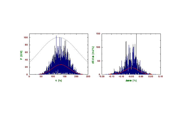
Figure 1: Typical longitudinal output of an X-ray FEL.

Schemes have been proposed to deal with this problem such as the Geloni idea, [3], [2], and echo enhanced harmonic generation to produce seeds in the soft X-ray regime, [6], [4]. In this paper we will outline a new approach to this problem that might extrapolate more easily to shorter wavelengths and be more easily tunable.

In the next section we discuss the basic idea of our approach, noting that a set of undulators and e-beam chicanes combined with initially longitudinally decreasing wave intensity might be used to increase coherence lengths. In section $3$ we show that an initial photon beam with decreasing intensity can be created by tailored electron beam size variations. In section $4$ we present simulations of a reduced model of the X-ray FEL that indicate that our idea seems to work well. In the final section we discuss our results and point out further work with more realistic models that is required. In appendix A we present the Maxima code used in the simulations. In appendix B we discuss a simple example of how to create the tailored e-beam size.

2 Basic Idea

Typically a spike covers a coherence length and is longitudinally coherent over it; similarly the other spikes are about a coherence length in duration and are longitudinally coherent but are not in phase with the other spikes. One approach might be to delay the electron beam by using a chicane consisting of dipoles to increase the electron travel distance by a coherence length during the chicane. The photon bunch then travels forward in the electron bunch by a coherence length (i.e. the electrons fall behind by a coherence length), leaving electrons nearer the tail bunched in phase with the photons now one slice ahead but with very few photons. In the next section of undulator the electron oscillations toward the tail of the bunch rapidly grow at the same phase as the now forward photons since the electrons are strongly seeded. Of course, this won’t increase the coherence length of the photons completely because the photons that are moved forward in the electron bunch will interfere with the phase of the electrons in the forward section and tend to cancel the field. To overcome this cancellation we need to add one more idea.

(Note that a chicane consisting of a positive dipole followed by a negative dipole is probably adequate, though a combination of a half positive dipole, followed by a full negative dipole followed by a half positive dipole probably is more achromatic and has smaller higher order terms.)

Suppose instead that the laser intensity, after a few growth times, decreases along the bunch, being stronger toward the rear and weaker toward the front, as shown in figure 2.

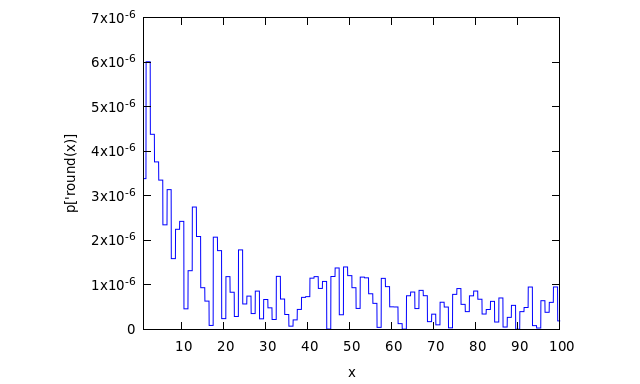
Figure 2: Initial decreasing longitudinal power with bunch length of an X-ray FEL.

In this case, when the photon spike moves forward it encounters electrons with less bunching at the wrong phase and can convert the electron bunching to the right phase. After a few growth lengths, the coherence length toward the tail is longer. Repeating this process, the next time we slide the photons forward we need to go through fewer growth lengths because of the larger amplitudes. After a few repetitions of this process, essentially the entire photon bunch should be longitudinally coherent.

3 Decreasing Longitudinal Intensity

Of course we have to show how to achieve the temporal output shown in figure 2. To do this we refer to the growth formulae of [5], [1]. The FEL power at a point $z$ down the undulator is given by

$$P=P_{0}e^{z/L_{G}},$$ (1)

where $P_{0}$ is the initial power and $L_{G}$ is the growth length. The growth length is given by

$$L_{G}={\Lambda_{u}\over 4\pi\sqrt{3}\rho},$$ (2)

where $\Lambda_{u}$ is the undulator period and $\rho$ is the Pierce parameter given by

$$\rho=\left[{1\over 16}{I_{e}\over I_{A}}{K_{0}^{2}\left[JJ\right]^{2}\over\gamma_{0}^{3}\sigma_{x}^{2}k_{u}^{2}}\right]^{1\over 3},$$ (3)

with $I_{e}$ the beam current, $I_{A}$ the Alfven current, $K_{0}$ the undulator parameter, $k_{u}$ is the undulator wave number, $\gamma_{0}$ is the relativistic e-beam factor, $\left[JJ\right]=J_{0}(\xi)-J_{1}(\xi)$, (Bessel functions), with $\xi=K_{0}^{2}/(4+2K_{0}^{2})$ (planar wiggler), and $\sigma_{x}$ is the RMS transverse beam size. Note the dependence on beam size, $\sigma_{x}$. We can rewrite the growth length as

$$L_{G}=\chi\sigma_{x}^{2/3},$$ (4)

where $\chi$ contains all the remaining factors of $L_{G}$. If we consider two slices of the electron bunch and assume that they have transverse sizes $\sigma_{x1}$ and $\sigma_{x2}$, then, after $N_{G}$ growth lengths, the relative power in each slice (assuming equal initial amplitudes) will satisfy

$${P_{2}\over P_{1}}=\exp(N_{G}({\sigma_{x1}^{2/3}\over\sigma_{x2}^{2/3}}-1))$$ (5)

If we take $\sigma_{x2}=2\sigma_{x1}$, i.e. the forward electrons larger transversally than the trailing electrons, then

$${P_{2}\over P_{1}}=\exp(-0.37N_{G}),$$ (6)

and after three growth lengths the power should look something like figure 2. Thus, we need to show how to achieve a transverse beam profile that looks roughly like figure 3.

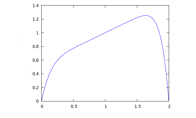
Figure 3: Rough indication of the beam radius needed for the correct variable gain.

To achieve such a beam shape requires transverse forces that vary from the front to the back of the bunch, i.e. time-dependent forces. We thus need time dependent electromagnetic fields that vary on such a rapid time scale. We give an example of a scheme to do this in appendix B.

4 Simulations

To investigate the efficiency of this scheme we have performed a number of simulations of a reduced model of the FEL with these elements.

We divide the electron beam into a number of slices, each uniformly about a coherence length in size and divide the photon beam into a equal number of longitudinal slices. The coherence length, $L_{c}$, is given by

$$L_{c}={\lambda\over 4\pi\rho},$$ (7)

where $\lambda$ is the XFEL wavelength, and $\rho$ is the Pierce parameter defined earlier. In addition, the electron beam and photon beam are divided into a number of phases (typically $24$) of the electron waves and photon waves equally spaced around $360$ degrees.

4.1 Initialization

Initially, the electron beam and photon beam are seeded with small random amplitudes for each slice and each phase. For each slice, we then randomly choose one phase and make the amplitude for the electron beam and photon beam for that phase $4$ times larger. In other words we assume we have already gone through one section of undulator and that SASE has produced the typical spiky output at low power. The resultant initial beam for one case is shown in figure 4

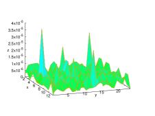
Figure 4: Initial photon beam for one run.

As can be seen, this initial beam is not coherent.

4.2 Time advance

Once we initialize the beams (electron and photon) we send the beams through a number of sections where they interact. A section consists of two parts: 1) an undulator section where the electrons drive the photons and the photons drive the electrons, and 2) a delay chicane where the electrons slide back by a slice, i.e. the photons slide forward by one slice. We thus describe the electrons as an array, $e(n,i,j)$ where $n$ labels the time step, $i$ labels the longitudinal slice number, and $j$ labels the phase number. Likewise, the photons are described as an array $p(n,i,j)$ where $n$ labels the time step, $i$ labels the longitudinal slice number, and $j$ labels the phase number. These arrays for $n=1$ (initial time) are shown in figure 4 for one case. The undulator part of the advance satisfies the equations

$$e(n+1,i,j)=e(n,i,j)+\Gamma(i)p(n,i,j)$$ (8)

$$p(n+1,i,j)=p(n,i,j)+\Gamma(i)e(n,i,j)$$ (9)

where $\Gamma(i)$ is a growth that varies along the longitudinal slices, $i$. Note that $\Gamma$ does not depend on the phase; all phases are assumed to have the same growth rates.

In the chicane part of the advance the photons slip forward by one slice relative to the electrons while the electrons are unchanged (i.e. slip backward relative to the photons). Of course the slice of photons in the very front is simply lost to the simulation (no longer followed), and a new slice of photons with very small random amplitudes for each slice and phase is injected at the rear. The Maxima code that performs these advances is shown in appendix A.

Of course, in the simulation the growth factor $\Gamma(i)$ must be specified. For a more realistic simulation this would be found by following the e-beam properties and using the growth formula. In these simulations we simply specify the growth function assuming that it comes from an e-beam with radius that increases toward the front.

4.3 Simulation results

Starting with the initial beams of figure 4 we first tried a simulation with chicanes inserted but with a constant growth rate for all phases and all slices, i.e. no beam size variation. The results at three times are shown in figure 5.

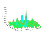
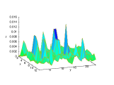
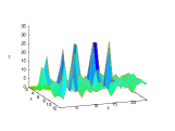
Figure 5: For the case with no beam size variation the initial photons (left), after 4 steps (middle), and after 9 steps (right).

As can be seen there is almost no improvement in the longitudinal coherence. In a simulation in which the growth rate decreases with the slice number reflecting an increasing e-beam size toward the front the results are shown in figure 6

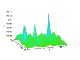
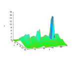
Figure 6: For a case with beam size variation the initial photons (left), after 4 steps (middle), and after 9 steps (right).

There is significant improvement in the longitudinal coherence. Also, recall that what is shown are amplitudes; the energies are proportional to the square of the amplitudes so the energy is almost completely in one phase of the photons. If we plot the square of the final results of figure 6 we get figure 7

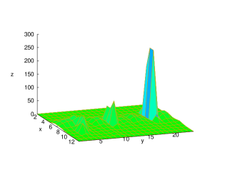
Figure 7: photon beam energy at the final time

The concentration on a single phase is evident. Different values of the constants in the simulation lead to qualitatively similar results, differing only in the number of steps required to establish a dominant phase.

5 Discussion

We have presented a new scheme for establishing longitudinal coherence in the output of X-ray FELs. It requires a sequence of undulators and delay chicanes and the careful tailoring of the initial e-beam with time dependent focusing. Simulation of a simplified model of the FEL showed that the idea works extremely well.

Of course, a completely convincing demonstration of this idea would require more realistic and fully self consistent simulations that would establish a realistic set of parameters to achieve coherence and determine the practicality of this scheme.

6 Appendix A

In this appendix we present the Maxima simulation code used in this paper. The values of the constants are representative and were varied in different runs.

kill(all);
/* # We begin initializing the random number generator. */
/* # Just change nrand for different randoms. */
nrand:17;
for i:1 thru nrand do
junk:random(1.0);
end;

/* #The number of growth sections is nsteps. */
nsteps:9;
/* # The number of slices in the e-beam and photon beam is nslice. */
nslice:12;
/* # The number of mode phases is nphase. */
nphase:24;

array(tx,nphase);
array(ty,nslice);
array(tstep,nsteps+1);
for i:1 thru nphase do tx[i]:i;
for i:1 thru nslice do ty[i]:i;
for i:1 thru nsteps+1 do tstep[i]:i;

array(p,nsteps+1,nslice,nphase);
array(e,nsteps+1,nslice,nphase);
/* # We initialize the amplitudes of the e-beam phases with small values. */
/* # The first index of e is the step number (starting at 1). */
/* # The second index of e is the slice number. */
/* # The third index of e is the phase number. */
for i:1 thru nslice do
(for j:1 thru nphase do
e[1,i,j]:0.00001*random(1.0));

/* /“* # We initialize the amplitudes of the photon beam phases with small values. *“/ */
/* /“* # The first index of p is the step number (starting at 1). *“/ */
/* /“* # The second index of p is the slice number. *“/ */
/* /“* # The third index of p is the phase number. *“/ */
for i:1 thru nslice do block(
for j:1 thru nphase do
p[1,i,j]:0.00001*random(1.0));

/* For each slice we find the max of the random values *?
/* and multiply it by a factor. */

for i:1 thru nslice do block(
temp[i]:0.0,
for j:1 thru nphase do block(
if e[1,i,j] ¿ temp[i] then temp[i]:e[1,i,j]));

for i:1 thru nslice do block(
for j:1 thru nphase do block(
if e[1,i,j] = temp[i] then
block(e[1,i,j]:4.0*e[1,i,j],p[1,i,j]:4.0*p[1,i,j])));

/* # We take the basic growth to be gamma0, giving growth */
/* # of gamma0^2 in a section. */
gamma0:3.9;

/* Choosing alpha=0.5 gives decreasing growth toward the front. */
/* Choosing alpha=0 gives constant growth from front to back. */
alpha:0.5;
/* alpha:0.0; */
array(slicegrowth,nslice);
/* # We make the growth (slicegrowth) of each slice and each growth step to */
/* # be less than gamma0 depnding on the slice number and step number. */

for j:1 thru nslice do
slicegrowth[j]:gamma0*(1-alpha*(j-1)/(nslice));

/* # Each growth step consists of an exponential growth of */
/* # e and p (for all phases) followed by a transfer forward */
/* # of the photon beam (renumbering indices) with a new */
/* # slice of photons injected with a small random value */
/* # for all phases. */
for n:1 thru nsteps do block(
/* # First the growth part. */
for i:1 thru nslice do block(
for j:1 thru nphase do block(
e[n+1,i,j]:e[n,i,j]+slicegrowth[i]*p[n,i,j],
p[n+1,i,j]:p[n,i,j]+slicegrowth[i]*e[n,i,j])),
/* # Store values in a temporary array. */

for i:1 thru nslice do block(
for j:1 thru nphase do block(
ptemp[i,j]:p[n+1,i,j])),
/* # Slide the photons forward. */
for i:2 thru nslice do block(
for j:1 thru nphase do block(
p[n+1,i,j]:ptemp[i-1,j])),

for j:1 thru nphase do
p[n+1,1,j]:0.2*p[n+1,1,j]
);

g(i,x,y):=block(x1:round(x),y1:round(y),p[i,x1,y1])$
set˙plot˙option([elevation,70]);
set˙plot˙option([azimuth,70]);
set˙plot˙option([legend,false]);

for istep:1 thru nsteps+1 do
plot3d(g(istep,x,y),[x,1,nslice],[y,1,nphase],
[grid,nslice,nphase],[gnuplot˙term,ps],
[gnuplot˙out˙file,concat(”sharp”,istep,”.eps”)]);

kill(g,x1,y1);
g(i,x,y):=block(x1:round(x),y1:round(y),p[i,x1,y1]^2)$
set˙plot˙option([elevation,70]);
set˙plot˙option([azimuth,70]);
set˙plot˙option([legend,false]);

for istep:1 thru nsteps+1 do
plot3d(g(istep,x,y),[x,1,nslice],[y,1,nphase],
[grid,nslice,nphase],[gnuplot˙term,ps],
[gnuplot˙out˙file,concat(”sharpsq”,istep,”.eps”)]);

7 Appendix B

To achieve such a beam shape requires transverse forces that vary from the front to the back of the bunch, i.e. time-dependent forces. We thus need time dependent electromagnetic fields that vary on such a rapid time scale. These forces have to have a wavelength about four times the bunch length. For a $20\mu$m bunch we thus need a wavelength of about $100\mu$m, possibly a laser. The laser needs to be injected in a structure (possibly a grating) to make use of the transverse focusing fields (vacuum fields produce no net focussing). Note that the transverse size of the beam should also be a significant fraction of the wavelength to make efficient use of the field, though not so large that nonlinearities become important.

If we assume such forces act over a small distance causing a change in transverse angle of $\Delta\theta$ and are followed by a drift of length $L$, then the transverse size change (we assume cylindrical symmetry for simplicity) is given by

$$\Delta r=L\Delta\theta,$$ (10)

where $\Delta\theta$ and thus $\Delta r$ will vary from particle to particle, depending on the forces. Now

$$\Delta\theta={\Delta p\over p},$$ (11)

where $p$ is the momentum and the change in momentum caused by the defocusing forces is

$$\Delta p=eB\Delta t,$$ (12)

with $B$ the magnetic defocusing field, $e$ the charge, and $\Delta t$ the time over which the force acts. If we assume a set of $N_{c}$ small cavities, each of length $\Lambda/2$, then

$$\Delta t={N_{c}\Lambda\over 2c},$$ (13)

and the angle change is

$$\Delta\theta\approx{eBN_{c}\Lambda\over 4pc},$$ (14)

where an extra factor of $1/2$ is an approximation of the transit time factor. Of course, for relativistic particles, $pc\approx{\cal E}$, where ${\cal E}$ is the particle energy. Thus, requiring $\Delta r=r_{B}$ for some particles gives the requirement

$${eBN_{c}\Lambda\over 4{\cal E}}\approx{r_{B}\over L}.$$ (15)

If we assume the field extends out to $\approx\Lambda$, then the field at the beam edge is

$$B\approx{r_{B}B_{max}\over\Lambda}.$$ (16)

Plugging this into equation 15 we get

$${eB_{max}N_{c}\over 4{\cal E}}\approx{1\over L}.$$ (17)

As an example, if we take

$${\cal E}= 12\,{\rm GeV},$$ (18)

$$N_{c}= 10\,,$$ (19)

$$L= 5\,{\rm m},$$ (20)

then we find

$$B_{max}\approx 3.3\,{\rm Tesla},$$ (21)

a reasonable value at $3.2$ THz.

References

- [1] W.A. Barletta, J. Bisognano, J.N. Corlett, P. Emma, Z. Huang, K.-J. Kim, R. Lindberg, J.B. Murphy, G.R. Neil, D.C. Nguyen, C. Pellegrini, R.A. Rimmer, F. Sannibale, G. Stupakov, R.P. Walker, A.A. Zholents, Nuclear Instruments and Methods in Physics Research A 618 (2010) 69–96.
- [2] P. Emma, IPAC 2012.
- [3] G. Geloni, V. Kocharyan, E. Saldin, DESY 10-133, Aug. 2010.
- [4] E. Hemsing et al. Echo-enabled harmonics up to the 75th order from precisely tailored electron beams, Nature Photonics (2016). DOI: 10.1038/nphoton.2016.101
- [5] Z. Huang and K. Kim, PRSTAB 10 034801, (2007).
- [6] Dao Xiang and Gennady Stupakov, Echo-enabled harmonic generation free electron laser, PHYSICAL REVIEW SPECIAL TOPICS - ACCELERATORS AND BEAMS 12, 030702 (2009)