Intrinsic Probing through Dimension Selection

Abstract

Most modern NLP systems make use of pre-trained contextual representations that attain astonishingly high performance on a variety of tasks. Such high performance should not be possible unless some form of linguistic structure inheres in these representations, and a wealth of research has sprung up on probing for it. In this paper, we draw a distinction between intrinsic probing, which examines how linguistic information is structured within a representation, and the extrinsic probing popular in prior work, which only argues for the presence of such information by showing that it can be successfully extracted. To enable intrinsic probing, we propose a novel framework based on a decomposable multivariate Gaussian probe that allows us to determine whether the linguistic information in word embeddings is dispersed or focal. We then probe fastText and BERT for various morphosyntactic attributes across 36 languages. We find that most attributes are reliably encoded by only a few neurons, with fastText concentrating its linguistic structure more than BERT.

1 Introduction

Natural language processing (NLP) is enamored of contextual word representations—and for good reason! Contextual word-embedders, e.g. BERT Devlin et al. (2019) and ELMo Peters et al. (2018), have bolstered NLP model performance on myriad tasks, such as syntactic parsing (Kitaev et al., 2019), coreference resolution (Joshi et al., 2019), morphological tagging (Kondratyuk, 2019) and text generation (Zellers et al., 2019). Given the large empirical gains observed when they are employed, it is all but certain that word representations derived from neural networks encode some continuous analogue of linguistic structures.author=lucas,color=blue!10,size=,fancyline,caption=,]Took off the next sentence, it was redundant

Exactly what these representations encode about linguistic structure, however, remains little understood. Researchers have studied this question by attributing function to specific network cells with visualization methods (Karpathy et al., 2015; Li et al., 2016) and by probing (Alain and Bengio, 2017; Belinkov and Glass, 2019), which seeks to extract structure from the representations. Recent work has probed various representations for correlates of morphological Belinkov et al. (2017); Giulianelli et al. (2018), syntactic Hupkes et al. (2018); Zhang and Bowman (2018); Hewitt and Manning (2019); Lin et al. (2019), and semantic Kim et al. (2019) structure.

Figure 1: Scatter plot of the two most informative BERT dimensions for English present and past tense. The contours belong to our probe.

Most current probing efforts focus on what we term extrinsic probing, where the goal is to determine whether the posited linguistic structure is predictable from the learned representation. Generally, extrinsic probing works argue for the presence of linguistic structure by showing that it is extractable from the representations using a machine learning model. In contrast, we focus on intrinsic probing—whose goals are a proper superset of the goals of extrinsic probing. In intrinsic probing, one seeks to determine not only whether a signature of linguistic structure can be found, but also how it is encoded in the representations. In short, we aim to discover which particular “neurons” (a.k.a.  dimensions) in the representations correlate with a given linguistic structure.author=ryan,color=violet!40,size=,fancyline,caption=,]Hang!author=lucas,color=blue!10,size=,fancyline,caption=,]Which sentence does this refer to? Also, Hang == delete? Intrinsic probing also has ancillary benefits that extrinsic probing lacks; it can facilitate manual analyses of representations and potentially yield a nuanced view about the information encoded by them.

The technical portion of our paper focuses on developing a novel framework for intrinsic probing: we scan sets of dimensions, or neurons, in a word vector representation which activate when they correlate with target linguistic properties. We show that when intrinsically probing high-dimensional representations, the present probing paradigm author=ryan,color=violet!40,size=,fancyline,caption=,]What is the present paradigm? I am confused.author=lucas,color=blue!10,size=,fancyline,caption=,]better? is insufficient (§ 2). Current probes are too slow to be used under our framework, which invariably leads to low-resolution scans that can only look at one or a few neurons at a time.author=ryan,color=violet!40,size=,fancyline,caption=,]The logical structure of the previous two paragraphs isn’t tight enough for my liking.author=lucas,color=blue!10,size=,fancyline,caption=,]Is this better? Instead, we introduce decomposable probes, which can be trained once on the whole representation and henceforth be used to scan any selection of neurons. To that end, we describe one such probe that leverages the multivariate Gaussian distribution’s inherent decomposability, and evaluate its performance on a large-scale, multi-lingual, morphosyntactic probing task (§ 3).

We experiment on 36 languages from the Universal Dependencies treebanks (Nivre et al., 2017). We find that all the morphosyntactic features we considered are encoded by a relatively small selection of neurons. In some cases, very few neurons are needed; for instance, for multilingual BERT English representations, we see that, with two neurons, we can largely separate past and present tense in Fig. 1. In this, our work is closest to Lakretz et al. (2019), except that we extend the investigation beyond individual neurons—a move which is only made tractable by decomposable probing. We also provide analyses on morphological features beyond number and tense. Across all languages, 35 out of 768 neurons on average suffice to reach a reasonable amount of encoded information, and adding more yields diminishing returns (see Fig. 2). Interestingly, in our head-to-head comparison of BERT and fastText, we find that fastText almost always encodes information about morphosyntactic properties using fewer dimensions.

2 Probing through Dimension Selection

The goal of intrinsic probing is to reveal how “knowledge” of a target linguistic property is structured within a neural network-derived representation. If said property can be predicted from the representations, we expect that this is because the neural network encodes this property (Giulianelli et al., 2018).author=ryan,color=violet!40,size=,fancyline,caption=,]We should get rid of the bigram “demonstrates knowledge”. I would prefer “predictable from” or something that is closer to what we actually doauthor=lucas,color=blue!10,size=,fancyline,caption=,]better? We can then determine whether a probe requires a large subset or a small subset of dimensions to predict the target property reliably. Particularly small subsets could be used to manually analyze a network and its decision process, and potentially reveal something about how specific neural architectures learn to encode linguistic information.

To formally describe our framework, we first define the necessary notation. We consider the probing of a word representation ${\boldsymbol{h}}\in\mathbb{R}^{d}$ for morphosyntax. In this work, our goal is find a subset of dimensions $C\subseteq D=\{1,\ldots,d\}$ such that the corresponding subvector of ${\boldsymbol{h}}_{C}$ contains only the dimensions that are necessary to predict the target morphosyntactic property we are probing for. For all possible subsets of dimensions $C\subseteq D$, and some random variable $\Pi$ that ranges over $P$ property values $\{\pi_{1},\ldots,\pi_{P}\}$, we consider a general probabilistic probe: $p_{{\boldsymbol{\theta}}_{C}}(\Pi=\pi\mid{\boldsymbol{h}}_{C})$; note that the model is conditioned on ${\boldsymbol{h}}_{C}$, not on ${\boldsymbol{h}}$. Our goal is to select a subset of dimensions using the log-likelihood of held-out data. We term this type of probing dimension selection. One can express dimension selection as the following combinatorial optimization problem:

$$C^{\star}=\operatorname*{argmax}_{\begin{subarray}{c}C\subseteq D,\\ |C|\leq k\end{subarray}}\sum_{n=1}^{N}\log p_{{\boldsymbol{\theta}}_{C}}(\pi^{(n)}\mid{\boldsymbol{h}}^{(n)}_{C})$$ (1)

where $\{({\boldsymbol{h}}_{C}^{(n)},\pi^{(n)})\}_{n=1}^{N}$ is a held-out dataset. Importantly, for complicated models we will require a different parameter set ${\boldsymbol{\theta}}_{C}$ for each subset $C\subseteq D$. In the general case, solving a subset selection problem such as eq. 1 is NP-Hard (Binshtok et al., 2007). Indeed, without knowing more about the structure of $p_{{\boldsymbol{\theta}}_{C}}$ we would have to rely on enumeration to solve this problem exactly. As there are ${d\choose k}$ possible subsets, it takes a prohibitively long time to enumerate them all for even small $d$ and $k$.

Greed is not Enough.

A natural first approach to approximate a solution to eq. 1 is a greedy algorithm (Kleinberg and Tardos, 2005, Chapter 4). Such an algorithm chooses the dimension that results in the largest increase to the objective at every iteration. However, some probes, such as neural network probes, need to be trained with a gradient-based method for many epochs. In such a case, even a greedy approximation is prohibitively expensive. For example, to select the first dimension, we train $d$ probes and take the best. To select the second dimension, we train $d-1$ probes and take the best. This requires training $\mathcal{O}(dk)$ networks! In the case of BERT, we have $d=768$ and we would generally like to consider $k$ at least up to $50$. Training on the order of $38400$ neural models to probe for just one morphosyntactic property is generally not practical. What we require is a decomposable probe, which can be trained once on all dimensions and then be used to evaluate the log-likelihood of any subset of dimensions in constant or near-constant time. To the best of our knowledge, no probes in the literature exhibit this property; the primary technical contribution of the paper is the development of such a probe in § 3.

Other Selection Criteria.

Our exposition above uses the log-likelihood of held-out data as a selection criterion for a subset of dimensions; however, any function that scores a subset of dimensions is suitable. For example, much of the current probing literature relies on accuracy to evaluate probes (Conneau et al., 2018; Liu et al., 2019, inter alia), and two recent papers motivate a probabilistic evaluation with information theory (Pimentel et al., 2020b; Voita and Titov, 2020). One could select based on accuracy, mutual information, or anything else within our framework. In fact, recent work in intrinsic probing by Dalvi et al. (2019) could be recast into our framework if we chose a dimension selection criterion based on the magnitude of the weights of a linear probe. However, we suspect that a performance-based dimension selection criterion (e.g., log-likelihood) should be more robust given that a weight-based approach is sensitive to feature collinearity, variance and regularization. As we mentioned before, performance-based selection requires a probe to be decomposable, and to the best of our knowledge, this is not the case for the the linear probe of Dalvi et al. (2019). author=ryan,color=violet!40,size=,fancyline,caption=,]This last sentence does not make sense to me!author=lucas,color=blue!10,size=,fancyline,caption=,]better?

3 A Decomposable Probe for Morphosyntactic Properties

Using the framework introduced above, our goal is to probe for morphosyntactic properties in word representations. We first describe the multivariate Gaussian distribution as it is responsible for our probe’s decomposability (§ 3.1), and provide some more notation (§ 3.2). We then describe our model (§ 3.3) and a Bayesian formulation (§ 3.4).

3.1 Properties of the Gaussian

The multivariate Gaussian distribution is defined as author=lucas,color=blue!10,size=,fancyline,caption=,]check definition in http://www.inf.ed.ac.uk/teaching/courses/mlpr/2017/notes/w7c_gaussian_processes.html

$$\mathcal{N} (\mathbf{x}\mid{\boldsymbol{\mu}},\Sigma)=$$ (2)

$$|2\pi\Sigma|^{-\frac{1}{2}}\exp\left({-\frac{1}{2}(\mathbf{x}-{\boldsymbol{\mu}})^{\top}\Sigma^{-1}(\mathbf{x}-{\boldsymbol{\mu}})}\right)$$

where ${\boldsymbol{\mu}}$ is the mean of the distribution and $\Sigma$ is the covariance matrix. We review the multivariate Gaussian with emphasis on the properties that make it ideal for intrinsic morphosyntactic probing.

Firstly, it is decomposable. Given a multivariate Gaussian distribution over $\mathbf{x}=[\mathbf{x}_{1}\,\,\mathbf{x}_{2}]^{\top}$ author=lucas,color=blue!10,size=,fancyline,caption=,]check definition in http://www.inf.ed.ac.uk/teaching/courses/mlpr/2017/notes/w7c_gaussian_processes.html

$$p(\mathbf{x}) =\mathcal{N}(\mathbf{x}\mid{\boldsymbol{\mu}},\Sigma)=$$ (3)

$$\mathcal{N}\left(\begin{bmatrix}\mathbf{x}_{1}\\ \mathbf{x}_{2}\end{bmatrix}\mathrel{\Big{|}}\begin{bmatrix}{\boldsymbol{\mu}}_{1}\\ {\boldsymbol{\mu}}_{2}\end{bmatrix},\begin{bmatrix}\Sigma_{11}&\Sigma_{12}\\ \Sigma_{12}^{\top}&\Sigma_{22}\end{bmatrix}\right)$$

the marginals for $\mathbf{x}_{1}$ and $\mathbf{x}_{2}$ may be computed as author=lucas,color=blue!10,size=,fancyline,caption=,]Murphy 4.68

$$p(\mathbf{x}_{1}) =\mathcal{N}(\mathbf{x}_{1}\mid{\boldsymbol{\mu}}_{1},\Sigma_{11})$$ (4)

$$p(\mathbf{x}_{2}) =\mathcal{N}(\mathbf{x}_{2}\mid{\boldsymbol{\mu}}_{2},\Sigma_{22})$$ (5)

This means that if we know ${\boldsymbol{\mu}}$ and $\Sigma$, we can obtain the parameters for any subset of dimensions of $\mathbf{x}$ by selecting the appropriate subvector (and submatrix) of ${\boldsymbol{\mu}}$ ($\Sigma$). As we will see in § 3.3, this property is the very centerpiece of our probe. Secondly, the Gaussian distribution is the maximum entropy distribution over the reals given a finite mean and covariance and no further information. Thus, barring additional information, the Gaussian is a good default choice. Jaynes (2003, Chapter 7) famously argued in favor of the Gaussian because it is the real-valued distribution with support $(-\infty,\infty)$ that makes the fewest assumptions about the data (beyond its first two moments).

3.2 Notation for Morphosyntactic Probing

author=lucas,color=blue!10,size=,fancyline,caption=,inline,]I reworked our explanation of the notation. Most importantly, I axed the sentence notation. Also added footnote and changed indexing.

We now provide some notation for our morphosyntactic probe. Let $\{{\boldsymbol{h}}^{(1)},\ldots,{\boldsymbol{h}}^{(N)}\}$ be word representation vectors in $\mathbb{R}^{d}$ for $N$ words $\{w^{(1)},\ldots,w^{(N)}\}$ from a corpus. For example, these could be embeddings output by fastText (Bojanowski et al., 2017), or contextual representations according to ELMo (Peters et al., 2018) or BERT (Devlin et al., 2019). Furthermore, let $\{\mathbf{m}^{(1)},\ldots,\mathbf{m}^{(N)}\}$ be the morphosyntactic tags associated with each of those words in the sentential context in which they were found.

Let $\mathcal{A}=\{a_{1},\ldots,a_{|\mathcal{A}|}\}$ be a universalauthor=ryan,color=violet!40,size=,fancyline,caption=,]Cite the UniMorph paper hereauthor=lucas,color=blue!10,size=,fancyline,caption=,]added it to footnote, is this what you meant? or do you want it in the main text? set of morphosyntactic attributes in a language, e.g. person, tense, number, etc. For each attribute $a\in\mathcal{A}$, let ${\mathcal{V}}_{a}$ be that attribute’s universal set of possible values. For instance, we have $\mathcal{V}_{\textsc{person}}=\{1,2,3\}$ for most languages. For this task, we will further decompose each morphosyntactic tag as a set of attribute–value pairs $\mathbf{m}^{(i)}=\langle a_{1}\!=\!v_{1},\ldots,a_{|\mathbf{m}^{(i)}|}\!=\!v_{|\mathbf{m}^{(i)}|}\rangle$ where each attribute $a_{j}$ is taken from the universal set of attributes $\mathcal{A}$, and each value $v_{j}$ is taken from a set $\mathcal{V}_{a_{j}}$ of universal values specific to that attribute. For example, the morphosyntactic tag $\mathbf{m}$ for the English verb “has” would be $\{\textsc{person}=3,\textsc{number}=\textsc{sg},\textsc{tense}=\textsc{prs}\}$.

3.3 Our Decomposable Generative Probe

We now present our decomposable probabilistic probe. We model the joint distribution between embeddings and a specific attribute’s values

$$p({\boldsymbol{h}},v)=p({\boldsymbol{h}}\mid v)\,p(v)$$ (6)

where we define

$$p({\boldsymbol{h}}\mid v)=\mathcal{N}({\boldsymbol{h}}\mid{\boldsymbol{\mu}}_{v},\Sigma_{v})$$ (7)

where ${\boldsymbol{\mu}}_{v}$ and $\Sigma_{v}$ are the value-specific mean and covariance. We further define

$$p(v)=\mathrm{Categorical}\left(\mathcal{V}_{a}\right)$$ (8)

This allows each value to have a different probability of occurring. This is important since our probe should be able to model that, e.g.  the 3rd person is more prevalent than the 1st person in corpora derived from Wikipedia. author=ryan,color=violet!40,size=,fancyline,caption=,]There must be a cleaner way to say this. Like, the Categorical has $|\mathcal{V}_{a}|-1$ free parameters?author=lucas,color=blue!10,size=,fancyline,caption=,]I’d avoid parameters personally–I don’t find them clear. is it clearer now? We can then probe with

$$p(v\mid{\boldsymbol{h}}) =\frac{p({\boldsymbol{h}},v)}{\sum_{v^{\prime}\in{\mathcal{V}}_{a}}p({\boldsymbol{h}},v^{\prime})}$$ (9)

which can be computed quickly as $|{\mathcal{V}}_{a}|$ is small. This model is also known as quadratic discriminant analysis (Murphy, 2012, Chapter 4).author=lucas,color=blue!10,size=,fancyline,caption=,]Check Murphy section 4.2.1 Another interpretation of our model is that it amounts to a generative classifier where, given some specific morphosyntactic attribute, we first sample one of its possible values $v$, and then sample an embedding from a value-specific Gaussian. Compared to a linear probe (e.g.  Hewitt and Liang 2019)author=lucas,color=blue!10,size=,fancyline,caption=,]I changed this from Hewitt and Manning to Hewitt and Liang. H&M don’t do classification, AFAIK, whose decision boundary is linear for two values, the decision boundary of this model generalizes to conic sections, including parabolas, hyperbolas and ellipses (Murphy, 2012, Chapter 4).author=lucas,color=blue!10,size=,fancyline,caption=,]Check Murphy Figure 4.3, and Wikipedia for QDA

This formulation allows us to model the word representations of each attribute’s value as a separate Gaussian. Since the Gaussian distribution is decomposable (§ 3.1), we can train a single model and from it obtain a probe for any subset of dimensions in $\mathcal{O}(1)$ time. To the best of our knowledge, no other probes in the literature possess this desirable property, which is what enables us to intrinsically probe representations for morphosyntax.

3.4 Bayesically Done Now

All that is left now is to obtain the value-specific Gaussian parameters ${\boldsymbol{\theta}}_{v}=\{{\boldsymbol{\mu}}_{v},\Sigma_{v}\}$. Let $\mathcal{D}^{(v)}=\{{{\boldsymbol{h}}}^{(1)},{{\boldsymbol{h}}}^{(2)},\ldots,{{\boldsymbol{h}}}^{(N_{v})}\}$ be a sample of $d$-dimensional word representations for a value $v$ for some language. One simple approach is to use maximum-likelihood estimation (MLE) to estimate ${\boldsymbol{\theta}}_{v}$; this amounts to computing the empirical mean and covariance matrix of $\mathcal{D}^{(v)}$. However, in preliminary experiments we found that a Bayesian approach is advantageous since it precludes degenerate Gaussians when there are more dimensions under consideration than training datapoints (Srivastava et al., 2007).author=lucas,color=blue!10,size=,fancyline,caption=,]Murphy Section 4.2.5, bullet point 5.

Under the Bayesian framework, we seek to compute the posterior distribution over the probe’s parameters given our training data,

$$p({\boldsymbol{\theta}}_{v}\mid\mathcal{D}^{(v)})\propto p({\boldsymbol{\theta}}_{v})\times p(\mathcal{D}^{(v)}\mid{\boldsymbol{\theta}}_{v})$$ (10)

where $p({\boldsymbol{\theta}}_{v})$ is our Bayesian prior. The prior encodes our a priori belief about the parameters in the absence of any data, and $p(\mathcal{D}^{(v)}\mid{\boldsymbol{\theta}}_{v})$ is the likelihood of the data under our model given a parameterization ${\boldsymbol{\theta}}_{v}$. In the case of a Gaussian–inverse-Wishart prior,author=lucas,color=blue!10,size=,fancyline,caption=,]Murphy 4.6.3.2

$$p({\boldsymbol{\theta}}_{v}) =\mathrm{GIW}({\boldsymbol{\mu}}_{v},\Sigma_{v}\mid{\boldsymbol{\mu}}_{0},k_{0},\Lambda_{0},\nu_{0})$$ (11)

$$=\mathcal{N}({\boldsymbol{\mu}}_{v}\mid{\boldsymbol{\mu}}_{0},\frac{1}{k_{0}}\Sigma_{v})\times\mathrm{IW}(\Sigma_{v}\mid\Lambda_{0},\nu_{0})$$

author=lucas,color=blue!10,size=,fancyline,caption=,]Murphy Equation 4.201, relabelled. there is an exact expression for the posterior. The $\mathrm{GIW}$ prior has hyperparameters ${\boldsymbol{\mu}}_{0},k_{0},\Lambda_{0},\nu_{0}$, where the inverse-Wishart distribution ($\mathrm{IW}$, see App. B) defines a distribution over covariance matrices (Murphy, 2012, Chapter 4), and the Gaussian defines a distribution over the mean. As this prior is conjugate to the multivariate Gaussian distribution, our posterior over the parameters after observing $\mathcal{D}^{(v)}$ will also have a Gaussian–inverse-Wishart distribution, $\mathrm{GIW}({\boldsymbol{\mu}}_{v},\Sigma_{v}\mid{\boldsymbol{\mu}}_{n},k_{n},\Lambda_{n},\nu_{n})$, with known parameters (see App. A).author=lucas,color=blue!10,size=,fancyline,caption=,]Murphy equation 4.209

We did not perform full Bayesian inference as we found a maximum a posteriori (MAP) estimate to be sufficient for our purposes. MAP estimation uses the parameters at the posterior mode

$${\boldsymbol{\theta}}_{v}^{\star} =\operatorname*{argmax}_{{\boldsymbol{\theta}}_{v}}p({\boldsymbol{\theta}}_{v}\mid\mathcal{D}^{(v)})$$ (12)

$$=\operatorname*{argmax}_{{\boldsymbol{\mu}}_{v},\Sigma_{v}}\mathrm{GIW}({\boldsymbol{\mu}}_{v},\Sigma_{v}\mid{\boldsymbol{\mu}}_{n},k_{n},\Lambda_{n},\nu_{n})$$

which are (Murphy, 2012, Chapter 4)

$${\boldsymbol{\mu}}_{v}^{\star} ={\boldsymbol{\mu}}_{n}$$ (13)

$$\Sigma_{v}^{\star} =\frac{1}{\nu_{n}+d+2}\Lambda_{n}$$ (14)

where $d$ is the dimensionality of the Gaussian.author=lucas,color=blue!10,size=,fancyline,caption=,]Murphy Section 4.6.3.4

4 Probing Metrics

In this section, we describe the metrics that we compute. We track both accuracy (§ 4.1) and mutual information (§ 4.2).

4.1 Accuracy

As with most probes in the literature, we compute the accuracy of our model on held-out data. We report the lower-bound accuracy (LBA) of a set of dimensions $C$, which is defined as the highest accuracy achieved by any subset of dimensions $C^{\prime}\subseteq C$. This metric counteracts a decrease in performance due to the model overfitting in certain dimensions. In principle, if a model was able to achieve a higher score using fewer dimensions, then there exists a model that can be at least as effective using a superset of those dimensions.

Despite its popularity, accuracy also has its downsides. In particular, we found it to be misleading when not taking a majority-class baseline into account, which complicates comparisons. For example, in fastText and BERT Latin (lat), our probe achieved slightly over 65% accuracy when averaging over attributes. This appears to be high, but 65% is the average majority-class baseline accuracy. Conversely, LBNMI (see § 4.2) is roughly zero, which more intuitively reflects performance. Hence, we prioritize mutual information in our analysis.

4.2 Mutual Information

Recent work has advocated for information-theoretic metrics in probing (Voita and Titov, 2020; Pimentel et al., 2020b). One such metric, mutual information (MI), measures how predictable the occurrence of one random variable is given another.

We estimate the MI between representations and particular attributes using a method similar to the one proposed by Pimentel et al. (2019) (refer to App. D for an extended derivation). Let $V_{a}$ be a ${\mathcal{V}}_{a}$-valued random variable denoting the value of a morphosyntactic attribute, and $H$ be a $\mathbb{R}^{d}$-valued random variable for the word representation.

The mutual information between $V_{a}$ and $H$ is

$$\mathrm{MI}(V_{a};H)=\mathrm{H}(V_{a})-\mathrm{H}(V_{a}\mid H)$$ (15)

The attribute’s entropy, $\mathrm{H}(V_{a})$, depends on the true distribution over values $\overline{p}(v)$. For this, we use the plug-in approximation $p(v)$, which is estimated from held-out data.author=lucas,color=blue!10,size=,fancyline,caption=,]Ryan, is this better? The conditional entropy, $\mathrm{H}(V_{a}\mid H)$ is trickier to compute, as it also depends on the true distribution of embeddings given a value, $\overline{p}({\boldsymbol{h}}\mid v)$, which is high-dimensional and poorly sampled in our data. However, we can obtain an upper-bound if we use our probe $p(v\mid{\boldsymbol{h}})$ and compute (Brown et al., 1992) author=lucas,color=blue!10,size=,fancyline,caption=,inline,]CHECK THIS CAREFULLY. I changed the third line. This is slightly different from the appendix.

$$\mathrm{H}(V_{a}\mid H)\leq\mathrm{H}_{p}(V_{a}\mid H)$$ (16)

$$=-\sum_{v\in\mathcal{V}_{a}}\overline{p}(v)\int\overline{p}({\boldsymbol{h}}\mid v)\log_{2}p(v\mid{\boldsymbol{h}})\,\mathrm{d}{\boldsymbol{h}}$$

$$\approx-\frac{1}{N}\sum_{n=1}^{N}\log_{2}p(\tilde{v}^{(n)}\mid\tilde{{\boldsymbol{h}}}^{(n)})$$ (17)

using held-out data, $\tilde{\mathcal{D}}=\{(\tilde{{\boldsymbol{h}}}^{(n)},\tilde{v}^{(n)})\}_{n=1}^{N}$. Incidentally, this is equivalent to computing the average negative log-likelihood of the probe on held-out data. Using these estimates in eq. 15, we obtain an empirical lower-bound on the MI.author=tiago,color=blue!40,size=,fancyline,caption=,]maybe you should say an empirical lower-bound, or an expected lower bound. Since you rely on the plug-in estimate being better than this, which is most likely true, but not proved-ly so.author=lucas,color=blue!10,size=,fancyline,caption=,]Fixed; left Tiago’s comment for explanation.

For ease of comparison across languages and morphosyntactic attributes, we define two metrics associated to MI. The lower-bound MI (LBMI) of any set of neurons $C$ is defined as the highest MI estimate obtained by any subset of those neurons $C^{\prime}\subseteq C$. While true MI can never decrease upon adding a variable, our estimate may decrease due to overfitting in our model, or by it being unable to capture the complexity of $\overline{p}({\boldsymbol{h}}\mid v)$. LBMI offers a way to counteract this limitation by using the very best estimate at our disposal for any set of dimensions. In practice, we report lower-bound normalized MI (LBNMI), which normalizes LBMI by the entropy of $V_{a}$, because normalizing MI estimates drawn from different samples enables them to be compared (Gates et al., 2019).

5 Experimental Setup

In this section we outline our experimental setup.

Selection Criterion.

We use log-likelihood as our greedy selection criterion. We select 50 dimensions, and keep selecting even if the estimate has decreased.

Data.

We map the UD v2.1 treebanks (Nivre et al., 2017) to the UniMorph schema (Kirov et al., 2018; Sylak-Glassman, 2016) using the mapping by McCarthy et al. (2018). We keep only the “main” treebank for a language (e.g. UD_Portuguese as opposed to UD_Portuguese_PUD). We remove any sentences that would have a sub-token length greater than 512, the maximum allowed for our BERT model. We assign any tags from the constituents of a contraction to the contracted word form (e.g., for Portuguese, we copy annotations from de and a to the contracted word form da). We use the UD train split to train a probe for each attribute, the validation split to choose which dimensions to select using our greedy scheme, and the test split to evaluate the performance of the probe after dimension selection.

We do not include in our estimates any morphological attribute–value pairs with fewer than 100 word types in any of our splits, as we might not be able to model or evaluate them accurately. This removes certain constructions that mostly pertain to function words (e.g. as definiteness is marked only in articles in Portuguese, the attribute is dropped), but we found it also removed rare inflected forms in our data, which may be due to inherent biases in the domain of text found in the treebanks (e.g. the future tense in Spanish). We use all the words that have been tagged in one of the filtered attribute–value pairs (this includes both function and content words). Finally, we apply some minor post-processing to the annotations (App. C).

Word Representations.

We probe the multilingual fastText vectors, and the final layer of the multilingual release of BERT. We compute word-level embeddings for BERT by averaging over sub-token representations as in Pimentel et al. (2020b). We use the tokenization in the UD treebanks.

Hyperparameters.

Our model has four hyperparameters, which control the Gaussian–inverse-Wishart prior. We choose hyperparameter settings that have been shown to work well in the literature (Fraley and Raftery, 2007; Murphy, 2012). We set ${\boldsymbol{\mu}}_{0}$ to the empirical mean, $\Lambda_{0}$ to a diagonalized version of the empirical covariance, $\nu_{0}=d+2$, and $k_{0}=0.01$. We note that the resulting prior is degenerate if the data contains only one datapoint, since the covariance is not well-defined. However, since we do not consider attribute–values with less that 100 word types, this does not affect our experiments.

6 Results and Discussion

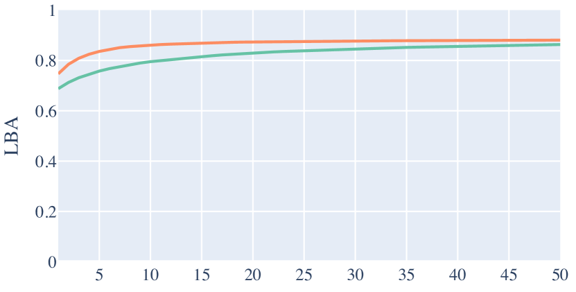
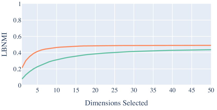
Figure 2: The average lower-bound accuracy (LBA) and lower-bound normalized mutual information (LBNMI) across all evaluated attributes and languages for fastText and BERT.

Overall, our results strongly suggest that morphosyntactic information tends to be highly focal (concentrated in a small set of dimensions) in fastText, whereas in BERT it is more dispersed. Averaging across all languages and attributes (Fig. 2), fastText has on average $0.306$ LBNMI at two dimensions, which is around twice as much as BERT at the same dimensionality. However, the difference between the two becomes progressively smaller, reducing to $0.053$ at 50 dimensions. A similar trend holds for LBA (§ 4.1), with an even smaller difference at higher dimensions. On the whole, roughly 10 dimensions are required to encode any morphosyntactic attribute we probed fastText for, compared to around 35 dimensions for BERT.

The pattern above holds across attributes (Fig. 3), and languages (Fig. 4). There is little improvement in fastText performance when adding more than 10 dimensions and, in some cases, two fastText dimensions can explain half of the information achieved when selecting 50. In contrast, while BERT also displays highly informative dimensions, a substantial increase in LBNMI can be obtained by going from 2 selected dimensions to 10 and 50. Among languages, the only exceptions to this are the Indic languages, where BERT concentrates more morphological information than fastText already at 2 dimensions. Interestingly, when looking at attributes, our results suggest that fastText encodes most attributes better than BERT (when considering the 50 most informative dimensions), except animacy, gender and number. author=adina,color=green!10,size=,fancyline,caption=,]interesting, all hierarchically low noun features. These findings also hold for LBA, where we additionally find little to no gain when comparing LBA after 50 dimensions to accuracy on the full vector.

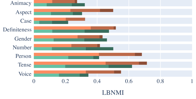
Figure 3: Comparison of per-attribute average lower-bound normalized mutual information (LBNMI) for fastText and BERT. Each bar is broken up into three components, which denote the LBNMI after selecting 2, 10 and 50 dimensions.

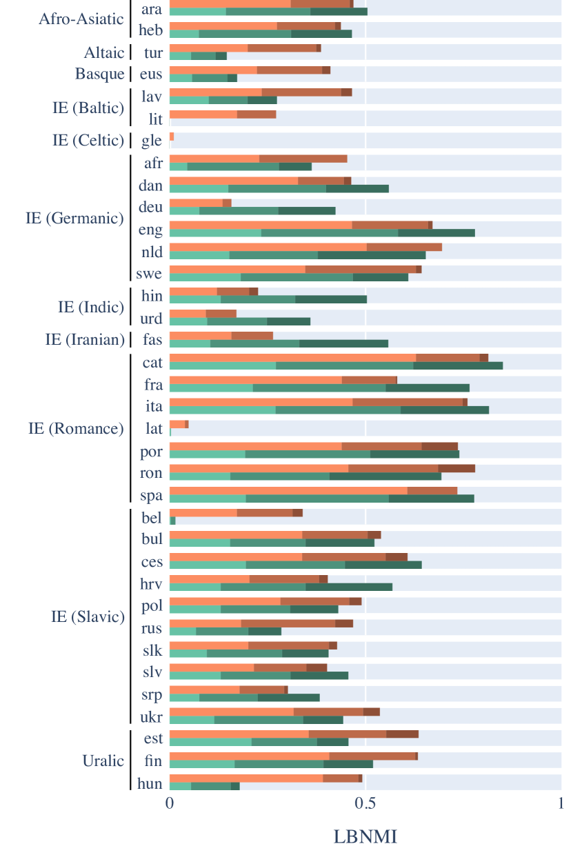
Figure 4: Comparison of per-language average lower-bound normalized mutual information (LBNMI) for fastText and BERT. Each bar is broken up into three components, which denote the LBNMI after selecting 2, 10 and 50 dimensions.

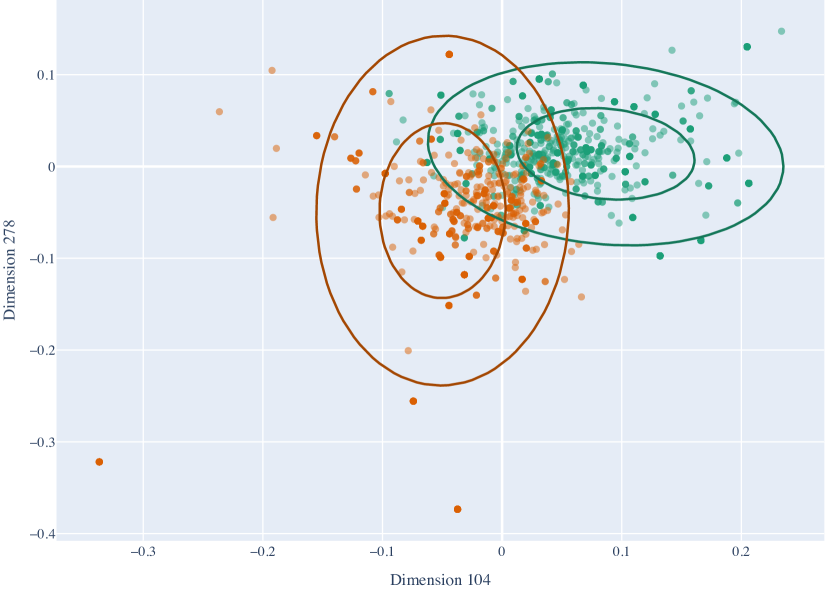
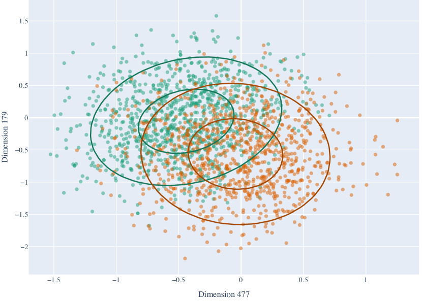
Figure 5: Scatter graph of two most informative fastText (above) and BERT (below) dimensions for English present and past tense. Contours belong to our probe.

Visualizing the most informative dimensions for BERT and fastText may give some intuition for how this trend manifests. Fig. 5 shows a scatter plot of the two most informative dimensions selected by our probe for English tense in fastText and BERT. We observed similar patterns for other morphosyntactic attributes. Both embeddings have dimensions that induce some separability in English tense, but this is more pronounced in fastText than BERT. We cannot clearly plot more than two dimensions at a time, but based on the trend depicted in Fig. 2, we can intuit that BERT makes up for at least part of the gap by inducing more separability as dimensions are added.

6.1 Limitations

The generative nature of our probe means that adequately modeling the embedding distribution $p({\boldsymbol{h}}\mid v)$ is of paramount importance. We choose a Gaussian model in order to assume as little as possible about the distribution of BERT and fastText embeddings; however, as one reviewer pointed out, the embedding distribution is unlikely to be Gaussian (see Fig. 6 for an example). author=ryan,color=violet!40,size=,fancyline,caption=,]Mention our empirical tests of this. We could do a komolgorov-smirnov test!author=lucas,color=blue!10,size=,fancyline,caption=,]we tried this, but this ended up being hard as tests are not designed for high-dimensional spaces like ours. I added a counterexample image. This results in a looser bound on the mutual information for dimensions in which the Gaussian assumption does not hold, which leads to decreasing mutual information estimates after a certain number of dimensions are selected (see Fig. 7). As we compute and report an empirical lower-bound on the mutual information for any subset of dimensions (LBMI), we have evidence that there is at least that amount of information for any given subset of dimensions. However, we expect that better modeling of the embedding distribution should improve our bound on the mutual information and thus yield a better probe (Pimentel et al., 2020b).

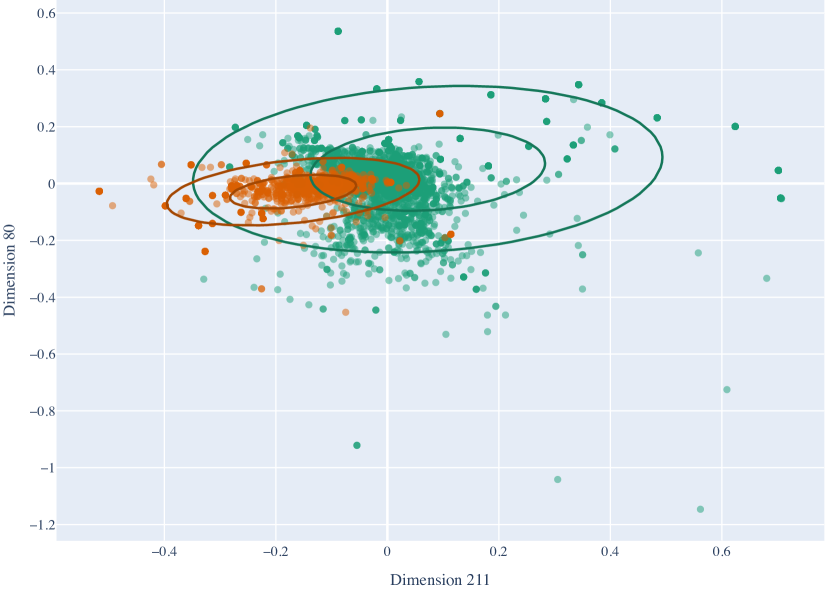
Figure 6: Two fastText dimensions that are informative for Portuguese number, but which do not appear jointly Gaussian. This dimensions pair was not favored by our Gaussian probing model; we found it by modeling $p({\boldsymbol{h}}\mid v)$ with a Gaussian–Cauchy mixture model.

7 Related Work

There has been a growing interest in understanding what information is in NLP models’ internal representations. Studies vary widely, from detailed analyses of particular scenarios and linguistic phenomena (Linzen et al., 2016; Gulordava et al., 2018; Ravfogel et al., 2018; Krasnowska-Kieraś and Wróblewska, 2019; Wallace et al., 2019; Warstadt et al., 2019; Sorodoc et al., 2020) to extensive investigations across a wealth of tasks (Tenney et al., 2018; Conneau et al., 2018; Liu et al., 2019). A plethora of methods have been designed and applied (e.g.  Li et al., 2016; Saphra and Lopez, 2019; Jumelet et al., 2019) to answer this question. Probing (Adi et al., 2017; Hupkes et al., 2018; Conneau et al., 2018) is one prominent method, which consists of using a lightly parameterized model to predict linguistic phenomena from intermediate representations, albeit recent work has raised concerns on how model parameterization and evaluation metrics may affect the effectiveness of this approach (Hewitt and Liang, 2019; Pimentel et al., 2020b; Maudslay et al., 2020; Pimentel et al., 2020a).author=ryan,color=violet!40,size=,fancyline,caption=,]We should cite our other lab’s work in this section. We cite everybody but us. Both our ACL 2020 and other EMNLP 2020 papers!author=lucas,color=blue!10,size=,fancyline,caption=,]better?

Most work in intrinsic probing has focused in the identification of individual neurons that are important for a task (Li et al., 2016; Kádár et al., 2017; Li et al., 2017; Lakretz et al., 2019). Similarly, Clark et al. (2019) and Voita et al. (2019) use probing to analyze BERT’s attention heads, finding some interpretable heads that attend to positional and syntactic features. However, there has also been some work investigating collections of neurons. For example, Shi et al. (2016) observe that different training objectives can affect how focal an intermediate representation is. Recently, Dalvi et al. (2019) use the magnitude of the weights learned by a linear probe as a proxy for dimension informativeness, and find dispersion varies depending on linguistic category. Bau et al. (2019) use unsupervised methods to find neurons that are correlated across various models, quantify said correlation, and upon manual analysis find interpretable neurons. In concurrent work in computer vision, Bau et al. (2020) identify units whose local, peak activations correlate with features in an image (e.g., material, door presence), show that ablation of these units has a disproportionately big impact on the classification of their respective features, and can be manually controlled, with interpretable effects.

Most similar to our analysis is LINSPECTOR (Şahin et al., 2020), a suite of probing tasks that includes probing for morphosyntax. Our work differs in two respects. Firstly, whereas LINSPECTOR focuses on extrinsic probing, we probe intrinsically. Secondly, the scope of our morphosyntactic study is more typologically diverse (36 vs. 5 languages), albeit they consider more varieties of word representations, such as GloVe (Pennington et al., 2014) and ELMo (Peters et al., 2018)—but not BERT.

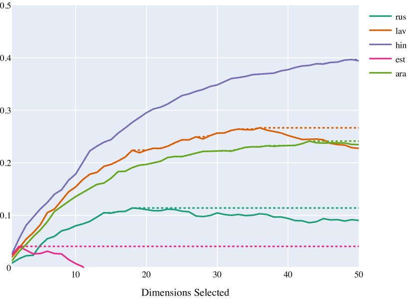
Figure 7: Plot of LBNMI (dotted) and normalized MI (solid) curves for case in 5 randomly selected languages. Note that the $y$-axis ranges from $0$–$0.5$ unlike other graphs. Observe how the normalized MI estimates start to decrease after a certain number of dimension have been selected.

8 Conclusion

author=adina,color=green!10,size=,fancyline,caption=,]the structure of this conclusion seems weird, what do you think ryanauthor=ryan,color=violet!40,size=,fancyline,caption=,]Agree should be re-written!author=lucas,color=blue!10,size=,fancyline,caption=,]Is this better?

In this paper, we introduce an alternative framework for intrinsic probing, which we term dimension selection. The idea is to use probe performance on different subsets of dimensions as a gauge for how much information about a linguistic property different subsets of dimensions jointly encode. We show that current probes are unsuitable for intrinsic probing through dimension selection as they are not inherently decomposable, which is required to make the procedure computationally tractable. Therefore, we present a decomposable probe which is based on the Gaussian distribution, and evaluate its effectiveness by probing BERT and fastText for morphosyntax across 36 languages. Overall, we find that fastText is more focal than BERT, requiring fewer dimensions to capture most of the information pertaining to a morphosyntactic property.

Future Work.

Future work will be separated into two strands. The first will focus on how to better model the distribution of embeddings given a morphosyntactic attribute; as mentioned above, this should yield a better probe overall. The second strand of work pertains to a deeper analysis of our results, and expansion to other probing tasks.author=lucas,color=blue!10,size=,fancyline,caption=,]modified last sentence

Appendix A Gaussian–inverse-Wishart Posterior Parameters

Using the notation introduced in § 3.4, the parameters of the Gaussian–inverse-Wishart distribution $\mathrm{GIW}({\boldsymbol{\mu}}_{v},\Sigma_{v}\mid{\boldsymbol{\mu}}_{n},k_{n},\Lambda_{n},\nu_{n})$, are (Murphy, 2012)

$${\boldsymbol{\mu}}_{n} =\frac{k_{0}{\boldsymbol{\mu}}_{0}+N_{v}\bar{{\boldsymbol{h}}}}{k_{n}}$$ (18)

$$k_{n} =k_{0}+N_{v}$$ (19)

$$\nu_{n} =\nu_{0}+N_{v}$$ (20)

$$\Lambda_{n} =\Lambda_{0}+S$$ (21)

$$+\frac{N_{v}k_{0}}{N_{v}+k_{0}}(\bar{{\boldsymbol{h}}}-{\boldsymbol{\mu}}_{0})(\bar{{\boldsymbol{h}}}-{\boldsymbol{\mu}}_{0})^{\top}$$

where $\bar{{\boldsymbol{h}}}$ is the empirical mean of $\mathcal{D}^{(v)}$ and $S$ is the scatter matrix

$$S=\sum_{i=1}^{N_{v}}({{\boldsymbol{h}}}^{(i)}-\bar{{\boldsymbol{h}}})({{\boldsymbol{h}}}^{(i)}-\bar{{\boldsymbol{h}}})^{\top}$$ (22)

author=lucas,color=blue!10,size=,fancyline,caption=,]Murphy Section 4.6.3.3

Appendix B Inverse-Wishart Distribution

The inverse-Wishart distribution is defined as (Murphy, 2007)

$$\mathrm{IW}(\Sigma\mid \Lambda^{-1},\nu)=\frac{1}{Z}|\Sigma|^{-\frac{\nu+d+1}{2}}$$

$$\times\exp\left(-\frac{1}{2}\mathrm{Tr}(\Lambda\Sigma^{-1})\right)$$ (23)

where

$$Z=\frac{|\Lambda|^{\frac{\nu}{2}}}{2^{\frac{\nu d}{2}}\Gamma_{d}(\frac{\nu}{2})}$$ (24)

where $\Sigma$ is a positive-definite $d\times d$ matrix, and $\Gamma_{d}$ is the multivariate Gamma function.author=lucas,color=blue!10,size=,fancyline,caption=,]Check Murphy 2007 (not the textbook) 10.5 for this formulation of the IW.

Appendix C Changes to UD Annotations

We apply some post-processing to canonicalize the automatically-converted UniMorph annotations. The changes we make are:

1. We remove any annotations with disjunctions. These constitute a minority of annotations, and handling them adequately requires language-specific knowledge.

2. We fix some annotations that we believe are typos, e.g.  replace “{CMPR}” with “CMPR”.

3. We let “PST+PRF” be a Tense annotation. This is a recurrent annotation in Latin, Romanian and Turkish.

4. We canonicalize conjunctive features by sorting them alphabetically, ensuring they all belong to the same morphological attribute, and joining them into a new feature. So the annotation “MASC+FEM” becomes “FEM+MASC”.

5. We discard language-specific annotations as this is not a canonical UniMorph dimension.

Appendix D Mutual Information Approximation

Let $V_{a}$ be a ${\mathcal{V}}_{a}$-valued random variable denoting the value of a morphosyntactic attribute, and $H$ be a $\mathbb{R}^{d}$-valued random variable for the word representation. The mutual information between $V_{a}$ and $H$ is

$$\mathrm{MI}(V_{a};H)=\mathrm{H}(V_{a})-\mathrm{H}(V_{a}\mid H)$$ (25)

To compute the entropy $\mathrm{H}(V_{a})$, we would ideally need the true attribute distribution $\overline{p}(v)$ for a language. We can empirically approximate it using $p(v)$, which has been computed from held-out data

$$\mathrm{H}(V_{a}) =\sum_{v\in\mathcal{V}_{a}}\overline{p}(v)\log_{2}\frac{1}{\overline{p}(v)}$$ (26)

$$\approx\sum_{v\in\mathcal{V}_{a}}p(v)\log_{2}\frac{1}{p(v)}$$ (27)

Computing $\mathrm{H}(V_{a}\mid H)$ is trickier as it relies on the true distribution of the representations for a value, $\overline{p}({\boldsymbol{h}}\mid v)$, which is hard to estimate as it is high-dimensional and poorly sampled in our data.

$$\mathrm{H}(V_{a}\mid H)$$ (28)

$$=\int\sum_{v\in\mathcal{V}_{a}}\overline{p}(v,{\boldsymbol{h}})\log_{2}\frac{1}{\overline{p}(v\mid{\boldsymbol{h}})}\,\mathrm{d}{\boldsymbol{h}}$$

$$=\sum_{v\in\mathcal{V}_{a}}\overline{p}(v)\int\overline{p}({\boldsymbol{h}}\mid v)\log_{2}\frac{1}{\overline{p}(v\mid{\boldsymbol{h}})}\,\mathrm{d}{\boldsymbol{h}}$$

Note that by using an approximation $\overline{p}(v\mid{\boldsymbol{h}})\approx p(v\mid{\boldsymbol{h}})$ instead (a.k.a.  our probe), we obtain an upper bound on the true conditional entropy (Brown et al., 1992)

$$\mathrm{H}(V_{a}\mid H)\leq\mathrm{H}_{p}(V_{a}\mid H)$$ (29)

$$=\sum_{v\in\mathcal{V}_{a}}\overline{p}(v)\underbrace{\int\overline{p}({\boldsymbol{h}}\mid v)\log_{2}\frac{1}{p(v\mid{\boldsymbol{h}})}\,\mathrm{d}{\boldsymbol{h}}}_{I_{v}}$$

While $\overline{p}(v)\approx p(v)$ should be reasonable for our purposes, the integral $I_{v}$ is intractable as it still depends on $\overline{p}({\boldsymbol{h}}\mid v)$. However, we can use held-out data to approximate $I_{v}$ (Pimentel et al., 2019)

$$I_{v} =-\int\overline{p}({\boldsymbol{h}}\mid v)\log_{2}p(v\mid{\boldsymbol{h}})\,\mathrm{d}{\boldsymbol{h}}$$ (30)

$$\approx-\frac{1}{N_{v}}\sum_{i=1}^{N_{v}}\log_{2}p(v\mid\tilde{{\boldsymbol{h}}}^{(i)})$$ (31)

where $\{{\tilde{{\boldsymbol{h}}}}^{(i)}\}_{i=1}^{N_{v}}$ are held-out word representations for a value $v$, and thus obtain an empirical upper-bound on $\mathrm{H}(V_{a}\mid H)$.

Appendix E Reproducibility Details

All experiments were run on an AWS p2.xlarge instance, with 1 Tesla K80 GPU, 4 CPU cores, and 61 GB of RAM. The total runtime of the experiments was 2 days, 18 hours, 42 minutes and 14 seconds.

In total, when considering a $d$-dimensional word representation, this model has

$$\underbrace{|{\mathcal{V}}_{a}|\left(\frac{d(d+1)}{2}+d\right)}_{\text{Gaussians}}+\underbrace{\left(|{\mathcal{V}}_{a}|-1\right)}_{\text{Categorical}}$$ (32)

parameters. In practice, this means that for every value, a fastText Gaussian we fit has $45450$ parameters, whereas a BERT Gaussian has $296064$ parameters.

Appendix F Probed Attributes by Language

App. F shows a list of all languages that were probed, which attributes were probed, and which values were considered. The number of example words for a value in the train/validation/test split is shown in parenthesis.

Table of attributes that were probed for each language, and the values that were considered for that attribute. The number of example words for a value in the train/validation/test split is shown in parenthesis.
Language	Attribute	Values
Language	Attribute	Values
(Continued next page)          afr (Afrikaans)	Number	PL (2682/399/1067), SG (6390/999/1656)
ara (Arabic)	Number	PL (18193/2282/2411), SG (97436/12692/12451)
	Gender and Noun Class	FEM (22104/2666/2842), MASC (27953/3982/3639)
	Mood	IND (6452/832/774), SBJV (1021/157/135)
	Aspect	IPFV (7986/1050/999), PFV (8951/1292/1226)
	Voice	ACT (16039/2169/2081), PASS (898/173/144)
	Case	ACC (21975/2951/2857), GEN (70767/8920/9137), NOM (13901/1859/1668)
	Definiteness	DEF (47204/5785/6077), INDF (21122/3004/2668)
bel (Belarusian)	Case	GEN (912/336/262), NOM (673/174/171)
	Gender and Noun Class	FEM (910/270/194), MASC (1059/344/351)
	Number	PL (781/259/212), SG (2208/639/615)
bul (Bulgarian)	Gender and Noun Class	FEM (16442/2142/2119), MASC (21236/2614/2650), NEUT (9292/1271/1214)
	Number	PL (18973/2443/2371), SG (49940/6427/6388)
	Definiteness	DEF (15310/1939/1942), INDF (33516/4340/4232)
	Tense	PRS (10781/1405/1330), PST (5373/677/716)
	Person	1 (2548/353/345), 3 (14882/1885/1824)
	Voice	ACT (1885/239/222), PASS (1625/221/204)
cat (Catalan)	Gender and Noun Class	FEM (66961/9409/9368), MASC (85011/11313/11473)
	Number	PL (54636/7105/7314), SG (150183/20733/20682)
	Mood	IND (27555/3678/3662), SBJV (2070/303/252)
	Tense	FUT (3005/319/405), PRS (25110/3347/3347), PST (8398/1236/1040)
ces (Czech)	Case	ACC (140691/19275/20747), DAT (31793/4458/4605), ESS (104763/14467/15519), GEN (176912/23678/25261), INS (53879/7312/8282), NOM (158994/21358/23042)
	Gender and Noun Class	FEM (88003/11924/13173), MASC (137896/18345/19153), NEUT (44566/6295/6682)
	Comparison	CMPR (6134/826/908), RL (3199/442/494)
	Number	PL (180092/24725/26325), SG (459202/62398/67686)
	Person	1 (12691/1993/2293), 2 (1973/342/471), 3 (68973/9461/10390)
	Aspect	IPFV (41460/5706/6268), PFV (29944/4151/4408)
	Tense	PRS (64246/8849/10059), PST (44390/6089/6523)
	Polarity	NEG (16126/2172/2361), POS (86217/11270/12221)
	Animacy	ANIM (55084/7179/7543), INAN (62155/8469/8955)
	Voice	ACT (3549/410/539), PASS (7426/1044/1056)
dan (Danish)	Gender and Noun Class	FEM+MASC (16075/2045/1981), NEUT (7294/964/872)
	Definiteness	DEF (5218/664/655), INDF (14149/1867/1682)
	Number	PL (7332/1050/909), SG (21782/2784/2639)
	Tense	PRS (5806/753/679), PST (4017/575/604)
deu (German)	Number	PL (17392/1009/1259), SG (78706/3789/4698)
	Case	ACC (20352/1243/1480), DAT (29961/1150/1694), GEN (5675/195/314), NOM (28192/1528/1729)
eng (English)	Number	PL (12599/1376/1364), SG (55978/7192/7266)
	Tense	PRS (8129/1063/940), PST (9359/996/981)
est (Estonian)	Case	ABL+IN (1383/155/169), ALL+AT (1299/154/175), ALL+IN (1451/166/188), AT+ESS (1813/241/221), COM (1011/131/129), ESS+IN (1757/210/215), GEN (8808/1081/1132), NOM (13955/1727/1683), PRT (5022/572/628)
	Number	PL (8434/1052/1001), SG (38059/4655/4801)
	Finiteness	FIN (11753/1462/1501), NFIN (1306/181/170)
	Tense	PRS (5633/670/680), PST (6734/894/856)
	Person	1 (2240/252/312), 3 (9058/1175/1144)
eus (Basque)	Case	ABL+AT (532/163/187), ABS (10459/3457/3465), ALL+AT (514/181/169), COM (383/128/148), DAT (745/232/239), ERG (2670/859/873), ESS (3148/977/1024), ESS+IN (3408/1167/1180), GEN (2334/763/806), INS (633/235/203), PRT (420/135/162)
	Animacy	ANIM (778/274/236), INAN (7269/2375/2521)
	Definiteness	DEF (19134/6315/6336), INDF (3688/1244/1224)
	Number	PL (4162/1393/1376), SG (15257/5017/5057)
	Aspect	IPFV (1062/363/395), PFV (3476/1149/1140), PROG (2937/914/967), PROSP (953/297/279)
fas (Persian)	Number	PL (11152/1250/1327), SG (50635/7040/7105)
fin (Finnish)	Number	PL (21315/2356/2878), SG (79259/8978/9967)
	Case	ABL+IN (4204/487/531), ALL+AT (1909/236/254), ALL+IN (5014/539/616), AT+ESS (3310/375/384), ESS+IN (5508/600/661), FRML (1974/214/261), GEN (20002/2299/2490), NOM (25818/2905/3252), PRT (12638/1404/1709), TRANS (1206/111/139)
	Voice	ACT (23469/2626/3082), PASS (4179/505/542)
	Tense	PRS (11149/1314/1732), PST (9039/980/958)
	Person	1 (3104/363/412), 3 (15218/1746/2007)
fra (French)	Gender and Noun Class	FEM (63408/6471/1623), MASC (81523/8352/2439)
	Number	PL (41157/4146/1286), SG (131994/13416/3681)
	Tense	PRS (19256/1864/589), PST (14020/1382/343)
gle (Irish)	Gender and Noun Class	FEM (327/1240/1158), MASC (690/2188/2208)
	Number	PL (177/752/594), SG (1181/3841/3841)
heb (Hebrew)	Definiteness	DEF (2184/174/156), INDF (21817/1812/2069)
	Number	PL (14478/1328/1280), SG (38263/3182/3650)
hin (Hindi)	Number	PL (24553/3049/2932), SG (149419/18658/19128)
	Case	ACC (79132/9903/10138), NOM (66735/8392/8437)
	Gender and Noun Class	FEM (43951/5496/5686), MASC (104389/13116/13253)
hrv (Croatian)	Gender and Noun Class	FEM (31053/3094/2468), MASC (41905/3285/3084), NEUT (12411/921/1070)
	Number	PL (27716/2672/2583), SG (74308/5976/5357)
	Case	ACC (22562/2038/1721), DAT (2332/197/171), ESS (14876/1335/1182), GEN (27281/2552/2163), INS (5388/366/398), NOM (26435/2125/2046)
	Tense	PRS (15665/1298/1299), PST (6537/509/436)
	Finiteness	FIN (16468/1349/1326), NFIN (3331/288/273)
hun (Hungarian)	Definiteness	DEF (2885/1770/1524), INDF (1307/577/619)
	Number	PL (1516/850/744), SG (9948/5853/5223)
	Case	ACC (935/541/484), ALL+ON (248/162/157), ESS+IN (478/248/242), INS (218/198/155), NOM (6492/3910/3352)
	Possession	PSS3S (1139/775/652), PSSD (5676/2779/2353)
	Tense	PRS (956/513/369), PST (795/357/533)
ita (Italian)	Gender and Noun Class	FEM (44923/1947/1713), MASC (59063/2613/2265)
	Number	PL (38689/1739/1321), SG (95035/4138/3843)
	Tense	PRS (15854/693/620), PST (11200/491/432)
lat (Latin)	Number	PL (1237/2086/1757), SG (3726/4029/4883)
	Case	ABL+AT (944/1150/999), ACC (1369/1545/1813), DAT (231/306/270), GEN (492/451/324), NOM (809/1353/1436)
	Gender and Noun Class	FEM (517/721/621), MASC (912/1187/1150), NEUT (378/570/525)
	Person	1 (179/166/324), 3 (837/892/1232)
	Tense	PRS (694/1020/1224), PST (815/764/1047)
	Mood	IND (868/939/1431), SBJV (212/255/270)
	Aspect	IPFV (138/209/246), PFV (689/567/814)
lav (Latvian)	Case	ACC (5729/1113/1139), DAT (2999/622/610), ESS (3148/619/704), GEN (7251/1343/1311), NOM (10222/2257/2300)
	Number	PL (8157/1494/1678), SG (21128/4474/4517)
	Gender and Noun Class	FEM (5243/987/1029), MASC (6252/1276/1319)
	Tense	PRS (4629/838/1129), PST (3673/1015/749)
	Person	1 (1539/436/450), 3 (6449/1368/1332)
lit (Lithuanian)	Case	GEN (356/153/150), NOM (504/164/152)
	Gender and Noun Class	FEM (496/162/159), MASC (805/282/296)
	Number	PL (459/180/215), SG (1176/373/342)
nld (Dutch)	Number	PL (10797/615/793), SG (42640/2850/2609)
	Finiteness	FIN (17418/1023/903), NFIN (5213/242/407)
	Gender and Noun Class	FEM+MASC (18298/1316/1225), NEUT (10238/687/690)
pol (Polish)	Case	ACC (7083/1188/1278), ESS (5790/859/876), GEN (10429/1663/1773), INS (2616/502/463), NOM (7575/1228/1268)
	Number	PL (9871/1491/1573), SG (25225/4242/4454)
	Gender and Noun Class	FEM (4083/678/755), MASC (7858/1306/1380), NEUT (2416/371/409)
	Animacy	HUM (4285/663/755), INAN (1641/268/309)
	Tense	PRS (3823/634/660), PST (3547/621/645)
	Person	1 (1501/261/332), 3 (3725/613/603)
por (Portuguese)	Number	PL (27002/1366/1299), SG (92097/5125/4723)
	Gender and Noun Class	FEM (40907/2138/2107), MASC (57079/3154/2850)
	Tense	PRS (8438/512/466), PST (9107/470/449)
ron (Romanian)	Definiteness	DEF (24561/2326/2199), INDF (33780/3142/2992)
	Number	PL (28550/2558/2430), SG (66435/6248/6013)
	Mood	IND (11099/1000/975), SBJV (3623/390/329)
	Gender and Noun Class	FEM (17544/1687/1510), MASC (14229/1315/1333)
rus (Russian)	Animacy	ANIM (7032/1184/1156), INAN (32548/5037/4869)
	Case	ACC (5262/831/834), DAT (1732/207/248), ESS (5066/751/807), GEN (13687/2201/2089), INS (3041/452/428), NOM (12342/2017/1831)
	Gender and Noun Class	FEM (11145/1842/1762), MASC (21073/3360/3309), NEUT (6774/961/953)
	Number	PL (9691/1432/1413), SG (34647/5518/5385)
	Tense	PRS (1870/293/275), PST (4227/631/677)
	Aspect	IPFV (3978/602/619), PFV (3133/481/498)
	Voice	MID (1326/192/208), PASS (1125/178/173)
slk (Slovak)	Gender and Noun Class	FEM (14217/2249/2566), MASC (17129/3838/3450), NEUT (6817/992/1306)
	Number	PL (8989/1635/2013), SG (36266/5750/5840)
	Case	ACC (9651/1392/1466), DAT (2031/328/271), ESS (5062/1203/1151), GEN (7228/1867/1998), INS (3108/699/698), NOM (10605/1869/2131)
	Tense	PRS (4926/282/491), PST (8271/950/823)
	Aspect	IPFV (8561/705/898), PFV (6003/608/524)
	Animacy	ANIM (8769/2069/1401), INAN (8360/1769/2049)
slv (Slovenian)	Case	ACC (13762/1794/1709), DAT (2219/236/257), ESS (10546/1448/1273), GEN (12424/1667/1545), INS (4713/673/630), NOM (13405/1615/1730)
	Gender and Noun Class	FEM (9549/1149/1231), MASC (13512/1642/1626), NEUT (4732/597/610)
	Number	PL (18042/2692/2286), SG (44944/5221/5650)
	Person	1 (2120/275/253), 3 (11322/1247/1485)
	Finiteness	FIN (12361/1474/1568), NFIN (1083/163/146)
	Aspect	IPFV (4774/580/649), PFV (5233/602/623)
spa (Spanish)	Number	PL (47382/4347/1471), SG (139165/13604/4494)
	Gender and Noun Class	FEM (60665/5724/1857), MASC (79816/7849/2522)
	Tense	PRS (16120/1520/644), PST (13814/1336/381)
srp (Serbian)	Number	PL (10057/1606/1754), SG (31875/4781/5141)
	Gender and Noun Class	FEM (12944/1928/2193), MASC (17331/2597/2793), NEUT (4187/621/626)
	Case	ACC (8294/1329/1407), DAT (866/126/163), ESS (5804/882/1038), GEN (10910/1547/1745), INS (2029/262/261), NOM (11456/1748/1816)
swe (Swedish)	Gender and Noun Class	FEM+MASC (4813/757/1403), NEUT (2730/457/840)
	Number	PL (8110/1254/2721), SG (18229/2638/5248)
	Definiteness	DEF (10447/1775/3192), INDF (17005/2321/5116)
tur (Turkish)	Case	ABL+AT (709/175/183), ACC (1688/428/451), DAT (1837/436/489), ESS (1415/361/359), GEN (1540/380/385), INS (515/139/123), NOM (8690/2288/2362)
	Aspect	IPFV (722/232/214), PFV (6156/1589/1671), PROG (887/248/225)
	Person	1 (1433/392/348), 2 (624/189/147), 3 (7013/1867/1880)
	Tense	PRS (3563/945/963), PST (2941/733/757)
	Number	PL (2737/687/729), SG (16222/4262/4283)
	Possession	PSS1S (531/126/141), PSS3S (4035/982/1053)
	Polarity	NEG (782/227/237), POS (6410/1694/1713)
ukr (Ukrainian)	Case	ACC (8908/1196/1681), ESS (4895/656/997), GEN (12499/2087/3397), INS (3953/505/843), NOM (9919/1398/1831)
	Number	PL (11432/1507/2215), SG (28210/4031/6016)
	Gender and Noun Class	FEM (4716/556/1035), MASC (6245/890/1294), NEUT (2600/318/477)
	Animacy	ANIM (2671/316/447), INAN (2696/407/615)
	Tense	PRS (2505/397/454), PST (4093/380/535)
urd (Urdu)	Number	PL (8105/1008/844), SG (58067/7841/8254)
	Case	ACC (29707/4210/4112), NOM (29217/3853/4264)

References

- Adi et al. (2017) Yossi Adi, Einat Kermany, Yonatan Belinkov, Ofer Lavi, and Yoav Goldberg. 2017. Fine-grained analysis of sentence embeddings using auxiliary prediction tasks. In 5th International Conference on Learning Representations, ICLR 2017, Toulon, France, April 24-26, 2017, Conference Track Proceedings. OpenReview.net.
- Alain and Bengio (2017) Guillaume Alain and Yoshua Bengio. 2017. Understanding intermediate layers using linear classifier probes. In The 5th International Conference on Learning Representations.
- Bau et al. (2019) Anthony Bau, Yonatan Belinkov, Hassan Sajjad, Nadir Durrani, Fahim Dalvi, and James Glass. 2019. Identifying and controlling important neurons in neural machine translation. In International Conference on Learning Representations.
- Bau et al. (2020) David Bau, Jun-Yan Zhu, Hendrik Strobelt, Agata Lapedriza, Bolei Zhou, and Antonio Torralba. 2020. Understanding the role of individual units in a deep neural network. Proceedings of the National Academy of Sciences.
- Belinkov et al. (2017) Yonatan Belinkov, Nadir Durrani, Fahim Dalvi, Hassan Sajjad, and James Glass. 2017. What do neural machine translation models learn about morphology? In Proceedings of the 55th Annual Meeting of the Association for Computational Linguistics (Volume 1: Long Papers), pages 861–872, Vancouver, Canada. Association for Computational Linguistics.
- Belinkov and Glass (2019) Yonatan Belinkov and James Glass. 2019. Analysis methods in neural language processing: A survey. Transactions of the Association for Computational Linguistics, 7:49–72.
- Binshtok et al. (2007) Maxim Binshtok, Ronen I. Brafman, Solomon E. Shimony, Ajay Martin, and Craig Boutilier. 2007. Computing optimal subsets. In Proceedings of the 22nd National Conference on Artificial Intelligence - Volume 2, AAAI’07, pages 1231–1236, Vancouver, British Columbia, Canada. AAAI Press.
- Bojanowski et al. (2017) Piotr Bojanowski, Edouard Grave, Armand Joulin, and Tomas Mikolov. 2017. Enriching word vectors with subword information. Transactions of the Association for Computational Linguistics, 5:135–146.
- Bouton et al. (2018) Sophie Bouton, Valérian Chambon, Rémi Tyrand, Adrian G Guggisberg, Margitta Seeck, Sami Karkar, Dimitri Van De Ville, and Anne-Lise Giraud. 2018. Focal versus distributed temporal cortex activity for speech sound category assignment. Proceedings of the National Academy of Sciences, 115(6):E1299–E1308.
- Brown et al. (1992) Peter F. Brown, Stephen A. Della Pietra, Vincent J. Della Pietra, Jennifer C. Lai, and Robert L. Mercer. 1992. An estimate of an upper bound for the entropy of English. Computational Linguistics, 18(1):31–40.
- Clark et al. (2019) Kevin Clark, Urvashi Khandelwal, Omer Levy, and Christopher D. Manning. 2019. What does BERT look at? An analysis of BERT’s attention. In Proceedings of the 2019 ACL Workshop BlackboxNLP: Analyzing and Interpreting Neural Networks for NLP, pages 276–286, Florence, Italy. Association for Computational Linguistics.
- Conneau et al. (2018) Alexis Conneau, German Kruszewski, Guillaume Lample, Loïc Barrault, and Marco Baroni. 2018. What you can cram into a single $&!#* vector: Probing sentence embeddings for linguistic properties. In Proceedings of the 56th Annual Meeting of the Association for Computational Linguistics (Volume 1: Long Papers), pages 2126–2136, Melbourne, Australia. Association for Computational Linguistics.
- Dalvi et al. (2019) Fahim Dalvi, Nadir Durrani, Hassan Sajjad, Yonatan Belinkov, Anthony Bau, and James Glass. 2019. What is one grain of sand in the desert? Analyzing individual neurons in deep NLP models. Proceedings of the AAAI Conference on Artificial Intelligence, 33:6309–6317.
- Devlin et al. (2019) Jacob Devlin, Ming-Wei Chang, Kenton Lee, and Kristina Toutanova. 2019. BERT: Pre-training of deep bidirectional transformers for language understanding. In Proceedings of the 2019 Conference of the North American Chapter of the Association for Computational Linguistics: Human Language Technologies, Volume 1 (Long and Short Papers), pages 4171–4186, Minneapolis, Minnesota. Association for Computational Linguistics.
- Fraley and Raftery (2007) Chris Fraley and Adrian E. Raftery. 2007. Bayesian regularization for normal mixture estimation and model-based clustering. Journal of Classification, 24:155–181.
- Gates et al. (2019) Alexander J. Gates, Ian B. Wood, William P. Hetrick, and Yong-Yeol Ahn. 2019. Element-centric clustering comparison unifies overlaps and hierarchy. Scientific Reports, 9(8574).
- Giulianelli et al. (2018) Mario Giulianelli, Jack Harding, Florian Mohnert, Dieuwke Hupkes, and Willem Zuidema. 2018. Under the hood: Using diagnostic classifiers to investigate and improve how language models track agreement information. In Proceedings of the 2018 EMNLP Workshop BlackboxNLP: Analyzing and Interpreting Neural Networks for NLP, pages 240–248, Brussels, Belgium. Association for Computational Linguistics.
- Grave et al. (2018) Edouard Grave, Piotr Bojanowski, Prakhar Gupta, Armand Joulin, and Tomas Mikolov. 2018. Learning word vectors for 157 languages. In Proceedings of the Eleventh International Conference on Language Resources and Evaluation (LREC 2018), Miyazaki, Japan. European Language Resources Association (ELRA).
- Gulordava et al. (2018) Kristina Gulordava, Piotr Bojanowski, Edouard Grave, Tal Linzen, and Marco Baroni. 2018. Colorless green recurrent networks dream hierarchically. In Proceedings of the 2018 Conference of the North American Chapter of the Association for Computational Linguistics: Human Language Technologies, Volume 1 (Long Papers), pages 1195–1205, New Orleans, Louisiana. Association for Computational Linguistics.
- Hewitt and Liang (2019) John Hewitt and Percy Liang. 2019. Designing and interpreting probes with control tasks. In Proceedings of the 2019 Conference on Empirical Methods in Natural Language Processing and the 9th International Joint Conference on Natural Language Processing (EMNLP-IJCNLP), pages 2733–2743, Hong Kong, China. Association for Computational Linguistics.
- Hewitt and Manning (2019) John Hewitt and Christopher D. Manning. 2019. A structural probe for finding syntax in word representations. In Proceedings of the 2019 Conference of the North American Chapter of the Association for Computational Linguistics: Human Language Technologies, Volume 1 (Long and Short Papers), pages 4129–4138, Minneapolis, Minnesota. Association for Computational Linguistics.
- Hupkes et al. (2018) Dieuwke Hupkes, Sara Veldhoen, and Willem Zuidema. 2018. Visualisation and ’diagnostic classifiers’ reveal how recurrent and recursive neural networks process hierarchical structure. Journal of Artificial Intelligence Research, 61:907–926.
- Jaynes (2003) Edwin T. Jaynes. 2003. Probability Theory: The Logic of Science. Cambridge University Press, Cambridge.
- Joshi et al. (2019) Mandar Joshi, Omer Levy, Luke Zettlemoyer, and Daniel Weld. 2019. BERT for coreference resolution: Baselines and analysis. In Proceedings of the 2019 Conference on Empirical Methods in Natural Language Processing and the 9th International Joint Conference on Natural Language Processing (EMNLP-IJCNLP), pages 5802–5807, Hong Kong, China. Association for Computational Linguistics.
- Jumelet et al. (2019) Jaap Jumelet, Willem Zuidema, and Dieuwke Hupkes. 2019. Analysing neural language models: Contextual decomposition reveals default reasoning in number and gender assignment. In Proceedings of the 23rd Conference on Computational Natural Language Learning (CoNLL), pages 1–11, Hong Kong, China. Association for Computational Linguistics.
- Kádár et al. (2017) Ákos Kádár, Grzegorz Chrupała, and Afra Alishahi. 2017. Representation of linguistic form and function in recurrent neural networks. Computational Linguistics, 43(4):761–780.
- Karpathy et al. (2015) Andrej Karpathy, Justin Johnson, and Li Fei-Fei. 2015. Visualizing and understanding recurrent networks. arXiv:1506.02078 [cs].
- Kim et al. (2019) Najoung Kim, Roma Patel, Adam Poliak, Patrick Xia, Alex Wang, Tom McCoy, Ian Tenney, Alexis Ross, Tal Linzen, Benjamin Van Durme, Samuel R. Bowman, and Ellie Pavlick. 2019. Probing what different NLP tasks teach machines about function word comprehension. In Proceedings of the Eighth Joint Conference on Lexical and Computational Semantics (*SEM 2019), pages 235–249, Minneapolis, Minnesota. Association for Computational Linguistics.
- Kirov et al. (2018) Christo Kirov, Ryan Cotterell, John Sylak-Glassman, Géraldine Walther, Ekaterina Vylomova, Patrick Xia, Manaal Faruqui, Sebastian Mielke, Arya McCarthy, Sandra Kübler, David Yarowsky, Jason Eisner, and Mans Hulden. 2018. UniMorph 2.0: Universal morphology. In Proceedings of the Eleventh International Conference on Language Resources and Evaluation (LREC 2018), Miyazaki, Japan. European Language Resources Association (ELRA).
- Kitaev et al. (2019) Nikita Kitaev, Steven Cao, and Dan Klein. 2019. Multilingual constituency parsing with self-attention and pre-training. In Proceedings of the 57th Annual Meeting of the Association for Computational Linguistics, pages 3499–3505, Florence, Italy. Association for Computational Linguistics.
- Kleinberg and Tardos (2005) Jon Kleinberg and Éva Tardos. 2005. Algorithm Design. Addison-Wesley Longman Publishing Co., Inc., USA.
- Kondratyuk (2019) Dan Kondratyuk. 2019. Cross-lingual lemmatization and morphology tagging with two-stage multilingual BERT fine-tuning. In Proceedings of the 16th Workshop on Computational Research in Phonetics, Phonology, and Morphology, pages 12–18, Florence, Italy. Association for Computational Linguistics.
- Krasnowska-Kieraś and Wróblewska (2019) Katarzyna Krasnowska-Kieraś and Alina Wróblewska. 2019. Empirical linguistic study of sentence embeddings. In Proceedings of the 57th Annual Meeting of the Association for Computational Linguistics, pages 5729–5739, Florence, Italy. Association for Computational Linguistics.
- Lakretz et al. (2019) Yair Lakretz, German Kruszewski, Theo Desbordes, Dieuwke Hupkes, Stanislas Dehaene, and Marco Baroni. 2019. The emergence of number and syntax units in LSTM language models. In Proceedings of the 2019 Conference of the North American Chapter of the Association for Computational Linguistics: Human Language Technologies, Volume 1 (Long and Short Papers), pages 11–20, Minneapolis, Minnesota. Association for Computational Linguistics.
- Li et al. (2016) Jiwei Li, Xinlei Chen, Eduard Hovy, and Dan Jurafsky. 2016. Visualizing and understanding neural models in NLP. In Proceedings of the 2016 Conference of the North American Chapter of the Association for Computational Linguistics: Human Language Technologies, pages 681–691, San Diego, California. Association for Computational Linguistics.
- Li et al. (2017) Jiwei Li, Will Monroe, and Dan Jurafsky. 2017. Understanding neural networks through representation erasure. arXiv:1612.08220 [cs].
- Lin et al. (2019) Yongjie Lin, Yi Chern Tan, and Robert Frank. 2019. Open sesame: Getting inside BERT’s linguistic knowledge. In Proceedings of the 2019 ACL Workshop BlackboxNLP: Analyzing and Interpreting Neural Networks for NLP, pages 241–253, Florence, Italy. Association for Computational Linguistics.
- Linzen et al. (2016) Tal Linzen, Emmanuel Dupoux, and Yoav Goldberg. 2016. Assessing the ability of LSTMs to learn syntax-sensitive dependencies. Transactions of the Association for Computational Linguistics, 4:521–535.
- Liu et al. (2019) Nelson F. Liu, Matt Gardner, Yonatan Belinkov, Matthew E. Peters, and Noah A. Smith. 2019. Linguistic knowledge and transferability of contextual representations. In Proceedings of the 2019 Conference of the North American Chapter of the Association for Computational Linguistics: Human Language Technologies, Volume 1 (Long and Short Papers), pages 1073–1094, Minneapolis, Minnesota. Association for Computational Linguistics.
- Maudslay et al. (2020) Rowan Hall Maudslay, Josef Valvoda, Tiago Pimentel, Adina Williams, and Ryan Cotterell. 2020. A tale of a probe and a parser. In Proceedings of the 58th Annual Meeting of the Association for Computational Linguistics. Association for Computational Linguistics.
- McCarthy et al. (2018) Arya D. McCarthy, Miikka Silfverberg, Ryan Cotterell, Mans Hulden, and David Yarowsky. 2018. Marrying universal dependencies and universal morphology. In Proceedings of the Second Workshop on Universal Dependencies (UDW 2018), pages 91–101, Brussels, Belgium. Association for Computational Linguistics.
- Murphy (2007) Kevin P. Murphy. 2007. Conjugate Bayesian analysis of the Gaussian distribution. Technical report, University of British Columbia.
- Murphy (2012) Kevin P. Murphy. 2012. Machine Learning: A Probabilistic Perspective. Adaptive Computation and Machine Learning Series. MIT Press, Cambridge, MA.
- Nivre et al. (2017) Joakim Nivre, Željko Agić, Lars Ahrenberg, Lene Antonsen, Maria Jesus Aranzabe, Masayuki Asahara, Luma Ateyah, Mohammed Attia, Aitziber Atutxa, Liesbeth Augustinus, Elena Badmaeva, Miguel Ballesteros, Esha Banerjee, Sebastian Bank, Verginica Barbu Mititelu, John Bauer, Kepa Bengoetxea, Riyaz Ahmad Bhat, Eckhard Bick, Victoria Bobicev, Carl Börstell, Cristina Bosco, Gosse Bouma, Sam Bowman, Aljoscha Burchardt, Marie Candito, Gauthier Caron, Gülşen Cebiroğlu Eryiğit, Giuseppe G. A. Celano, Savas Cetin, Fabricio Chalub, Jinho Choi, Silvie Cinková, Çağrı Çöltekin, Miriam Connor, Elizabeth Davidson, Marie-Catherine de Marneffe, Valeria de Paiva, Arantza Diaz de Ilarraza, Peter Dirix, Kaja Dobrovoljc, Timothy Dozat, Kira Droganova, Puneet Dwivedi, Marhaba Eli, Ali Elkahky, Tomaž Erjavec, Richárd Farkas, Hector Fernandez Alcalde, Jennifer Foster, Cláudia Freitas, Katarína Gajdošová, Daniel Galbraith, Marcos Garcia, Moa Gärdenfors, Kim Gerdes, Filip Ginter, Iakes Goenaga, Koldo Gojenola, Memduh Gökırmak, Yoav Goldberg, Xavier Gómez Guinovart, Berta Gonzáles Saavedra, Matias Grioni, Normunds Grūzītis, Bruno Guillaume, Nizar Habash, Jan Hajič, Jan Hajič jr., Linh Hà Mỹ, Kim Harris, Dag Haug, Barbora Hladká, Jaroslava Hlaváčová, Florinel Hociung, Petter Hohle, Radu Ion, Elena Irimia, Tomáš Jelínek, Anders Johannsen, Fredrik Jørgensen, Hüner Kaşıkara, Hiroshi Kanayama, Jenna Kanerva, Tolga Kayadelen, Václava Kettnerová, Jesse Kirchner, Natalia Kotsyba, Simon Krek, Veronika Laippala, Lorenzo Lambertino, Tatiana Lando, John Lee, Phương Lê Hồng, Alessandro Lenci, Saran Lertpradit, Herman Leung, Cheuk Ying Li, Josie Li, Keying Li, Nikola Ljubešić, Olga Loginova, Olga Lyashevskaya, Teresa Lynn, Vivien Macketanz, Aibek Makazhanov, Michael Mandl, Christopher Manning, Cătălina Mărănduc, David Mareček, Katrin Marheinecke, Héctor Martínez Alonso, André Martins, Jan Mašek, Yuji Matsumoto, Ryan McDonald, Gustavo Mendonça, Niko Miekka, Anna Missilä, Cătălin Mititelu, Yusuke Miyao, Simonetta Montemagni, Amir More, Laura Moreno Romero, Shinsuke Mori, Bohdan Moskalevskyi, Kadri Muischnek, Kaili Müürisep, Pinkey Nainwani, Anna Nedoluzhko, Gunta Nešpore-Bērzkalne, Lương Nguyễn Thị, Huyền Nguyễn Thị Minh, Vitaly Nikolaev, Hanna Nurmi, Stina Ojala, Petya Osenova, Robert Östling, Lilja Øvrelid, Elena Pascual, Marco Passarotti, Cenel-Augusto Perez, Guy Perrier, Slav Petrov, Jussi Piitulainen, Emily Pitler, Barbara Plank, Martin Popel, Lauma Pretkalniņa, Prokopis Prokopidis, Tiina Puolakainen, Sampo Pyysalo, Alexandre Rademaker, Loganathan Ramasamy, Taraka Rama, Vinit Ravishankar, Livy Real, Siva Reddy, Georg Rehm, Larissa Rinaldi, Laura Rituma, Mykhailo Romanenko, Rudolf Rosa, Davide Rovati, Benoît Sagot, Shadi Saleh, Tanja Samardžić, Manuela Sanguinetti, Baiba Saulīte, Sebastian Schuster, Djamé Seddah, Wolfgang Seeker, Mojgan Seraji, Mo Shen, Atsuko Shimada, Dmitry Sichinava, Natalia Silveira, Maria Simi, Radu Simionescu, Katalin Simkó, Mária Šimková, Kiril Simov, Aaron Smith, Antonio Stella, Milan Straka, Jana Strnadová, Alane Suhr, Umut Sulubacak, Zsolt Szántó, Dima Taji, Takaaki Tanaka, Trond Trosterud, Anna Trukhina, Reut Tsarfaty, Francis Tyers, Sumire Uematsu, Zdeňka Urešová, Larraitz Uria, Hans Uszkoreit, Sowmya Vajjala, Daniel van Niekerk, Gertjan van Noord, Viktor Varga, Eric Villemonte de la Clergerie, Veronika Vincze, Lars Wallin, Jonathan North Washington, Mats Wirén, Tak-sum Wong, Zhuoran Yu, Zdeněk Žabokrtský, Amir Zeldes, Daniel Zeman, and Hanzhi Zhu. 2017. Universal dependencies 2.1. LINDAT/CLARIAH-CZ digital library at the Institute of Formal and Applied Linguistics (ÚFAL), Faculty of Mathematics and Physics, Charles University.
- Pennington et al. (2014) Jeffrey Pennington, Richard Socher, and Christopher Manning. 2014. GloVe: Global vectors for word representation. In Proceedings of the 2014 Conference on Empirical Methods in Natural Language Processing (EMNLP), pages 1532–1543, Doha, Qatar. Association for Computational Linguistics.
- Peters et al. (2018) Matthew Peters, Mark Neumann, Mohit Iyyer, Matt Gardner, Christopher Clark, Kenton Lee, and Luke Zettlemoyer. 2018. Deep contextualized word representations. In Proceedings of the 2018 Conference of the North American Chapter of the Association for Computational Linguistics: Human Language Technologies, Volume 1 (Long Papers), pages 2227–2237, New Orleans, Louisiana. Association for Computational Linguistics.
- Pimentel et al. (2019) Tiago Pimentel, Arya D. McCarthy, Damian Blasi, Brian Roark, and Ryan Cotterell. 2019. Meaning to form: Measuring systematicity as information. In Proceedings of the 57th Annual Meeting of the Association for Computational Linguistics, pages 1751–1764, Florence, Italy. Association for Computational Linguistics.
- Pimentel et al. (2020a) Tiago Pimentel, Naomi Saphra, Adina Williams, and Ryan Cotterell. 2020a. Pareto probing: Trading off accuracy for simplicity. In Proceedings of the 2020 Conference on Empirical Methods in Natural Language Processing, Online. Association for Computational Linguistics.
- Pimentel et al. (2020b) Tiago Pimentel, Josef Valvoda, Rowan Hall Maudslay, Ran Zmigrod, Adina Williams, and Ryan Cotterell. 2020b. Information-theoretic probing for linguistic structure. In Proceedings of the 58th Annual Meeting of the Association for Computational Linguistics. Association for Computational Linguistics.
- Ravfogel et al. (2018) Shauli Ravfogel, Yoav Goldberg, and Francis Tyers. 2018. Can LSTM learn to capture agreement? The case of Basque. In Proceedings of the 2018 EMNLP Workshop BlackboxNLP: Analyzing and Interpreting Neural Networks for NLP, pages 98–107, Brussels, Belgium. Association for Computational Linguistics.
- Şahin et al. (2020) Gözde Gül Şahin, Clara Vania, Ilia Kuznetsov, and Iryna Gurevych. 2020. LINSPECTOR: Multilingual probing tasks for word representations. Computational Linguistics, 46(2):335–385.
- Saphra and Lopez (2019) Naomi Saphra and Adam Lopez. 2019. Understanding learning dynamics of language models with SVCCA. In Proceedings of the 2019 Conference of the North American Chapter of the Association for Computational Linguistics: Human Language Technologies, Volume 1 (Long and Short Papers), pages 3257–3267, Minneapolis, Minnesota. Association for Computational Linguistics.
- Shi et al. (2016) Xing Shi, Inkit Padhi, and Kevin Knight. 2016. Does string-based neural MT learn source syntax? In Proceedings of the 2016 Conference on Empirical Methods in Natural Language Processing, pages 1526–1534, Austin, Texas. Association for Computational Linguistics.
- Sorodoc et al. (2020) Ionut-Teodor Sorodoc, Kristina Gulordava, and Gemma Boleda. 2020. Probing for referential information in language models. In Proceedings of the 58th Annual Meeting of the Association for Computational Linguistics, pages 4177–4189, Online. Association for Computational Linguistics.
- Srivastava et al. (2007) Santosh Srivastava, Maya R. Gupta, and Béla A. Frigyik. 2007. Bayesian quadratic discriminant analysis. Journal of Machine Learning Research, 8(Jun):1277–1305.
- Sylak-Glassman (2016) John Sylak-Glassman. 2016. The composition and use of the universal morphological feature schema (UniMorph schema). Technical report, Johns Hopkins University.
- Tenney et al. (2018) Ian Tenney, Patrick Xia, Berlin Chen, Alex Wang, Adam Poliak, R. Thomas McCoy, Najoung Kim, Benjamin Van Durme, Samuel R. Bowman, Dipanjan Das, and Ellie Pavlick. 2018. What do you learn from context? Probing for sentence structure in contextualized word representations. In International Conference on Learning Representations.
- Voita et al. (2019) Elena Voita, David Talbot, Fedor Moiseev, Rico Sennrich, and Ivan Titov. 2019. Analyzing multi-head self-attention: Specialized heads do the heavy lifting, the rest can be pruned. In Proceedings of the 57th Annual Meeting of the Association for Computational Linguistics, pages 5797–5808, Florence, Italy. Association for Computational Linguistics.
- Voita and Titov (2020) Elena Voita and Ivan Titov. 2020. Information-theoretic probing with minimum description length. arXiv:2003.12298 [cs].
- Wallace et al. (2019) Eric Wallace, Yizhong Wang, Sujian Li, Sameer Singh, and Matt Gardner. 2019. Do NLP models know numbers? Probing numeracy in embeddings. In Proceedings of the 2019 Conference on Empirical Methods in Natural Language Processing and the 9th International Joint Conference on Natural Language Processing (EMNLP-IJCNLP), pages 5307–5315, Hong Kong, China. Association for Computational Linguistics.
- Warstadt et al. (2019) Alex Warstadt, Yu Cao, Ioana Grosu, Wei Peng, Hagen Blix, Yining Nie, Anna Alsop, Shikha Bordia, Haokun Liu, Alicia Parrish, Sheng-Fu Wang, Jason Phang, Anhad Mohananey, Phu Mon Htut, Paloma Jeretic, and Samuel R. Bowman. 2019. Investigating BERT’s knowledge of language: Five analysis methods with NPIs. In Proceedings of the 2019 Conference on Empirical Methods in Natural Language Processing and the 9th International Joint Conference on Natural Language Processing (EMNLP-IJCNLP), pages 2877–2887, Hong Kong, China. Association for Computational Linguistics.
- Wolf et al. (2020) Thomas Wolf, Lysandre Debut, Victor Sanh, Julien Chaumond, Clement Delangue, Anthony Moi, Pierric Cistac, Tim Rault, Rémi Louf, Morgan Funtowicz, and Jamie Brew. 2020. HuggingFace’s transformers: State-of-the-art natural language processing. arXiv:1910.03771 [cs].
- Zellers et al. (2019) Rowan Zellers, Ari Holtzman, Yonatan Bisk, Ali Farhadi, and Yejin Choi. 2019. HellaSwag: Can a machine really finish your sentence? In Proceedings of the 57th Annual Meeting of the Association for Computational Linguistics, pages 4791–4800, Florence, Italy. Association for Computational Linguistics.
- Zhang and Bowman (2018) Kelly Zhang and Samuel Bowman. 2018. Language modeling teaches you more than translation does: Lessons learned through auxiliary syntactic task analysis. In Proceedings of the 2018 EMNLP Workshop BlackboxNLP: Analyzing and Interpreting Neural Networks for NLP, pages 359–361, Brussels, Belgium. Association for Computational Linguistics.