Efficiently Approximating Vertex Cover on Scale-Free Networks with Underlying Hyperbolic Geometry

Abstract

Finding a minimum vertex cover in a network is a fundamental NP-complete graph problem. One way to deal with its computational hardness, is to trade the qualitative performance of an algorithm (allowing non-optimal outputs) for an improved running time. For the vertex cover problem, there is a gap between theory and practice when it comes to understanding this tradeoff. On the one hand, it is known that it is NP-hard to approximate a minimum vertex cover within a factor of $\sqrt{2}$. On the other hand, a simple greedy algorithm yields close to optimal approximations in practice.

A promising approach towards understanding this discrepancy is to recognize the differences between theoretical worst-case instances and real-world networks. Following this direction, we close the gap between theory and practice by providing an algorithm that efficiently computes close to optimal vertex cover approximations on hyperbolic random graphs; a network model that closely resembles real-world networks in terms of degree distribution, clustering, and the small-world property. More precisely, our algorithm computes a $(1+o(1))$-approximation, asymptotically almost surely, and has a running time of $\mathcal{O}(m\log(n))$.

The proposed algorithm is an adaption of the successful greedy approach, enhanced with a procedure that improves on parts of the graph where greedy is not optimal. This makes it possible to introduce a parameter that can be used to tune the tradeoff between approximation performance and running time. Our empirical evaluation on real-world networks shows that this allows for improving over the near-optimal results of the greedy approach.

1 Introduction

A vertex cover of a graph is a subset of the vertices that leaves the graph edgeless upon deletion. Since the problem of finding a smallest vertex cover is NP-complete [23], there are probably no algorithms that solve it efficiently. Nevertheless, the problem is relevant due to its applications in computational biology [1], scheduling [14], and internet security [15]. Therefore, there is an ongoing effort in exploring methods that can be used in practice [2, 3], and while they often work well, they still cannot guarantee efficient running times.

A commonly used approach to overcoming this issue are approximation algorithms. There, the idea is to settle for a near-optimal solution while guaranteeing an efficient running time. For the vertex cover problem, a simple greedy approach computes an approximation in quasi-linear time by iteratively adding the vertex with the largest degree to the cover and removing it from the graph. In general graphs, this algorithm, which we call standard greedy, cannot guarantee a better approximation ratio than $\log(n)$, i.e., there are graphs where it produces a vertex cover whose size exceeds the one of an optimum by a factor of $\log(n)$ [21]. This can be improved to a $2$-approximation using a simple linear-time algorithm. The best known polynomial time approximation reduces the factor to $2-\Theta(\log(n)^{-1/2})$ [22]. However, assuming the unique games conjecture, it is NP-hard to approximate an optimal vertex cover within a factor of $2-\varepsilon$ for all $\varepsilon>0$ [25] and it is proven that finding a $\sqrt{2}$-approximation is NP-hard [37].

Therefore, it is rather surprising that the standard greedy algorithm not only beats the $2$-approximation on autonomous systems graphs like the internet [34], it also performs well on many real-world networks, obtaining approximation ratios that are very close to $1$ [12]. This leaves a gap between the theoretical worst-case bounds and what is observed in practice. One approach to explaining this discrepancy is to consider the differences between the examined instances. Theoretical bounds are often obtained by designing worst-case instances. However, real-world networks rarely resemble the worst case. More realistic statements can be obtained by making assumptions about the solution space [5, 10], or by restricting the analysis to networks with properties that are observed in the real world.

Many real networks, like social networks, communication networks, or protein-interaction networks, are considered to be scale-free [4, 33, 36]. Such graphs feature a power-law degree distribution (only few vertices have high degree, while many vertices have low degree), high clustering (two vertices are likely to be adjacent if they have a common neighbor), and a small diameter.

Previous efforts to obtain more realistic insights into the approximability of the vertex cover problem have focused on networks that feature only one of these properties, namely a power-law degree distribution [11, 19, 39]. With this approach, guarantees for the approximation factor of the standard greedy algorithm were improved to a constant, compared to $\log(n)$ on general graphs [11]. Moreover, it was shown that it is possible to compute an expected $(2-\varepsilon)$-approximation for a constant $\varepsilon$, in polynomial time on such networks [19] and this was later improved to about $1.7$ depending on properties of the distribution [39]. However, it was also shown that even on graphs that have a power-law degree distribution, the vertex cover problem remains NP-hard to approximate within some constant factor [11]. This indicates, that focusing on networks that only feature a power-law degree distribution, is not sufficient to explain why vertex cover can be approximated so well in practice.

The goal of this paper is to narrow this gap between theory and practice, by considering a random graph model that features all of the three mentioned properties of scale-free networks. The hyperbolic random graph model was introduced by Krioukov et al. [27] and it was shown that the graphs generated by the model have a power-law degree distribution and high clustering [20, 16], as well as a small diameter [32]. Consequently, they are good representations of many real-world networks [9, 18, 38]. Additionally, the model is conceptually simple, making it accessible to mathematical analysis. With it we have previously derived a theoretical explanation for why the bidirectional breadth-first search works well in practice [7]. Moreover, we have shown that the vertex cover problem can be solved exactly in polynomial time on hyperbolic random graphs, with high probability [6]. However, we note that the degree of the polynomial is unknown and on large networks even quadratic algorithms are not efficient enough to obtain results in reasonable time.

In this paper, we link the success of the standard greedy approach to structural properties of hyperbolic random graphs, identify the parts of the graph where it does not behave optimally, and use these insights to derive a new approximation algorithm. On hyperbolic random graphs, this algorithm achieves an approximation ratio of $1+o(1)$, asymptotically almost surely (i.e., with probability $1-o(1)$), and maintains an efficient running time of $\mathcal{O}(m\log(n))$, where $n$ and $m$ denote the number of vertices and edges in the graph, respectively. Since the average degree of hyperbolic random graphs is constant, with high probability [24], this implies a quasi-linear running time on such networks. Moreover, we introduce a parameter that can be used to tune the trade-off between approximation quality and running time of the algorithm, facilitating an improvement over the standard greedy approach. While our algorithm depends on the coordinates of the vertices in the hyperbolic plane, we propose an adaptation of it that is oblivious to the underlying geometry (only relying on the adjacency information of the graph) and compare its approximation performance to the standard greedy algorithm on a selection of real-world networks. On average our algorithm reduces the error of the standard greedy approach to less than $50\%$.

The paper is structured as follows. We first give an overview of our notation and preliminaries in Section 2 and derive a new approximation algorithm based on prior insights about vertex cover on hyperbolic random graphs in Section 3. Afterwards, we analyze its approximation ratio in Section 4 and evaluate its performance empirically in Section 5.

2 Preliminaries

Let $G=(V,E)$ be an undirected and connected graph. We denote the number of vertices and edges in $G$ with $n$ and $m$, respectively. The number of vertices in a set $S\subseteq V$ is denoted by $|S|$. The neighborhood of a vertex $v$ is defined as $N(v)=\{w\in V\mid\{v,w\}\in E\}$. The size of the neighborhood, called the degree of $v$, is denoted by $\deg(v)=|N(v)|$. For a subset $S\subseteq V$, we use $G[S]$ to denote the induced subgraph of $G$ obtained by removing all vertices in $V\setminus S$.

The Hyperbolic Plane.

After choosing a designated origin $O$ in the two-dimensional hyperbolic plane, together with a reference ray starting at $O$, a point $p$ is uniquely identified by its radius $r(p)$, denoting the hyperbolic distance to $O$, and its angle (or angular coordinate) $\varphi(p)$, denoting the angular distance between the reference ray and the line through $p$ and $O$. The hyperbolic distance between two points $p$ and $q$ is given by

$$\operatorname{dist}(p,q)=\operatorname{acosh}(\cosh(r(p))\cosh(r(q))-\sinh(r(p))\sinh(r(q))\cos(\Delta_{\varphi}(p,q))),$$

where $\cosh(x)=(e^{x}+e^{-x})/2$, $\sinh(x)=(e^{x}-e^{-x})/2$, and

$$\Delta_{\varphi}(p,q)=\pi-|\pi-|\varphi(p)-\varphi(q)||$$

denotes the angular distance between $p$ and $q$. If not stated otherwise, we assume that computations on angles are performed modulo $2\pi$.

In the hyperbolic plane a disk of radius $r$ has an area of $2\pi(\cosh(r)-1)$. That is, the area grows exponentially with the radius. In contrast, this growth is polynomial in Euclidean space.

Hyperbolic Random Graphs.

Hyperbolic random graphs are obtained by distributing $n$ points independently and uniformly at random within a disk of radius $R$ and connecting any two of them if and only if their hyperbolic distance is at most $R$. See Figure 1 for an example. The disk radius $R$ (which matches the connection threshold) is given by $R=2\log(n)+C$, where the constant $C\in\mathbb{R}$ depends on the average degree of the network, as well as the power-law exponent $\beta=2\alpha+1$, with $\alpha\in(1/2,1)$, which are also assumed to be constants. The coordinates of the vertices are drawn as follows. For vertex $v$ the angular coordinate, denoted by $\varphi(v)$, is drawn uniformly at random from $[0,2\pi)$ and the radius of $v$, denoted by $r(v)$, is sampled according to the probability density function

$$f(r)=\frac{\alpha\sinh(\alpha r)}{\cosh(\alpha R)-1},$$

for $r\in[0,R]$. For $r>R$, $f(r)=0$. Then,

$$f(r,\varphi) =\frac{1}{2\pi}\frac{\alpha\sinh(\alpha r)}{\cosh(\alpha R)-1}$$ (1)

$$=\frac{\alpha}{2\pi}e^{-\alpha(R-r)}(1+\Theta(e^{-\alpha R}-e^{-2\alpha r}))$$

is their joint distribution function.

In the chosen regime for $\alpha$ the resulting graphs have a giant component of size $\Omega(n)$ [8], while all other components have at most polylogarithmic size [17, Corollary 13], with high probability. Throughout the paper, we refer only to the giant component when addressing hyperbolic random graphs.

We denote areas in the hyperbolic disk with calligraphic capital letters. The set of vertices in an area $\mathcal{A}$ is denoted by $V(\mathcal{A})$. The probability for a given vertex to lie in $\mathcal{A}$ is given by its measure $\mu(\mathcal{A})=\iint_{\mathcal{A}}f(r,\varphi)\operatorname{d\!}\varphi\operatorname{d\!}r$. The hyperbolic distance between two vertices $u$ and $v$ increases with increasing angular distance between them. The maximum angular distance such that they are still connected by an edge is bounded by [28, Lemma 3.2]

$$\theta(r(u),r(v)) =\arccos\left(\frac{\cosh(r(u))\cosh(r(v))-\cosh(R)}{\sinh(r(u))\sinh(r(v))}\right)$$

$$=2e^{(R-r(u)-r(v))/2}(1\pm\Theta(e^{R-r(u)-r(v)})).$$ (2)

Hyperbolic Random Graphs with an Expected Number of Vertices.

We are often interested in the probability that one or more vertices fall into a certain area of the hyperbolic disk during the sampling process of a hyperbolic random graph. Computing such a probability becomes significantly harder, once the positions of some vertices are already known, since that introduces stochastic dependencies. For example, if all $n$ vertices are sampled into an area $\mathcal{A}$, the probability for a vertex to lie outside of $\mathcal{A}$ is $0$. In order to overcome such issues, we use an approach (that has been often used on hyperbolic random graphs before, see for example [17, 26]), where the vertex positions in the hyperbolic disk are sampled using an inhomogeneous Poisson point process. For a given number of vertices $n$, we refer to the resulting model as hyperbolic random graphs with $n$ vertices in expectation. After analyzing properties of this simpler model, we can translate the results back to the original model, by conditioning on the fact that the resulting distribution is equivalent to the one originally used for hyperbolic random graphs. More formally, this can be done as follows.

A hyperbolic random graph with $n$ vertices in expectation is obtained using an inhomogeneous Poisson point process to distribute the vertices in the hyperbolic disk. In order to get $n$ vertices in expectation, the corresponding intensity function $f_{P}(r,\varphi)$ at a point $(r,\varphi)$ in the disk is chosen as

$$f_{P}(r,\varphi)=e^{(R-C)/2}f(r,\varphi),$$

where $f(r,\varphi)$ is the original probability density function used to sample hyperbolic random graphs (see Equation 1). Let $P$ denote the set of random variables representing the points produced by this process. Then $P$ has two properties. First, the number of vertices in $P$ that are sampled into two disjoint areas are independent random variables. Second, the expected number of points in $P$ that fall within an area $\mathcal{A}$ is given by

$$\iint_{\mathcal{A}}f_{P}(r,\varphi)\operatorname{d\!}r\operatorname{d\!}\varphi =n\iint_{\mathcal{A}}f(r,\varphi)\operatorname{d\!}r\operatorname{d\!}\varphi=n\mu(\mathcal{A}).$$

By the choice of $f_{P}$ the number of vertices sampled into the disk matches $n$ only in expectation, i.e., $\mathbb{E}[|P|]=n$. However, we can now recover the original distribution of the vertices, by conditioning on the fact that $|P|=n$, as shown in the following lemma. Intuitively, it states that probabilistic statements on hyperbolic random graphs with $n$ vertices in expectation can be translated to the original hyperbolic random graph model by taking a small penalty in certainty. We note that proofs of how to bound this penalty have been sketched before [17, 26]. For the sake of completeness, we give an explicit proof. In the following, we use $G_{P}$ to denote a hyperbolic random graph with $n$ vertices in expectation and point set $P$. Moreover, we use $\mathbf{P}$ to denote a property of a graph and for a given graph $G$ we denote the event that $G$ has property $\mathbf{P}$ with $E(G,\mathbf{P})$.

Lemma 2.1.

Let $G_{P}$ be a hyperbolic random graph with $n$ vertices in expectation, let $\mathbf{P}$ be a property, and let $c>0$ be a constant, such that $\Pr[E(G_{P},\mathbf{P})]=\mathcal{O}(n^{-c})$. Then, for a hyperbolic random graph $G^{\prime}$ with $n$ vertices it holds that

$$\Pr[E(G^{\prime},\mathbf{P})]=\mathcal{O}(n^{-c+1/2}).$$

Proof 2.2.

The probability that $G^{\prime}$ has property $\mathbf{P}$ can be obtained by taking the probability that a hyperbolic random graph $G_{P}$ with $n$ vertices in expectation has it, and conditioning on the fact that exactly $n$ vertices are produced during its sampling process. That is,

$$\Pr[E(G^{\prime},\mathbf{P})]=\Pr[E(G_{P},\mathbf{P})\mid|P|=n].$$

This probability can now be computed using the definition for conditional probabilities, i.e.,

$$\Pr[E(G_{P},\mathbf{P})\mid|P|=n]=\frac{\Pr[E(G_{P},\mathbf{P})\land|P|=n]}{\Pr[|P|=n]},$$

where the $\land$-operator denotes that both events occur. For the numerator, we have $\Pr[E(G_{P},\mathbf{P})]=\mathcal{O}(n^{-c})$ by assumption. Constraining this to events where $|P|=n$ cannot increase the probability and we obtain $\Pr[E(G_{P},\mathbf{P})\land|P|=n]=\mathcal{O}(n^{-c})$. For the denominator, recall that $|P|$ is a random variable that follows a Poisson distribution with mean $n$. Therefore, we have

$$\Pr[|P|=n]=\frac{e^{-n}n^{n}}{n!}=\Theta(n^{-1/2}).$$

The quotient can, thus, be bounded by

$$\Pr[E(G^{\prime},\mathbf{P})]=\frac{\mathcal{O}(n^{-c})}{\Theta(n^{-1/2})}=\mathcal{O}(n^{-c+1/2}).$$

Probabilities.

Since we are analyzing a random graph model, our results are of probabilistic nature. To obtain meaningful statements, we show that they hold with high probability (with probability $1-\mathcal{O}(n^{-1})$), or asymptotically almost surely (with probability $1-o(1)$). The following Chernoff bound can be used to show that certain events occur with high probability.

Theorem 2.3 (Chernoff Bound [31, Theorems 4.4 and 4.5]).

Let $X_{1},\dots,X_{n}$ be independent random variables with $X_{i}\in\{0,1\}$ and let $X$ be their sum. Then, for $\varepsilon\in(0,1]$

$$\Pr[X\geq(1+\varepsilon)\mathbb{E}[X]] \leq e^{-\varepsilon^{2}/3\,\cdot\,\mathbb{E}[X]}.$$

Usually, it suffices to show that a random variable does not exceed an upper bound. The following corollary shows that a bound on the expected value suffices to obtain concentration.

Corollary 2.4.

Let $X_{1},\dots,X_{n}$ be independent random variables with $X_{i}\in\{0,1\}$, let $X$ be their sum, and let $f(n)$ be an upper bound on $\mathbb{E}[X]$. Then, for $\varepsilon\in(0,1)$

$$\Pr[X\geq(1+\varepsilon)f(n)]\leq e^{-\varepsilon^{2}/3\,\cdot\,f(n)}.$$

Proof 2.5.

We define random variables $X_{1}^{\prime},\dots,X_{n}^{\prime}$ with $X_{i}^{\prime}\geq X_{i}$ for every outcome, in such a way that $X^{\prime}=\sum_{i\in[n]}X_{i}^{\prime}$ has expected value $\mathbb{E}[X^{\prime}]=f(n)$. Note that $X^{\prime}\geq X$ for every outcome and that $X^{\prime}$ exists as $f(n)\geq\mathbb{E}[X]$. Since $X\leq X^{\prime}$, it holds that

$$\Pr[X\geq(1+\varepsilon)f(n)]\leq\Pr[X^{\prime}\geq(1+\varepsilon)f(n)]=\Pr[X^{\prime}\geq(1+\varepsilon)\mathbb{E}(X^{\prime})].$$

Using Theorem 2.3 we can derive that

$$\Pr[X^{\prime}\geq(1+\varepsilon)\mathbb{E}[X^{\prime}]]\leq e^{-\varepsilon^{2}/3\,\cdot\,\mathbb{E}[X^{\prime}]}=e^{-{\varepsilon^{2}/3\,\cdot\,f(n)}}.$$

While the Chernoff bound considers the sum of indicator random variables, we often have to deal with different functions of random variables. In this case tight bounds on the probability that the function deviates a lot from its expected value can be obtained using the method of bounded differences. Let $X_{1},\dots,X_{n}$ be independent random variables taking values in a set $S$. We say that a function $f\colon S^{n}\rightarrow\mathbb{R}$ satisfies the bounded differences condition if for all $i\in[n]$ there exists a $\Delta_{i}\geq 0$ such that

$$|f(\boldsymbol{x})-f(\boldsymbol{x}^{\prime})|\leq\Delta_{i},$$ (3)

for all $\boldsymbol{x},\boldsymbol{x}^{\prime}\in S^{n}$ that differ only in the $i$-th component.

Theorem 2.6 (Method of Bounded Differences [13, Corollary 5.2]).

Let $X_{1},\dots,X_{n}$ be independent random variables taking values in a set $S$ and let $f\colon S^{n}\rightarrow\mathbb{R}$ be a function that satisfies the bounded differences condition with parameters $\Delta_{i}\geq 0$ for $i\in[n]$. Then for $\Delta=\sum_{i}\Delta_{i}^{2}$ it holds that

$$\Pr[f>\mathbb{E}[f]+t]\leq e^{-2t^{2}/\Delta}.$$

As before, we are usually interested in showing that a random variable does not exceed a certain upper bound with high probability. Analogously to the Chernoff bound in Corollary 2.4, one can show that, again, an upper bound on the expected value suffices to show concentration.

Corollary 2.7.

Let $X_{1},\dots,X_{n}$ be independent random variables taking values in a set $S$ and let $f\colon S^{n}\rightarrow\mathbb{R}$ be a function that satisfies the bounded differences condition with parameters $\Delta_{i}\geq 0$ for $i\in[n]$. If $g(n)$ is an upper bound on $\mathbb{E}[f]$ then for $\Delta=\sum_{i}\Delta_{i}^{2}$ and $c\geq 1$ it holds that

$$\Pr[f>cg(n)]\leq e^{-2((c-1)g(n))^{2}/\Delta}.$$

Proof 2.8.

Let $h(n)\geq 0$ be a function with $f^{\prime}=f+h(n)$ such that $\mathbb{E}[f^{\prime}]=g(n)$. Note that $h(n)$ exists since $g(n)\geq\mathbb{E}[f]$. As a consequence, we have $f\leq f^{\prime}$ for all outcomes of $X_{1},\dots,X_{n}$ and it holds that

$$|f^{\prime}(\boldsymbol{x})-f^{\prime}(\boldsymbol{x}^{\prime})|=|f(\boldsymbol{x})+h(n)-f(\boldsymbol{x}^{\prime})-h(n)|=|f(\boldsymbol{x})-f(\boldsymbol{x}^{\prime})|,$$

for all $\boldsymbol{x},\boldsymbol{x}^{\prime}\in S^{n}$. Consequently, $f^{\prime}$ satisfies the bounded differences condition with the same parameters $\Delta_{i}$ as $f$. Since $f\leq f^{\prime}$ it holds that

$$\Pr[f>cg(n)]\leq\Pr[f^{\prime}>cg(n)]=\Pr[f^{\prime}>c\mathbb{E}[f^{\prime}]].$$

Choosing $t=(c-1)\mathbb{E}[f^{\prime}]$ allows us to apply Theorem 2.6 to conclude that

$$\Pr[f^{\prime}>c\mathbb{E}[f^{\prime}]]=\Pr[f^{\prime}>\mathbb{E}[f^{\prime}]+t]\leq e^{-2((c-1)\mathbb{E}[f^{\prime}])^{2}/\Delta}=e^{-2((c-1)g(n))^{2}/\Delta}.$$

A disadvantage of the method of bounded differences is that one has to consider the worst possible change in $f$ when changing one variable and the resulting bound becomes worse the larger this change. A way to overcome this issue is to consider the method of typical bounded differences instead. Intuitively, it allows us to milden the effect of the change in the worst case, if it is sufficiently unlikely, and to focus on the typical cases where the change should be small, instead. Formally, we say that a function $f\colon S^{n}\rightarrow\mathbb{R}$ satisfies the typical bounded differences condition with respect to an event $A\subseteq S^{n}$ if for all $i\in[n]$ there exist $\Delta_{i}^{A}\leq\Delta_{i}$ such that

$$|f(\boldsymbol{x})-f(\boldsymbol{x}^{\prime})|\leq\begin{cases}\Delta_{i}^{A},&\text{if}\leavevmode\nobreak\ \boldsymbol{x}\in A,\\ \Delta_{i},&\text{otherwise},\end{cases}$$ (4)

for all $\boldsymbol{x},\boldsymbol{x}^{\prime}\in S^{n}$ that differ only in the $i$-th component.

Theorem 2.9 (Method of Typical Bounded Differences, [40, Theorem 2]).

Let $X_{1},\dots,X_{n}$ be independent random variables taking values in a set $S$ and let $A\subseteq S^{n}$ be an event. Furthermore, let $f\colon S^{n}\rightarrow\mathbb{R}$ be a function that satisfies the typical bounded differences condition with respect to $A$ and with parameters $\Delta_{i}^{A}\leq\Delta_{i}$ for $i\in[n]$. Then for all $\varepsilon_{1},\dots,\varepsilon_{n}\in(0,1]$ there exists an event $B$ satisfying $\bar{B}\subseteq A$ and $\Pr[B]\leq\Pr[\bar{A}]\cdot\sum_{i\in[n]}1/\varepsilon_{i}$, such that for $\Delta=\sum_{i\in[n]}(\Delta_{i}^{A}+\varepsilon_{i}(\Delta_{i}-\Delta_{i}^{A}))^{2}$ and $t\geq 0$ it holds that

$$\Pr[f>\mathbb{E}[f]+t\land\bar{B}]\leq e^{-t^{2}/(2\Delta)}.$$

Intuitively, the choice of the values for $\varepsilon_{i}$ has two effects. On the one hand, choosing $\varepsilon_{i}$ small allows us to compensate for a potentially large worst-case change $\Delta_{i}$. On the other hand, this also increases the bound on the probability of the event $B$ that represents the atypical case. However, in that case one can still obtain meaningful bounds if the typical event $A$ occurs with high enough probability. Again, it is usually sufficient to show that the function $f$ does not exceed an upper bound on its expected value with high probability. The proof of the following corollary is analogous to the one of Corollary 2.7.

Corollary 2.10 ([7, Corollary 4.13]).

Let $X_{1},\dots,X_{n}$ be independent random variables taking values in a set $S$ and let $A\subseteq S^{n}$ be an event. Furthermore, let $f\colon S^{n}\rightarrow\mathbb{R}$ be a function that satisfies the typical bounded differences condition with respect to $A$ and with parameters $\Delta_{i}^{A}\leq\Delta_{i}$ for $i\in[n]$ and let $g(n)$ be an upper bound on $\mathbb{E}[f]$. Then for all $\varepsilon_{1},\dots,\varepsilon_{n}\in(0,1]$, $\Delta=\sum_{i\in[n]}(\Delta_{i}^{A}+\varepsilon_{i}(\Delta_{i}-\Delta_{i}^{A}))^{2}$, and $c\geq 1$ it holds that

$$\Pr[f>cg(n)]\leq e^{-((c-1)g(n))^{2}/(2\Delta)}+\Pr[\bar{A}]\sum_{i\in[n]}1/\varepsilon_{i}.$$

Useful Inequalities.

Finally, computations can often be simplified by making use of the fact that $1\pm x$ can be closely approximated by $e^{\pm x}$ for small $x$. More precisely, we use the following lemmas, which have been derived previously using the Taylor approximation [28].

Lemma 2.11 (Lemma 2.1, [28]).

Let $x\in\mathbb{R}$. Then, $1+x\leq e^{x}$.

Lemma 2.12 (Corollary of Lemma 2.2, [28]).

Let $x>0$ with $x=o(1)$. Then, $1-x\geq e^{-(1+o(1))x}$.

Proof 2.13.

First, note that there exists an $\varepsilon=o(1)$ such that $1-x=e^{-\varepsilon}$. Therefore, it suffices to show that $e^{-\varepsilon}\geq e^{-(1+\varepsilon)x}$. It is easy to see that

$$e^{-\varepsilon} =e^{-\left(1+\varepsilon-\frac{1+\varepsilon}{1+\varepsilon}\right)}=e^{-(1+\varepsilon)\left(1-\frac{1}{1+\varepsilon}\right)}.$$

By Lemma 2.11 it holds that $1+\varepsilon\leq e^{\varepsilon}$ and, therefore, $1/(1+\varepsilon)\geq e^{-\varepsilon}$. Since $\varepsilon$ is chosen such that $e^{-\varepsilon}=1-x$, we can bound $1/(1+\varepsilon)\geq 1-x$ in the above equation and obtain

$$e^{-x}\geq e^{-(1+\varepsilon)(1-(1-x))}=e^{-(1+\varepsilon)x}.$$

Lemma 2.14 (Lemma 2.3, [28]).

Let $x\in\mathbb{R}$ with $x=\pm o(1)$. Then, $1/(1+x)=1-\Theta(x)$.

3 An Improved Greedy Algorithm

Previous insights about solving the vertex cover problem on hyperbolic random graphs are based on the fact that the dominance reduction rule reduces the graph to a remainder of simple structure [6]. This rule states that a vertex $u$ can be safely added to the vertex cover (and, thus, be removed from the graph) if it dominates at least one other vertex, i.e., if there exists a neighbor $v\in N(u)$ such that all neighbors of $v$ are also neighbors of $u$.

On hyperbolic random graphs, vertices near the center of the disk dominate with high probability [6, Lemma 5]. Therefore, it is not surprising that the standard greedy algorithm that computes a vertex cover by repeatedly taking the vertex with the largest degree achieves good approximation rates on such networks: Since high degree vertices are near the disk center, the algorithm essentially favors vertices that are likely to dominate and can be safely added to the vertex cover anyway.

On the other hand, after (safely) removing high-degree vertices, the remaining vertices all have similar (small) degree, meaning the standard greedy algorithm basically picks the vertices at random. Thus, in order to improve the approximation performance of the algorithm, one has to improve on the parts of the graph that contain the low-degree vertices. Based on this insight, we derive a new greedy algorithm that achieves close to optimal approximation rates efficiently. More formally, we prove the following main theorem.

Theorem 3.1.

Let $G$ be a hyperbolic random graph on $n$ vertices. Given the radii of the vertices, an approximate vertex cover of $G$ can be computed in time $\mathcal{O}(m\log(n))$, such that the approximation ratio is $(1+o(1))$ asymptotically almost surely.

Consider the following greedy algorithm that computes an approximation of a minimum vertex cover on hyperbolic random graphs. We iterate the vertices in order of increasing radius. Each encountered vertex $v$ is added to the cover and removed from the graph. After each step, we then identify the connected components of size at most $\tau\log\log(n)$ in the remainder of the graph, solve them optimally, and remove them from the graph as well. The constant $\tau>0$ can be used to adjust the trade-off between quality and running time: With increasing $\tau$ the parts of the graph that are solved exactly increase as well, but so does the running time.

This algorithm determines the order in which the vertices are processed based on their radii, which are not known for real-world networks. However, in hyperbolic random graphs, there is a strong correlation between the radius of a vertex and its degree [20]. Therefore, we can mimic the considered greedy strategy by removing vertices with decreasing degree instead. Then, the above algorithm represents an adaptation of the standard greedy algorithm: Instead of greedily adding vertices with decreasing degree until all remaining vertices are isolated, we increase the quality of the approximation by solving small components exactly.

4 Approximation Performance

To analyze the performance of the above algorithm, we utilize structural properties of hyperbolic random graphs. While the power-law degree distribution and high clustering are modelled explicitly using the underlying geometry, other properties of the model, like the logarithmic diameter, emerge as a natural consequence of the first two. Our analysis is based on another emerging property: Hyperbolic random graphs decompose into small components when removing high-degree vertices.

More formally, we proceed as follows. We compute the size of the vertex cover obtained using the above algorithm, by partitioning the vertices of the graph into two sets: $V_{\text{Greedy}}$ and $V_{\text{Exact}}$, denoting the vertices that were added greedily and the ones contained in small separated components that were solved exactly, respectively (see Figure 1). Clearly, we obtain a valid vertex cover for the whole graph, if we take all vertices in $V_{\text{Greedy}}$ together with a vertex cover $C_{\text{Exact}}$ of $G[V_{\text{Exact}}]$. Then, the approximation ratio is given by the quotient $\delta=(|V_{\text{Greedy}}|+|C_{\text{Exact}}|)/|C_{\text{OPT}}|,$ where $C_{\text{OPT}}$ denotes an optimal solution. Since all components in $G[V_{\text{Exact}}]$ are solved optimally and since any minimum vertex cover for the whole graph induces a vertex cover on $G[V^{\prime}]$ for any vertex subset $V^{\prime}\subseteq V$, it holds that $|C_{\text{Exact}}|\leq|C_{\text{OPT}}|$. Consequently, it suffices to show that $|V_{\text{Greedy}}|\in o(|C_{\text{OPT}}|)$ in order to obtain the claimed approximation factor of $1+o(1)$.

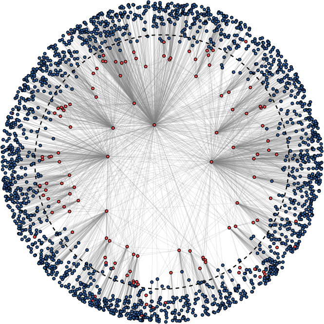
Figure 1: A hyperbolic random graph with $1942$ vertices, average degree $7.7$, and power-law exponent $2.6$. The vertex sets $V_{\text{Greedy}}$ and $V_{\text{Exact}}$ are shown in red and blue, respectively. The dashed line shows a possible threshold radius $\rho$.

To bound the size of $V_{\text{Greedy}}$, we identify a time during the execution of the algorithm at which only few vertices were added greedily, yet, the majority of the vertices were contained in small separated components (and were, therefore, part of $V_{\text{Exact}}$), and only few vertices remain to be added greedily. Since the algorithm processes the vertices by increasing radius, this point in time can be translated to a threshold radius $\rho$ in the hyperbolic disk (see Figure 1). Therefore, we divide the hyperbolic disk into two regions: an inner disk and an outer band, containing vertices with radii below and above $\rho$, respectively. The threshold $\rho$ is chosen such that a hyperbolic random graph decomposes into small components after removing the inner disk. When adding the first vertex from the outer band, greedily, we can assume that the inner disk is empty (since vertices of smaller radii were chosen before or removed as part of a small component). At this point, the majority of the vertices in the outer band were contained in small components, which have been solved exactly. In our analysis, we now overestimate the size of $V_{\text{Greedy}}$ by assuming that all remaining vertices are also added to the cover greedily. Therefore, we obtain a valid upper bound on $|V_{\text{Greedy}}|$, by counting the total number of vertices in the inner disk and adding the number of vertices in the outer band that are contained in components that are not solved exactly, i.e., components whose size exceeds $\tau\log\log(n)$. In the following, we show that both numbers are sublinear in $n$ with high probability. Together with the fact that an optimal vertex cover on hyperbolic random graphs, asymptotically almost surely, contains $\Omega(n)$ vertices [11], this implies $|V_{\text{Greedy}}|\in o(|C_{\text{OPT}}|)$.

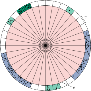
Figure 2: The disk is divided into the inner disk (red) and the outer band. It is additionally divided into sectors of equal width $\gamma$. Consecutive non-empty sectors form a run. Wide runs (blue) consist of many sectors. Each blue sector is a widening sector. Narrow runs (green) consist of few sectors. Small narrow runs contain only few vertices (light green), while large narrow runs contain many vertices (dark green).

The main contribution of our analysis is the identification of small components in the outer band, which is done by discretizing it into sectors, such that an edge cannot extend beyond an empty sector (see Figure 2). The foundation of this analysis is the delicate interplay between the angular width $\gamma$ of these sectors and the threshold $\rho$ that defines the outer band. Recall that $\rho$ is used to represent the time in the execution of the algorithm at which the graph has been decomposed into small components. For our analysis we assume that all vertices seen before this point (all vertices in the inner disk; red Figure 2) were added greedily. Therefore, if we choose $\rho$ too large, we overestimate the actual number of greedily added vertices by too much. As a consequence, we want to choose $\rho$ as small as possible. However, this conflicts our intentions for the choice of $\gamma$ and its impact on $\rho$. Recall that the maximum angular distance between two vertices such that they are adjacent increases with decreasing radii (Section 2). Thus, in order to avoid edges that extend beyond an angular width of $\gamma$, we need to ensure that the radii of the vertices in the outer band are sufficiently large. That is, decreasing $\gamma$ requires increasing $\rho$. However, we want to make $\gamma$ as small as possible, in order to get a finer granularity in the discretization and, with that, a more accurate analysis of the component structure in the outer band. Therefore, $\gamma$ and $\rho$ need to be chosen such that the inner disk does not become too large, while ensuring that the discretization is granular enough to accurately detect components whose size depends on $\tau$ and $n$. To this end, we adjust the angular width of the sectors using a function $\gamma(n,\tau)$, which is defined as

$$\gamma(n,\tau)=\log\left(\frac{\tau\log^{(2)}(n)}{2\log^{(3)}(n)^{2}}\right),$$

where $\log^{(i)}(n)$ denotes iteratively applying the $\log$-function $i$ times on $n$ (e.g., $\log^{(2)}(n)=\log\log(n)$), and set

$$\rho=R-\log(\pi/2\cdot e^{C/2}\gamma(n,\tau)),$$

where $R=2\log(n)+C$ is the radius of the hyperbolic disk.

In the following, we first show that the number of vertices in the inner disk is sublinear with high probability, before analyzing the component structure in the outer band. To this end, we make use of the discretization of the disk into sectors, by distinguishing between different kinds of runs (sequences of non-empty sectors), see Figure 2. In particular, we bound the number of wide runs (consisting of many sectors) and the number of vertices in them. Then we bound the number of vertices in large narrow runs (consisting of few sectors but containing many vertices). The remaining small narrow runs represent small components that are solved exactly.

The analysis mainly involves working with the random variables that denote the numbers of vertices in the above mentioned areas of the disk. Throughout the paper, we usually start with computing their expected values. Afterwards, we obtain tight concentration bounds using the previously mentioned Chernoff bound or, when the considered random variables are more involved, the method of (typical) bounded differences.

4.1 The Inner Disk

The inner disk $\mathcal{I}$ contains all vertices whose radius is below the threshold $\rho$. The number of them that are added to the cover greedily is bounded by the number of all vertices in $\mathcal{I}$.

Lemma 4.1.

Let $G$ be a hyperbolic random graph on $n$ vertices with power-law exponent $\beta=2\alpha+1$. With high probability, the number of vertices in $\mathcal{I}$ is in $\mathcal{O}(n\cdot\gamma(n,\tau)^{-\alpha})$.

Proof 4.2.

We start by computing the expected number of vertices in $\mathcal{I}$ and show concentration afterwards. To this end, we first compute the measure $\mu(\mathcal{I})$. The measure of a disk of radius $r$ that is centered at the origin is given by $e^{-\alpha(R-r)}(1+o(1))$ [20, Lemma 3.2]. Consequently, the expected number of vertices in $\mathcal{I}$ is

$$\mathbb{E}[|V(\mathcal{I})|] =n\mu(\mathcal{I})$$

$$=\mathcal{O}(ne^{-\alpha(R-\rho)})$$

$$=\mathcal{O}(ne^{-\alpha\log(\pi/2\,\cdot\,e^{C/2}\gamma(n,\tau))})$$

$$=\mathcal{O}\left(n\cdot\gamma(n,\tau)^{-\alpha}\right).$$

Since $\gamma(n,\tau)=\mathcal{O}(\log^{(3)}(n))$, this bound on $\mathbb{E}[|V(\mathcal{I})|]$ is $\omega(\log(n))$, and we can apply the Chernoff bound in Corollary 2.4 to conclude that $|V(\mathcal{I})|=\mathcal{O}\left(n\cdot\gamma(n,\tau)^{-\alpha}\right)$ holds with probability $1-\mathcal{O}(n^{-c})$ for any $c>0$.

Since $\gamma(n,\tau)=\omega(1)$, Lemma 4.1 shows that, with high probability, the number of vertices that are greedily added to the vertex cover in the inner disk is sublinear. Once the inner disk has been processed and removed, the graph has been decomposed into small components and the ones of size at most $\tau\log\log(n)$ have already been solved exactly. The remaining vertices that are now added greedily belong to large components in the outer band.

4.2 The Outer Band

To identify the vertices in the outer band that are contained in components whose size exceeds $\tau\log\log(n)$, we divide it into sectors of angular width $\gamma=\theta(\rho,\rho)=\pi\cdot\gamma(n,\tau)/n\cdot(1+o(1))$, where $\theta(\rho,\rho)$ denotes the maximum angular distance between two vertices with radii $\rho$ to be adjacent (see Section 2). This division is depicted in Figure 2. The choice of $\gamma$ (combined with the choice of $\rho$) has the effect that an edge between two vertices in the outer band cannot extend beyond an empty sector, i.e., a sector that does not contain any vertices, allowing us to use empty sectors as delimiters between components. To this end, we introduce the notion of runs, which are maximal sequences of non-empty sectors (see Figure 2). While a run can contain multiple components, the number of vertices in it denotes an upper bound on the combined sizes of the components that it contains.

To show that there are only few vertices in components whose size exceeds $\tau\log\log(n)$, we bound the number of vertices in runs that contain more than $\tau\log\log(n)$ vertices. For a given run this can happen for two reasons. First, it may contain many vertices if its angular interval is too large, i.e., it consists of too many sectors. This is unlikely, since the sectors are chosen sufficiently small, such that the probability for a given one to be empty is high. Second, while the angular width of the run is not too large, it contains too many vertices for its size. However, the vertices of the graph are distributed uniformly at random in the disk, making it unlikely that too many vertices are sampled into such a small area. To formalize this, we introduce a threshold $w$ and distinguish between two types of runs: A wide run contains more than $w$ sectors, while a narrow run contains at most $w$ sectors. The threshold $w$ is chosen such that the probabilities for a run to be wide and for a narrow run to contain more than $\tau\log\log(n)$ vertices are small. To this end, we set $w=e^{\gamma(n,\tau)}\cdot\log^{(3)}(n)$.

In the following, we first bound the number of vertices in wide runs. Afterwards, we consider narrow runs that contain more than $\tau\log\log(n)$ vertices. Together, this gives an upper bound on the number of vertices that are added greedily in the outer band.

4.2.1 Wide Runs

We refer to a sector that contributes to a wide run as a widening sector. In the following, we bound the number of vertices in all wide runs in three steps. First, we determine the expected number of all widening sectors. Second, based on the expected value, we show that the number of widening sectors is small, with high probability. Finally, we make use of the fact that the area of the disk covered by widening sectors is small, to show that the number of vertices sampled into the corresponding area is sublinear, with high probability.

Expected Number of Widening Sectors.

Let $n^{\prime}$ denote the total number of sectors and let $\mathcal{S}_{1},\dots,\mathcal{S}_{n^{\prime}}$ be the corresponding sequence. For each sector $\mathcal{S}_{k}$, we define the random variable $S_{k}$ indicating whether $\mathcal{S}_{k}$ contains any vertices, i.e., $S_{k}=0$ if $\mathcal{S}_{k}$ is empty and $S_{k}=1$ otherwise. The sectors in the disk are then represented by a circular sequence of indicator random variables $S_{1},\dots,S_{n^{\prime}}$, and we are interested in the random variable $W$ that denotes the sum of all runs of $1$s that are longer than $w$. In order to compute $\mathbb{E}[W]$, we first compute the total number of sectors, as well as the probability for a sector to be empty or non-empty.

Lemma 4.3.

Let $G$ be a hyperbolic random graph on $n$ vertices. Then, the number of sectors of width $\gamma=\theta(\rho,\rho)$ is $n^{\prime}=2n/\gamma(n,\tau)\cdot(1\pm o(1))$.

Proof 4.4.

Since all sectors have equal angular width $\gamma=\theta(\rho,\rho)$, we can use Section 2 to compute the total number of sectors as

$$n^{\prime} =2\pi/\theta(\rho,\rho)$$

$$=\pi e^{-R/2+\rho}(1\pm\Theta(e^{R-2\rho}))^{-1}.$$

By substituting $\rho=R-\log(\pi/2\cdot e^{C/2}\gamma(n,\tau))$ and $R=2\log(n)+C$, we obtain

$$n^{\prime} =\frac{\pi e^{R/2}}{\pi/2\cdot e^{C/2}\gamma(n,\tau)}(1\pm\Theta(e^{-R}\gamma(n,\tau)^{2}))^{-1}$$

$$=2n/\gamma(n,\tau)\cdot(1\pm\Theta((\gamma(n,\tau)/n)^{2}))^{-1}.$$

It remains to simplify the error term. Note that $\gamma(n,\tau)=\mathcal{O}(\log^{(3)}(n))$. Consequently, the error term is equivalent to $(1\pm o(1))^{-1}$. Finally, it holds that $1/(1+x)=1-\Theta(x)$ for $x=\pm o(1)$.

Lemma 4.5.

Let $G$ be a hyperbolic random graph on $n$ vertices and let $\mathcal{S}$ be a sector of angular width $\gamma=\theta(\rho,\rho)$. For sufficiently large $n$, the probability that $\mathcal{S}$ contains at least one vertex is bounded by

$$1-e^{-\gamma(n,\tau)/4}\leq\Pr[V(\mathcal{S})\neq\emptyset]\leq e^{-\left(e^{-\gamma(n,\tau)}\right)}.$$

Proof 4.6.

To compute the probability that $\mathcal{S}$ contains at least one vertex, we first compute the probability for a given vertex to fall into $\mathcal{S}$, which is given by the measure $\mu(\mathcal{S})$. Since the angular coordinates of the vertices are distributed uniformly at random and since the disk is divided into $n^{\prime}$ sectors of equal width, the measure of a single sector $\mathcal{S}$ can be obtained as $\mu(\mathcal{S})=1/n^{\prime}$. The total number of sectors $n^{\prime}$ is given by Lemma 4.3 and we can derive

$$\mu(\mathcal{S}) =\frac{\gamma(n,\tau)}{2n}(1\pm o(1))^{-1}=\frac{\gamma(n,\tau)}{2n}(1\pm o(1)),$$

where the second equality is obtained by applying $1/(1+x)=1-\Theta(x)$ for $x=\pm o(1)$.

Given $\mu(\mathcal{S})$, we first compute the lower bound on the probability that $\mathcal{S}$ contains at least one vertex. Note that $\Pr[V(\mathcal{S})\neq\emptyset]=1-\Pr[V(\mathcal{S})=\emptyset]$. Therefore, it suffices to show that $\Pr[V(\mathcal{S})=\emptyset]\leq e^{-\gamma(n,\tau)/4}$. The probability that $\mathcal{S}$ is empty is $(1-\mu(\mathcal{S}))^{n}$. Now recall that $1-x\leq e^{-x}$ for all $x\in\mathbb{R}$. Consequently, we have

$$\Pr[V(\mathcal{S})=\emptyset]\leq e^{-n\mu(\mathcal{S})}\leq e^{-\gamma(n,\tau)/2\,\cdot\,(1-o(1))}$$

and for large enough $n$ it holds that $1-o(1)\geq 1/2$.

It remains to compute the upper bound. Again, since $\Pr[V(\mathcal{S})\neq\emptyset]=1-\Pr[V(\mathcal{S})=\emptyset]$ and since $\Pr[V(\mathcal{S})=\emptyset]=(1-\mu(\mathcal{S}))^{n}$, we can compute the probability that $\mathcal{S}$ contains at least one vertex as

$$\Pr[V(\mathcal{S})\neq\emptyset]=1-(1-\mu(\mathcal{S}))^{n}.$$

Note that $\mu(\mathcal{S})\in o(1)$. Therefore, we can bound $1-x\geq e^{-x(1+o(1))}$ for $x\in o(1)$, and obtain the following bound on $\Pr[V(\mathcal{S})\neq\emptyset]$

$$\Pr[V(\mathcal{S})\neq\emptyset] =1-(1-\mu(\mathcal{S}))^{n}$$

$$\leq 1-e^{-n\mu(\mathcal{S})(1+o(1))}$$

$$\leq 1-e^{-\gamma(n,\tau)/2\,\cdot\,(1+o(1))}.$$

For large enough $n$, we have $(1+o(1))\leq 2$. Therefore,

$$\Pr[V(\mathcal{S})\neq\emptyset] \leq 1-e^{-\gamma(n,\tau)}$$

holds for sufficiently large $n$. Finally, $1-x\leq e^{-x}$ is valid for all $x\in\mathbb{R}$ and we obtain the claimed bound.

We are now ready to bound the expected number of widening sectors, i.e., sectors that are part of wide runs. To this end, we aim to apply the following lemma.

Lemma 4.7 ([30, Proposition 4.3]).

Let $S_{1},\dots,S_{n^{\prime}}$ denote a circular sequence of independent indicator random variables, such that $\Pr[S_{k}=1]=p$ and $\Pr[S_{k}=0]=1-p=q$, for all $k\in[n^{\prime}]$. Furthermore, let $W$ denote the sum of the lengths of all success runs of length at least $w\leq n^{\prime}$. Then, $\mathbb{E}[W]=n^{\prime}p^{w}(wq+p)$.

We note that the indicator random variables $S_{1},\dots,S_{n}^{\prime}$ are not independent on hyperbolic random graphs. To overcome this issue, we compute the expected value of $W$ on hyperbolic random graphs with $n$ vertices in expectation (see Section 2) and subsequently derive a probabilistic bound on $W$ for hyperbolic random graphs.

Lemma 4.8.

Let $G$ be a hyperbolic random graph with $n$ vertices in expectation and let $W$ denote the number of widening sectors. Then,

$$\mathbb{E}[W]\leq\frac{2^{1/4}\cdot\tau^{3/4}\cdot n}{\gamma(n,\tau)\cdot\log^{(2)}(n)^{1/4}\cdot\log^{(3)}(n)^{1/2}}(1\pm o(1)).$$

Proof 4.9.

A widening sector is part of a run of more than $w=e^{\gamma(n,\tau)}\cdot\log^{(3)}(n)$ consecutive non-empty sectors. To compute the expected number of widening sectors, we apply Lemma 4.7. To this end, we use Lemma 4.3 to bound the total number of sectors $n^{\prime}$ and bound the probability $p=\Pr[S_{k}=1]$ (i.e., the probability that sector $\mathcal{S}_{k}$ is not empty) as $p\leq\exp(-(e^{-\gamma(n,\tau)}))$, as well as the complementary probability $q=1-p\leq e^{-\gamma(n,\tau)/4}$, using Lemma 4.5. We obtain

$$\mathbb{E}[W] =n^{\prime}p^{(w+1)}((w+1)q+p)$$

$$\leq\frac{2n}{\gamma(n,\tau)}(1\pm o(1))\cdot e^{-\left((w+1)e^{-\gamma(n,\tau)}\right)}\cdot\left((w+1)e^{-\frac{\gamma(n,\tau)}{4}}+1\right)$$

$$\leq\frac{2n}{\gamma(n,\tau)}e^{\left(-e^{\gamma(n,\tau)}\log^{(3)}(n)e^{-\gamma(n,\tau)}\right)}$$

$$\hphantom{\leq\frac{2n}{\gamma(n,\tau)}\leavevmode\nobreak\ }\cdot\left((e^{\gamma(n,\tau)}\log^{(3)}(n)+1)e^{-\frac{\gamma(n,\tau)}{4}}+1\right)(1\pm o(1)).$$

Now the first exponential simplifies to $\exp(-\log^{(3)}(n))=\log^{(2)}(n)^{-1}$, since the $\gamma(n,\tau)$ terms cancel. Factoring out $\exp(3/4\cdot\gamma(n,\tau))\log^{(3)}(n)$ in the third term then yields

$$\mathbb{E}[W] \leq\frac{2ne^{3/4\,\cdot\,\gamma(n,\tau)}\log^{(3)}(n)}{\gamma(n,\tau)\cdot\log^{(2)}(n)}$$

$$\qquad\cdot\left(1+\frac{1}{e^{\gamma(n,\tau)}\log^{(3)}(n)}+\frac{1}{e^{3/4\,\cdot\,\gamma(n,\tau)}\log^{(3)}(n)}\right)(1\pm o(1)).$$

Since $\gamma(n,\tau)=\omega(1)$, the first error term can be simplified as $(1+o(1))$. Additionally, we can substitute $\gamma(n,\tau)=\log(\tau\log^{(2)}(n)/(2\log^{(3)}(n)^{2}))$ to obtain

$$\mathbb{E}[W] \leq 2^{1/4}\frac{\tau^{3/4}\cdot n\cdot\log^{(3)}(n)}{\gamma(n,\tau)\cdot\log^{(2)}(n)}\cdot\frac{\log^{(2)}(n)^{3/4}}{\log^{(3)}(n)^{3/2}}\cdot(1\pm o(1)).$$

Further simplification then yields the claim.

Concentration Bound on the Number of Widening Sectors.

Lemma 4.8 bounds the expected number of widening sectors and it remains to show that this bound holds with high probability. To this end, we first determine under which conditions the sum of long success runs in a circular sequence of indicator random variables can be bounded with high probability in general. Afterwards, we show that these conditions are met for our application.

Lemma 4.10.

Let $S_{1},\dots,S_{n^{\prime}}$ denote a circular sequence of independent indicator random variables and let $W$ denote the sum of the lengths of all success runs of length at least $1\leq w\leq n^{\prime}$. If $g(n^{\prime})=\omega(w\sqrt{n^{\prime}\log(n^{\prime})})$ is an upper bound on $\mathbb{E}[W]$, then $W=\mathcal{O}(g(n^{\prime}))$ holds with probability $1-\mathcal{O}((n^{\prime})^{-c})$ for any constant $c$.

Proof 4.11.

In order to show that $W$ does not exceed $g(n^{\prime})$ by more than a constant factor with high probability, we aim to apply a method of bounded differences (Corollary 2.7). To this end, we consider $W$ as a function of $n^{\prime}$ independent random variables $S_{1},\dots,S_{n^{\prime}}$ and determine the parameters $\Delta_{i}$ with which $W$ satisfies the bounded differences condition (see Equation 3). That is, for each $i\in[n^{\prime}]$ we need to bound the change in the sum of the lengths of all success runs of length at least $w$, obtained by changing the value of $S_{i}$ from $0$ to $1$ or vice versa.

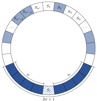
Figure 3: A circular sequence of random variables $S_{1},\dots,S_{n^{\prime}}$ that can either be $0$ (white) or $1$ (blue). Dark blue runs are as large as possible without being wide. Depending on the value of $S_{i}$, the two runs of length $w$ are merged into one run of length $2w+1$.

The largest impact on $W$ is obtained when changing the value of $S_{i}$ from $0$ to $1$ merges two runs of size $w$, i.e., runs that are as large as possible but not wide, as shown in Figure 3. In this case both runs did not contribute anything to $W$ before the change, while the merged run now contributes $2w+1$. Then, we can bound the change in $W$ as $\Delta_{i}=2w+1$. Note that the other case in which the value of $S_{i}$ is changed from $1$ to $0$ can be viewed as the inversion of the change in the first case. That is, instead of merging two runs, changing $S_{i}$ splits a single run into two. Consequently, the corresponding bound on the change of $W$ is the same, except that $W$ is decreasing instead of increasing.

It follows that $W$ satisfies the bounded differences condition for $\Delta_{i}=2w+1$ for all $i\in\{1,\dots,n^{\prime}\}$. We can now apply Corollary 2.7 to bound the probability that $W$ exceeds an upper bound $g(n^{\prime})$ on its expected value by more than a constant factor as

$$\Pr[W>c_{1}g(n^{\prime})]\leq e^{-2((c_{1}-1)g(n^{\prime}))^{2}/\Delta},$$

where $\Delta=\sum_{i}\Delta_{i}^{2}$ and $c_{1}\geq 1$. Since $\Delta_{i}=2w+1$ for all $i\in[n^{\prime}]$, we have $\Delta=n^{\prime}(2w+1)^{2}$. Thus,

$$\Pr[W>c_{1}g(n^{\prime})]\leq e^{-\frac{2((c_{1}-1)g(n^{\prime}))^{2}}{n^{\prime}(2w+1)^{2}}}\leq e^{-\frac{2(c_{1}-1)^{2}}{n^{\prime}}\,\cdot\,\left(\frac{g(n^{\prime})}{3w}\right)^{2}},$$

where the second inequality is valid since $w$ is assumed to be at least $1$. Moreover, we can apply $g(n^{\prime})=\omega(w\sqrt{n^{\prime}\log(n^{\prime})})$ (a precondition of this lemma), which yields

$$\Pr[W>c_{1}g(n^{\prime})]=(n^{\prime})^{-\omega(1)}.$$

Therefore, it holds that $\Pr[W\in\mathcal{O}(g(n^{\prime}))]=1-(n^{\prime})^{-\omega(1)}=1-\mathcal{O}((n^{\prime})^{-c})$ for any constant $c$.

Lemma 4.12.

Let $G$ be a hyperbolic random graph on $n$ vertices. Then, with probability $1-\mathcal{O}(n^{-c})$ for any constant $c>0$, the number of widening sectors is

$$W=\mathcal{O}\left(\frac{\tau^{3/4}\cdot n}{\gamma(n,\tau)\cdot\log^{(2)}(n)^{1/4}\cdot\log^{(3)}(n)^{1/2}}\right).$$

Proof 4.13.

In the following, we show that the claimed bound holds with probability $1-\mathcal{O}(n^{-c_{1}})$ for any constant $c_{1}>0$ on hyperbolic random graphs with $n$ vertices in expectation. By Lemma 2.1 the same bound then holds with probability $1-\mathcal{O}(n^{-c_{1}+1/2})$ on hyperbolic random graphs. Choosing $c=c_{1}-1/2$ then yields the claim.

Recall that we represent the sectors using a circular sequence of independent indicator random variables $S_{1},\dots,S_{n^{\prime}}$ and that $W$ denotes the sum of the lengths of all success runs spanning more than $w$ sectors, i.e., the sum of all widening sectors. By Lemma 4.8 we obtain a valid upper bound on $\mathbb{E}[W]$ by choosing

$$g(n^{\prime})=h(n)=\frac{2^{1/4}\cdot\tau^{3/4}\cdot n}{\gamma(n,\tau)\cdot\log^{(2)}(n)^{1/4}\cdot\log^{(3)}(n)^{1/2}}(1\pm o(1))$$

and it remains to show that this bound holds with sufficiently high probability. To this end, we aim to apply Lemma 4.10, which states that $W=\mathcal{O}(g(n^{\prime}))$ holds with probability $1-\mathcal{O}((n^{\prime})^{-c_{2}})$ for any constant $c_{2}$, if $g(n^{\prime})=\omega(w\sqrt{n^{\prime}\log(n^{\prime})})$. In the following, we first show that $h(n)$ fulfills this criterion, before arguing that we can choose $c_{2}$ such that $1-\mathcal{O}((n^{\prime})^{-c_{2}})=1-\mathcal{O}(n^{-c_{1}})$ for any constant $c_{1}$.

Since $\tau$ is constant and $n^{\prime}=2n/\gamma(n,\tau)\cdot(1\pm o(1))$ by Lemma 4.3, we can bound $h(n)$ by

$$h(n) =\Theta\left(\frac{n^{\prime}}{\log^{(2)}(n)^{1/4}\log^{(3)}(n)^{1/2}}\right)$$

$$=\Theta\left(\frac{\log^{(2)}(n)\cdot n^{\prime}}{\log^{(2)}(n)^{5/4}\log^{(3)}(n)^{1/2}}\right)$$

$$=\omega\left(\frac{\log^{(2)}(n)}{\log^{(3)}(n)}\cdot\frac{n^{\prime}}{\log^{(2)}(n)^{5/4}}\right),$$

where the last bound is obtained by applying $\log^{(3)}(n)^{1/2}=\omega(1)$. Recall that $w$ was chosen as $w=e^{\gamma(n,\tau)}\log^{(3)}(n)$. Furthermore, we have $\gamma(n,\tau)=\log(\tau\log^{(2)}(n)/(2\log^{(3)}(n)^{2}))$. Thus, it holds that $w=\Theta(\log^{(2)}(n)/(\log^{(3)}(n)))$, allowing us to further bound $h(n)$ by

$$h(n) =\omega\left(w\frac{n^{\prime}}{\log^{(2)}(n)^{5/4}}\right)$$

$$=\omega\left(w\sqrt{n^{\prime}\log(n^{\prime})\cdot\frac{n^{\prime}}{\log(n^{\prime})\log^{(2)}(n)^{5/2}}}\right)$$

and it remains to show that the last factor in the root is in $\omega(1)$. Note that $n^{\prime}=\Omega(n/\log^{(3)}(n))$ and $n^{\prime}=\mathcal{O}(n)$. Consequently, it holds that

$$\frac{n^{\prime}}{\log(n^{\prime})\log^{(2)}(n)^{5/2}} =\Omega\left(\frac{n}{\log(n)\cdot\log^{(2)}(n)^{5/2}\cdot\log^{(3)}(n)}\right)=\omega\left(\frac{n}{\log(n)^{3}}\right)=\omega(1).$$

As stated above, this shows that $W=\mathcal{O}(h(n))$ holds with probability $1-\mathcal{O}((n^{\prime})^{-c_{2}})$ for any constant $c_{2}$. Again, since $n^{\prime}=\Omega(n/\log^{(3)}(n))$, we have $n^{\prime}=\Omega(n^{1/2})$. Therefore, we can conclude that $W=\mathcal{O}(h(n))$ holds with probability $1-\mathcal{O}(n^{-c_{2}/2})$. Choosing $c_{2}=2c_{1}$ then yields the claim.

Number of Vertices in Wide Runs.

Let $\mathcal{W}$ denote the area of the disk covered by all widening sectors. By Lemma 4.12 the total number of widening sectors is small, with high probability. As a consequence, $\mathcal{W}$ is small as well and we can derive that the size of the vertex set $V(\mathcal{W})$ containing all vertices in all widening sectors is sublinear with high probability.

Lemma 4.14.

Let $G$ be a hyperbolic random graph on $n$ vertices. Then, with high probability, the number of vertices in wide runs is bounded by

$$|V(\mathcal{W})|=\mathcal{O}\left(\frac{\tau^{3/4}\cdot n}{\log^{(2)}(n)^{1/4}\cdot\log^{(3)}(n)^{1/2}}\right).$$

Proof 4.15.

We start by computing the expected number of vertices in $\mathcal{W}$ and show concentration afterwards. The probability for a given vertex to fall into $\mathcal{W}$ is equal to its measure $\mu(\mathcal{W})$. Since the angular coordinates of the vertices are distributed uniformly at random, we have $\mu(\mathcal{W})=W/n^{\prime}$, where $W$ denotes the number of widening sectors and $n^{\prime}$ is the total number of sectors, which is given by Lemma 4.3. The expected number of vertices in $\mathcal{W}$ is then

$$\mathbb{E}[|V(\mathcal{W})|]=n\mu(\mathcal{W})=n\frac{W}{n^{\prime}}=\frac{1}{2}W\cdot\gamma(n,\tau)(1\pm o(1)),$$ (5)

where the last equality holds since $1/(1+x)=1-\Theta(x)$ is valid for $x=\pm o(1)$. Note that the number of widening sectors $W$ is itself a random variable. Therefore, we apply the law of total expectation and consider different outcomes of $W$ weighted with their probabilities. Motivated by the previously determined probabilistic bound on $W$ (Lemma 4.12), we consider the events $W\leq g(n)$ as well as $W>g(n)$, where

$$g(n)=\frac{c\cdot\tau^{3/4}\cdot n}{\gamma(n,\tau)\cdot\log^{(2)}(n)^{1/4}\cdot\log^{(3)}(n)^{1/2}},$$

for sufficiently large $c>0$ and $n$. With this, we can compute the expected number of vertices in $\mathcal{W}$ as

$$\mathbb{E}[|V(\mathcal{W})|]=\leavevmode\nobreak\ \mathbb{E}[|V(\mathcal{W})|\mid W\leq g(n)]\cdot\Pr[W\leq g(n)]\leavevmode\nobreak\ +$$

$$\mathbb{E}[|V(\mathcal{W})|\mid W>g(n)]\cdot\Pr[W>g(n)].$$

To bound the first summand, note that $\Pr[W\leq g(n)]\leq 1$. Further, by applying Equation 5 from above, we have

$$\mathbb{E}[|V(\mathcal{W})|\mid W\leq g(n)]\cdot\Pr[W\leq g(n)] \leq\frac{1}{2}g(n)\cdot\gamma(n,\tau)(1\pm o(1)).$$

In order to bound the second summand, note that $n$ is an obvious upper bound on $\mathbb{E}[|V(\mathcal{W})|]$. Moreover, by Lemma 4.12 it holds that $\Pr[W>g(n)]=\mathcal{O}(n^{-c_{1}})$ for any $c_{1}>0$. As a result we have

$$\mathbb{E}[|V(\mathcal{W})|\mid W>g(n)]\cdot\Pr[W>g(n)]\leq n\Pr[W>g(n)] =\mathcal{O}(n^{-c_{1}+1}),$$

for any $c_{1}>0$. Clearly, the first summand dominates the second and we can conclude that $\mathbb{E}[|V(\mathcal{W})|]=\mathcal{O}(g(n)\gamma(n,\tau))$. Consequently, for large enough $n$, there exists a constant $c_{2}>0$ such that $\hat{g}(n)=c_{2}g(n)\gamma(n,\tau)$ is a valid upper bound on $\mathbb{E}[|V(\mathcal{W})|]$. This allows us to apply the Chernoff bound in Corollary 2.4 to bound the probability that $|V(\mathcal{W})|$ exceeds $\hat{g}(n)$ by more than a constant factor as

$$\Pr[|V(\mathcal{W})|\geq(1+\varepsilon)\hat{g}(n)]\leq e^{-\varepsilon^{2}/3\,\cdot\,\hat{g}(n)}.$$

Finally, since $\hat{g}(n)$ can be simplified as

$$\hat{g}(n)=c_{2}\cdot\frac{c\cdot\tau^{3/4}\cdot n}{\log^{(2)}(n)^{1/4}\cdot\log^{(3)}(n)^{1/2}},$$

it is easy to see that $\hat{g}(n)=\omega(\log(n))$ and thus $|V(\mathcal{W})|=\mathcal{O}(\hat{g}(n))$ holds with probability $1-\mathcal{O}(n^{-c_{3}})$ for any $c_{3}>0$.

It remains to bound the number of vertices in large components contained in narrow runs.

4.2.2 Narrow Runs

In the following, we differentiate between small and large narrow runs, containing at most and more than $\tau\log^{(2)}(n)$ vertices, respectively. As before, we first bound the expected number of vertices in all large narrow runs and deal with concentration afterwards.

Expected Number of Vertices in Large Narrow Runs.

The straight-forward way to bounding the number of vertices in all large narrow runs is to consider each sector and count the contained number of vertices, if the sector is part of a large narrow run. Unfortunately, whether this is the case depends on the surrounding sectors and whether they are empty (ending the run) or contain lots of vertices (to make the run large), and dealing with these stochastic dependencies is difficult.

To relax these dependencies, we determine an upper bound on the number of vertices in large narrow runs, by not only considering sectors that are part of such a run, but also ones that are in the proximity thereof. More precisely, for a sector $\mathcal{S}$ we define its narrow proximity $\mathcal{P}_{\mathcal{S}}$ as $\mathcal{S}$ together with the $w-1$ sectors to its left and the $w-1$ sectors to its right. If $\mathcal{S}$ is part of a large narrow run, then there are more than $\tau\log^{(2)}(n)$ vertices in its narrow proximity. Note, however, that this condition is not sufficient: Even if there are as many vertices in $\mathcal{P}_{\mathcal{S}}$, there could be empty sectors that cut $\mathcal{S}$ off from the corresponding sectors, in which case $\mathcal{S}$ is not part of a large narrow run.

We start by bounding the expected number of vertices in the narrow proximity of a sector.

Lemma 4.16.

Let $G$ be a hyperbolic random graph on $n$ vertices, let $\mathcal{S}$ be a sector, and let $\mathcal{P}_{\mathcal{S}}$ be its narrow proximity. Then, $\mathbb{E}[|V(\mathcal{P}_{\mathcal{S}})|]\leq e^{\gamma(n,\tau)}\log^{(3)}(n)\gamma(n,\tau)(1\pm o(1))$.

Proof 4.17.

The narrow proximity of $\mathcal{S}$ consists of $\mathcal{S}$ together with the $w-1$ sectors to its left and the $w-1$ ones to its right. In particular, $\mathcal{P}(\mathcal{S})$ consists of at most $2w$ sectors. Since the angular coordinates of the vertices are distributed uniformly at random and since we partitioned the disk into $n^{\prime}$ disjoint sectors of equal width, we can derive an upper bound on the expected number of vertices in $\mathcal{P}_{\mathcal{S}}$ as $\mathbb{E}[|V(\mathcal{P}_{\mathcal{S}})|]\leq n\cdot 2w/n^{\prime}$. As $w=e^{\gamma(n,\tau)}\log^{(3)}(n)$ by definition and $n^{\prime}=2n/\gamma(n,\tau)\cdot(1\pm o(1))$ according to Lemma 4.3, we have

$$\mathbb{E}[|V(\mathcal{P}_{\mathcal{S}})|]\leq e^{\gamma(n,\tau)}\log^{(3)}(n)\gamma(n,\tau)(1\pm o(1))^{-1}.$$

Since $1/(1+x)=1-\Theta(x)$ for $x=\pm o(1)$, we obtain the claimed bound.

Using this upper bound, we can bound the probability that the number of vertices in the narrow proximity of a sector exceeds the threshold $\tau\log^{(2)}(n)$ by a certain amount.

Lemma 4.18.

Let $G$ be a hyperbolic random graph on $n$ vertices, let $\mathcal{S}$ be a sector, and let $\mathcal{P}_{\mathcal{S}}$ be its narrow proximity. For $k>\tau\log^{(2)}(n)$ and $n$ large enough, it holds that $\Pr[|V(\mathcal{P}_{\mathcal{S}})|=k]\leq e^{-k/18}$.

Proof 4.19.

First note that $\Pr[|V(\mathcal{P}_{\mathcal{S}})|=k]\leq\Pr[|V(\mathcal{P}_{\mathcal{S}})|\geq k]$. In order to show that $\Pr[|V(\mathcal{P}_{\mathcal{S}})|\geq k]$ is small, we aim to apply the Chernoff bound in Corollary 2.4, choosing $\varepsilon=1/2$ and $g(n)=2/3\cdot k$ as an upper bound on $\mathbb{E}[|V(\mathcal{P}_{\mathcal{S}})|]$. To see that this is a valid choice, we use Lemma 4.16 and substitute $\gamma(n,\tau)=\log(\tau\log^{(2)}(n)/(2\log^{(3)}(n)^{2}))$, which yields

$$\mathbb{E}[|V(\mathcal{P}_{\mathcal{S}})|] \leq e^{\gamma(n,\tau)}\log^{(3)}(n)\gamma(n,\tau)(1\pm o(1))$$

$$=\frac{\tau\log^{(2)}(n)}{2\log^{(3)}(n)^{2}}\cdot\log^{(3)}(n)\cdot\log\left(\frac{\tau\log^{(2)}(n)}{2\log^{(3)}(n)^{2}}\right)(1\pm o(1))$$

$$=\frac{\tau\log^{(2)}(n)}{2\log^{(3)}(n)}\cdot\left(\log^{(3)}(n)-\left(2\log^{(4)}(n)-\log(\tau/2)\right)\right)(1\pm o(1))$$

$$=\frac{1}{2}\cdot\tau\log^{(2)}(n)\cdot\left(1-\frac{2\log^{(4)}(n)-\log(\tau/2)}{\log^{(3)}(n)}\right)(1\pm o(1)).$$

Note, that the first error term is equivalent to $(1-o(1))$ and that $(1\pm o(1))\leq 4/3$ holds for $n$ large enough. Consequently, for sufficiently large $n$, we have $\mathbb{E}[|V(\mathcal{P}_{\mathcal{S}})|]\leq 2/3\cdot\tau\log^{(2)}(n)$. Since $k>\tau\log^{(2)}(n)$, it follows that $g(n)=2/3\cdot k$ is a valid upper bound on $\mathbb{E}[|V(\mathcal{P}_{\mathcal{S}})|]$. Therefore, we can apply the Chernoff bound in Corollary 2.4 to conclude that

$$\Pr[|V(\mathcal{P}_{\mathcal{S}})|\geq k] \leq e^{-(1/2)^{2}/3\,\cdot\,g(n)}=e^{-1/12\,\cdot\,2/3\,\cdot\,k}=e^{-k/18}.$$

We are now ready to bound the expected value of the number $N$ of vertices in all large narrow runs.

Lemma 4.20.

Let $G$ be a hyperbolic random graph. Then, the expected number of vertices in all large narrow runs is bounded by

$$\mathbb{E}[N]=\mathcal{O}\left(\frac{n\cdot\log^{(3)}(n)}{\gamma(n,\tau)\log(n)^{\tau/18}}\right).$$

Proof 4.21.

For the $i$-th sector $\mathcal{S}_{i}$ ($i\in[n^{\prime}]$) we define a random variable $N_{i}$, with $N_{i}=|V(\mathcal{S}_{i})|$ if $\mathcal{S}_{i}$ is part of a large narrow run and $N_{i}=0$ otherwise. Then $N=\sum_{i\in[n^{\prime}]}N_{i}$. As mentioned above, we compute an upper bound of $\mathbb{E}[N]$ by considering random variables $N_{i}^{\prime}$ instead, where $N_{i}^{\prime}=|V(\mathcal{S}_{i})|$ if the number of vertices in the narrow proximity of $\mathcal{S}_{i}$ exceeds the threshold $t=\tau\log^{(2)}(n)$, and $N_{i}^{\prime}=0$ otherwise. By the above argumentation it holds that $N_{i}^{\prime}\geq N_{i}$ and thus for $N^{\prime}=\sum_{i\in[n^{\prime}]}N_{i}^{\prime}$ we have $N^{\prime}\geq N$. Consequently, it suffices to show that the claimed bound holds for $\mathbb{E}[N^{\prime}]$. To this end, we compute

$$\mathbb{E}[N^{\prime}]=\sum_{i=1}^{n^{\prime}}\mathbb{E}[N_{i}^{\prime}]=\sum_{i=1}^{n^{\prime}}\sum_{k=0}^{n}\mathbb{E}\left[N_{i}\leavevmode\nobreak\ \big{|}\leavevmode\nobreak\ |V(\mathcal{P}_{\mathcal{S}_{i}})|=k\right]\cdot\Pr[|V(\mathcal{P}_{\mathcal{S}_{i}})|=k],$$

where the second equality is obtained using the law of total expectation. Note that we have $N_{i}^{\prime}=0$ whenever $|V(\mathcal{P}_{\mathcal{S}_{i}})|\leq t$, and $N_{i}=|V(\mathcal{S}_{i})|$, otherwise. Thus, the expression simplifies to

$$\mathbb{E}[N^{\prime}]=\sum_{i=1}^{n^{\prime}}\sum_{k=t+1}^{n}\mathbb{E}\left[|V(\mathcal{S}_{i})|\leavevmode\nobreak\ \big{|}\leavevmode\nobreak\ |V(\mathcal{P}_{\mathcal{S}_{i}})|=k\right]\cdot\Pr[|V(\mathcal{P}_{\mathcal{S}_{i}})|=k],$$

In each summand we are interested in the expected number of vertices in a sector $\mathcal{S}_{i}$, conditioned on the fact that its narrow proximity contains exactly $k$ vertices. Since the angular coordinates of the vertices are distributed uniformly and the narrow proximity consists of $2w-1$ sectors including $\mathcal{S}_{i}$, the expected number that end up in $\mathcal{S}_{i}$ is given by $k/(2w-1)\leq k/w$. It follows that

$$\mathbb{E}[N^{\prime}]\leq\sum_{i=1}^{n^{\prime}}\sum_{k=t+1}^{n}\frac{k}{w}\cdot\Pr[|V(\mathcal{P}_{\mathcal{S}_{i}})|=k].$$

The probability can be bounded using Lemma 4.18, which yields for $k>\tau\log^{(2)}(n)=t$ that $\Pr[|V(\mathcal{P}_{\mathcal{S}_{i}})|=k]\leq e^{-k/18}$. Thus,

$$\mathbb{E}[N^{\prime}]\leq\frac{n^{\prime}}{w}\sum_{k=t+1}^{n}k\cdot e^{-k/18}.$$

Note that the sum is of the form $\sum kb^{k}$ for $b=e^{-1/18}<1$, which is the derivative of the geometric series multiplied by $b$. Consequently, we obtain an upper bound by bounding the limits as $t+1>t$ and $n<\infty$ and applying the identity

$$\sum_{k=t}^{\infty}kb^{k}=\frac{b^{t}(t+b-tb)}{(b-1)^{2}},$$

which is valid for $b<1$ and reduces to $\mathcal{O}(b^{t}\cdot t)$ for constant $b$. Substituting $b=e^{-1/18}$ and $t=\tau\log^{(2)}(n)$ then yields

$$\mathbb{E}[N^{\prime}]\leq\frac{n^{\prime}}{w}\mathcal{O}\left(e^{-\tau\log^{(2)}(n)/18}\cdot\log^{(2)}(n)\right)=\mathcal{O}\left(\frac{n^{\prime}}{w}\frac{\log^{(2)}(n)}{\log(n)^{\tau/18}}\right).$$

Finally, since $w=e^{\gamma(n,\tau)}\log^{(3)}(n)$ by definition and $n^{\prime}=\mathcal{O}(n/\gamma(n,\tau))$ by Lemma 4.3, where we defined $\gamma(n,\tau)=\log(\tau\log^{(2)}(n)/(2\log^{(3)}(n)^{2}))$, the above term can be simplified to

$$\mathbb{E}[N^{\prime}] =\mathcal{O}\left(\frac{n}{\gamma(n,\tau)\cdot e^{\gamma(n,\tau)}\log^{(3)}(n)}\cdot\frac{\log^{(2)}(n)}{\log(n)^{\tau/18}}\right)$$

$$=\mathcal{O}\left(\frac{n}{\gamma(n,\tau)\cdot\frac{\log^{(2)}(n)}{\log^{(3)}(n)}}\cdot\frac{\log^{(2)}(n)}{\log(n)^{\tau/18}}\right)$$

$$=\mathcal{O}\left(\frac{n\cdot\log^{(3)}(n)}{\gamma(n,\tau)\cdot\log(n)^{\tau/18}}\right).$$

Concentration Bound on the Number of Vertices in Large Narrow Runs.

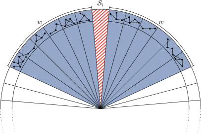
Figure 4: The random variable $S_{i}$ indicates whether $\mathcal{S}_{i}$ contains any vertices. Changing $S_{i}$ from $0$ to $1$ or vice versa merges two narrow runs or splits a wide run into two narrow ones, respectively. If all vertices were placed in the blue area, moving a single vertex in or out of $\mathcal{S}_{i}$ may change the number of vertices in large narrow runs by $n$.

To show that the actual number of vertices in large narrow runs $N$ is not much larger than the expected value, we consider $N$ as a function of $n$ independent random variables $P_{1},\dots,P_{n}$ representing the positions of the vertices in the hyperbolic disk. In order to show that $N$ does not deviate much from its expected value with high probability, we would like to apply the method of bounded differences, which builds on the fact that $N$ satisfies the bounded differences condition, i.e., that changing the position of a single vertex does not change $N$ by much. Unfortunately, this change is not small in general.

In the worst case, there is a wide run $\mathcal{R}$ that contains all vertices and a sector $\mathcal{S}_{i}\subseteq\mathcal{R}$ contains only one of them. Moving this vertex out of $\mathcal{S}_{i}$ may split the run into two narrow runs (see Figure 4). These still contain $n$ vertices, which corresponds to the change in $N$. However, this would mean that $\mathcal{R}$ consists of only few sectors (since it can be split into two narrow runs) and that all vertices lie within the corresponding (small) area of the disk. Since the vertices of the graph are distributed uniformly, this is very unlikely. To take advantage of this, we apply the method of typical bounded differences (Corollary 2.10), which allows us to milden the effects of the change in the unlikely worst case and to focus on the typically smaller change of $N$ instead. Formally, we represent the typical case using an event $A$ denoting that each run of length at most $2w+1$ contains at most $\mathcal{O}(\log(n))$ vertices. In the following, we show that $A$ occurs with probability $1-\mathcal{O}(n^{-c})$ for any constant $c$, which shows that the atypical case is very unlikely.

Lemma 4.22.

Let $G$ be a hyperbolic random graph. Then, each run of length at most $2w+1$ contains at most $\mathcal{O}(\log(n))$ vertices with probability $1-\mathcal{O}(n^{-c})$ for any constant $c$.

Proof 4.23.

We show that the probability for a single run $\mathcal{R}$ of at most $2w+1$ sectors to contain more then $\mathcal{O}(\log(n))$ vertices is $\mathcal{O}(n^{-c_{1}})$ for any constant $c_{1}$. Since there are at most $n^{\prime}=\mathcal{O}(n)$ runs, applying the union bound and choosing $c_{1}=c+1$ then yields the claim.

Recall that we divided the disk into $n^{\prime}$ sectors of equal width. Since the angular coordinates of the vertices are distributed uniformly at random, the probability for a given vertex to a lie in $\mathcal{R}$ (i.e., to be in $V(\mathcal{R})$) is given by

$$\mu(\mathcal{R})\leq\frac{2w+1}{n^{\prime}}=\frac{2e^{\gamma(n,\tau)}\log^{(3)}(n)+1}{n^{\prime}}.$$

By Lemma 4.3 the total number of sectors is given as $n^{\prime}=2n/\gamma(n,\tau)\cdot(1\pm o(1))$. Consequently, we can compute the expected number of vertices in $\mathcal{R}$ as

$$\mathbb{E}[|V(\mathcal{R})|]\leq n\mu(\mathcal{R})=\left(e^{\gamma(n,\tau)}\log^{(3)}(n)+1/2\right)\gamma(n,\tau)(1\pm o(1)).$$

Substituting $\gamma(n,\tau)=\mathcal{O}(\log(\log^{(2)}(n)/\log^{(3)}(n)^{2}))$, we can derive that

$$\mathbb{E}[|V(\mathcal{R})|]\leq\mathcal{O}\left(\frac{\log^{(2)}(n)}{\log^{(3)}(n)^{2}}\log^{(3)}(n)\cdot\log\left(\frac{\log^{(2)}(n)}{\log^{(3)}(n)^{2}}\right)\right)=\mathcal{O}(\log^{(2)}(n)).$$

Consequently, it holds that $g(n)=c_{2}\log(n)$ is a valid upper bound for any $c_{2}>0$ and large enough $n$. Therefore, we can apply the Chernoff bound in Corollary 2.4 to conclude that the probability for the number of vertices in $\mathcal{R}$ to exceed $g(n)$ is at most

$$\Pr[|V(\mathcal{R})|\geq(1+\varepsilon)g(n)]\leq e^{-\varepsilon^{2}/3\,\cdot\,g(n)}=n^{-c_{2}\varepsilon^{2}/3}.$$

Thus, $c_{2}$ can be chosen sufficiently large, such that

$$\Pr[|V(\mathcal{R})|\geq(1+\varepsilon)g(n)]=\mathcal{O}(n^{-c_{1}})$$

for any constant $c_{1}$.

The method of typical bounded differences now allows us to focus on this case and to milden the impact of the worst case changes as they occur with small probability. Consequently, we can show that the number of vertices in large narrow runs is sublinear with high probability.

Lemma 4.24.

Let $G$ be a hyperbolic random graph. Then, with high probability, the number of vertices in large narrow runs is bounded by

$$N=\mathcal{O}\left(\frac{n\cdot\log^{(3)}(n)}{\gamma(n,\tau)\log(n)^{\tau/18}}\right).$$

Proof 4.25.

Recall that the expected number of vertices in all large narrow runs is given by Lemma 4.20. Consequently, we can choose $c>0$ large enough, such that for sufficiently large $n$ we obtain a valid upper bound on $\mathbb{E}[N]$ by choosing

$$g(n)=\frac{c\cdot n\cdot\log^{(3)}(n)}{\gamma(n,\tau)\log(n)^{\tau/18}}.$$

In order to show that $N$ does not exceed $g(n)$ by more than a constant factor with high probability, we apply the method of typical bounded differences (Corollary 2.10). To this end, we consider the typical event $A$, denoting that each run of at most $2w+1$ sectors contains at most $\mathcal{O}(\log(n))$ vertices, and it remains to determine the parameters $\Delta_{i}^{A}\leq\Delta_{i}$ with which $N$ satisfies the typical bounded differences condition with respect to $A$ (see Equation 4). Formally, we have to show that for all $i\in\{1,\dots,n\}$

$$|N(P_{1},\dots,P_{i},\dots,P_{n})-N(P_{1},\dots,P_{i}^{\prime},\dots,P_{n})|\leq\begin{cases}\Delta_{i}^{A},\mkern-16.0mu&\text{if}\leavevmode\nobreak\ (P_{1},\dots,P_{i},\dots,P_{n})\in A,\\ \Delta_{i},\mkern-16.0mu&\text{otherwise}.\end{cases}$$

As argued before, changing the position $P_{i}$ of vertex $i$ to $P_{i}^{\prime}$ may result in a change of $n$ in the worst case. Therefore, $\Delta_{i}=n$ is a valid bound for all $i\in[n]$. To bound the $\Delta_{i}^{A}$, we have to consider the following situation. We start with a set of positions such that all runs of $2w+1$ sectors contain at most $\mathcal{O}(\log(n))$ vertices and we want to bound the change in $N$ when changing the position $P_{i}$ of a single vertex $i$. In this case, splitting a wide run or merging two narrow runs can only change $N$ by $\mathcal{O}(\log(n))$. Consequently, we can choose $\Delta_{i}^{A}=\mathcal{O}(\log(n))$ for all $i\in[n]$. By Corollary 2.10 we can now bound the probability that $N$ exceeds $g(n)$ by more than a constant factor $c_{1}$ as

$$\Pr[N>c_{1}g(n)]\leq e^{-((c_{1}-1)g(n))^{2}/(2\Delta)}+\Pr[\bar{A}]\cdot\sum_{i\in[n]}1/\varepsilon_{i},$$

for any $\varepsilon_{1},\dots,\varepsilon_{n}\in(0,1]$ and $\Delta=\sum_{i\in[n]}(\Delta_{i}^{A}+\varepsilon_{i}(\Delta_{i}-\Delta_{i}^{A}))^{2}$. By substituting the previously determined $\Delta_{i}^{A}$ and $\Delta_{i}$, as well as, choosing $\varepsilon_{i}=1/n$ for all $i\in[n]$, we obtain

$$\Delta=\mathcal{O}\left(n\cdot\left(\log(n)+1/n\cdot(n-\log(n))\right)^{2}\right)=\mathcal{O}(n\cdot\log(n)^{2}).$$

Thus,

$$\Pr[N>c_{1}g(n)]$$

$$\quad\leq\exp\left(-\Theta\left(n^{2}\cdot\left(\frac{\log^{(3)}(n)}{\gamma(n,\tau)\log(n)^{\tau/18}}\right)^{2}\right)\cdot\frac{1}{\mathcal{O}(n\log(n)^{2})}\right)+\Pr[\bar{A}]\cdot\sum_{i}1/\varepsilon_{i}$$

$$\quad=\exp\left(-\Omega\left(n\cdot\left(\frac{\log^{(3)}(n)}{\gamma(n,\tau)\log(n)^{1+\tau/18}}\right)^{2}\right)\right)+\Pr[\bar{A}]\cdot\sum_{i}1/\varepsilon_{i}$$

$$\quad=\exp\left(-\Omega\left(n\cdot\left(\frac{1}{\log(n)^{1+\tau/18}}\right)^{2}\right)\right)+\Pr[\bar{A}]\cdot\sum_{i}1/\varepsilon_{i},$$

where the last equality holds, since $\gamma(n,\tau)=\mathcal{O}(\log^{(3)}(n))$. By further simplifying the exponent, we can derive that the first part of the sum is $\exp(-\omega(\log(n)))$. It follows that $\Pr[N>c_{1}g(n)]\leq n^{-c_{2}}+\Pr[\bar{A}]\cdot\sum_{i\in[n]}1/\varepsilon_{i}$ holds for any $c_{2}>0$ and sufficiently large $n$. It remains to bound the second part of the sum. Since $\varepsilon_{i}=1/n$ for all $i\in[n]$, we have $\Pr[\bar{A}]\cdot\sum_{i\in[n]}1/\varepsilon_{i}=\Pr[\bar{A}]\cdot n^{2}$. By Lemma 4.22 it holds that $\Pr[\bar{A}]=\mathcal{O}(n^{-c_{3}})$ for any $c_{3}$. Consequently, we can choose $c_{3}$ such that $\Pr[\bar{A}]\cdot n^{2}=\mathcal{O}(n^{-(c_{3}-2)})$ for any $c_{3}$, which concludes the proof.

4.3 The Complete Disk

In the previous subsections we determined the number of vertices that are greedily added to the vertex cover in the inner disk and outer band, respectively. Before proving our main theorem, we are now ready to prove a slightly stronger version that shows how the parameter $\tau$ can be used to obtain a trade-off between approximation performance and running time.

Theorem 4.26.

Let $G$ be a hyperbolic random graph on $n$ vertices with power-law exponent $\beta=2\alpha+1$ and let $\tau>0$ be constant. Given the radii of the vertices, an approximate vertex cover of $G$ can be computed in time $\mathcal{O}(n\log(n)+m\log(n)^{\tau})$, such that the approximation factor is $(1+\mathcal{O}(\gamma(n,\tau)^{-\alpha}))$ asymptotically almost surely.

Proof 4.27.

Running Time. We start by sorting the vertices of the graph in order of increasing radius, which can be done in time $\mathcal{O}(n\log(n))$. Afterwards, we iterate them and perform the following steps for each encountered vertex $v$. We add $v$ to the cover, remove it from the graph, and identify connected components of size at most $\tau\log\log(n)$ that were separated by the removal. The first two steps can be performed in time $\mathcal{O}(1)$ and $\mathcal{O}(\deg(v))$, respectively. Identifying and solving small components is more involved. Removing $v$ can split the graph into at most $\deg(v)$ components, each containing a neighbor $u$ of $v$. Such a component can be identified by performing a breadth-first search (BFS) starting at $u$. Each BFS can be stopped as soon as it encounters more than $\tau\log\log(n)$ vertices. The corresponding subgraph contains at most $(\tau\log\log(n))^{2}$ edges. Therefore, a single BFS takes time $\mathcal{O}(\log\log(n)^{2})$. Whenever a component of size at most $n_{c}=\tau\log\log(n)$ is found, we compute a minimum vertex cover for it in time $1.1996^{n_{c}}\cdot n_{c}^{\mathcal{O}(1)}$ [41]. Since $n_{c}^{\mathcal{O}(1)}=\mathcal{O}((e/1.1996)^{n_{c}})$, this running time is bounded by $\mathcal{O}(e^{n_{c}})=\mathcal{O}(\log(n)^{\tau})$. Consequently, the time required to process each neighbor of $v$ is $\mathcal{O}(\log(n)^{\tau})$. Since this is potentially performed for all neighbors of $v$, the running time of this third step can be bounded by introducing an additional factor of $\deg(v)$. We then obtain the total running time $T(n,m,\tau)$ of the algorithm by taking the time for the initial sorting and adding the sum of the running times of the above three steps over all vertices, which yields

$$T(n,m,\tau) =\mathcal{O}(n\log(n))+\sum_{v\in V}\left(\mathcal{O}(1)+\mathcal{O}(\deg(v))+\deg(v)\cdot\mathcal{O}(\log(n)^{\tau})\right)$$

$$=\mathcal{O}(n\log(n))+\mathcal{O}\Bigg{(}\log(n)^{\tau}\cdot\sum_{v\in V}\deg(v)\Bigg{)}$$

$$=\mathcal{O}(n\log(n)+m\log(n)^{\tau}).$$

Approximation Ratio. As argued before, we obtain a valid vertex cover for the whole graph, if we take all vertices in $V_{\text{Greedy}}$ together with a vertex cover $C_{\text{Exact}}$ of $G[V_{\text{Exact}}]$. The approximation ratio of the resulting cover is then given by the quotient

$$\delta=\frac{|V_{\text{Greedy}}|+|C_{\text{Exact}}|}{|C_{\text{OPT}}|},$$

where $C_{\text{OPT}}$ denotes an optimal solution. Since all components in $G[V_{\text{Exact}}]$ are solved optimally and since any minimum vertex cover for the whole graph induces a vertex cover on $G[V^{\prime}]$ for any vertex subset $V^{\prime}\subseteq V$, it holds that $|C_{\text{Exact}}|\leq|C_{\text{OPT}}|$. Therefore, the approximation ratio can be bounded by $\delta\leq 1+|V_{\text{Greedy}}|/|C_{\text{OPT}}|$. To bound the number of vertices in $V_{\text{Greedy}}$, we add the number of vertices $I$ in the inner disk $\mathcal{I}$, as well as the numbers of vertices $W$ in the outer band that are contained in wide runs and the number of vertices $N$ that are contained in large narrow runs. That is,

$$\delta\leq 1+\frac{I+W+N}{|C_{OPT}|}.$$

Upper bounds on $I$, $W$, and $N$ that hold with high probability are given by Lemmas 4.1, 4.14 and 4.24, respectively. Furthermore, it was previously shown that the size of a minimum vertex cover on a hyperbolic random graph is $|C_{OPT}|=\leavevmode\nobreak\ \Omega(n)$, asymptotically almost surely [11, Theorems 4.10 and 5.8]. We obtain

$$\delta =1+\mathcal{O}\left(\frac{1}{\gamma(n,\tau)^{\alpha}}+\frac{1}{\log^{(2)}(n)^{1/4}\cdot\log^{(3)}(n)^{1/2}}+\frac{\log^{(3)}(n)}{\gamma(n,\tau)\log(n)^{\tau/18}}\right).$$

Since $\gamma(n,\tau)=\mathcal{O}(\log^{(3)}(n))$, the first summand dominates asymptotically.

Theorem 4.1.

Let $G$ be a hyperbolic random graph on $n$ vertices. Given the radii of the vertices, an approximate vertex cover of $G$ can be computed in time $\mathcal{O}(m\log(n))$, such that the approximation ratio is $(1+o(1))$ asymptotically almost surely.

Proof 4.2.

By Theorem 4.26 we can compute an approximate vertex cover in time $\mathcal{O}(n\log(n)+m\log(n)^{\tau})$, such that the approximation factor is $1+\mathcal{O}(\gamma(n,\tau)^{-\alpha})$, asymptotically almost surely. By choosing $\tau=1$ we get $\gamma(n,1)=\omega(1)$, which yields an approximation factor of $(1+o(1))$, since $\alpha\in(1/2,1)$. Additionally, the bound on the running time can be simplified to $\mathcal{O}(n\log(n)+m\log(n))$. The claim then follows since we assume the graph to be connected, which implies that the number of edges is $m=\Omega(n)$.

5 Experimental Evaluation

Figure 5: Approximation ratios obtained using the standard greedy approach (blue) and our improved version (red) on a selection of real-world networks. The parameter adjusting the component size threshold was chosen as $\tau=10$. For the sake of readability the bars denoting the ratios for the dblp-cite network were cropped and the actual values written next to them.

It remains to evaluate how well the predictions of our analysis on hyperbolic random graphs translate to real-world networks. According to the model, vertices near the center of the disk can likely be added to the vertex cover safely, while vertices near the boundary need to be treated more carefully (see Section 3). Moreover, it predicts that these boundary vertices can be found by identifying small components that are separated when removing vertices near the center. Due to the correlation between the radii of the vertices and their degrees [20], this points to a natural extension of the standard greedy approach: While iteratively adding the vertex with the largest degree to the cover, small separated components are solved optimally. To evaluate how this approach compares to the standard greedy algorithm, we measured the approximation ratios on the largest connected component of a selection of 42 real-world networks from several network datasets [29, 35]. The results of our empirical analysis are summarized in Figure 5.

Our experiments confirm that the standard greedy approach already yields close to optimal approximation ratios on all networks, as observed previously [12]. In fact, the “worst” approximation ratio is only $1.049$ for the network dblp-cite. The average lies at just $1.009$.

Figure 6: Relative error of the improved greedy compared to the standard approach. The parameter adjusting the component size threshold was chosen as $\tau=10$. Gray bars indicate that no error could be determined since the standard approach found an optimum already.

Clearly, our adapted greedy approach performs at least as well as the standard greedy algorithm. In fact, for $\tau=1$ the sizes of the components that are solved optimally on the considered networks are at most $3$. For components of this size the standard greedy approach performs optimally. Therefore, the approximation performances of the standard and the adapted greedy match in this case. However, the adapted greedy algorithm allows for improving the approximation ratio by increasing the size of the components that are solved optimally. In our experiments, we chose $10\lceil\log\log(n)\rceil$ as the component size threshold, which corresponds to setting $\tau=10$. The resulting impact can be seen in Figure 6, which shows the error of the adapted greedy compared to the one of the standard greedy algorithm. This relative error is measured as the fraction of the number of vertices by which the adapted greedy and the standard approach exceed an optimum solution. That is, a relative error of $0.5$ indicates that the adapted greedy halved the number of vertices by which the solution of the standard greedy exceeded an optimum. Moreover, a relative error of $0$ indicates that the adapted greedy found an optimum when the standard greedy did not. The relative error is omitted (gray in Figure 6) if the standard greedy already found an optimum, i.e., there was no error to improve on. For more than $69\%$ of the considered networks (29 out of 42) the relative error is at most $0.5$ and the average relative error is $0.39$. Since the behavior of the two algorithms only differs when it comes to small separated components, this indicates that the predictions of the model that led to the improvement of the standard greedy approach do translate to real-world networks. In fact, the average approximation ratio obtained using the standard greedy algorithm is reduced from $1.009$ to $1.004$ when using the adapted greedy approach.

References

- [1] Faisal N. Abu-Khzam, Rebecca L. Collins, Michael R. Fellows, Michael A. Langston, W. Henry Suters, and Christopher T. Symons. Kernelization algorithms for the vertex cover problem: Theory and experiments. In Proceedings of the Sixth Workshop on Algorithm Engineering and Experiments and the First Workshop on Analytic Algorithmics and Combinatorics, pages 62–69, 2004.
- [2] Takuya Akiba and Yoichi Iwata. Branch-and-reduce exponential/FPT algorithms in practice: A case study of vertex cover. Theor. Comput. Sci., 609:211 – 225, 2016. doi:10.1016/j.tcs.2015.09.023.
- [3] Eric Angel, Romain Campigotto, and Christian Laforest. Implementation and comparison of heuristics for the vertex cover problem on huge graphs. In Experimental Algorithms, pages 39–50, 2012.
- [4] Igor Artico, Igor E. Smolyarenko, Veronica Vinciotti, and Ernst C. Wit. How rare are power-law networks really? Proceedings of the Royal Society A, 476(2241):20190742, 2020. doi:10.1098/rspa.2019.0742.
- [5] Yonatan Bilu and Nathan Linial. Are stable instances easy? Comb. Probab. Comput., 21(5):643–660, 2012. doi:10.1017/S0963548312000193.
- [6] Thomas Bläsius, Philipp Fischbeck, Tobias Friedrich, and Maximilian Katzmann. Solving Vertex Cover in Polynomial Time on Hyperbolic Random Graphs. In 37th International Symposium on Theoretical Aspects of Computer Science (STACS 2020), pages 25:1–25:14, 2020. doi:10.4230/LIPIcs.STACS.2020.25.
- [7] Thomas Bläsius, Cedric Freiberger, Tobias Friedrich, Maximilian Katzmann, Felix Montenegro-Retana, and Marianne Thieffry. Efficient shortest paths in scale-free networks with underlying hyperbolic geometry. ACM Transactions on Algorithms, 18(2), 2022. doi:10.1145/3516483.
- [8] Michel Bode, N. Fountoulakis, and Tobias Müller. On the largest component of a hyperbolic model of complex networks. Electronic Journal of Combinatorics, 22:1–46, 2015. doi:10.1214/17-AAP1314.
- [9] Marián Boguná, Fragkiskos Papadopoulos, and Dmitri Krioukov. Sustaining the internet with hyperbolic mapping. Nature Communications, 1:62, 2010. doi:10.1038/ncomms1063.
- [10] Vaggos Chatziafratis, Tim Roughgarden, and Jan Vondrak. Stability and Recovery for Independence Systems. In 25th Annual European Symposium on Algorithms (ESA 2017), pages 26:1–26:15, 2017. doi:10.4230/LIPIcs.ESA.2017.26.
- [11] Ankit Chauhan, Tobias Friedrich, and Ralf Rothenberger. Greed is Good for Deterministic Scale-Free Networks. In 36th IARCS Annual Conference on Foundations of Software Technology and Theoretical Computer Science (FSTTCS 2016), pages 33:1–33:15, 2016. doi:10.4230/LIPIcs.FSTTCS.2016.33.
- [12] Mariana O. Da Silva, Gustavo A. Gimenez-Lugo, and Murilo V. G. Da Silva. Vertex cover in complex networks. Int. J. Mod. Phys. C, 24(11):1350078, 2013. doi:10.1142/S0129183113500782.
- [13] Devdatt P. Dubhashi and Alessandro Panconesi. Concentration of Measure for the Analysis of Randomized Algorithms. Cambridge University Press, 2012.
- [14] Leah Epstein, Asaf Levin, and Gerhard J. Woeginger. Vertex cover meets scheduling. Algorithmica, 74:1148–1173, 2016. doi:10.1007/s00453-015-9992-y.
- [15] Eric Filiol, Edouard Franc, Alessandro Gubbioli, Benoit Moquet, and Guillaume Roblot. Combinatorial optimisation of worm propagation on an unknown network. International Journal of Computer, Electrical, Automation, Control and Information Engineering, 1:2931 – 2937, 2007.
- [16] N. Fountoulakis, Pim van der Hoorn, Tobias Müller, and Markus Schepers. Clustering in a hyperbolic model of complex networks. Electronic Journal of Probability, 26, 2021. doi:10.1214/21-EJP583.
- [17] Tobias Friedrich and Anton Krohmer. On the diameter of hyperbolic random graphs. SIAM J. Discret. Math., 32(2):1314–1334, 2018. doi:10.1137/17M1123961.
- [18] Guillermo García-Pérez, Marián Boguñá, Antoine Allard, and M. Serrano. The hidden hyperbolic geometry of international trade: World trade atlas 1870–2013. Scientific Reports, 6:33441, 2016. doi:10.1038/srep33441.
- [19] Mikael Gast and Mathias Hauptmann. Approximability of the vertex cover problem in power-law graphs. Theoretical Computer Science, 516:60 – 70, 2014. doi:10.1016/j.tcs.2013.11.004.
- [20] Luca Gugelmann, Konstantinos Panagiotou, and Ueli Peter. Random hyperbolic graphs: Degree sequence and clustering. In Automata, Languages, and Programming, pages 573 – 585. Springer Berlin Heidelberg, 2012. doi:10.1007/978-3-642-31585-5_51.
- [21] David S. Johnson. Approximation Algorithms for Combinatorial Problems. Journal of Computer and System Sciences, 9(3):256–278, 1974. doi:10.1016/S0022-0000(74)80044-9.
- [22] George Karakostas. A better approximation ratio for the vertex cover problem. ACM Trans. Algorithms, 5(4):41:1 – 41:8, 2009. doi:10.1145/1597036.1597045.
- [23] Richard M. Karp. Reducibility among combinatorial problems. In Proceedings of a Symposium on the Complexity of Computer Computations, The IBM Research Symposia Series, pages 85 – 103. Plenum Press, New York, 1972.
- [24] Ralph Keusch. Geometric Inhomogeneous Random Graphs and Graph Coloring Games. PhD thesis, ETH Zurich, 2018. doi:10.3929/ethz-b-000269658.
- [25] Subhash Khot and Oded Regev. Vertex cover might be hard to approximate to within . J. Comput. Syst. Sci., 74(3):335 – 349, 2008. doi:10.1016/j.jcss.2007.06.019.
- [26] Marcos A. Kiwi and Dieter Mitsche. A bound for the diameter of random hyperbolic graphs. In Proceedings of the Twelfth Workshop on Analytic Algorithmics and Combinatorics, ANALCO 2015, pages 26–39. SIAM, 2015. doi:10.1137/1.9781611973761.3.
- [27] Dmitri Krioukov, Fragkiskos Papadopoulos, Maksim Kitsak, Amin Vahdat, and Marián Boguñá. Hyperbolic geometry of complex networks. Phys. Rev. E, 82:036106, 2010. doi:10.1103/PhysRevE.82.036106.
- [28] Anton Krohmer. Structures & algorithms in Hyperbolic Random Graphs. doctoralthesis, University of Potsdam, 2016.
- [29] Jérôme Kunegis. KONECT: The koblenz network collection. In International Conference on World Wide Web (WWW), pages 1343 – 1350, 2013. doi:10.1145/2487788.2488173.
- [30] Frosso S. Makri, Andreas N. Philippou, and Zaharias M. Psillakis. Success run statistics defined on an urn model. Advances in Applied Probability, 39(4):991–1019, 2007. doi:10.1239/aap/1198177236.
- [31] Michael Mitzenmacher and Eli Upfal. Probability and Computing: Randomized Algorithms and Probabilistic Analysis. Cambridge University Press, Cambridge, 2005. doi:10.1017/CBO9780511813603.
- [32] Tobias Müller and Merlijn Staps. The diameter of KPKVB random graphs. Advances in Applied Probability, 51:358–377, 2019. doi:10.1017/apr.2019.23.
- [33] M.E.J. Newman. The Structure and Function of Complex Networks. Computer Physics Communications, 147:40–45, 2003. doi:10.1016/S0010-4655(02)00201-1.
- [34] Kihong Park and Walter Williger. The Internet As a Large-Scale Complex System. Oxford University Press, Inc., 2005.
- [35] Ryan A. Rossi and Nesreen K. Ahmed. The network data repository with interactive graph analytics and visualization. In Proceedings of the Twenty-Ninth AAAI Conference on Artificial Intelligence, 2015. URL: http://networkrepository.com.
- [36] Matteo Serafino, Giulio Cimini, Amos Maritan, Andrea Rinaldo, Samir Suweis, Jayanth R. Banavar, and Guido Caldarelli. True scale-free networks hidden by finite size effects. Proceedings of the National Academy of Sciences, 118(2), 2021. doi:10.1073/pnas.2013825118.
- [37] K. Subhash, D. Minzer, and M. Safra. Pseudorandom sets in grassmann graph have near-perfect expansion. In 2018 IEEE 59th Annual Symposium on Foundations of Computer Science (FOCS), pages 592–601, 2018.
- [38] Kevin Verbeek and Subhash Suri. Metric embedding, hyperbolic space, and social networks. In Proceedings of the Thirtieth Annual Symposium on Computational Geometry, SOCG’14, page 501–510, 2014. doi:10.1145/2582112.2582139.
- [39] André L. Vignatti and Murilo V.G. da Silva. Minimum vertex cover in generalized random graphs with power law degree distribution. Theoretical Computer Science, 647:101–111, 2016. doi:10.1016/j.tcs.2016.08.002.
- [40] Lutz Warnke. On the method of typical bounded differences. Combinatorics, Probability and Computing, 25(2):269–299, 2016. doi:10.1017/S0963548315000103.
- [41] Mingyu Xiao and Hiroshi Nagamochi. Exact algorithms for maximum independent set. Inf. Comput., 255:126 – 146, 2017. doi:10.1016/j.ic.2017.06.001.