Many-body forces and nucleon clustering near the QCD critical point

Abstract

It has been proposed that one can look for the QCD critical point (CP) by the Beam Energy Scan (BES) accurately monitoring event-by-event fluctuations. This experimental program is under way at the BNL RHIC collider. Separately, it has been studied how clustering of nucleons at freezeout affects proton multiplicity distribution and light nuclei production. It was found that even a minor increase of the range of nuclear forces dramatically increases clustering, while large correlation length $\xi$ near CP makes attraction due to binary forces unrealistically large. In this paper we show that repulsive many-body forces near CP should overcome the binary ones and effectively suppress clustering. We also discuss current experimental data and point out locations at which a certain drop in clustering may already be observed.

I Introduction

The original work Stephanov et al. (1998) proposed a search for the (hypothetical) QCD critical point (CP), by measurements of the event-by-event fluctuations with the Beam Energy Scan (BES), currently adopted as one of major programs of the BNL Relativistic Heavy Ion Collider. One part of it, called BES-I, is by now completed, with BES-II – involving even lower collision energies, combining collider and fixed target modes – are yet to be performed.

Before we go into details of the calculations, let us present qualitatively the main idea of this paper. Suppose the CP indeed exists, and is located in the part of the phase diagram near the freezeout line of BES program. Furthermore, while scanning this line, for some (yet unknown) beam energy the freezeout conditions happens to reach maximal value of the correlation length $\xi$, as compared to all other collision energies. What are the observables sensitive to $\xi$? And, more specifically, to what scale of $\xi$ would they show observable signals?

One possibility actively discussed is related with hydrodynamic (sounds-like) fluctuations of the density, with the wavelength comparable to $\xi$. One is expecting their enhancement due to critical opalescence near CP.

In heavy-ion collisions – due to unprecedented small viscosity – we indeed can observe several harmonics of sound. They are numerated by harmonic number $n$ in azimuthal angle $\phi$. The maximal harmonic number observed is currently at $n_{max}=9$ (ALICE) at LHC energies, while at BES energies it is about $n_{max}=6$ (STAR). The dependence of harmonic amplitude on $n$ is well explained by the so called “acoustic damping” Staig and Shuryak (2011); Lacey et al. (2013) according to which $A(n)\sim exp(-n^{2}\eta*const)$ with $\eta$ being matter shear viscosity. The maximal $n$ corresponds to statistical noise and depends on available number of events detected.

These harmonics correspond to sound propagation along the fireball surface, inducing correlations in $\phi$ of secondaries emitted from this surface. The maximal harmonic number $n_{max}=6$ corresponds to minimal sound wavelength

$$\lambda_{min}={2\pi R\over n_{max}}\sim 6\,fm$$ (1)

where $R$ is the fireball radius. Unfortunately, $\xi$ of such large scale is unlikely to be reached in the scan. Therefore, more sophisticated correlations would be needed, perhaps combining azimuthal and rapidity correlations, aiming at the yet unobserved tails of sounds.

We propose another observable, sensitive to significantly smaller scale

$$\xi_{max}\sim 1.5-2\,fm$$

According to Shuryak and Torres-Rincon (2019, 2020a), this is the natural scale of the size of few-nucleon correlations, called $preclusters$. Their existence is due to the ordinary nuclear forces, and their experimental manifestations are:
(i) higher moments (e.g. kurtosis, the 4th moment) of the proton multiplicity distribution;
(ii) yields of light nuclei – $d$, $t$, ${}^{3}He$, ${}^{4}He$ – due to additional feed down from precluster decays.

As we will show below, the interplay of attractive binary and repulsive many-body forces is expected to show strong non-monotonous behavior of precluster formation probability during the BES. The idea is illustrated in Fig. 1. The left one, far from CP, has the usual short range ($\sim 1/m_{\sigma}\sim 0.4$ fm) of nuclear forces. Near CP, where correlation length is of the order of cluster size (Fig. 1 right) correlations of nucleons in the cluster become stronger. As we will show, evaluating the magnitude and even the sign of the effect is rather nontrivial.

Figure 1: (Color online) Preclusters of four nucleons, shown by blue circles. Six lines connecting them indicate binary potentials. The gray area indicates the range of forces between them, for standard nuclear forces (left) and near the critical point (right). In the latter case the interaction is not only binary but many-body ones also appear.

Now, with the main idea already spelled out, let us introduce the subject more systematically. While the shape and amplitude of critical fluctuations in the vicinity of CP are rather intricate, we do expect the CP to belong to the 3D Ising universality class, which has been studied for decades, analytically and numerically. One way to characterize fluctuations of the critical mode $\phi$ near the CP is via the cumulants of the critical field

$$\kappa_{2}=\langle\phi^{2}\rangle,\,\,\,\kappa_{3}=\langle\phi^{3}\rangle,\,\,\,\kappa_{4}=\langle\phi^{4}\rangle-3\langle\phi^{2}\rangle^{2}$$ (2)

As Stephanov Stephanov (2011) pointed out, such cumulants can be related to certain diagrams, containing higher powers of the correlation length $\xi$ and coupling constants, from the effective action describing the fluctuations.

Unfortunately, we do not have any experimental means to directly access fluctuations of the critical mode $\phi$. Since it is expected that it couples to pions rather weakly, naturally it was suggested to use the only other species copiously produced, namely nucleons.

In Refs Stephanov et al. (1998); Stephanov (2011) moments of the critical field fluctuations (2) were related to those of the nucleons, under crucial assumption that nucleons are uncorrelated by any other effects. If locations of the nucleons can be integrated independently, each external line of these diagrams becomes simply a propagator integrated over space, namely

$$\int d^{3}r{exp(-r/\xi)\over 4\pi r}=\xi^{2}.$$

Unfortunately, this simplifying assumption is incorrect in reality. Conventional nuclear forces do create significant correlations between them. Rather nontrivially, they survive even at the freezeout stage of heavy ion collisions, with temperature $T\sim 100\,MeV$ much larger than conventional bindings of light nuclei. As shown in Refs. Shuryak and Torres-Rincon (2019, 2020a), there exist phenomenon of nucleon $preclustering$, starting from four-nucleon systems. One needs six (or more) pair potentials for correlations to remain appreciable at these high temperatures.

Preclustering phenomena were studied by a number of theoretical tools:
(i) classical molecular dynamics Shuryak and Torres-Rincon (2019),
(ii) semiclassical “flucton” method at finite temperatures Shuryak and Torres-Rincon (2020a);
(iii) quantum mechanics in hyperspherical coordinates Shuryak and Torres-Rincon (2020a);
(iv) the (first principle) path-integral Monte Carlo (PIMC) DeMartini and Shuryak (2020).

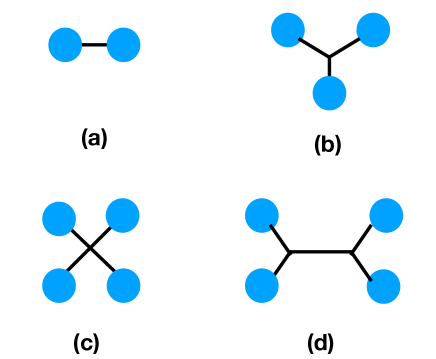
Figure 2: (Color online) Diagrams representing the many-body interactions of the four-nucleon cluster. Blue circles are nucleons, black lines are propagators of the $\phi$ fields

We will use some results of our previous paper on the subject DeMartini and Shuryak (2020) based on PIMC simulations at appropriate temperatures and densities of BES freezeouts. For four-nucleon clusters we calculated the 9-dimensional effective volume of the precluster, entering the 4th-order virial coefficient. We have shown that while precluster phenomenon only contribute to multiplicity at a sub-percent level, its positive contribution to $kurtosis$ of the proton multiplicity distribution becomes of order one for collision energies at and below $\sqrt{s}=7.7$ GeV, as it is indeed observed by STAR collaboration.

While in all these papers Shuryak and Torres-Rincon (2019, 2020a); DeMartini and Shuryak (2020) a variety of theoretical tools were used, the emphasis was on their consistency. Therefore the same $binary$ nuclear forces – the simplified Walecka model – were used in all of them. The issues of CP were addressed only peripherally, by binary forces modified by added exchanges of longer-range critical mode. Since the effect of that was persistently found to be catastrophic, it was clear that this approach could not possibly be an accurate description of the interactions near CP.

And indeed, as we will show in this paper, only with the inclusion of $many-body$ forces induced by critical fluctuations near the hypothetical CP resolves the puzzle. Furthermore, with presumed growth of the correlation length $\xi$, repulsive three and four-nucleon forces grow $stronger$ than binary ones, reversing the dependence on $\xi$. Basically, we will show that all preclustering should be suppressed in a small vicinity of CP. Thus, our calculations indeed predict strong $non-monotonous$ signal for BES, starting as an enhancement of clustering, to its full absence near the CP, and then back to enhancement at the other side of the CP.

(Before we begin our discussion, let us state for clarity that in this paper we are $not$ interested in the most generic problem of the many-body forces influencing the thermodynamics of infinite matter (at freezeout). Traditional studies of nuclear matter do include well documented three-body forces, derived from precise treatment of light nuclei. Those are not important here, since the nucleon density at freezeout conditions of heavy ion collisions of interest are even smaller than nuclear matter density. Also, as one can see below, the effects we discuss are much larger than those 3-body forces.)

Note that we discuss four-nucleon clusters with specific flavor-spin arrangement $p^{\uparrow}p^{\downarrow}n^{\uparrow}n^{\downarrow}$, with all four nucleons being distinguishable particles, so Pauli blocking is completely absent. This also simplifies combinatorial factors and reduced the technical challenges of the previous PIMC calculations.

The structure of the paper is as follows: in section II we introduce some lowest-order diagrams describing the interaction of the critical mode with nucleons and with itself, and qualitatively discuss their signs and magnitudes. Dependence of the diagram magnitude on the cluster size relative to the correlation length is discussed in section II.4. In the next section II.5 we average the diagrams over cluster shapes, using snapshots from the PIMC performed in Ref. DeMartini and Shuryak (2020). In section III we discuss the universal effective potential $\Omega(\phi)$ describing critical fluctuations on the critical line of Ising-class phase transitions. In section IV we consider a deformation of this potential by some external current $J$, shifting a bit from the critical line, and representing the freezeout path on the QCD phase diagram. Nonlinear coefficients of these deformed potentials are used as coupling constants in many-body diagrams. Combining those with the calculations of the diagrams themselves, we get to the results shown in Fig. 11. According to it, strong attraction due to exchange of the critical mode between the nucleons enhances clustering, with maximum at $t\approx 0.2$, and at smaller $t<0.11$ (closer to CP) it changes to repulsion, soon suppressing clustering. In section V we summarize the paper and discuss current status of relevant experimental observables.

II Three and four-nucleon forces and the four-nucleon clusters

II.1 Effect of critical binary potential

Refs. Shuryak and Torres-Rincon (2019, 2020a); DeMartini and Shuryak (2020) all discussed the effect of the the hypothetical critical point on nucleon interactions, but only via $binary$ forces. The critical fluctuations were assumed to add to conventional nuclear force a new binary potential corresponding to the diagram Fig. 2(a)

$$V_{a}=-g_{c}^{2}\langle\phi(\vec{r})\phi(0)\rangle=-{g_{c}^{2}\over 4\pi}{exp(-r/\xi)\over r}$$ (3)

Since this potential was included in the exponential of the action, all of its iterations were also included. The coupling of the critical mode to nucleons $g_{c}$ of course depends on the nature of the critical mode $\phi$. While in principle it can be estimated from mapping of Ising coordinates to QCD phase diagram, it does not belong to a class of observables uniquely predicted by universality arguments. One perhaps can view $\phi$ as having some admixture of the lowest (isoscalar) mesons $\sigma,\omega$, (or more precisely, the lowest-mass edge of the corresponding spectral densities). But, since the couplings to them have opposite sign, the magnitude of $g_{c}$ is hard to estimate, and we will use it as a free parameter.

As shown in all these works Shuryak and Torres-Rincon (2019, 2020a); DeMartini and Shuryak (2020), such approach leads to huge effects, which were judged to be unrealistic. Indeed, if the correlation length grows to $\xi>2\,fm\sim 1/(100\,MeV)$, all six pair terms in a four-nucleon cluster are comparable, leading to large correlation $\sim exp(6|V_{a}|/T)$.

In fact, it has been noticed previously by one of us Shuryak (2006) that such approach would lead to catastrophic phenomena when $\xi\rightarrow\infty$. Indeed, in this limit we will have attractive Newton-like potential between all nucleons in the fireball acting $coherently$. Since the total number of nucleons in the fireball is $N=O(100)$, the number of pairs $N(N-1)/2$ is so huge that for any meaningful $g_{c}$ (larger than QED electric coupling) one faces a (gravitation-style) collapse of the system! Looking for effects which can prevent this from happening, one naturally should consider the multi-nucleon forces.

II.2 Qualitative discussion of the multibody effects

Before we discuss phenomena associated with the critical point, let us recall how the usual nuclear potential and related clustering enter the thermodynamics. As explained in detail in our previous work DeMartini and Shuryak (2020), the 4-body clusters made of 4 distinguishable nucleons contribute the potential energy part of the statistical sum in the form of the fourth virial coefficient.

The potential part of the partition function (of a single species system) of $N$ particles can be re-written in the form

$$Z_{pot}=1+{1\over V^{N}}\int d^{3}x_{1}...\int d^{3}x_{N}\big{[}e^{\big{(}-\sum_{i>j}V(\vec{x}_{i}-\vec{x}_{j})/T\big{)}}-1\ \big{]}$$ (4)

by adding and subtracting 1. Since we focus on clusters of distinguishable 4 particles, coordinates of all others can be integrated out, as well as the coordinates of its center of mass. What is left is

$$Z_{pot}=1+\big{(}{N\over 4}\big{)}^{4}({V_{cor}\over V^{3}})$$ (5)

where the so-called 9-dimensional correlation volume is

$$V_{cor}^{(9)}=\frac{32}{105}\pi^{4}\int d\rho\rho^{8}(P(\rho)-1).$$ (6)

Here $P(\rho)$ is the probability distribution in the 9-dimensional hyperdistance $\rho$ normalized to that of a non-interacting ideal gas, and the factor in front is the solid angle in 9 dimensions. We neglect repulsion and integrate over the region in which the integrand is positive. The addition to the free energy is then $\Delta(-Tlog(Z))=-Tn^{3}V^{(9)}_{cor}{N\over 4^{4}}$, same as to the grand partition sum. Differentiating it with respect to $\mu$, present in each $N$, one finds the addition to particle number $\Delta N/N=n^{3}V^{(9)}_{cor}/4^{3}$ .

The magnitude of this effective volume depends on the temperature and density of the matter, and it was calculated in our PIMC simulations DeMartini and Shuryak (2020). For example, at kinetic freezeout conditions of $\sqrt{s}=7.7$ GeV, we found

$$V_{cor}^{(9)}(7.7)\approx 4.3\cdot 10^{4}\,fm^{9}$$ (7)

To put it in proper prospective, one can define the “density of the cluster” as

$$n_{cl}\equiv{4\over\big{(}V_{cor}^{(9)}\big{)}^{1/3}}$$ (8)

which for $\sqrt{s}=7.7$ GeV is $n_{cl}\approx 0.114\,/fm^{3}$. This value is about 3 times the density of ambient matter $n_{B}(7.7)\approx 0.037\,/fm^{3}$.

In our previous work, the PIMC action included only the binary forces between nucleons, either the standard ones (simplified to the Walecka form), or modified due to chiral crossover via reduced sigma mass. In this work our task is to include the many-body forces appearing near the hypothetical critical point.

Since below we will need to compare the inter-nucleon separations to the critical correlation length $\xi$, we will also define it by a cubic root of the respective densities

$$R_{amb}\equiv n_{B}^{-1/3}\approx 3.0\,fm,\,\,\,\,\,\,R_{cl}\equiv n_{cl}^{-1/3}\approx 2.0\,fm$$ (9)

The difference between these values may not appear to be large, but it would turn out to be crucial, as it will enter the relevant formulae in large powers. We do not yet know if the CP exists or not on the phase diagram, and we do not know what magnitude its maximal correlation length $\xi$ may reach on the freezeout line. For estimates we will assume that $\xi_{max}\sim 2\,fm$ can be reached, the value comparable to $R_{cl}$ defined above. As we will see, at such value the multibody forces are important for clusters but $not$ for ambient matter.

Let us now approach the critical point effects, using first the simplest approach available, known as Landau’s mean-field model. We also assume, for simplicity, that the freezeout and crossover transition line coincide. If so, the effective potential has $\phi\rightarrow-\phi$ symmetry and therefore odd powers of it must vanish, $\lambda_{3}=0$ and with it $V_{b},V_{d}=0$ ($V_{i}$ are the interactions of diagram (i)). Traditionally the Landau potential has only the mass term and nonzero 4-point vertex coupling $\lambda_{4}$. (Yes, we know the Landau potential does not correspond to CP, and nowadays is only used as the initial conditions for RG flow calculations. We will discuss proper critical potential below.)

This approximation leaves us with only two terms: the attractive two-body term $V_{a}\sim n_{B}^{2}$ and the repulsive four-body term $V_{c}\sim\lambda_{4}n_{B}^{4}$. At the small density of ambient matter, $n_{B}$ is small and the former dominates, while at the high density of the cluster, the latter dominates.

The free energy per particle is

$${F\over N}\sim-{g_{c}^{2}\over R}\big{(}{\xi\over R}\big{)}^{2}+{\lambda_{4}g_{c}^{4}\over R}\big{(}{\xi\over R}\big{)}^{8}.$$ (10)

In an Ising-type critical point in fact the quartic coupling vanishes, as $\lambda_{4}\sim 1/\xi$, making the effective power of it in the last term seven, not eight. Still, the dependence on $\xi$ is the same: negative at small $\xi$ is reversed to large and positive as $\xi$ grows. This means CP should suppress preclustering and thus reduce feed-down from the $4N$ system!

The magnitude of the couplings $g_{c}$, $\lambda_{4}$ are not yet known, but the effects of the $\xi/R$ ratios can be calculated. While in clusters this ratio is just about 1, with all its powers, for ambient matter these two terms have them be equal to

$$\big{(}{\xi_{max}\over R_{amb}}\big{)}^{2}\approx 0.444,\,\,\,\big{(}{\xi_{max}\over R_{amb}}\big{)}^{7}\approx 0.058$$ (11)

and the many-body repulsion term is relatively small.

The critical fluctuation effects thus can work $against$ clustering, reducing the cluster volume $V_{cor}^{(9)}$, and thus leading to a $reduction$ of the kurtosis. Note, that this approximation corresponds to approaching the CP from smaller to large density, or $\mu_{B}$, or approaching with collisions at energies $above$ that of CP.

II.3 Multibody forces in four-nucleon clusters

In general, the potential part of the partition function should include both binary and many-body forces. While the former ones were included in PIMC simulations, the latter were not there. Our task in this work to do so, in particular for the many-body forces appearing due to nonlinear effective Lagrangian of the critical mode.

Let us introduce the notations we use. For three-body forces induced by diagram (b) we define function

$$V_{b}\big{(}\vec{x}_{1},\vec{x}_{2},\vec{x}_{3}\big{)}\equiv\int d^{3}uD(\vec{x}_{1}-\vec{u})D(\vec{x}_{2}-\vec{u})D(\vec{x}_{3}-\vec{u})$$ (12)

where

$$D(r)=exp(-r/\xi)/r$$ (13)

is the binary Yukawa potential. Note that this function is dimensionless, and that we do not include here the factor $1/4\pi$ present in 3d propagator, which will be included later with the couplings.

Similarly, we define four-body function for diagram (c), we have

$$V_{c}\big{(}\vec{x}_{1},\vec{x}_{2},\vec{x}_{3},\vec{x}_{4}\big{)}\equiv\int d^{3}uD(\vec{x}_{1}-\vec{u})D(\vec{x}_{2}-\vec{u})D(\vec{x}_{3}-\vec{u})D(\vec{x}_{3}-\vec{u}).$$ (14)

Note that its dimension will be $[fm^{-1}]$.

Finally, for diagram (d) we define

$$V_{d}\big{(}\vec{x}_{1},\vec{x}_{2},\vec{x}_{3},\vec{x}_{4}\big{)}\equiv\int d^{3}ud^{3}vD(\vec{x}_{1}-\vec{u})D(\vec{x}_{2}-\vec{u})D(\vec{u}-\vec{v})D(\vec{x}_{3}-\vec{v})D(\vec{x}_{4}-\vec{v})$$ (15)

with corresponding dimension $[fm]$.

These functions depend on the coordinates of 3 or 4 nucleons, and should be averaged over many-body density matrix $P\big{(}\vec{x}_{1},\vec{x}_{2},\vec{x}_{3},\vec{x}_{4}\big{)}$ of the clusters.

Using these definitions, we can write the effective potential for four-nucleon cluster in the following form

$$V_{abcd}= -{4\cdot 3\over 2}{g_{c}^{2}\over 4\pi}{exp{(-r_{ij}/\xi)}\over r_{ij}}+4\cdot 3!\lambda_{3}({g_{c}\over 4\pi})^{3}V_{b}$$ (16)

$$+4!\lambda_{4}({g_{c}\over 4\pi})^{4}V_{c}-4!{\lambda_{3}^{2}\over 8\pi}({g_{c}\over 4\pi})^{4}V_{d},$$

where we have now restored combinatorial factors and signs. All interactions $V_{i}$ generically depend on all nine hypercoordinates, although we will make simplifying assumptions later. Note that an extra $1/8\pi$ in the last term comes from $1/2!$ of the second order expansion and $1/4\pi$ from an extra intermediate propagator between the vertices.

Generally speaking, this many-body potential should be included in PIMC simulations, as it was done with the binary potential, to directly observe its effect on clustering. It is not however practical to do so as they include extra multidimensional integrations over the locations of the nonlinear vertices, and are thus too computationally intensive at present.

We therefore adopt the perturbative approach, in which all locations of the nucleons $\vec{x}_{i}$ in the cluster are to be averaged over the appropriate 9-dimensional density matrix calculated in PIMC with the binary interactions only .

In doing this average, we would like to separate the dependencies on the “hyperdistance” $\rho$ and the “shapes” (angular variables) of the cluster. The former is defined via most-symmetric definition of the hyperdistance $\rho$ (41) coordinate.

II.4 Dependence of multibody forces on the cluster shape and the correlation length

As a warm-up, we calculate the diagrams for two specific shapes. The most symmetric one is a $tetrahedral$ shape, in which all pair distances are the same $L_{tet}$. Another shape we considered is a flat square with size $L_{sq}$: in order for both to correspond to the same hyperdistance $\rho$, they should be related by

$$6L_{tet}^{2}=(4+2\cdot 2)L_{sq}^{2}=4\rho^{2}$$ (17)

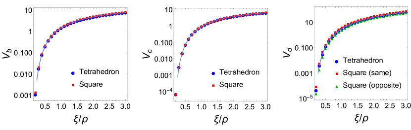
Figure 3: (Color online) Interactions $V_{b}$ (left), $V_{c}$ [fm^-1] (center), and $V_{d}$ [fm] (right) corresponding to diagrams (b,c,d) of Fig. 2, respectively, as a function of the correlation-length-to-hyperdistance ratio $\xi/\rho$ for both the tetrahedral and square configurations. The curve is an interpolation of the tetrahedral data points. The distinction between the ’same’ and ’opposite’ square configurations for diagram (d) is explained in the text.

The results are shown in Fig. 3 as a function of the basic ratio $\xi/\rho$, and also in Table 1 for $\xi/\rho=1$ . In diagram (d) there are two vertices and the square configuration can be further divided into two more configurations: one in which nucleons on the same side of the square are connected to the same vertex and one in which nucleons on opposite corners are connected. The same distinction can be made for the binary interaction (diagram (a)), where two nucleons on the same or opposite side of the square can be connected by the propagator. While $V_{b}$ and $V_{c}$ show very small dependence on cluster shape, it is not so for $V_{d}$. Both the tetrahedron and square are very symmetric configurations and we know from the previous work that even in the correlated cluster, there are not significant angular correlations between the nucleons.

Using these results and assuming, for simplicity, a Landau form of effective action, with only diagrams (a) and (c) included, one can access the dependence of the cluster potential on the magnitude of the correlation length $\xi$. Assuming further that all clusters have the same tetrahedral shapes, we define the average potential as

$$V_{tet}=-6{g_{c}^{2}\over 4\pi}\langle V_{a}\rangle+4!\lambda_{4}({g_{c}\over 4\pi})^{4}\langle V_{c}\rangle$$ (18)

Now we need to select reasonable values for the couplings. Some guidance on the magnitude of $g$, the coupling of $\phi$ to the nucleon, can be obtained from the Walecka model applications to nuclear matter. In it the sigma and omega couplings are

$${g_{\sigma}^{2}\over 4\pi}=6.04,\,\,\,\,{g_{\omega}^{2}\over 4\pi}=15.17.$$ (19)

The critical mode $\phi$ is presumably some superposition of the (lowest-momenta parts of the spectral densities) with $\sigma,\omega$ quantum numbers. So, its coupling must be comparable. As a guess, in literature some round intermediate number

$${g_{c}^{2}\over 4\pi}=10$$ (20)

was used, and we take this value in estimates to follow.

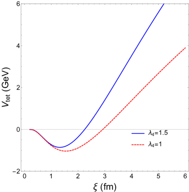
Figure 4: (Color online) Energy of four-nucleon tetrahedral cluster $V_{tet}$ of size $\rho=2$ fm as a function of correlation length $\xi$. The critical mode-nucleon coupling is taken to be equal to nucleon-sigma meson coupling of the Walecka model (19), and two values of the four-point coupling $\lambda_{4}$ are used.

The value of quartic coupling $\lambda_{4}$ in the Landau model remains an arbitrary parameter. So in Fig. 4 we show the dependence of the additional cluster energy (18) as a function of the correlation length, for its two values. Naturally, at small $\xi$ all forces are very short range and additional energy is very small. With $\xi$ growing to about 1.5 fm the six attractive potentials reach together a value of the order of $-1$ GeV, but for larger $\xi$ values the quartic term mitigates attraction and turns the curve upward, eventually making this additional energy positive. A similar trend would be seen for any other cluster shape. This provides some initial understanding of possible role of the many-body forces.

II.5 Averaging the multi-body forces over PIMC clusters

To make the analysis of the previous section a bit more quantitative, one needs to understand the effect of averaging over all cluster shapes. In order to do so we use the 9-dimensional configurations taken from PIMC simulation at a fixed value of $\rho$ and calculates all 4 diagrams for them. The distribution of values is shown in Fig. 5. One finds that in fact there where a wider distribution of values is seen than for the fixed shapes discussed before. For all three diagrams, variation by $\sim 50\%$ is seen from changing the shape but keeping $\rho$ fixed. This indicates that an accurate parameterization of these interactions requires not just dependence on hyperdistance $\rho$, but rather they must depend on the full set of $9$-dimensional hypercoordinates. However, we find that there is overall less sensitivity to system shape than to other quantities in the energy of the cluster, such as the nucleon-critical mode coupling $g_{c}$ or the external current $J$ (see Section IV). Because the dependence on cluster shape is rather weak, we assume that the average interactions over all shapes is equal to that of the tetrahedral cluster of the same size, $\langle V_{i}(\xi/\rho)\rangle=V_{i,tet}(\xi/\rho)$.

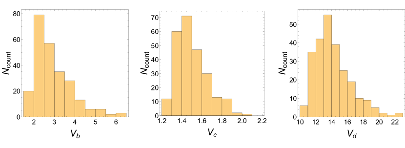
Figure 5: Distribution of values of the multibody interactions $V_{b}$ (left), $V_{c}$ (center), and $V_{d}$ (right) corresponding to diagrams (b,c,d) of Fig. 2, respectively, in 250 configurations generated in PIMC simulation. All configuration have $1.49<\rho<1.51$ (fm) and were computed with $\xi=2$ fm.

After these preliminary studies of the diagrams for clusters of particular shapes, we perform the actual density matrix from our PIMC ensemble DeMartini and Shuryak (2020). The results are shown as histograms of the values of the potentials $V_{i}$, for configurations. The cluster configurations are chosen from those with $\rho<3$ fm, the approximate maximum size of the cluster. Ambient configurations are then chosen from those with $\rho>3$ fm, where the average inter-nucleon binary interaction is small $\langle V_{NN}\rangle\simeq 0$ and no correlation is observed. For each set 5000 configurations are chosen from the PIMC simulation corresponding to conditions of kinetic freezeout at $\sqrt{s}=7.7$ GeV. As expected, these values are quite different for these two subsets, indicating that many-body forces are much more important within the clusters than for random (uncorrelated) nucleons.

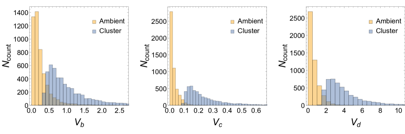
Figure 6: (Color online) Distribution of values of the multibody interactions $V_{b}$ (left), $V_{c}$ (center), and $V_{d}$ (right) corresponding to diagrams (b,c,d) of Fig. 2, respectively, in 5000 configurations each for the cluster ($\rho<3$ fm) and ambient nucleon matter ($\rho>3$ fm) generated in PIMC simulation. Calculation performed with $\xi=2$ fm.

The results are plotted at Fig. 6. These histograms show that the many-body interactions are much stronger in the cluster compared to the ambient matter at freezeout. The distributions in the cluster possess both larger average values of the interactions and much longer high-value tails than the ambient matter distributions. The long tails of these distributions correspond to the most compact clusters (with the smallest values of $\rho$).

Comparing the average values of the interactions, one finds

$$\frac{\langle V_{a}\rangle_{cl}}{\langle V_{a}\rangle_{amb}}=2.63,\,\,\,\frac{\langle V_{b}\rangle_{cl}}{\langle V_{b}\rangle_{amb}}=4.00,\,\,\,\frac{\langle V_{c}\rangle_{cl}}{\langle V_{c}\rangle_{amb}}=10.73,\,\,\,\frac{\langle V_{d}\rangle_{cl}}{\langle V_{d}\rangle_{amb}}=6.52.$$ (21)

As expected, there is a clear hierarchy in these ratios. The dependence of the $N$-body diagrams on the ratio $\xi/\rho$ grows with $N$. Thus, the many-body interactions grow in their importance relative to the standard binary interaction as $\xi$ increases near CP. These ratios should grow at smaller values of row such as $\rho\sim 1.5$ fm, where peak spatial correlation is observed.

Table 1: The first two rows are the average values of the diagrams in both the cluster and ambient nucleon matter computed with $\xi=2$ fm. Latter three rows are the values of the diagrams for the specific geometries calculated with $\xi/\rho=1$. All values are given without couplings, combinatorial factors, signs, and factors of $4\pi$ in propagators: e.g. $V_{a}$ are given without $-g_{c}^{2}/4\pi$.

	a	b	c	d
$\langle V\rangle_{cl}$	0.110	1.092	0.292	4.184
$\langle V\rangle_{amb}$	0.289	0.273	0.027	0.642
$V_{tet}$	0.541	1.434	0.924	3.143
$V_{sq,same}$	0.697	1.485	0.956	3.713
$V_{sq,opp}$	0.368	-	-	2.523

III The universal effective action for Ising-type critical fluctuations

The Landau model, used as an initial approximation, does $not$ however represent correct behavior near Ising-like critical points. Wilson’s expansion in $\epsilon=4-d$ ($d$ is space dimension) has found that under the renormalization group flow the Landau model goes into the fixed-point regime in infrared, with small coupling $\sim\epsilon$. While Wilson famously calculated approximate values of the critical indices for $d=3$, further series in $\epsilon$ do not show good convergence and led to doubts about its accuracy at $\epsilon=1,d=3$.

Exact renormalization group equations were derived, using Wetterich exact RG equations, and its solution for $d=3$ were worked out, for recent reviews see Refs. Berges et al. (2002); Dupuis et al. (2020). Unfortunately, obtaining the near-fixed-point solution can not be done analytically, and therefore one relies on certain fits.

We will also use certain simplifying approximations. We will ignore renormalization of the propagator and its index $\eta$, putting it to zero. So, the kinetic term will be kept in its initial form $(\partial\phi)^{2}/2$, and the propagators will be kept in their Yukawa form.

The effective vertices (powers of $\phi$ larger than 2) we get from local form of the effective action $\Omega(\phi)$, will be obtained from fluctuation potential for homogeneous constant fields $\phi(x)\rightarrow\langle\phi\rangle$. The partition function in the $x$-independent form is just

$$Z(J)=\int D\phi e^{(-\Omega(\phi)+J\phi)V_{3}/T},$$ (22)

where $V_{3}$ is the volume of the system and $T$ is temperature, and the functional form of $\Omega(\phi)$ can be deduced from dependence on the external current $J$.

We start with brief qualitative discussion of possible form of this effective potential $\Omega(\phi)$ near CP, mentioning few “folklore” arguments suggesting that $\Omega$ is effectively given by a polynomial of order 6. If one “probes” $\Omega(\phi)$ by a nonzero external term $J$, the mean “magnetization” $\langle\phi\rangle(J)$ index $\delta$ is defined as

$$\langle\phi\rangle(J)\sim J^{1/\delta},\,\,\,\delta={d+2-\eta\over d-2+\eta}\approx 4.78.$$ (23)

The number on the r.h.s. is empirical, from real and numerical experiments for various systems belonging to Ising universality class.

The minimum of the potential shifted by $J\neq 0$ is given by the solution of

$${d\Omega\over d\phi}=J.$$ (24)

For $m\rightarrow 0$ and Landau theory, when the only nonlinear term is $\phi^{4}$, one finds $\delta=3$, which is not close to the true value. The closest integer to 4.78 is 5. (Note that it corresponds to neglecting the $\eta\rightarrow 0$ in general expression above, which we assumed anyway for propagators.) If so, it implies that $\Omega\sim\phi^{6}$. One can therefore think that a potential being a polynomial of order six would be a good approximation to reality.

The second argument is theoretical: including a $\phi^{6}$ term – but not higher powers – can be justified because this term is the last renormalizable one, in $d=3$ space.

There are of course multiple numerical studies of the Ising model suggesting various fits of $\Omega(\phi)$, at many lattices and $J$ values. In particular, good quality fits were reached in Ref. Tsypin (1994), after the pre-exponent factor $\sqrt{d^{2}V/d\phi^{2}}$ was included. We will follow this paper, in which

$$\Omega(\phi)=\int d^{3}x\big{[}{(\partial_{\mu}\phi)^{2}\over 2}+{m^{2}\phi^{2}\over 2}+mg_{4}\phi^{4}+g_{6}\phi^{6}\big{]}.$$ (25)

Note that quartic term in it is proportional to the $first$ power of the same $m$ as is quadratic in the $\phi^{2}$ term. Indeed, at CP, when $m\rightarrow 0,\xi\rightarrow\infty$, only the $\phi^{6}$ term remains.

(A side comment: numerical simulations of Ref.Tsypin (1994) are done for several lattices, but with constant ratio of the box size $L$ to the correlation length $\xi$, specifically $L/\xi=4.1$. This implies existence of about $(L/\xi)^{3}\sim 70$ statistically uncorrelated domains. Curiously, by numerical coincidence, a similar ratio (and number of domains) are expected for fireballs corresponding to central heavy ion collisions and $\xi_{max}\sim 2\,fm$. Therefore, histograms for mean field distributions $P(\phi)\sim exp[-V_{4}\Omega(\phi)]$ from the paper are approximately the same as in these fireballs.)

Unlike in familiar 4 dimensions, in the $d=3$ setting of the Ising class we discuss the dimension of the field is $[\phi]\sim L^{-1/2}$. Therefore all terms in (25) scale as $L^{-3}$ for dimensionless couplings $g_{4},g_{6}$. In order to make field also dimensionless, let us define a scale $M$ by the beginning of near-$T_{c}$ scaling relation with critical index $\nu$ of the correlation length

$$m={1\over\xi}=Mt^{\nu}$$ (26)

where we use standard dimensionless temperature variable $t\equiv(T/T_{c}-1)$. Let us also use it to define dimensionless field

$$\tilde{\phi}\equiv{\phi\over M^{1/2}}$$ (27)

and rewrite potential for constant field as

$$\Omega(\phi)=(V_{3}M^{3})\big{[}{t^{2\nu}\tilde{\phi}^{2}\over 2}+g_{4}t^{\nu}\tilde{\phi}^{4}+g_{6}\tilde{\phi}^{6}\big{]}$$ (28)

The coupling values obtained by Tsypin are

$$g_{4}=0.97,\,\,\,g_{6}=2.05$$ (29)

We also compared these lattice fits with exact RG solutions summarized in Ref. Berges et al. (2002). From discussion in section 4.4 of that paper we extracted their polynomial fit, to

$${\partial U\over\partial\phi}\sim(a_{0}s+a_{1}s^{3}+a_{2}s^{5}+a_{3}s^{7})$$ (30)

where $s$ is their re-scaled $\phi$. The fitted values are

$$a_{0}=1.0084;\,a_{1}=3.1927;\,a_{2}=9.7076;\,a_{3}=0.5196$$

A drop from the six-field coefficient $a_{2}$ to the eight-field coefficient $a_{3}$ by a factor 20 confirms that truncation of the eight-field term is indeed justified, as are that for higher orders not used in the fit. Furthermore, the values of other coefficients are in a reasonably good agreement with (29).

The scale $M$, defining the absolute size of the scaling window. Below for estimates we will use $M=m_{\sigma}\approx 500$ MeV, which implies that at the edge of this window, $\xi(t=1)=0.4\,fm$, the $\phi$ exchange range is the same as in Walecka sigma meson exchange (which we subtract from the contribution of diagram (a) in forthcoming calculations of $\Delta F$). So, with this choice we have zero effect at $t=1$ from (a) and negligible many-body forces. It is of course not universal, and it can be that scaling window is smaller, e.g. $M\sim 1fm^{-1}$.

For orientation, with such choice of scale, the value $\xi=2\,fm$ (comparable to the cluster sizes) corresponds to $t^{\nu}\approx 1/5$ or $t\approx 0.077$. The calculations and plots below, e.g. Fig. 11, are done for $t$ ranging from 0.077 to 0.5.

The probability distribution depends on a prefactor of the scaled effective potential, the 3D volume $V_{3}$ over which fluctuations are measured and $T$, in units of $M^{3}$ and $M$ respectively. For estimates one may take $V_{3}$ to be the volume of ”preclusters” and use the kinetic freezeout temperature $T\approx 120$ MeV. The resulting distribution is plotted in Fig. 7.

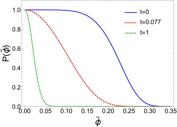
Figure 7: (Color online) The universal probability distributions of dimensionless $\tilde{\phi}$ field. Far from CP corresponds to $t=1$ with Gaussian-like distribution, maximum expected correlation length $\xi=2$ fm corresponds to $t=0.077$, and CP corresponds to $t=0$, here critical fluctuations are maximal and strongly non-Gaussian.

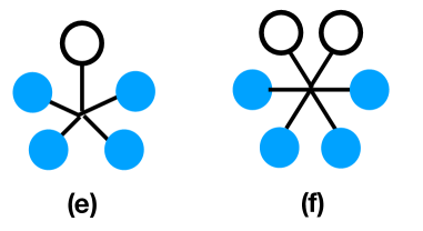
Figure 8: Lowest order diagrams including five and six nucleons. Closed circles are those belonging to 4-N cluster, open circles indicate nucleons from the “ambient matter”

The assumed dominance of the 6-field coupling puts into question whether the original 4 diagrams of Fig. 2 would be enough, especially very close to the CP. Therefore we introduce two more, shown in Fig. 8. The diagram (f) for uncorrelated nucleons (4 in the cluster and 2 in ambient matter) can be estimated as

$$V_{f}/n\sim{g_{c}^{6}\over R_{cl}}g_{6}\big{(}{\xi^{12}\over R_{cl}^{9}R_{amb}^{3}}\big{)}$$ (31)

with two last brackets dimensionless. So, for $\xi\ll R_{cl}<R_{amb}$ it is extremely strongly suppressed, but if $\xi\sim R_{cl}\sim 2\,fm$ most of the suppression is gone. It is this repulsive diagram alone which should be able to moderate huge attraction due to diagram (a) at the CP.

IV Deformed effective potential near the critical line

The universal effective potential discussed in the preceding section (25) was defined $on$ the critical line. Therefore it was symmetric under $\phi\rightarrow-\phi$ and included only $even$ powers of $\phi$. However, in heavy ion collisions we expect the endpoints of evolution paths on the phase diagram, known as the freezeout line, to be located at certain distance $below$ ( at lower $T$) critical line. Such shift modifies the effective potential. In particular, the maximal value of the correlation length $\xi=1/m$ gets limited. Also the $\phi\rightarrow-\phi$ symmetry is broken and odd powers of $\phi$ appear. As we now detail, it turned out to be very important for the estimated many-body forces.

We thought of two approaches to define the $deformed$ effective potential:
(1) One general way is to start with the universal Equation of State (EOS) on the 2D plane of the Ising variables, the reduced $t$ and the magnetization $M$, and then map it to QCD phase diagram. This approach, started in the epsilon-expansion framework, was used by Nonaka and Asakawa Nonaka and Asakawa (2005), and Stephanov Stephanov (2011). We followed it to some extent, and put some the related formulae and one plot in Appendix C.
(2) Another is to use the effective potential on the critical line, defined in the previous section, and calculate its deformation by a linear term $J\phi$, assuming that $J$ remains constant at the freezeout line. Using it, we calculate the deformation of effective potential shape and then use the coefficients of $\phi^{3},\phi^{4}$ as effective nonlinear couplings $\lambda_{3},\lambda_{4}$.

The first effect of the deformation by $\tilde{J}\tilde{\phi}$ term is a shift of the maximum away from the symmetry point $\phi=0$. Location of the new maximum $\tilde{\phi}_{0}(\tilde{J})$ is to be found from solving polynomial equation

$${\partial\Omega_{def}\over\partial\tilde{\phi}}(\tilde{\phi}_{0})=\tilde{J}$$ (32)

which, with our truncation, is of the 5th order. As an example, for $\tilde{J}=1/100$ we perform this procedure for various values of $t$. In particular, the real roots of this equation are

$$\tilde{\phi}_{0}(t=0.01)\approx 0.224,\,\,\,\tilde{\phi}_{0}(t=0.41)\approx 0.031$$

We then rewrite the fluctuation field in the form

$$\tilde{\phi}=\tilde{\phi}_{0}+\delta$$ (33)

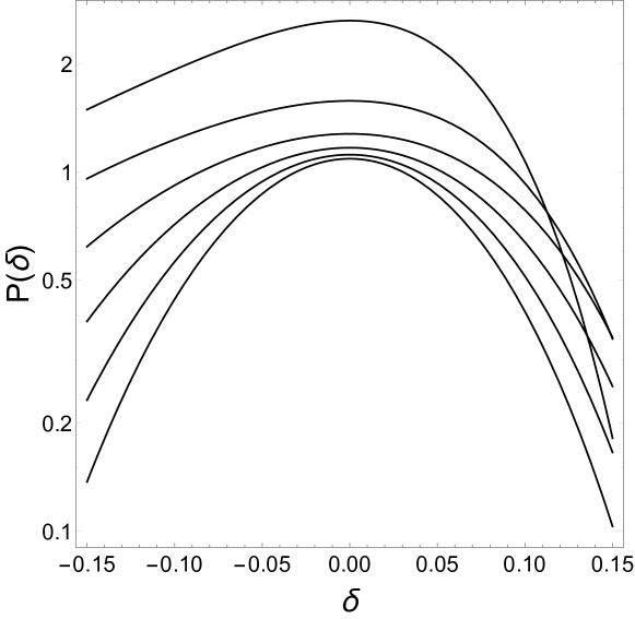
Figure 9: Probability distributions of the deformed action $P(\delta)$ distorted by $\tilde{J}=0.01$ in the 4-nucleon cluster volume. The six curves, from top to bottom, correspond to values of $t=0.01,0.09,0.17,0.25,0.33,0.41$, respectively. The 3D volume and mass prefactors are explained in the text.

and re-express the potential in terms of new fluctuation field $\delta$. This was done for all values of $t$, for example the deformed potential at $t=0.01$ takes the form

$$\Omega_{def}(t=0.01)\approx-0.0017+0.095\delta^{2}+0.51\delta^{3}+1.60\delta^{4}+2.75\delta^{5}+2.05\delta^{6}$$

Note that there is no linear terms, but other odd powers of $\delta$ are present.

In order to get an idea about actual distributions of the fluctuating critical field one has to return to dimensionful prefactor of the universal action, and also select the scale at which the fluctuations will be studied. The probability distribution of homogeneous fields is given in Eq. (34) where $V_{3}$ is the 3D volume, made dimensionless by the 3rd power of basic scale $M$. Using the volume of the cluster $V_{3}=(4.3*10^{4}$ fm${}^{9})^{1/3}$, one finds a very large product of the first bracket, $\sim 550$. Yet since small $\delta$ appears in high powers, one gets the distributions shown in Fig. 9. While it is approximately Gaussian for larger $t$ (bottom curves), it becomes quite strongly deformed close to CP.

The dependence of $m^{2}=1/\xi^{2}$, and the triple and quartic couplings from the deformed effective action on $t$ is shown in Fig. 10. Note significant growth of the coupling near CP (left). Note also that at small $t$ the inverse correlation length $m$ does not go to zero, although it remains small.

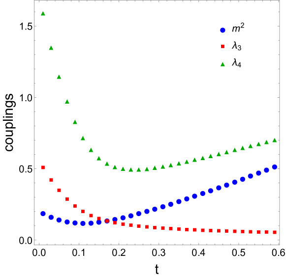
Figure 10: (Color online) The dependence of $m^{2}=1/\xi^{2}$, and the triple and quartic couplings, for the effective action deformed by $J=1/100$, on scaled temperature $t$.

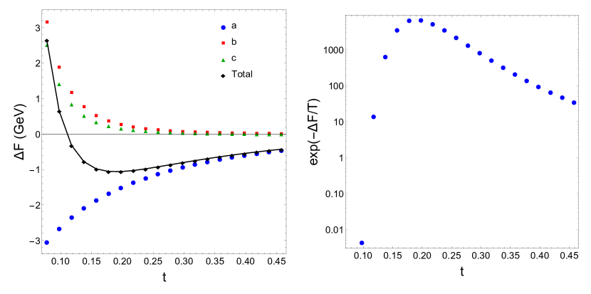
Figure 11: (Color online) Left plot: contributions to the change in free energy $\Delta F$ of a 4-nucleon cluster of size $\rho=2$ fm due to individual diagrams (a,b,c) and their total combined contribution, with coupling $g_{c}^{2}/4\pi=10$, versus $t=T/T_{c}-1$. Diagram (a) has had the unmodified binary interaction subtracted out as described in the text. Right plot: Boltzmann factor of the change in potential $\exp(-\Delta F/T)$ with $T=120$ MeV, versus t. Note that the leftmost point, $t=0.077$ (not shown) has Boltzmann factor $\simeq 10^{-10}$.

$$P(\delta)\sim exp\big{[}-(V_{3}M^{3})\Omega_{def}(\delta)\big{]}$$ (34)

Unfortunately, the real fluctuating fields are not homogeneous, and so these distributions serve only for orientation. What one needs to do is to evaluate the diagrams with propagators containing appropriate correlation length for each $t$. The value of the nonlinear couplings $\lambda_{3},\lambda_{4}$ should be taken as coefficients of $\delta^{3},\delta^{4}$ terms. In the case of $\lambda_{3}$ a factor of $M$ is inserted to restore it to its dimensionful form.

The free energy density of a cluster divided by the nucleon density we define for binary term as follows

$$F_{a}=-{4\cdot 3\over 2}{g_{c}^{2}\over 4\pi r}exp\big{[}-rMt^{\nu}\big{]},$$ (35)

for three-body force as

$$F_{b}=4\cdot 3!\lambda_{3}M\big{(}{g_{c}\over 4\pi}\big{)}^{3}V_{b}(\rho Mt^{\nu}),$$ (36)

and for (diagram c) four-body force as

$$F_{c}=4!\lambda_{4}\big{(}{g_{c}\over 4\pi}\big{)}^{4}V_{c}(\rho Mt^{\nu}).$$ (37)

Here, inter-nucleon distance $r$ and hyperdistance $\rho$ are related as they are in the tetrahedral cluster, $r=\sqrt{2/3}\rho$.

Our task is now to combine all terms and see how they affect the 4-body clusters. In Fig. 11 (left) we show the results of our calculation of the free energies at ten values of $t$, increasing from $t_{min}=0.077$ and corresponding to diagrams (a,b,c), separately and in sum. A very large attractive contribution (calculated in some earlier works) is in fact compensated by 3- and 4-body repulsive terms, so that the sum becomes positive for $t<0.11$, before the maximal correlation length is reached.

The contribution of diagram (d)

$$F_{d}=-{4!\over 8\pi}\lambda_{3}^{2}M^{2}\big{(}{g_{c}\over 4\pi}\big{)}^{4}V_{d}(\rho Mt^{\nu})$$ (38)

is not included in the plot because it turned out to be small, well inside the uncertainties. In particular, its largest value (at $t_{min}$, the leftmost point in Fig. 11 (left)) is only $-164$ MeV.

Since, in the left plot of Fig. 11, it is hard to read the magnitude of the attractive effect on the r.h.s. , we separately show how this free energy translates into the probability of precluster production, $\exp(-\Delta F/T)$ in the right plot. In it one finds that attractive force is strong enough to enhance clustering, by a few orders of magnitude at distance $t=0.2$ from the CP. At the same time it plunges well below 1 due to repulsive many-body forces at smaller $t$ (closer to the CP). This is the “non-monotonous signal” we speak about.

Let us remind that very strong effects displayed in Fig. 11 were shown as a function of $t$, on a line close to the critical line distorted by $\tilde{J}=1/100$, for clusters of fixed size $\rho=2\,fm$. We selected this size as characteristic of pre-clusters as PIMC calculation with conventional nuclear forces.

Another perspective on the problem is obtained if one fixes $t$, say to values rather close to CP, just above $t=0.077$ with correlation lengths just below $\xi=2$ fm, and plot the total energy of the cluster as a function of its size $\rho$, see Fig. 12. One can see from it that while for $\rho<2$ fm the potential is indeed repulsive and much larger than $T\sim 100$ MeV, it is very rapidly changing for larger sizes. As one approaches CP, the size of this repulsive region increases and the maximum depth of the attraction decreases. In particular, near the minimum at $\rho\approx 4$ fm, $-\Delta F/T\approx 2$ at the smallest value of $t$. Therefore, here instead of suppression one finds enhancement in the production of clusters of a larger size relative to PIMC is by factor $\exp(2)\sim 7$, rather than by three orders of magnitude, as in Fig. 11. This qualitative behavior remains unchanged for different reasonable choices of the nucleon-critical mode coupling. Varying this coupling modifies the size of the repulsive region, while keeping the maximum depth of the attraction relatively fixed, as seen in Fig. 12 (right).

It might be tempting to conclude that accounting for many-body forces simply modifies clusters to be of the size $\rho>3$ fm rather than $\sim 2$ fm as was seen in PIMC calculations. Such a conclusion would however be rather meaningless, since at such size the effective cluster density would not be any different from that of ambient matter. In other words, there would be enhancement, but feed-down from such large clusters to light nuclei production would be negligible, as the clusters are much larger than the excited ${}^{4}He$ states which feed down into light nuclei.

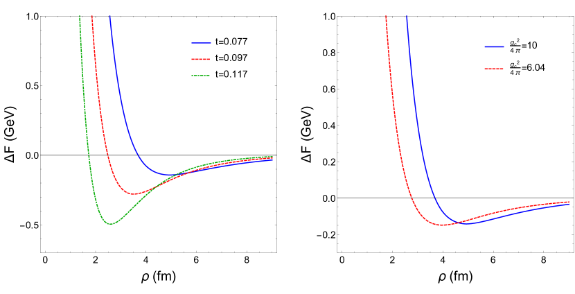
Figure 12: (Color online) Left plot: The change in effective potential $\Delta F$ as a function of cluster size $\rho$ with $g_{c}^{2}/4\pi=10$ for three values of scaled temperature $t$. Right plot: The change in effective potential $\Delta F$ as a function of cluster size $\rho$ at $t=0.077$ for two values of the nucleon-critical mode coupling $g_{c}$. In both plots, diagram (a) has had the unmodified binary interaction subtracted out as described in the text.

Concluding our calculations, we remind the reader that while in this paper we focused only on 4-body clusters, there are of course larger ones. For them one should also include five and six-body forces. Note that the deformed effective action predicts them to be also repulsive, and even larger . Therefore, our main finding – suppression of all forms of clustering in the vicinity of the CP – should hold, even if all possible clusters are included.

V Summary, discussion and experimental observables

Let us start by reminding the reader the paradox (pointed out in Ref. Shuryak (2006)): the effect of binary forces induced by long-range critical mode at CP, with $\xi\rightarrow\infty$, is catastrophic. Indeed, if all $N(N-1)/2\sim 10^{4}$ pairs of nucleons in the fireball be attracted to each other by Newton-like potential, the fireball would implode, like in a gravitational collapse.

The resolution of this paradox is one of the main conclusions of this paper. Large correlation length $\xi$ generates also repulsive many-body forces, strong enough to mitigate the binary attraction and reverse the trend, $suppressing$ preclustering close to CP.

With this qualitative conclusion, let us discuss the uncertainties involved. Many features of the CP are known, as it is supposed to belong to the 3D Ising universality class. Yet some basic mass scale $M$ and the critical mode coupling $g_{c}$ are non-universal and remain unknown. Changing $g_{c}$ will modify the overall scale of the predicted effects, as $N$-body interactions depend on $g_{c}^{N}$. The mass scale $M$ appears directly in the 3-body term and affects the mapping between $t$ and $\xi$. While their values are not known, we have used physically-motivated estimates – the values should be comparable to the nucleon-sigma coupling $g_{\sigma}$ and the sigma mass $m_{\sigma}$, respectively. Additionally, the external current $\tilde{J}$ deforms the potential. At present, we have chosen $\tilde{J}$ to be small to reflect the closeness of the critical and freezeout lines. Fortunately, dependence on the specific value of $J$ is weak, e.g. $\langle\phi\rangle\sim J^{1/5}$. Needless to say, all such non-universal parameters may be fitted to the data, once the CP is found.

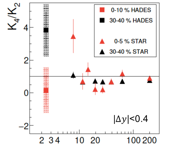
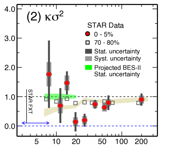
Figure 13: (Color online) Upper plot: The kurtosis ratio $K_{4}/K_{2}$ from STAR and Hades experiments, versus $\sqrt{s}$, from Adamczewski-Musch et al. (2020). Red points show the most central bins, black points for mid-central one, $30-40\%$.
Lower plot: more recent STAR results, corrected in Adam et al. (2020).

Let us now proceed to the status of experimental observables. The summary of kurtosis data of the net proton distribution is shown in Fig. 13. The upper plot is earlier summary, the lower one is from recent STAR publication Adam et al. (2020). More strict event selection applied have basically modified one point, the central bin of $7.7\,GeV$ run.

Interpreting summary plots one should keep in mind that detectors involved in these and next plots – STAR at BNL RHIC, HADES at GSI , NA49 at CERN SPS and ALICE at LHC – have completely different kinematic settings, acceptances and use different extrapolation procedures. Therefore, comparison of their points needs to be done with care. As one can see, the errors are still large. The lower plot indicate projected accuracy of BES-II program (green shaded area near 1).

On the other hand, inside each group the centrality bins are supposed to be processed in exactly the same way. If one trusts the centrality dependence of each set, one finds a striking $reversal$, between the STAR centrality dependence at $7.7\,GeV$ and that reported by HADES at $2.4\,GeV$. Also both plots show clear depletion near $20\,GeV$, in central relative to peripheral bins.

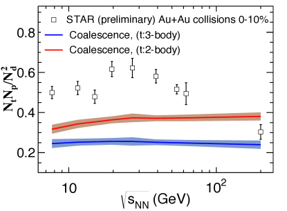
Figure 14: (Color online) Left plot: The ratio of yields of tritium, protons normalized to deuterium $t\cdot p/d^{2}$, from a cascade code Zhao et al. (2020), points are from STAR collaboration. Right plot: Compilation of experimental data for the same ratio from Shuryak and Torres-Rincon (2020b). Note that it has different range from the left plot, and is a log-log plot.

Another observable sensitive to preclustering is additional feed-down into production of light nuclei. The most sensitive to four-nucleon clusters are $t$ and ${}^{3}He$. The compilation of the data for the ratio of yields $N_{t}N_{p}/N_{d}^{2}$ from Shuryak and Torres-Rincon (2020b) is shown in Fig. 14.

This ratio is selected because in it the main driver of light nuclei yields – the factors of fugacity $exp(\mu/T)$ – cancel out. The left plot, from Zhao et al. (2020), is theoretical predictions resulting from a state-of-the-art cascade code. It reproduces many features of heavy ion collisions but does not have preclusters and feed-down into tritium. As one can see, it basically no dependence of the ratio on collision energy is predicted. Furthermore, these predictions are well below STAR data points, except for the rightest point, at $\sqrt{s}=200\,GeV$, which is consistent with simple ratio of number of states for these nuclei, equal to 0.29. The right plot is larger data compillation, including all available data from experiments indicated on the figure.

So, experimental data on both kurtosis and light nuclei ratio show some hints for non-monotonous patterns of the type we discussed. Let us enumerate them once again:

1. The most dramatic change in Fig. 13(upper) is the reversal of centrality dependence between $\sqrt{s}=7.7\,GeV$ and $2.4\,GeV$ already noticed. Yet the error bars are large.

2. There seems to be smaller dip in kurtosis at $\sqrt{s}\sim 20\,GeV$ – two red triangles corresponding to central collisions. Combing the errors of those, one sees that deviation from the default value of 1 should indicate some real effect rather than mere statistical fluctuation.

3. Fig. 14 (lower) indicate a dip between HADES data on the left and the lowest energy at STAR and NA49.

4. There are also (admittedly weaker) indications of another minimum, again at $\sqrt{s}\sim 20\,GeV$

Finally, as it has been pointed out in Shuryak and Torres-Rincon (2020a), the preclusters decays have certain binary modes, e.g. $p+t$ and $d+d$, potentially a tool to monitor preclustering and feed-downs directly. High statistics of BES-II data should allow a dedicated search for them.

Appendix A Jacobi coordinates and hyperdistance for 4-nucleon cluster

The first standard step in many-body physics is the separation of the center of mass motion from the relative coordinates. It is usually done using Jacobi coordinates, which for the $A=4$ case are

$$\vec{\xi}_{1} =\frac{\vec{x}_{1}-\vec{x}_{2}}{\sqrt{2}},\,\,\,\vec{\xi}_{2}=\frac{\vec{x}_{1}+\vec{x}_{2}-2\vec{x}_{3}}{\sqrt{6}}\ ,$$ (39)

$$\vec{\xi}_{3} =\frac{\vec{x}_{1}+\vec{x}_{2}+\vec{x}_{3}-3\vec{x}_{4}}{2\sqrt{3}}\ .$$ (40)

The radial coordinate, or hyperdistance, is defined as

$$\rho^{2}=\sum_{m=1}^{3}(\vec{\xi}_{m})^{2}=\frac{1}{4}\left[\sum_{i\neq j}(\vec{x}_{i}-\vec{x}_{j})^{2}\right]\ .$$ (41)

The radial part of the Laplacian in these Jacobi coordinates is $\psi^{\prime\prime}(\rho)+8\psi^{\prime}(\rho)/\rho$, and using the substitution

$$\chi(\rho)=\psi(\rho)\rho^{4}\ ,$$ (42)

one arrives to the conventional-looking Schrödinger equation for $K=0$ harmonics

$$\frac{d^{2}\chi}{d\rho^{2}}-\frac{12}{\rho^{2}}\chi-\frac{2m_{N}}{\hbar^{2}}[W(\rho)+V_{C}(\rho)-E]\chi=0\ ,$$ (43)

where $W$ is the projection of the potential to this harmonic.

Appendix B Scaling exponents in Ising universality class

The main variables are $t=(T-T_{c})/T_{c}$ and “magnetization” (for $t<0$) $M$. The critical phase diagram in $t,M$ has critical point at its origin. Although those are well known, we remind the reader the definitions and values of the values of the scaling exponents in Ising universality class. The magnetization scales as

$$M\sim(-t)^{\beta},\,\,\,\,\,\beta\approx 0.326.$$ (44)

The correlation length scales as

$$\xi\sim t^{-\nu},\,\,\,\,\,\nu=0.6299.$$ (45)

Appendix C The dependence of the correlation length on $t$, in epsilon expansion method and constant magnetization

Thermodynamics near the critical point, and the correlation length were discussed by Nonaka and Asakawa Nonaka and Asakawa (2005), based on results of epsilon expansion to order $\epsilon^{2}$ in Ref. E. Brezin and Zinn-Justin (1976). The correlation length squared has the form

$$\xi^{2}=\xi_{0}^{2}M^{-2\nu\beta}g\big{(}{|t|\over|M|^{1/\beta}}\big{)},$$ (46)

where

$$g(x)=6^{-2\nu}z\Big{[}1-{\epsilon\over 36}((5+6log(3))z-6(1+z)log(z))+\epsilon^{2}\big{[}{1+2*z^{2}\over 72}log(z)^{2}+$$ (47)

$${log(z)z(z-1/2)(1-log(3))\over 18}-(16z^{2}-47z/3-56/3){log(z)\over 216}+$$

$$(101/6+2/3*Int+6*log(3)^{2}+4*log(3)-10)*{z^{2}\over 216}-$$

$$(6*log(3)^{2}+44*log(3)/3+137/9+8*Int/3)*{z\over 216}\big{]}\Big{]}$$

where $\epsilon=4-d$, 1 in $d=3$ case, shown for consistency with its derivation. Here the argument of the r.h.s. is $z\equiv 2/(1+x)$ and

$$Int=\int_{0}^{1}{ln[x(1-x)]\over 1-x(1-x)}dx\approx-2.344$$

.

Its usage is made in the next section.

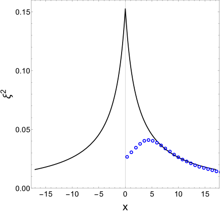
Figure 15: (Color online) The line corresponds to $\xi^{2}$ from Eq. (46) as a function of $x$ in the assumption of constant magnetization. Open points correspond to assumption used in the main text, of constant external current $\tilde{J}=1/100$.

Appendix D Alternative treatments of the effective potential away from the critical line

As we have seen above, the interrelation between the binary and many-body forces strongly depends on the magnitude of the correlation length $\xi$, which enters in large and different powers in the different diagrams. Mapping of the Ising variables to QCD phase diagram is a nontrivial problem, discussed in Refs. Stephanov (2011); Nonaka and Asakawa (2005).

In the main text we followed a simplified procedure to calculate the deformed potential, assuming certain $constant$ ($t$-independent) value of the external current $J$. It included calculation of the dependence of the magnetization (called there $\phi_{0}$) on $t$.

Here we would like to compare it to another simple map, assuming instead $\phi_{0}=M=const(t)$ and using epsilon expansion expression (46). The complicated function is used as a function of variable

$$x={|t|\over|M|^{1/\beta}}$$

The correlation length squared following from it is shown in Fig. 15 by a line, compared to the coefficient of $\delta^{2}$ term in those potentials, presented by open points. It shows that while two alternative assumptions agree at larger $t$, they produce very different values of the correlation length very close to the critical point. Deformation of the potential by $\tilde{J}=1/100$ imposes a stronger limit on the correlation length.

References

- Stephanov et al. (1998) M. A. Stephanov, K. Rajagopal, and E. V. Shuryak, Phys. Rev. Lett. 81, 4816 (1998), arXiv:hep-ph/9806219 [hep-ph] .
- Staig and Shuryak (2011) P. Staig and E. Shuryak, Phys. Rev. C 84, 034908 (2011), arXiv:1008.3139 [nucl-th] .
- Lacey et al. (2013) R. A. Lacey, Y. Gu, X. Gong, D. Reynolds, N. Ajitanand, J. Alexander, A. Mwai, and A. Taranenko, (2013), arXiv:1301.0165 [nucl-ex] .
- Shuryak and Torres-Rincon (2019) E. Shuryak and J. M. Torres-Rincon, Phys. Rev. C100, 024903 (2019), arXiv:1805.04444 [hep-ph] .
- Shuryak and Torres-Rincon (2020a) E. Shuryak and J. M. Torres-Rincon, Phys. Rev. C101, 034914 (2020a), arXiv:1910.08119 [nucl-th] .
- Stephanov (2011) M. A. Stephanov, Phys. Rev. Lett. 107, 052301 (2011), arXiv:1104.1627 [hep-ph] .
- DeMartini and Shuryak (2020) D. DeMartini and E. Shuryak, (2020), arXiv:2007.04863 [nucl-th] .
- Shuryak (2006) E. Shuryak, Critical point and onset of deconfinement. Proceedings, 3rd Conference, CPOD2006, Florence, Itlay, July 3-6, 2006, PoS CPOD2006, 026 (2006), arXiv:nucl-th/0609011 [nucl-th] .
- Berges et al. (2002) J. Berges, N. Tetradis, and C. Wetterich, Phys. Rept. 363, 223 (2002), arXiv:hep-ph/0005122 .
- Dupuis et al. (2020) N. Dupuis, L. Canet, A. Eichhorn, W. Metzner, J. Pawlowski, M. Tissier, and N. Wschebor, (2020), arXiv:2006.04853 [cond-mat.stat-mech] .
- Tsypin (1994) M. M. Tsypin, (1994), arXiv:hep-lat/9401034 [hep-lat] .
- Nonaka and Asakawa (2005) C. Nonaka and M. Asakawa, Phys. Rev. C71, 044904 (2005), arXiv:nucl-th/0410078 [nucl-th] .
- Adamczewski-Musch et al. (2020) J. Adamczewski-Musch et al. (HADES), Phys. Rev. C 102, 024914 (2020), arXiv:2002.08701 [nucl-ex] .
- Adam et al. (2020) J. Adam et al. (STAR), (2020), arXiv:2001.02852 [nucl-ex] .
- Shuryak and Torres-Rincon (2020b) E. Shuryak and J. M. Torres-Rincon, (2020b), arXiv:2005.14216 [nucl-th] .
- Zhao et al. (2020) W. Zhao, C. Shen, C. M. Ko, Q. Liu, and H. Song, Phys. Rev. C 102, 044912 (2020), arXiv:2009.06959 [nucl-th] .
- E. Brezin and Zinn-Justin (1976) J. C. L. G. E. Brezin and J. Zinn-Justin, in Phase Transition and Critical Phenomena, Vol. 6, edited by C. Domb and M. S. Green (Academic Press, New York, 1976).