InstaHide: Instance-hiding Schemes for Private Distributed Learning

How can multiple distributed entities collaboratively train a shared deep net on their private data while preserving privacy? This paper introduces InstaHide, a simple encryption of training images, which can be plugged into existing distributed deep learning pipelines. The encryption is efficient and applying it during training has minor effect on test accuracy.

InstaHide encrypts each training image with a “one-time secret key” which consists of mixing a number of randomly chosen images and applying a random pixel-wise mask. Other contributions of this paper include: (a) Using a large public dataset (e.g. ImageNet) for mixing during its encryption, which improves security. (b) Experimental results to show effectiveness in preserving privacy against known attacks with only minor effects on accuracy. (c) Theoretical analysis showing that successfully attacking privacy requires attackers to solve a difficult computational problem. (d) Demonstrating that use of the pixel-wise mask is important for security, since Mixup alone is shown to be insecure to some some efficient attacks. (e) Release of a challenge dataset to encourage new attacks. Our code is available at https://github.com/Hazelsuko07/InstaHide.

1 Introduction

In many applications, multiple parties or clients with sensitive data want to collaboratively train a neural network. For instance, hospitals may wish to train a model on their patient data. However, aggregating data to a central server may violate regulations such as Health Insurance Portability and Accountability Act (HIPAA) [Act96] and General Data Protection Regulation (GDPR) [VVdB18].

Federated learning [MMR⁺17, KMY⁺16] proposes letting participants train on their own data in a distributed fashion and share only model updates —i.e., gradients—with the central server. The server aggregates these updates (typically by averaging) to improve a global model and then sends updates to participants. This process runs iteratively until the global model converges. Merging information from individual data points into aggregated gradients intuitively preserves privacy to some degree. On top of that, it is possible to add noise to gradients in accordance with Differential Privacy (DP) [DKM⁺06, DR14], though careful calculations are needed to compute the amount of noise to be added [ACG⁺16, PCS⁺19]. However, the privacy guarantee of DP only applies to the trained model (i.e., approved use of data) and does not apply to side-channel computations performed by curious/malicious parties who are privy to the communicated gradients. Recent work [ZLH19] suggests that eavesdropping attackers can recover private inputs from shared model updates, even when DP was used. A more serious issue with DP is that meaningful guarantees involve adding so much noise that test accuracy reduces by over $20\%$ even on CIFAR-10 [PCS⁺19].

Cryptographic methods such as secure multiparty computation of [Yao82] and fully-homomorphic encryption [Gen09] can ensure privacy against arbitrary side-computations by adversary during training. Unfortunately it is a challenge to use them in modern deep learning settings, owing to their high computational overheads and their needs for special setups (e.g finite field arithmetic, public-key infrastructure).

Here we introduce a new method InstaHide, inspired by a weaker cryptographic idea of instance hiding schemes [AFK87]. We only apply it to image data in this paper and leave other data types (e.g., text) for future work. InstaHide gives a way to transform input $x$ to a hidden/encrypted input $\widetilde{x}$ in each epoch such that: (a) Training deep nets using the $\widetilde{x}$’s instead of $x$’s gives nets almost as good in terms of final accuracy; (b) Known methods for recovering information about $x$ out of $\widetilde{x}$ are computationally very expensive. In other words, $\widetilde{x}$ effectively hides information contained in $x$ except for its label.

InstaHide encryption has two key components. The first is inspired by Mixup data augmentation method [ZCDLP18], which trains deep nets on composite images created via linear combination of pairs of images (viewed as vectors of pixel values). In InstaHide the first step when encrypting image $x$ (see Figure 1) is to take its linear combination with $k-1$ randomly chosen images from either the participant’s private training set or from a large public dataset (e.g., ImageNet [DDS⁺09]). The second step of InstaHide involves applying a random pattern of sign flips on the pixel values of this composite image, yielding encrypted image $\widetilde{x}$, which can be used as-is in existing deep learning frameworks. Note that the set of random images for mixing and the random sign flipped mask are used only once —in other words, as a one-time key that is never re-used for another encryption.

The idea of random sign flipping is inspired by classic Instance-Hiding over finite field ${\sf GF}(2)$, which involves adding a random vector $r$ to an input $x$. (See Appendix A for background.) Adding $1$ over ${\sf GF}(2)$ is analogous to a sign flip over $\mathbb{R}$. (Specifically, the groups $({\sf GF}(2),+)$ and $(\{\pm 1\},\times)$ are isomorphic.) The use of a public dataset in InstaHide plays a role reminiscent of random oracle in cryptographic schemes [CGH04] —the larger this dataset, the better the conjectured security level (see Section 4). A large private dataset would suffice too for security, but then would require prior coordination/sharing among participants.

Figure 1: Applying InstaHide ($k=4$) to the leftmost private image consists of mixing with another (private) image randomly chosen from the training set and two images randomly chosen from a fixed large public dataset. This is followed by a random sign-flipping mask on the composite image. To encrypt another image, different random choices will get used (“one-time key”).

Experiments on MNIST, CIFAR-10, CIFAR-100 and ImageNet datasets (see Section 5) suggest that InstaHide is an effective approach to hide training images from attackers. It is much more effective at hiding images than Mixup alone and provides better trade-off between privacy preservation and accuracy than DP. To enable further rigorous study of attacks, we release a challenge dataset of images encrypted using InstaHide.

Enhanced functionality due to InstaHide.

As hinted above, InstaHide plugs seamlessly into existing distributed learning frameworks such as federated learning: clients encrypt their inputs on the fly with InstaHide and participate in training (without using DP). Depending upon the level of security needed in the application (see Section 4.1), InstaHide can also be used to present enhanced functionality that are unsafe in current distributed frameworks. For instance, in each epoch, computationally limited clients can encrypt each private input $x$ to $\widetilde{x}$ and ship it to the central server for all subsequent computation. The server may randomize in the pooled data to create its own batches to deal with special learning situations when distributed data are not independent and identically distributed.

Security goal of InstaHide.

The goal of InstaHide is to provide a light-weight encryption method to make it difficult for attackers to recover the training data in a large training dataset in a distributed learning setting, with minor reduction on data utility. It is not designed to provide the level of security strength as encryption methods such as RSA [RSA78]. It is an initial step towards exploring better privacy preservation while maintaining data utility.

Rest of the Paper:

Section 2 recaps Mixup and suggests it alone is not secure. Section 3 presents two InstaHide schemes, and Section 4 analyzes their security. Section 5 shows experiments for InstaHide’s efficiency, efficacy, and security. Section 6 provides suggestions for practical use, and Section 7 describes the challenge dataset. We review related work in Section 8, discuss potential attacks in Section 9 and conclude in Section 10.

2 Mixup and Its Vulnerability

This section reviews Mixup method [ZCDLP18] for data augmentation in deep learning and shows —using two plausible attacks— that it alone does not assure privacy. For ease of description, we consider a vision task with a private dataset $\mathcal{X}\subset\operatorname{{\mathbb{R}}}^{d}$ of size $n$. Each image $x_{i}\in\mathcal{X},i\in[n]$ is normalized such that $\sum_{j=1}^{d}x_{i,j}=0$ and $\|x_{i}\|_{2}=1$.

See Algorithm 1. Given an original dataset, in each epoch of the training the algorithm generates a Mixup dataset on the fly, by linearly combining $k$ random samples, as well as their labels (lines 9, 10). Mixup suggests that training with mixed samples and mixed labels serves the purpose of data augmentation, and achieves better test accuracy on normal images.

We describe the algorithm as an operation on $k$ images, but previous works mostly used $k=2$.

2.1 Attack on Mixup within a Private Dataset

We propose an attack to the Mixup method when a private image is mixed up more than once during training. In fact, in Algorithm 1, each image is used $kT$ times during training, where $k$ is the number of samples to mix, and $T$ is the number of training epochs.

Algorithm 1 Mixup [ZCDLP18]

1:procedure Mixup($W,T,\mathcal{X},\mathcal{Y}$)

2:    $W$: the weights of the deep neural network; $T$: number of epochs; ${\cal X}=\{x_{1},\cdots,x_{n}\},{\cal Y}=\{y_{1},\cdots,y_{n}\}$: the original dataset.

3:    Initialize $W$

4:    for $t=1\to T$ do

5:         Generate $\pi_{1}$ such that $\pi_{1}(i)=i$, $\forall i\in[n]$, and $k-1$ random permutations $\pi_{2}$, $\cdots$, $\pi_{k}:[n]\rightarrow[n]$ $\triangleright$ $[n]$ denotes $\{1,2,\cdots,n\}$

6:         Sample $\lambda_{1},\cdots,\lambda_{n}\sim[0,1]^{k}$ uniformly at random, and for all $i\in[n]$ normalize $\lambda_{i}$ such that $\|\lambda_{i}\|_{1}=1$.

7:         $\widetilde{D}\leftarrow\emptyset$

8:         for $i=1\to n$ do $\triangleright$ Generate Mixup dataset

9:             $\widetilde{x}_{i}^{\mathrm{mix}}\leftarrow\sum_{j=1}^{k}(\lambda_{i})_{j}\cdot x_{\pi_{j}(i)}$ $\triangleright$ Mix images

10:             $\widetilde{y}_{i}\leftarrow\sum_{j=1}^{k}(\lambda_{i})_{j}\cdot y_{\pi_{j}(i)}$ $\triangleright$ Mix labels

11:             $\widetilde{D}\leftarrow\widetilde{D}\cup(\widetilde{x}_{i},\widetilde{y}_{i})$

12:         end for

13:         Train $W$ using the Mixup dataset $\widetilde{D}$

14:    end for

15:end procedure

Assume that pairs of images in $\mathcal{X}$ are fairly independent at the pixel level, so that the inner product of a random pair of images (viewed as vectors) has expectation $0$ (expectation can be nonzero but small). We can think of each pixel is generated from some distribution with standard deviation $1/\sqrt{d}$ and describe attacks with this assumption. (Section 5 presents experiments showing that these attacks do work in practice.)

Suppose we have two Mixup images $\widetilde{x}_{1}$ and $\widetilde{x}_{2}$ which are derived from two subsets of private images, ${\mathcal{S}}_{1},{\mathcal{S}}_{2}\subset\mathcal{X}$ and $|{\mathcal{S}}_{1}|=|{\mathcal{S}}_{2}|=k$. If $\widetilde{x}_{1}$ and $\widetilde{x}_{2}$ contain different private images, namely ${\mathcal{S}}_{1}\cap{\mathcal{S}}_{2}=\emptyset$, then the expectation of $\widetilde{x}_{1}\cdot\widetilde{x}_{2}$ is 0. However, if ${\mathcal{S}}_{1}\cap{\mathcal{S}}_{2}\neq\emptyset$, and $\widetilde{x}_{1}$ and $\widetilde{x}_{2}$ have coefficients $\lambda_{1}$ and $\lambda_{2}$ for the common image in these two sets, then the expectation of $\langle\widetilde{x}_{1},\widetilde{x}_{2}\rangle$ is $\lambda_{1}\lambda_{2}/k$, which means by simply checking the inner products between two $\widetilde{x}$’s, the attacker can determine with high probability whether they are derived from the same image. Thus if the attacker finds multiple such pairs, they can average the $\widetilde{x}$’s to start getting a good estimate of $x$. (Note that the rest of images in the pairs are with high probability distinct and so average to $0$.)

2.2 Attack on Mixup Between a Private and a Public Dataset

To defend against the previous attack, it seems that a possible method is to modify the Mixup method to mix a private image $x$ with $k-1$ images only once to get a single $\widetilde{x}$, and use this $\widetilde{x}$ as surrogate for $x$ in all epochs. To ensure $x\in\mathcal{X}$ is used only once, it uses an additional public dataset $\mathcal{X^{\prime}}$ (e.g. ImageNet). In other words, for every $x\in\mathcal{X}$, it produces $\widetilde{x}$ by using Mixup between $x$ and $k-1$ random images from a large public dataset.

This extension of the Mixup method seems secure at first glance, as naively one can imagine that to violate privacy, the adversary must do exhaustive search over $(k-1)$-tuples of public images to determine which were mixed into $\widetilde{x}$, and try all possible $k$-tuples of coefficients, and then subtract the corresponding sum from $\widetilde{x}$ to extract $x$. If this is true, it would suggest that extracting $x$ or any approximation to it requires ${N\choose{k-1}}\approx N^{k-1}$ work, where $N$ is the number of images in the public dataset. This work becomes infeasible even for $k=4$. However, we sketch an attack below that runs in $O(Nk)$ time.

It again uses the above assumption about the pairwise independence property of a random image pair. Recall that standard deviation of pixels is $1/\sqrt{d}$. Namely, to determine the images that went into the mixed sample $\widetilde{x}=\lambda_{1}x_{1}+\sum_{i=2}^{k}\lambda_{i}x_{i}$, it suffices to go through each image $z$ in the dataset and examine the inner product $z\cdot\widetilde{x}$. If $z$ is not one of the $x_{i}$’s then this inner product is of the order at most $\sqrt{k/d}$ (see part 1 of Theorem B.3), whereas if it is one of the $x_{i}$’s then it is of the order at least $\frac{1}{k}(1-\sqrt{k/d})$ (see part 2 of Theorem B.3). Thus if $k^{3}\ll d$ (which is true if the number of pixels $d$ is a few thousand) then the inner product gives a strong signal whether $z$ is one of the $x_{i}$’s. Once the correct $x_{i}$’s and their coefficients have been guessed, we obtain $x$ up to a linear scaling. Thus the above attack works with good probability and in time proportional to the size of the dataset. We provide results for this attack in Section 5.

This attack of course requires that $x$ is being mixed in with images from a public dataset $\mathcal{X^{\prime}}$. In the case that $\mathcal{X^{\prime}}$ is private and diverse enough, it is conceivable that Mixup is safe. (MNIST for example may not be diverse enough but ImageNet probably is.) We leave it as an open question.

2.3 Discussions

Setting	Secure?
$x$ is mixed in multiple $\widetilde{x}$’s	No
$x$ is mixed in a single $\widetilde{x}$, with a public dataset	No
$x$ is mixed in a single $\widetilde{x}$, with a private dataset	Maybe

Table 1: Security of Mixup alone.

Table 1 summarizes the security of Mixup . Only Mixup with single $\widetilde{x}$ for each private $x$ and within a private dataset(s) has not been identified vulnerable to potential attacks. But this does not necessarily mean it is secure. In addition, the test accuracy in this case is not comparable to vanilla training; it incurs about $20\%$ accuracy loss with CIFAR-10 tasks.

Potentially insecure applications of Mixup.

Recently, a method called FaceMix  [LWZ⁺19] applies Mixup at the representation level (i.e. intermediate output of deep models) during inference. Given a representation function $h:\operatorname{{\mathbb{R}}}^{d}\rightarrow\operatorname{{\mathbb{R}}}^{l}$ and a secret $x\in\operatorname{{\mathbb{R}}}^{d}$, the paper assumed a threat model that the attacker is able to reconstruct $x$ given $h(x)$. Therefore, FaceMix proposed to protect the privacy of $x$ by generating $\widetilde{h}_{1}(x)=\lambda_{1}h(x)+\sum_{i=2}^{k}\lambda_{i}h(x_{i})$, and run inference on $\widetilde{h}(x)$. A similar but different idea was shown in [FWX⁺19], which proposed to generate $\widetilde{x}=\lambda_{1}x+\sum_{i=2}^{k}\lambda_{i}x_{i}$ and use $\widetilde{h}_{2}(x)=h(\widetilde{x})$ for training.

Both methods may be vulnerable to the attacks presented in this section: when $h$ is linear (one example in [LWZ⁺19]), we have $\widetilde{h}_{1}(x)=\widetilde{h}_{2}(x)$, which means the attacker can reconstruct the Mixup image $\widetilde{x}=\lambda_{1}x+\sum_{i=1}^{k}x_{i}$ from $\widetilde{h}_{1}(x)$ and run attacks on Mixup. For a nonlinear $h$, $\widetilde{h}_{1}(x)\approx\widetilde{h}_{2}(x)$ may also hold.

3 InstaHide

This section first presents two schemes: Inside-dataset InstaHide and Cross-dataset InstaHide, and then describes their inference.

The Inside-dataset InstaHide mixes each training image with random images within the same private training dataset. The cross-dataset InstaHide, arguably more secure (see Section 4), involves mixing with random images from a large public dataset like ImageNet.

3.1 Inside-Dataset InstaHide

Algorithm 2 shows Inside-dataset InstaHide. Its encryption step includes mixing the secret image $x$ with $k-1$ other training images followed by an extra random pixel-wise sign-flipping mask on the composite image. Note that random sign flipping changes the color of a pixel. The motivation for random sign flips was described around Footnote 2.

Definition 3.1 (random mask distribution $\Lambda_{\pm}^{d}$).

Let $\Lambda_{\pm}^{d}$ denote the $d$-dimensional random sign distribution such that $\forall\sigma\sim\Lambda_{\pm}^{d}$, for $i\in[d]$, $\sigma_{i}$ is independently chosen from $\{\pm 1\}$ with probability 1/2 each.

Algorithm 2 Inside-dataset InstaHide

1:procedure InstaHide($W,T,\mathcal{X},\mathcal{Y}$) $\triangleright$ This paper

2:    $W$: weights of the neural network; $T$: number of epochs;
${\cal X}=\{x_{1},\cdots,x_{n}\}$: data; ${\cal Y}=\{y_{1},\cdots,y_{n}\}$: labels.

3:    Initialize $W$

4:    for $t=1\to T$ do

5:         Generate $\pi_{1}$ such that $\pi_{1}(i)=i$, $\forall i\in[n]$, and $k-1$ random permutations $\pi_{2}$, $\cdots$, $\pi_{k}:[n]\rightarrow[n]$

6:         Sample $\lambda_{1},\cdots,\lambda_{n}\sim[0,1]^{k}$ uniformly at random, and for all $i\in[n]$ normalize $\lambda_{i}\in\operatorname{{\mathbb{R}}}^{k}$ such that $\|\lambda_{i}\|_{1}=1$ and $\|\lambda_{i}\|_{\infty}\leq c_{1}$. $\triangleright$ $c_{1}\in[0,1]$ is a constant that upper bounds a single coefficient

7:         Sample $\sigma_{1},\cdots,\sigma_{n}\sim\Lambda_{\pm}^{d}$ uniformly at random. $\triangleright$ Definition 3.1

8:         $\widetilde{D}\leftarrow\emptyset$

9:         for $i=1\to n$ do $\triangleright$ Generate InstaHide dataset

10:             $\widetilde{x}_{i}\leftarrow\sigma_{i}\circ\sum_{j=1}^{k}(\lambda_{i})_{j}\cdot x_{\pi_{j}(i)}$ $\triangleright$ Encryption

11:             $\widetilde{y}_{i}\leftarrow\sum_{j=1}^{k}(\lambda_{i})_{j}\cdot y_{\pi_{j}(i)}$ $\triangleright$ Mix labels

12:             $\widetilde{D}\leftarrow\widetilde{D}\cup(\widetilde{x}_{i},\widetilde{y}_{i})$

13:         end for

14:         Train $W$ using the InstaHide dataset $\widetilde{D}$

15:    end for

16:end procedure

To encrypt a private input $x_{i}$, we first determine the random coefficient $\lambda$’s for image-wise combination, but with the constraint that they are at most $c_{1}$ to avoid dominant leakage of any single image (line 6 in Algorithm 2). Then we sample a random mask $\sigma_{i}\sim\Lambda_{\pm}^{d}$ and apply $\sigma\circ x$, where $\circ$ is coordinate-wise multiplication of vectors (line 10 in Algorithm 2). Note that the random mask $\sigma_{i}$ and the $k-1$ images used for mixing with $x_{i}$, will not be reused to encrypt other images. They constitute a “random one-time private key.”

A priori.

It may seem that using a different mask for each training sample would completely destroy the accuracy of the trained net, but as we will see later it has only a small effect when $k$ is small. Mathematically, this seems reminiscent of the phase retrieval problem [CSV13, LN18] (see Appendix D).

3.2 Cross-Dataset InstaHide

Cross-dataset InstaHide extends the encryption step of Algorithm 2 by mixing $k$ images from the private training dataset $D_{\text{private}}$ and a public dataset $D_{\text{public}}$, and a random mask as a random one-time secret key.

Although the second dataset can be private, there are several motivations to use a public dataset: (a) Some privacy-sensitive datasets, (e.g. CT or MRI scans), feature images with certain structure patterns with uniform backgrounds. Mixing among such images as in Algorithm 2 would not hide information effectively. (b) Drawing mixing images from a larger dataset gives greater unpredictability, hence better security (see Section 4). (c) Public datasets are freely available and eliminate the need for special setups among participants in a distributed learning setting.

To mix $k$ images in the encryption step, we randomly choose $2$ images from $D_{\text{private}}$ and the other $k-2$ from $D_{\text{public}}$, and apply InstaHide to all these images. The only difference in the cross-dataset scheme is that, the model is trained to learn only the (mixed) label of $D_{\text{private}}$ images. We assume $D_{\text{public}}$ images are unlabelled. For better accuracy, we lower bound the sum of coefficients of two private images by a constant $c_{2}\in[0,1]$.

We advocate preprocessing a public dataset in two steps to obtain $D_{\text{public}}$ for better security. The first is to randomly crop a number of patches from each image in the public dataset to form $D_{\text{public}}$. This step will make $D_{\text{public}}$ much larger than the original public dataset. The second is to filter out the “flat” patches. In our implementation, we design a filter using SIFT [Low99], a feature extraction technique to retain patches with more than 40 key points.

3.3 Inference with InstaHide

Either scheme above by default applies InstaHide during inference, by averaging predictions of multiple encryptions (e.g. 10) of a test sample. This idea is akin to existing cryptographic frameworks for secure evaluation on a public server via homomorphic encryption (e.g. [MLS⁺20]). Since the encryption step of InstaHide is very efficient, the overhead of such inference is quite small.

One can also choose not to apply InstaHide during inference. We found in our experiments (Section 5) that it works for low-resolution image datasets such as CIFAR-10 but it does not work well with a high-resolution image dataset such as ImageNet.

4 Security Analysis

This section considers the security of InstaHide in distributed learning, specifically the cross-dataset version.

Attack scenario: In each epoch, all clients replace each (image, label)-pair $(x,y)$ in the training set with some $(\widetilde{x},\widetilde{y})$ using InstaHide. Attackers observe $h(\widetilde{x},\widetilde{y})$ for some function $h$: in federated learning $h$ could involve batch gradients or hidden-layer activations computed using input $\widetilde{x},\widetilde{y}$ as well as other inputs.

Argument for security consists of two halves: (1) To recover significant information about an image $x$ from communicated information, computationally limited eavesdroppers/attackers have to break InstaHide encryption (Section 4.1). (2) Breaking InstaHide is difficult (Section 4.2).

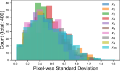
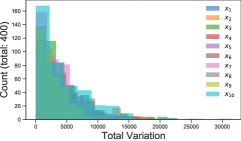
(a)

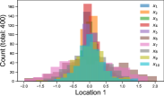
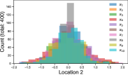
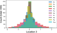
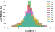
(b)

Figure 2: Empirical distributions of 3 statistics (first row) and 4 random locations (second row) for 400 InstaHide encryptions of 10 different images (cross-dataset, $k=4$). Distributions of encryptions of different images are indistinguishable.

4.1 Secure Encryption Implies Secure Protocol

Suppose an attacker exists that compromises an image $x$ in the protocol. We do the thought experiment of even providing the attacker with encryptions of all images belonging to all parties, as well as model parameters in each iteration. Now everything the attacker sees during the protocol it can efficiently compute by itself, and we can convert the attacker to one that, given $\widetilde{x}$, extracts information about $x$. We conclude in this thought experiment that a successful attack on the protocol also yields a successful attack on the encryption. In other words, privacy loss during protocol is upper bounded by privacy loss due to the encryption itself. Of course, this proof allows the possibility that the protocol —due to aggregation of gradients, etc.—ensures even greater privacy than the encryption alone.

Dealing with multiple encryptions of same $x$:

In our protocol each image $x$ is re-encrypted in each epoch. This seems to act as a data augmentation and improves accuracy. The above argument translated to this setting shows that privacy violation requires solving the following problem: private images $x_{1},x_{2},\ldots,x_{n}$ were each encrypted $T$ times ($n$ is size of the private training set, $T$ is number of epochs), each time using a new private key. Attacker is given these $nT$ encryptions. Weaker task: Attacker has to identify which of them came from $x_{1}$. Stronger task: Attacker has to identify $x_{1}$.

We conjecture both tasks are hard. Visualization (see Figure 2) as well as the Kolmogorov–Smirnov test [Kol33, Smi48] (see Appendix E) suggest that statistically, it is difficult to distinguish among distributions of encryptions of different images. Thus, effectively identifying multiple $\widetilde{x}$’s of same $x$ and using them to run attacks seems difficult.

4.2 Hardness of Attacking InstaHide Encryption

Now we consider the difficulty of recovering information about $x$ given a single encryption $\widetilde{x}$.

Security estimates of naive attack.

We start by considering the naive attack on cross-dataset InstaHide, which would involve the attacker to either figure out the set of all $k-2$ public images, or to compromise the mask $\sigma$ and run attacks on Mixup. This should take $\min\{|\mathcal{D}_{\rm public}|^{k-2},2^{d}\}$ time. For cross-dataset InstaHide schemes with a large public dataset (e.g. ImageNet), the computation cost of attack will be $10^{7(k-2)}$, and $k=4$ already makes the attack hard.

Now we suggest reasons why the naive attack may be best possible.

For worst-case pixel-vectors, finding the $k$-image set is hard.

Appendix C shows that for worst-case choices of images (i.e., when an “image” is allowed to be an arbitrary sequence of pixel values) the computational complexity of this problem is related to the famous $k$-vector subset sum problem. The attacker would need to exhaustively search over all possible combinations of public images, which is at the cost of $|\mathcal{D}_{\rm public}|^{k-2}$. Thus when $\mathcal{D}_{\rm public}$ is a large public dataset and $k\geq 4$, the computational effort to recover the image ought to be of the order of $10^{10}$ or more.

Of course, images are not worst-case vectors. Thus an attack must leverage this fact somehow. The obvious idea today is to use a deep net for the attack, and the experiments below will suggest the obvious ideas do not work.

Compromising the mask is also hard.

As previously discussed, the pixel-wise mask $\sigma\sim\Lambda_{\pm}^{d}$ ( Def. 3.1) in InstaHide is kept private by each client, which is analogous to a private key (assuming the client never shares its own $\sigma$ with others, and the generation of $\sigma$ is statistically random). Brute-force algorithm consumes $2^{d}$ time to figure out $\sigma$, where $d$ can be several thousands in vision tasks.

5 Experiments

We have conducted experiments to answer three questions:

1. How much accuracy loss does InstaHide suffer (Section 5.1)?

2. How is the accuracy loss of InstaHide compared to differential privacy approaches (Section 5.2)?

3. Can InstaHide defend against known attacks (Section 5.3)?

We are particularly interested in the cases where $k\geq 4$.

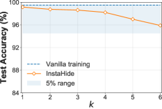
(a) MNIST

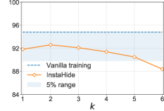
(b) CIFAR-10

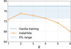
(c) CIFAR-100

Figure 3: Test accuracy ($\%$) on MNIST, CIFAR-10 and CIFAR-100 for vanilla training and inside-dataset InstaHide with different $k$’s. InstaHide with $k\leq 4$ only suffers small accuracy loss.

	MNIST	CIFAR-10	CIFAR-100	ImageNet	Assumptions
Vanilla training	$99.5\pm 0.1$	$94.8\pm 0.1$	$77.9\pm 0.2$	$77.4$	-
DPSGD∗	$98.1$	$72.0$	N/A	N/A	A1
InstaHide${}_{\text{\rm inside},k=4,\text{ \rm in inference}}$	$98.2\pm 0.2$	$91.4\pm 0.2$	$73.2\pm 0.2$	$72.6$	-
InstaHide${}_{\text{\rm inside},k=4}$	$98.2\pm 0.3$	$91.2\pm 0.2$	$73.1\pm 0.3$	1.4	-
InstaHide${}_{\text{\rm cross},k=4,\text{ \rm in inference}}$	$98.1\pm 0.2$	$90.3\pm 0.2$	$72.8\pm 0.3$	-	A2
InstaHide${}_{\text{\rm cross},k=4}$	$97.8\pm 0.2$	$90.7\pm 0.2$	$73.2\pm 0.2$	-	A2
InstaHide${}_{\text{\rm cross},k=6,\text{ \rm in inference}}$	$97.4\pm 0.2$	$89.6\pm 0.3$	$72.1\pm 0.2$	-	A2
InstaHide${}_{\text{\rm cross},k=6}$	$97.3\pm 0.1$	$89.8\pm 0.3$	$71.9\pm 0.3$	-	A2

Table 2: Test accuracy ($\%$) on MNIST, CIFAR-10, CIFAR-100 and ImageNet for vanilla training, DPSGD [ACG⁺16] and InstaHide, including the mean and standard deviation of test accuracy across 5 runs except for ImageNet. Results marked with “in inference” applies InstaHide during inference. InstaHide methods incur minor accuracy reductions. A1 denotes “Using a labelled public dataset for pre-training”, A2 denotes “ Using a large unlabelled public dataset for hiding”. ^∗DPSGD results are from [PCS⁺19], which does not have results for CIFAR-100 and ImageNet.

(a) Accuracy with different $\alpha$’s.

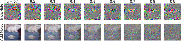
(b) Images generated by InstaHide and adding Laplace noise with different $\alpha$’s.

Figure 4: Relative accuracy on CIFAR-10 (a) and visualization (b) of InstaHide and adding random Laplace noise with different $\alpha$’s, the coefficient of perturbation. InstaHide gives better test accuracy than adding random noise.

Datasets and setup.

Our main experiments are image classification tasks on four datasets MNIST [LCB10], CIFAR-10, CIFAR-100 [Kri09], and ImageNet [DDS⁺09]. We use ResNet-18 [HZRS16] architecture for MNIST and CIFAR-10, NasNet [ZVSL18] for CIFAR-100, and ResNeXt-50 [XGD⁺17] for ImageNet. The implementation uses the Pytorch [PGM⁺19] framework. Note that we convert greyscale MNIST images to be 3-channel RGB images in our experiments. Hyper-parameters are provided in Appendix E.

5.1 Accuracy Results of InstaHide

We evaluate the following InstaHide variants (with $c_{1}=0.65,c_{2}=0.3$):

• Inside-dataset InstaHide with different $k$’s, where $k$ is chosen from $\{1,2,3,4,5,6\}$.

• Cross-dataset InstaHide with $k=4,6$. For MNIST, we use CIFAR-10 as the public dataset; for CIFAR-10 and CIFAR-100, we use the preprocessed ImageNet as the public dataset. We do not test Cross-dataset InstaHide on ImageNet since its sample size is already large enough for good security.

The computation overhead of InstaHide in terms of extra training time in our experiments is smaller than $5\%$.

Accuracy with different $k$’s.

Figure 3 shows the test accuracy of vanilla training, and inside-dataset InstaHide with different $k$’s on MNIST, CIFAR-10 and CIFAR-100 benchmarks. Compared with vanilla training, InstaHide with $k=4$ only suffers small accuracy loss of $1.3\%$, $3.4\%$, and $4.7\%$ respectively. Also, increasing $k$ from 1 (i.e., apply mask on original images, no Mixup) to 2 (i.e., apply mask on pairwise mixed images) improves the test accuracy for CIFAR datasets, suggesting that Mixup data augmentation also helps for encrypted InstaHide data points.

Inside-dataset v.s. Cross-dataset.

We also evaluate the performance of Cross-dataset InstaHide, which does encryption using random images from both the private dataset and a large public dataset. As shown in Table 2, Cross-dataset InstaHide incurs an additional small accuracy loss comparing with inside-dataset InstaHide. The total accuracy losses for MNIST, CIFAR-10 and CIFAR-100 are $1.7\%$, $4.1\%$, and $4.7\%$ respectively. As previously suggested, a large public dataset provides a stronger notion of security.

Inference with and without InstaHide.

As mentioned in Sec 3.3, by default, InstaHide is applied during inference. In our experiments, we average predictions of 10 encryptions of a test image. We found that for high-resolution images, applying InstaHide during inference is important: the results of using Inside-dataset InstaHide on ImageNet in Table 2 show that the accuracy of inference with InstaHide is $72.6\%$, whereas that without InstaHide is only $1.4\%$.

5.2 InstaHide vs. Differential Privacy approaches

Although InstaHide is qualitatively different from differential privacy in terms of privacy guarantee, we would like to provide hints for their relative accuracy (Question 2).

Comparison with DPSGD.

DPSGD [ACG⁺16] injects noise to gradients to control private leakage. Table 2 shows that DPSGD leads to an accuracy drop of about $20\%$ on CIFAR-10 dataset. By contrast, InstaHide gives models almost as good as vanilla training in terms of test accuracy.

Comparison with adding random noise to images.

We also compare InstaHide (i.e., adding structured noise) with adding random noise to images (another typical approach to preserve differential privacy). Specifically, given the original dataset $\mathcal{X}$, and a perturbation coefficient $\alpha\in(0,1)$, we test a) InstaHide_inside,k=2: $\widetilde{x}_{i}=\sigma\circ((1-\alpha)x_{i}+\alpha x_{j})$, where $x_{j}\in\mathcal{X}$, $j\neq i$, and b) adding random Laplace noise $e$: $\widetilde{x}_{i}=(1-\alpha)x_{i}+e$, where $\operatorname*{{\mathbb{E}}}[\|e\|_{1}]=\operatorname*{{\mathbb{E}}}[\|\alpha x_{j}\|_{1}]$.

As shown in Figure 4, by increasing $\alpha$ from 0.1 to 0.9, the test accuracy of adding random noise drops from $\sim 94\%$ to $\sim 10\%$, while the accuracy of InstaHide is above $90\%$.

5.3 Robustness Against Attacks

To answer the question how well InstaHide can defend known attacks, here we report our findings with a sequence of attacks on InstaHide encryption $\widetilde{x}$ to recover original image $x$, including gradient-matching attack [ZLH19], demasking using GAN (Generative Adversarial Network), averaging multiple encryptions, and uncovering public images with similarity search.

Gradient-matching attack [ZLH19].

Here attacker observes gradients of the loss generated using a user’s private image $s$ while training a deep net (attacker knows the deep net, e.g., as a participant in Federated Learning) and tries to recover $s$ by computing an image $s^{*}$ that has similar gradients to those of $s$ (see algorithm in Appendix E). Figure 5 shows results of this attack on Mixup and InstaHide schemes on CIFAR-10. If Mixup with $k=4$ is used, the attacker can still extract fair bit of information about the original image. However, if InstaHide is used the attack isn’t successful.

Demask using GAN.

InstaHide does pixel-wise random sign-flip after applying Mixup (with public images, in the most secure version). This flips the signs of half the pixels in the mixed image. An alternative way to think about it is that the adversary sees the intensity information (i.e. absolute value) but not the sign of the pixel. Attackers could use computer vision ideas to recover the sign. One attack consists of training a GAN on this sign-recovery task, using a large training set of $(z,\sigma\circ z)$ where $z$ is a mixed image and $\sigma$ is a random mask. If this GAN recovers the signs reliably, this effectively removes the mask, after which one could use the attacks against Mixup described in Section 2.

In experiments this only succeeded in recovering half the flipped signs, which means $\sim 1/4$ of the coordinates continued to have the wrong sign; see Figure 6. GAN training used 50,000 cross-dataset InstaHide examples generated with CIFAR-10 and ImageNet ($k=6$). This level of sign recovery seems insufficient to allow the attack against Mixup (Section 2) to succeed, nor the other attacks discussed below. Nevertheless, researchers trying to break InstaHide may want to use such a demasking GAN as a starting point.

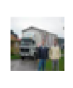
(a) Original

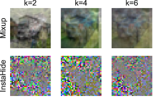
(b) After mixing

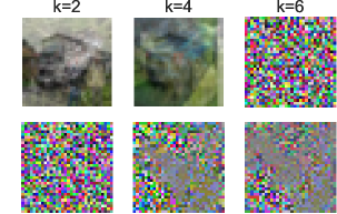
(c) Recovered by attack

Figure 5: Visualization of (a) the original image, (b) Mixup and InstaHide images, and (c) images recovered by the gradients matching attack. InstaHide is more effective in hiding the image than Mixup.

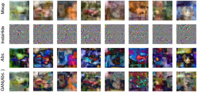
Figure 6: Undo sign-flipping using GAN. Rows: (1) Output from Mixup algorithm (Algorithm 1, line 9); (2) Result of applying random mask $\sigma$ on previous row (Algorithm 2, line 10). Note that randomly flipping sign of a pixel still preserves its absolute value. (3) Taking coordinate-wise absolute value of previous row. (4) Output of demasking GAN on previous row. The attack corrects about $1/4$ of the flipped signs but this doesn’t appear enough to allow further attacks that recover the encrypted image.

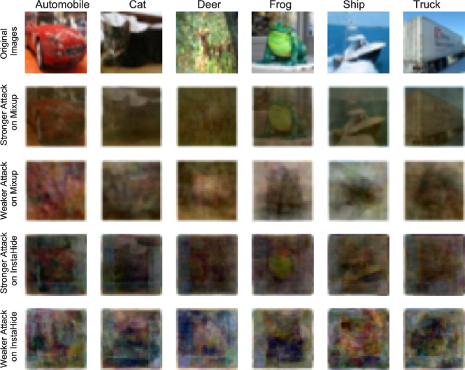
Figure 7: Average multiple encryptions (after demasking) of the same image to attack ($k=6$). In the stronger attack, the attacker already knows the set of multiple encryptions of the same image; in the weaker attack, the attacker has to identify that set first. Rows: (1) Original images. (2-3) Results of the stronger and the weaker attacks on Mixup. (4-5) Results of the stronger and the weaker attacks on InstaHide. Note that the attacker has to demask InstaHide encryptions using GAN before running attacks, and the information loss of this step makes it harder to attack InstaHide than the plain Mixup.

Average multiple encryptions of the same image.

We further test if different encryptions of the same image (after demasking) can be used to recover that hidden image by running the attack in Section 2.1.

Assuming a public history of $n\times T$ encryptions, where $n$ is the size of the private training set, and $T$ is the number of epochs. We consider a stronger and a weaker version of this attack.

• Stronger attack: the attacker already knows the set of multiple encryptions of the same image $x$. He uses GAN to demask all encryptions in the set, and averages images in the demasked set to estimate $x$.

• Weaker attack: the attacker does not know which subset of the encryption history correspond to the same original image. To identify that subset, he firstly demasks all $n\times T$ encrytions in the history using GAN. With an arbitrary demasked encryption (from the history) for some unknown original image $x$, he runs similarity search to find top-$m$ closest images in $n\times T-1$ other demasked encryptions (which may also contain $x$), and averages these $m+1$ images to estimate $x$.

The stronger attack is conceivable if $n$ is very small (say a hospital only has 100 images), so via brute force the attacker can effectively have a small set of encryptions of the same image. However, in practice, $n$ is usually at least a few thousand.

For simplicity, we test with $n=50$ and $T=50$ (a larger $n$ will make the attack harder). We use the structural similarity index measure (SSIM) [WBSS04] as the similarity metric, and set $m$ to 5 after tuning.

We also run this attack directly on Mixup for comparison. As shown in Figure 7, if the original image is not flat (e.g. the “deer”), the stronger attack may not work. For flat images (e.g. the “truck”) or images with strong contrast (e.g. the “automobile” and the “frog”), the stronger attack is able to vaguely recover the original image. However, as previously suggested, the stronger attack is feasible only for a very small $n$.

Note that results here is an upper bound on privacy leakage since we assume a perfect recovery of $\widetilde{x}$ from the gradients. In real-life scenarios this may not hold.

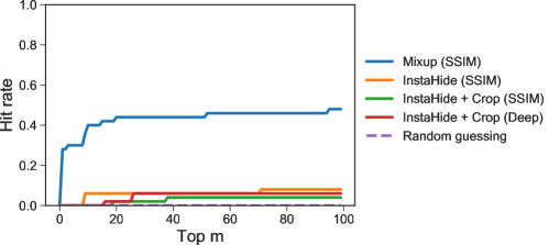
Figure 8: Averaged hit rate of uncovering public images for mixing among the top-$m$ answers returned by similarity search. Running this attack on InstaHide requires GAN-demasking as the first step, and a wrongly demasked pixel will make the similarity score less reliable and yield lower hit rate. Mixing with random cropped patches of public images augments the public dataset and gives more security. It also disables similarity search using SSIM. Train a deep model to predict similarity score also does not give a promising hit rate.

Uncover public images by similarity search.

We also run the attack in Section 2.2 after demasking InstaHide encryptions using GAN, which tries to uncover the public images for mixing by running similarity search in the public dataset using the demasked encryption as the query.

We test with $k=6$: mix 2 private images from CIFAR-10 with 4 public images from a set of 10,000 ImageNet images (i.e. $N=10,000$). We consider the attack a ‘hit’ if at least one public image for mixing is among the top-$m$ answers of the similarity search. The attacker uses SSIM as the default similarity metric for search. However, a traditional alignment-based similarity metric (e.g SSIM) would fail in InstaHide schemes which use randomly cropped patches of public images for mixing (see Figure 8), so in that case, the attacker trains a deep model (VGG [SZ15] in our experiments) to predict the similarity score.

Note that to find the 4 correct public images for mixing, the attack has to try all ${m\choose 4}$ combinations of the top-$m$ answers with different coefficients, and subtract the combined image from the demasked InstaHide encryption to verify. Figure 8 reports the averaged hit rate of this attack on 50 different InstaHide images. As shown, even with a relatively small public dataset ($N=10,000$) and a large $m=\sqrt{N}$, the hit rate of this attack on InstaHide (enhanced with random cropping) is around 0.05 (i.e. the attacker still has to try ${m\choose 4}=O(N^{2})$ combinations to succeed with probability 0.05). Also, this attack appears to become much more expensive with the public dataset being the whole ImageNet dataset ($N=1.4\times 10^{7}$) or random images on the Internet.

6 InstaHide Deployment: Best practice

Based on our security analysis (sec 4 and sec 5.3), we suggest the following:

• Consider Inside-dataset InstaHide only if the private dataset is very large and images have varied, complex patterns. If the images in the private dataset have simple signal patterns or the dataset size is relatively small, consider using Cross-dataset InstaHide.

• For Cross-dataset InstaHide, use a very large public dataset. Follow the preprocessing steps advocated in Sec 3.2 to randomly crop patches from each image in the public dataset and filter out “flat” patches.

• Re-encrypt images in each epoch. This allows the benefits of greater data augmentation for deep learning and hinders attacks (as suggested in Sec 5.3).

• Since images are re-encrypted in each epoch, for best security (e.g, against gradient-matching attacks), each participant should perform a random re-batching so that batch gradients do not correspond to the same subset of underlying images.

• Choose $k=4,5,6$ for a good trade-off between accuracy and security.

• Set a conservative upper threshold for the coefficients in mixing (e.g. $0.65$ in our experiments).

7 A Challenge Dataset

To encourage readers to design stronger attacks, we release a challenge dataset of encrypted images generated by applying Cross-dataset InstaHide with $k=6$ on some private image dataset and a preprocessed ImageNet as the public dataset. An attack is considered to succeed if it substantially recovers a significant fraction of original images.

8 Related Work

Mixup.

See Section 2. Mixup can improve both generalization and adversarial robustness [VLB⁺19]. It has also been adapted to various learning tasks, including semi-supervised data augmentation [BCG⁺19], unsupervised image synthesis [BHV⁺19], and adversarial defense at the inference stage [PXZ19]. Recently, [FWX⁺19] combined Mixup with model aggregation to defend against inversion attack, and [LWZ⁺19] proposed a novel method using Mixup for on-cloud privacy-preserving inference.

Differential privacy.

Differential privacy for deep learning involves controlling privacy leakage by adding noise to the learning pipeline. If the noise is drawn from certain distributions, say Gaussian or Laplace, it is possible to provide guarantees of privacy [DKM⁺06, DR14]. Applying differential privacy techniques to distributed deep learning is non-trivial. Shokri and Shmatikov [SS15] proposed a distributed learning scheme by directly adding noise to the shared gradients. However, the amount of privacy guaranteed drops with the number of training epochs and the size of shared parameters. DPSGD [ACG⁺16] was proposed to dynamically keep track of privacy spending based on the composition theorem [Dwo09]. However, it still leads to an accuracy drop of about $20\%$ on CIFAR-10 dataset. Also, to control privacy leakage, DPSGD has to start with a model pre-trained using nonprivate labeled data, and then carefully fine-tunes a few layers using private data.

Privacy using cryptographic protocols.

In distributed learning setting with multiple data participants, it is possible for the participants to jointly train a model over their private inputs by employing techniques like homomorphic encryption [Gen09, GLN12, LLH⁺17] or secure multi-party computation (MPC) [Yao82, Bei11, MZ17, DGL⁺19]. Recent work proposed to use cryptographic methods to secure federated learning by designing a secure gradients aggregation protocol [BIK⁺16] or encrypting gradients [AHWM17]. These approaches slow down the computation by orders of magnitude, and may also require special security environment setups.

Instance Hiding.

See Appendix A.

9 Discussions of Potential Attacks

We have received proposals of attacks since the release of early versions of this manuscript. We would like to thank these comments, which helped enhance the security of InstaHide. We hereby summarize some of them and explain why InstaHide in its current design is not vulnerable to them.

Tramèr’s attack.

Florian Tramèr [Tra20] suggested an attack pipeline which 1) firstly uses GANs to undo the random one-time sign flips of encrypted images, and 2) then runs standard image-similarity search between the recovered image and images in the public dataset.

We have evaluated this attack scenario in Section 5.3 (see ‘Demask using GAN’ for the first step, and ‘Uncover public images by similarity search’ for the second step). As shown, the GAN demasking step corrects about 1/4 of the flipped signs (see Figure 6), however this doesn’t appear enough to allow further attacks (see Figure 8).

Several designs of InstaHide could provide better practice of privacy under this attack: 1) setting a conservative upper threshold for the coefficients in mixing (e.g. 0.65 in our experiments) makes it harder to train the demasking GAN. 2) To alleviate the threat of image-similarity search for public image retrieval, we use randomly cropped patches from public images. This could enlarge the search space of pubic images by some large constant factor. We also suggest using a very large public dataset (e.g. ImageNet) if possible.

Braverman’s attack.

Mark Braverman [Bra20] proposed another possible attack to retrieve public images got mixed in an InstaHide image. Given $\widetilde{x}\in\operatorname{{\mathbb{R}}}^{d}$, the InstaHide image and the public dataset ${\cal D}\subset\operatorname{{\mathbb{R}}}^{d}$, the attacker calculates for each $s\in\cal D$ the value $v_{s}=\langle\widetilde{x}^{2},s^{2}\rangle-\frac{1}{d}\|\widetilde{x}\|_{2}^{2}\|s\|_{2}^{2}$, and ranks them in descending order. Braverman suggested that in theory, if images are drawn from Gaussian distributions, the public images got mixed will have higher ranks (i.e., there is a gap between $v_{s}$’s for $s$’s got mixed in $\widetilde{x}$ and $v_{s}$’s for $s$’s not got mixed in $\widetilde{x}$). With that, the attacker may be able to shrink the candidate search space for public images by a large factor. A brief accompanying paper with theory and experiments for this attack is forthcoming.

Braverman’s attack can be seen as similar in spirit to the attack on vanilla Mixup in Section 2.2, with the difference that it needs images to behave like Gaussian vectors for higher moments, and not just inner products. In the empirical study, we find 1) the gaussianity assumption is not so good for real images 2) the shrinkage of candidate search space by Braverman’s attack is small for $k=4$ and almost disappears for $k=6$.

To alleviate the risk of Bravermen’s attack, we reemphasize our suggestions in Section 6: 1) use a large public dataset and use random cropping as the preprocessing step. This will increase the original search space of public images; 2) use a larger $k$ (e.g. 6) if possible (3) maybe use a high quality GAN instead of the public dataset for mixing.

Carlini et al.’s attack.

Carlini et al. [CDG⁺20] gave an attack to recover private images in the most vulnerable application of InstaHide - when the InstaHide encryptions are revealed to the attacker. The first step is to train a neural network on a public dataset for similarity annotation to infer whether a pair of InstaHide encryptions contain the same private image. With the inferred similarities of all pairs of encryptions, the attacker then runs a combinatorial algorithm (cubic time in size of private dataset) to cluster all encryptions based on their original private images, and finally uses a regression algorithm to recover the private images.

Carlini et al.’s attack is able to give high-fidelity recoveries on our challenge dataset of 100 private images, but several limitations may prevent the current attack from working in a more realistic setting:

• The current attack runs in time cubic in the dataset size, and it can’t directly attack an individual encryption. Running time was not an issue for attacking our challenge set, which consisted of 5,000 encrypted images derived from 100 images. But feasibility on larger datasets becomes challenging.

• The challenge dataset corresponded to an ambitious form of security, where the encrypted images themselves are released to the world. The more typical application is a Federated Learning scenario where the attacker observes gradients computed using the inputs. When InstaHide is adopted in Federated Learning, the attacker only observes gradients computed on encrypted images. The attacks in this paper do not currently apply to that scenario. A possible attack to recover the original images may require recovering encrypted images from the gradients [ZLH19, GBDM20] as the first step.

10 Conclusion

InstaHide is a practical instance-hiding method for image data for private distributed deep learning.

InstaHide uses the Mixup method with a one-time secret key consisting of a pixel-wise random sign-flipping mask and samples from the same training dataset (Inside-dataset InstaHide) or a large public dataset (Cross-dataset InstaHide). The proposed method can be easily plugged into any existing distributed learning pipeline. It is very efficient and incurs minor reduction in accuracy. Maybe modifications of this idea can further alleviate the loss in accuracy that we observe, especially as $k$ increases.

We hope our analysis of InstaHide’s security on worst-case vectors will motivate further theoretical study, including for average-case settings and for adversarial robustness. In Appendix D, we suggest that although InstaHide can be formulated as a phase retrieval problem, classical techniques have failed as attacks.

We have tried statistical and computational attacks against InstaHide without success. To encourage other researchers to try new attacks, we release a challenge dataset of encrypted images.

Appendix

The appendix is organized as follows: Appendix A reviews Instance hiding. Appendix B provides more details for two attacks on Mixup schemes in Section 2. Appendix C discusses $k$-SUM, a well-known fine-grained complexity problem that is related to the worst-case security argument of InstaHide. Appendix D shows the connection between InstaHide and phase retrieval. Finally, Appendix E provides experimental details.

Appendix A Instance Hiding

In the classical setting of instance hiding [AFK87] in cryptography, a computationally-limited Alice is trying to get more powerful computing services Bob₁ and Bob₂ to help her compute a function $f$ on input $x$, without revealing $x$. The simplest case is that $f$ is a linear function over a finite field (e.g., integers modulo a prime number). Then Alice can pick a random number $r$ and “hide” the input $x$ by asking Bob₁ for $f(x+r)$ and Bob₂ for $f(r)$, and then infer $f(x)$ from the two answers. When all arithmetic is done modulo a prime, it can be shown that neither Bob₁ nor Bob₂ individually learns anything (information-theoretically speaking) about $x$. This scheme can also be applied to compute polynomials instead of linear functions.

InstaHide is inspired by the special case where there is a single computational agent Bob₁. Alice has to use random values $r$ such that she knows $f(r)$, and simply ask Bob₁ to supply $f(x+r)$. Note that such a random value $r$ would be use-once (also called nonce in cryptography); it would not be reused when trying to evaluate a different input.

Appendix B Attacks on Mixup

Here we provide more details for the attacks discussed in Section 2.

Notations.

We use $\langle u,v\rangle$ to denote the inner product between vector $u$ and $v$. We use $\mathbf{0}$ to denote the zero vector. For a vector $x$, we use $\|x\|_{2}$ to denote its $\ell_{2}$ norm. For a positive integer $n$, we use $[n]$ to denote set $\{1,2,\cdots,n\}$. We use $\Pr[]$ to denote the probability, use $\operatorname*{{\mathbb{E}}}[]$ to denote the expectation. We use ${\cal N}(\mu,\sigma^{2})$ to denote Gaussian distribution. For any two vectors $x,y$, we use $\langle x,y\rangle$ to denote the inner product.

B.1 Don’t mix up the same image multiple times

Let us continue with the vision task. This attack argues that given a pair of Mixup images $\widetilde{x}_{1}$ and $\widetilde{x}_{2}$, by simply checking $\langle\widetilde{x}_{1},\widetilde{x}_{2}\rangle$, the attacker can determine with high probability whether $\widetilde{x}_{1}$ and $\widetilde{x}_{2}$ are derived from the same image. We show this by a simple case with $k=2$ in Theorem B.1, where $k$ is the number of images used to generate a Mixup sample.

Theorem B.1.

Let $\mathcal{X}\subset\operatorname{{\mathbb{R}}}^{d}$ with $|{\cal X}|=n$ and $\forall x\in\mathcal{X},$ we sample $x\sim{\cal N}(0,\sigma^{2}I)$ where $\sigma^{2}=1/d$. Let $\mathcal{X}_{1}$, $\mathcal{X}_{2}$ and ${\mathcal{X}}_{3}$ denote three disjoint sets such that ${\mathcal{X}}_{1}\cup{\mathcal{X}}_{2}\cup{\mathcal{X}}_{3}=\mathcal{X}$, with probability $1-\delta$, we have:
Part 1. For $x_{1}\in{\cal X}_{1},x_{2},x_{2}^{\prime}\in{\cal X}_{2},x_{3}\in{\cal X}_{3}$, $\langle{x}_{3}+x_{1},{x}_{2}+x_{2}^{\prime}\rangle\leq c_{1}\cdot 4\sigma^{2}\sqrt{d}\log^{2}(dn/\delta)$.
Part 2. For $x_{1}\in{\cal X}_{1},x_{2}\in{\cal X}_{2},x_{3}\in{\cal X}_{3}$, $\langle{x}_{3}+{x}_{1},{x}_{3}+{x}_{2}\rangle\geq(c_{2}\cdot\sqrt{\log(n/\delta)}+d)\sigma^{2}-c_{1}\cdot 3\sigma^{2}\sqrt{d}\log^{2}(dn/\delta)$. where $c_{1},c_{2}>0$ are two universal constants.

Proof.

Part 1. First, we can expand $\langle{x}_{3}+x_{1},{x}_{2}+x_{2}^{\prime}\rangle$,

$$\langle{x}_{3}+x_{1},{x}_{2}+x_{2}^{\prime}\rangle =\langle{x}_{3},{x}_{2}\rangle+\langle{x}_{1},{x}_{2}\rangle+\langle{x}_{3},{x}_{2}^{\prime}\rangle+\langle{x}_{1},{x}_{2}^{\prime}\rangle$$

For each fixed $u\in\{x_{3},x_{1}\}$ and each fixed $v\in\{x_{2},x_{2}^{\prime}\}$, using Lemma B.8, we have

$$\Pr\Big{[}|\langle u,v\rangle|\geq c_{1}\cdot\sigma^{2}\sqrt{d}\log^{2}(dn/\delta)\Big{]}\leq\delta/n^{2}.$$

where $c_{1}>1$ is some sufficiently large constant.

Since $x_{1},x_{2},x_{2},x_{3}$ are independent random Gaussian vectors, taking a union bound over all pairs of $u$ and $v$, we have Lemma B.8, we have

$$\Pr[|\langle{x}_{3}+x_{1},{x}_{2}+x_{2}^{\prime}\rangle|\geq c_{1}\cdot 4\sigma^{2}\sqrt{d}\log^{2}(dn/\delta)\Big{]}\leq 4\delta/n^{2}.$$ (1)

Part 2.

We can lower bound $|\langle{x}_{3}+x_{1},{x}_{3}+x_{2}\rangle|$ in the following sense,

$$|\langle{x}_{3}+x_{1},{x}_{3}+x_{2}\rangle|= ~{}|\langle x_{3},x_{3}\rangle+\langle x_{3},x_{2}\rangle+\langle x_{1},x_{3}\rangle+\langle x_{1},x_{2}\rangle|$$

$$\geq ~{}|\langle x_{3},x_{3}\rangle|-|\langle x_{3},x_{2}\rangle+\langle x_{1},x_{3}\rangle+\langle x_{1},x_{2}\rangle|$$

For a fixed $x_{3}$, we can lower bound $\|x_{3}\|_{2}^{2}$ with Lemma B.5,

$$\Pr\Big{[}\|x_{3}\|_{2}^{2}>(c_{2}\cdot\sqrt{\log(n/\delta)}+d)\sigma^{2}\Big{]}\geq 1-\delta/n^{2}.$$

Since $x_{1},x_{2},x_{3}$ are independent random Gaussian vectors, using Lemma B.8, we have

$$\Pr[|\langle x_{3},x_{2}\rangle+\langle x_{1},x_{3}\rangle+\langle x_{1},x_{2}\rangle|\geq c_{1}\cdot 3\sigma^{2}\sqrt{d}\log^{2}(dn/\delta)\Big{]}\leq 3\delta/n^{2}.$$ (2)

where $c_{1}>1$ is some sufficiently large constant.

Thus, for a fixed $x_{3}$, we have

$$|\langle{x}_{3}+x_{1},{x}_{3}+x_{2}\rangle|\geq(c_{2}\cdot\sqrt{\log(n/\delta)}+d)\sigma^{2}-c_{1}\cdot 3\sigma^{2}\sqrt{d}\log^{2}(dn/\delta)$$

holds with probability $1-\delta/n^{2}-3\delta/n^{2}=1-4\delta/n^{2}$. ∎

Corollary B.2.

Let $\mathcal{X}\subset\operatorname{{\mathbb{R}}}^{d}$ with $|{\cal X}|=n$ and $\forall x\in\mathcal{X},$ we sample $x\sim{\cal N}(0,\sigma^{2}I)$ where $\sigma^{2}=1/d$. Let $\mathcal{X}_{1}$, $\mathcal{X}_{2}$ and ${\mathcal{X}}_{3}$ denote three disjoint sets such that ${\mathcal{X}}_{1}\cup{\mathcal{X}}_{2}\cup{\mathcal{X}}_{3}=\mathcal{X}$.
For any $\beta>1$, if $(2\beta)^{-1}\cdot\sqrt{d}\log^{2}(nd/\delta)\geq 4$, then with probability $1-\delta$ , we have :
for $x_{1}\in\mathcal{X}_{1},x_{2},x_{2}^{\prime}\in\mathcal{X}_{2},x_{3}\in\mathcal{X}_{3}$,

$$|\langle x_{3}+x_{1},x_{3}+x_{2}\rangle|\geq\beta\cdot|\langle x_{3}+x_{1},x_{2}+x_{2}^{\prime}\rangle|.$$

Proof.

With Theorem B.1, we have with probability $1-\delta$, we have :

$$\frac{|\langle x_{3}+x_{1},x_{3}+x_{2}\rangle|}{|\langle x_{3}+x_{1},x_{2}+x_{2}^{\prime}\rangle|}\geq ~{}\frac{(c_{2}\cdot\sqrt{\log(n/\delta)}+d)\sigma^{2}-c_{1}\cdot 3\sigma^{2}\sqrt{d}\log^{2}(dn/\delta)}{c_{1}\cdot 4\sigma^{2}\sqrt{d}\log^{2}(nd/\delta)}$$

$$= ~{}\frac{c_{2}\cdot\sqrt{\log(n/\delta)}+d-c_{1}\cdot 3\sqrt{d}\log^{2}(nd/\delta)}{c_{1}\cdot 4\sqrt{d}\log^{2}(nd/\delta)}$$

$$= ~{}\frac{1+c_{2}/(c_{1}\cdot d)\cdot\sqrt{\log(n/\delta)}-3/\sqrt{d}\cdot\log^{2}(nd/\delta)}{4/\sqrt{d}\cdot\log^{2}(nd/\delta)}$$

$$\geq ~{}\frac{1-3/\sqrt{d}\cdot\log^{2}(nd/\delta)}{4/\sqrt{d}\cdot\log^{2}(nd/\delta)}\geq~{}\frac{1-1/(2\beta)}{1/(2\beta)}=~{}2\beta-1\geq~{}\beta,$$

where the forth step follows from choice $c_{1}$ and $c_{2}$, the fifth step follows from assumption in Lemma statement, and the last step follows from $\beta>1$.

Thus, we complete the proof. ∎

B.2 Attacks that run in $|\mathcal{X}|$ time

This attack says that, if a cross-dataset Mixup sample $\widetilde{x}$ is generated by mixing 1 sample from a privacy-sensitive original dataset and $k-1$ samples from a public dataset (say ImageNet [DDS⁺09]), then the attacker can crack the $k-1$ samples from the public dataset by simply checking the inner product between $\widetilde{x}$ and all images in the public dataset. We show this formally in Theorem B.3.

Theorem B.3.

Let $\mathcal{X}\subset\operatorname{{\mathbb{R}}}^{d}$ with $|{\cal X}|=n$ and $\forall x\in\mathcal{X},$ we sample $x\sim{\cal N}(0,\sigma^{2}I)$. Let $\widetilde{x}=\sum_{i=1}^{k}x_{i}$, where $x_{i}\in\mathcal{X}$, with probability $1-\delta$, we have:
Part 1. For all $t^{\prime}\in[n]\backslash[k]$, $\langle\widetilde{x},x_{t^{\prime}}\rangle\leq c_{1}\cdot k\sigma^{2}\sqrt{d}\log^{2}(nd/\delta)$.
Part 2. For all $t\in[k]$, $\langle\widetilde{x},x_{t}\rangle\geq(c_{2}\cdot\sqrt{\log(n/\delta)}+d)\sigma^{2}-c_{1}\cdot(k-1)\sigma^{2}\sqrt{d}\log^{2}(nd/\delta)$.
where $c_{1},c_{2}>0$ are two universal constants.

We remark that the proof of Theorem B.3 is similar to the proof of Theorem B.1.

Proof.

Part 1. We can rewrite $\langle\widetilde{x},x_{t^{\prime}}\rangle$ as follows:

$$\langle\widetilde{x},x_{t^{\prime}}\rangle =\sum_{i=1}^{k}\langle{x}_{i},{x}_{t^{\prime}}\rangle,$$

which implies

$$|\langle\widetilde{x},x_{t^{\prime}}\rangle|\leq\sum_{i=1}^{k}|\langle{x}_{i},{x}_{t^{\prime}}\rangle|.$$

For each fixed $i\in[k]$ and each fixed $t^{\prime}\notin[k]$, using Lemma B.8, we have

$$\Pr\Big{[}|\langle x_{i},x_{t^{\prime}}\rangle|\geq c_{1}\cdot\sigma^{2}\sqrt{d}\log^{2}(dn/\delta)\Big{]}\leq\delta/n^{2}.$$

where $c_{1}>1$ is some sufficiently large constant.

Since $x_{1},x_{2},\cdots,x_{k},x_{t^{\prime}}$ are independent random Gaussian vectors, taking a union over all $i\in[k]$, we have

$$\Pr\Big{[}|\langle\widetilde{x},x_{t^{\prime}}\rangle|\geq c_{1}\cdot k\sigma^{2}\sqrt{d}\log^{2}(dn/\delta)\Big{]}\leq\delta k/n^{2}.$$

Taking a union bound over all $t^{\prime}\in[n]\backslash[k]$, we have

$$\Pr\Big{[}\forall t^{\prime}\in[n]\backslash[k],~{}~{}~{}|\langle\widetilde{x},x_{t^{\prime}}\rangle|\geq c_{1}\cdot k\sigma^{2}\sqrt{d}\log^{2}(dn/\delta)\Big{]}\leq\delta(n-k)k/n^{2}.$$

Part 2.

We can lower bound $|\langle\widetilde{x},x_{t}\rangle|$ as follows:

$$|\langle\widetilde{x},x_{t}\rangle|= ~{}\Big{|}\langle{x}_{t},{x}_{t}\rangle+\sum_{i\in[k]\backslash\{t\}}\langle{x}_{i},{x}_{t}\rangle\Big{|}\geq|\langle{x}_{t},{x}_{t}\rangle|-\Big{|}\sum_{i\in[k]\backslash\{t\}}\langle{x}_{i},{x}_{t}\rangle\Big{|}$$

$$\geq ~{}|\langle{x}_{t},{x}_{t}\rangle|-\sum_{i\in[k]\backslash\{t\}}|\langle{x}_{i},{x}_{t}\rangle|.$$

First, we can bound $\|x_{t}\|_{2}^{2}$ with Lemma B.5,

$$\Pr\Big{[}\|x_{t}\|_{2}^{2}>(c_{2}\cdot\sqrt{\log(n/\delta)}+d)\sigma^{2}\Big{]}\geq 1-\delta/n^{2}.$$

For each $i\in[k]\backslash\{t\}$, using Lemma B.8, we have

$$\Pr\Big{[}|\langle x_{i},x_{t}\rangle|\geq c_{1}\cdot\sigma^{2}\sqrt{d}\log^{2}(dn/\delta)\Big{]}\leq\delta/n^{2}.$$

where $c_{1}>1$ is some sufficiently large constant.

Taking a union bound over all $i\in[k]\backslash\{t\}$, we have

$$\Pr\Big{[}\sum_{i\in[k]\backslash\{t\}}|\langle x_{i},x_{t}\rangle|\geq c_{1}\cdot(k-1)\sigma^{2}\sqrt{d}\log^{2}(dn/\delta)\Big{]}\leq\delta(k-1)/n^{2}.$$

Thus, for a fixed $t\in[k]$, we have

$$|\langle\widetilde{x},x_{t}\rangle|\geq(c_{2}\cdot\sqrt{\log(n/\delta)}+d)\sigma^{2}-c_{1}\cdot(k-1)\sigma^{2}\sqrt{d}\log^{2}(dn/\delta)$$

holds with probability $1-\delta/n^{2}-\delta(k-1)/n^{2}=1-\delta k/n^{2}$.

Taking a union bound over all $t\in[k]$, we complete the proof. ∎

Corollary B.4.

Let $\mathcal{X}\subset\operatorname{{\mathbb{R}}}^{d}$ with $|{\cal X}|=n$ and $\forall x\in\mathcal{X},$ we sample $x\sim{\cal N}(0,\sigma^{2}I)$. Let $\widetilde{x}=\sum_{i=1}^{k}x_{i}$, where $x_{i}\in\mathcal{X}$.
For any $\beta>1$, if $k\leq(2\beta)^{-1}\cdot\sqrt{d}\log^{2}(nd/\delta)$, then with probability $1-\delta$ , we have :
for all $t^{\prime}\in[n]\backslash[k]$ and all $t\in[k]$

$$|\langle\widetilde{x},x_{t}\rangle|\geq\beta\cdot|\langle\widetilde{x},x_{t^{\prime}}\rangle|.$$

Proof.

With Theorem B.3, we have with probability $1-\delta$, we have : for all $t\in[k]$ and $t^{\prime}\notin[k]$,

$$\frac{|\langle\widetilde{x},x_{t}\rangle|}{|\langle\widetilde{x},x_{t^{\prime}}\rangle|}\geq ~{}\frac{(c_{2}\cdot\sqrt{\log(n/\delta)}+d)\sigma^{2}-c_{1}\cdot(k-1)\sigma^{2}\sqrt{d}\log^{2}(nd/\delta)}{c_{1}\cdot k\sigma^{2}\sqrt{d}\log^{2}(nd/\delta)}$$

$$= ~{}\frac{c_{2}\cdot\sqrt{\log(n/\delta)}+d-c_{1}\cdot(k-1)\sqrt{d}\log^{2}(nd/\delta)}{c_{1}\cdot k\sqrt{d}\log^{2}(nd/\delta)}$$

$$= ~{}\frac{1+c_{2}/(c_{1}\cdot d)\cdot\sqrt{\log(n/\delta)}-(k-1)/\sqrt{d}\cdot\log^{2}(nd/\delta)}{k/\sqrt{d}\cdot\log^{2}(nd/\delta)}$$

$$\geq ~{}\frac{1-k/\sqrt{d}\cdot\log^{2}(nd/\delta)}{k/\sqrt{d}\cdot\log^{2}(nd/\delta)}\geq~{}\frac{1-1/(2\beta)}{1/(2\beta)}=~{}2\beta-1\geq~{}\beta,$$

where the forth step follows from the choice of $c_{1}$ and $c_{2}$, the fifth step follows from the assumption in the Lemma statement, and the last step follows from $\beta>1$.

Thus, we complete the proof. ∎

B.3 Chi-square concentration and Bernstein inequality

We state two well-known probability tools in this section. One is the concentration inequality for Chi-square and the other is Bernstein inequality.

First, we state a concentration inequality for Chi-square:

Lemma B.5 (Lemma 1 on page 1325 of Laurent and Massart [LM00]).

Let $X\sim{\cal X}_{k}^{2}$ be a chi-squared distributed random variable with $k$ degrees of freedom. Each one has zero mean and $\sigma^{2}$ variance. Then

$$\Pr[X-k\sigma^{2}\geq(2\sqrt{kt}+2t)\sigma^{2}]\leq\exp(-t),\mathrm{~{}~{}~{}and~{}~{}~{}}\Pr[k\sigma^{2}-X\geq 2\sqrt{kt}\sigma^{2}]\leq\exp(-t).$$

We state the Bernstein inequality as follows:

Lemma B.6 (Bernstein inequality [Ber24]).

Let $X_{1},\cdots,X_{n}$ be independent zero-mean random variables. Suppose that $|X_{i}|\leq M$ almost surely, for all $i\in[n]$. Then, for all $t>0$,

$$\Pr\left[\sum_{i=1}^{n}X_{i}>t\right]\leq\exp\left(-\frac{t^{2}/2}{\sum_{j=1}^{n}\operatorname*{{\mathbb{E}}}[X_{j}^{2}]+Mt/3}\right).$$

B.4 Inner product between a random Gaussian vector a fixed vector

The goal of this section is to prove Lemma B.7. It provides a high probability bound for the absolute value of inner product between one random Gaussian vector with a fixed vector.

Lemma B.7 (Inner product between a random Gaussian vector and a fixed vector).

Let $u_{1},\cdots,u_{d}$ denote i.i.d. random Gaussian variables where $u_{i}\sim{\cal N}(0,\sigma_{1}^{2})$.

Then, for any fixed vector $e\in\operatorname{{\mathbb{R}}}^{d}$, for any failure probability $\delta\in(0,1/10)$, we have

$$\Pr_{u}\Big{[}|\langle u,e\rangle|\geq 2\sigma_{1}\|e\|_{2}\sqrt{\log(d/\delta)}+\sigma_{1}\|e\|_{\infty}\log^{1.5}(d/\delta)\Big{]}\leq\delta.$$

Proof.

First, we can compute $\operatorname*{{\mathbb{E}}}[u_{i}]$ and $\operatorname*{{\mathbb{E}}}[u_{i}^{2}]$

$$\operatorname*{{\mathbb{E}}}[u_{i}]=0,\text{~{}~{}~{}and~{}~{}~{}}\operatorname*{{\mathbb{E}}}[u_{i}^{2}]=\sigma_{1}^{2}.$$

Next, we can upper bound $|u_{i}|$ and $|u_{i}e_{i}|$.

$$\Pr_{u}[|u_{i}-\operatorname*{{\mathbb{E}}}[u_{i}]|\geq t_{1}]\leq\exp(-t_{1}^{2}/(2\sigma_{1}^{2})).$$

Take $t_{1}=\sqrt{2\log(d/\delta)}\sigma_{1}$, then for each fixed $i\in[d]$, we have, $|u_{i}|\leq\sqrt{2\log(d/\delta)}\sigma_{1}$ holds with probability $1-\delta/d$.

Taking a union bound over $d$ coordinates, with probability $1-\delta$, we have : for all $i\in[d]$, $|u_{i}|\leq\sqrt{2\log(d/\delta)}\sigma_{1}$.

Let $E_{1}$ denote the event that, $\max_{i\in[d]}|u_{i}e_{i}|$ is upper bounded by $\sqrt{2\log(d/\delta)}\sigma_{1}\|e\|_{\infty}$. $\Pr[E_{1}]\geq 1-\delta$.

Using Bernstein inequality (Lemma B.6), we have

$$\Pr_{u}[|\langle u,e\rangle|\geq t]\leq ~{}\exp\Big{(}-\frac{t^{2}/2}{\|e\|_{2}^{2}\operatorname*{{\mathbb{E}}}[u_{i}^{2}]+\max_{i\in[d]}|u_{i}e_{i}|\cdot t/3}\Big{)}$$

$$\leq ~{}\exp\Big{(}-\frac{t^{2}/2}{\|e\|_{2}^{2}\sigma_{1}^{2}+\sqrt{2\log(d/\delta)}\sigma_{1}\|e\|_{\infty}\cdot t/3}\Big{)}\leq~{}\delta,$$

where the second step follows from $\Pr[E_{1}]\geq 1-\delta$ and $\operatorname*{{\mathbb{E}}}[u_{i}^{2}]=\sigma_{1}^{2}$, and the last step follows from choice of $t$:

$$t=2\sigma_{1}\|e\|_{2}\sqrt{\log(d/\delta)}+\sigma_{1}\|e\|_{\infty}\log^{1.5}(d/\delta)$$

Taking a union bound with event $E_{1}$, we have $\Pr[|\langle u,e\rangle|\geq t]\leq 2\delta$. Finally, rescaling $\delta$ finishes the proof. ∎

B.5 Inner product between two random Gaussian vectors

The goal of this section is to prove Lemma B.8. It provides a high probability bound for the absolute value of inner product between two random (independent) Gaussian vectors.

Lemma B.8 (Inner product between two random Gaussian vectors).

Let $u_{1},\cdots,u_{d}$ denote i.i.d. random Gaussian variables where $u_{i}\sim{\cal N}(0,\sigma_{1}^{2})$ and $e_{1},\cdots,e_{d}$ denote i.i.d. random Gaussian variables where $e_{i}\sim{\cal N}(0,\sigma_{2}^{2})$.

Then, for any failure probability $\delta\in(0,1/10)$, we have

$$\Pr_{u,e}\Big{[}|\langle u,e\rangle|\geq 10^{4}\sigma_{1}\sigma_{2}\sqrt{d}\log^{2}(d/\delta)\Big{]}\leq\delta.$$

Proof.

First, using Lemma B.5, we compute the upper bound for $\|e\|_{2}^{2}$

$$\Pr_{e}[\|e\|_{2}^{2}-d\sigma_{2}^{2}\geq(2\sqrt{dt}+2t)\sigma_{2}^{2}]\leq\exp(-t).$$

Take $t=\log(1/\delta)$, then with probability $1-\delta$,

$$\|e\|_{2}^{2}\leq(d+3\sqrt{d\log(1/\delta)}+2\log(1/\delta))\sigma_{2}^{2}\leq 4d\log(1/\delta)\sigma_{2}^{2}.$$

Thus

$$\Pr_{e}[\|e\|_{2}\leq 4\sqrt{d\log(1/\delta)}\sigma_{2}]\geq 1-\delta.$$

Second, we compute the upper bound for $\|e\|_{\infty}$ (the proof is similar to Lemma B.7)

$$\Pr_{e}[|\|e\|_{\infty}\leq\sqrt{\log(d/\delta)}\sigma_{2}] \geq 1-\delta.$$

We define $t$ and $t^{\prime}$ as follows

$$t=~{}4\cdot(\sigma_{1}\|e\|_{2}\sqrt{\log(d/\delta)}+\sigma_{1}\|e\|_{\infty}\log^{1.5}(d/\delta)),\text{~{}~{}~{}and~{}~{}~{}}t^{\prime}=~{}8\cdot(\sigma_{1}\sigma_{2}\sqrt{d}\log(d/\delta)+\sigma_{1}\sigma_{2}\log^{2}(d/\delta))$$

From the above calculations, we can show

$$\Pr_{e}[t^{\prime}\geq t]\geq 1-2\delta.$$

By Lemma B.7, for fixed $e$, we have

$$\Pr_{u}[|\langle u,e\rangle|\geq t]\leq\delta$$

Overall, we have

$$\Pr_{e,u}[|\langle u,e\rangle|\geq t^{\prime}]\leq 3\delta$$

Therefore, rescaling $\delta$ completes the proof. ∎

Appendix C Computational hardness results of $d$-dimensional $k$-SUM

The basic components in InstaHide schemes are inspired by computationally hard problems derived from the classic SUBSET-SUM problem: given a set of integers, decide if there is a non-empty subset of integers whose integers sum to $0$. It is a version of knapsack, one of the Karp’s 21 NP-complete problems [Kar72]. The $k$-SUM [Eri95] is the parametrized version of the SUBSET-SUM. Given a set of integers, one wants to ask if there is a subset of $k$ integers sum to $0$. The $k$-SUM problem can be solved in $O(n^{\lceil k/2\rceil})$ time. For any integer $k\geq 3$ and constant $\epsilon>0$, whether $k$-SUM can be solved in $O(n^{\lfloor k/2\rfloor-\epsilon})$ time has been a long-standing open problem. Patrascu [Pat10], Abboud and Lewi [AL13] conjectured that such algorithm doesn’t exist.

It is natural to extend definition from one-dimensional scalar/number case to the high-dimensional vector case. For $d$-dimensional $k$-sum over finite field, Bhattacharyya, Indyk, Woodruff and Xie [BIWX11] have shown that any algorithm that solves this problem has to take $\min\{2^{\Omega(d)},n^{\Omega(k)}\}$ time unless Exponential Time Hypothesis is false. Here, Exponential Time Hypothesis is believed to be true, it states that there is no $2^{o(n)}$ time to solve 3SAT with $n$ variables.

In this work, we observe that privacy of InstaHide can be interpreted as $d$-dimensional $k$-SUM problem and thus could be intractable and safe. For real field, $d$-dimensional is equivalent to $1$-dimensional due to [ALW14]. Therefore, Patrascu [Pat10], Abboud and Lewi [AL13]’s conjecture also suitable for $d$-dimensional $k$-SUM problem, and several hardness results in $d=1$ also can be applied to general $d>1$ directly.

C.1 $k$-SUM

We hereby provide a detailed explanation for the $d$-dimensional $k$-SUM problem. Let us start with the special case of $d=1$ and all values are integers.

Definition C.1 (SUBSET-SUM).

Given a set of integers, if there is a subset of integers whose integers sum to $0$.

SUBSET-SUM is a well-known NP-complete problem.

The $k$-SUM is the parameterized version of the SUBSET-SUM,

Definition C.2 ($k$-SUM).

Given a set of integers, if there is a subset of $k$ integers whose integers sum to $0$.

The $k$-SUM problem can be solved in $O(n^{\lceil k/2\rceil})$ time. For $k=3$, Baran, Demaine and Patrascu [BDP08] introduced algorithm that takes $O(n^{2}/\log^{2}n)$ time. It has been a longstanding open problem to solve $k$-SUM for some $k$ in time $O(n^{\lceil k/2\rceil-\epsilon})$. Therefore, complexity communities made the following conjecture,

Conjecture C.3 (The $k$-SUM Conjecture, [AL13]).

There does not exist a $k\geq 2$, an $\epsilon>0$, and a randomized algorithm that succeeds (with high probability) in solving $k$-SUM in time $O(n^{\lceil k/2\rceil-\epsilon})$.

Although the $n^{\lceil(k/2)\rceil}$ hardness for $k$-SUM is not based on anything else at the moment, an $n^{\Omega(k)}$ lower bound under ETH is already known due to Abboud and Lewi [AL13]. Recently, Abboud [Abb19] also shows a weaker $n^{\Omega(k/\log k)}$ lower bound under the Set Cover Conjecture, but it has the advantage that it holds for any fixed $k>2$.

C.2 $k$ Vector Sum over Finite Field

Now we move onto the $d$-dimensional $k$ vector sum problem.

Definition C.4 ($d$-dimensional $k$-VEC-SUM over finite field).

Given a set of $n$ vectors in $\mathbb{F}_{q}^{d}$, if there is a subset of $k$ vectors such that the summation of those $k$ vectors is an all $0$ vector.

A more general definition that fits the InstaHide setting is called $k$-VEC-T-SUM (where $T$ denotes the “target”),

Definition C.5 ($d$-dimensional $k$-VEC-T-SUM over finite field).

Given a set of $n$ vectors in $\mathbb{F}_{q}^{d}$, if there is a subset of $k$ vectors such that the summation of those $k$ vectors is equal to some vector $z$ in $\mathbb{F}_{q}^{d}$.

$d$-dimensional $k$-VEC-T-SUM and $d$-dimensional $k$-VEC-SUM are considered to have the same hardness. Bhattacharyya, Indyk, Woodruff and Xie [BIWX11] proved hardness result for the problem defined in Definition C.4 and Definition C.5. Before stating the hardness result, we need to define several basic concepts in complexity. We introduce the definition of 3SAT and Exponential Time Hypothesis(ETH). For the details and background of 3SAT problem, we refer the readers to [AB09].

Definition C.6 (3SAT problem).

Given $n$ variables and $m$ clauses conjunctive normal form CNF formula with size of each clause at most $3$, the goal is to decide whether there exits an assignment for the $n$ boolean variables to make the CNF formula be satisfied.

We state the definition of Exponential Time Hypotheis, which can be thought of as a stronger assumption than P$\neq$NP.

Hypothesis C.7 (Exponential Time Hypothesis (ETH) [IPZ98]).

There is a $\delta>0$ such that 3SAT problem defined in Definition C.6 cannot be solved in $O(2^{\delta n})$ running time.

Now, we are ready to state the hardness result.

Theorem C.8 ([BIWX11]).

Assuming Exponential Time Hypothesis (ETH), any algorithm solves $k$-VEC-SUM or $k$-T-VEC-SUM requires $\min\{2^{\Omega(d)},n^{\Omega(k)}\}$ time.

C.3 $k$ Vector Sum over Bounded Integers

For the bounded integer case, we can also define the $k$-VEC-SUM problem,

Definition C.9 ($d$-dimensional $k$-VEC-SUM over bounded integers).

For integers $k$, $n$, $M$, $d>0$, the $k$-VEC-SUM problem is to determine, given vectors $x_{1},\cdots,x_{n},x\in[0,kM]^{d}$, if there is a size-$k$ subset $S\subseteq[n]$ such that $\sum_{i\in S}x_{i}=z$.

Abboud, Lewi, and Williams proved that the 1-dimensional $k$-VEC-SUM and $d$-dimensional $k$-VEC-SUM are equivalent in bounded integer setting,

Lemma C.10 (Lemma 3.1 in [ALW14]).

Let $k,p,d,s,M\in\mathbb{N}$ satisfy $k<p$, $p^{d}\geq kM+1$, and $s=(k+1)^{d-1}$. There is a collection of mappings $f_{1},\cdot,f_{s}:[0,M]\times[0,kM]\rightarrow[-kp,kp]^{d}$, each computable in time $O(\operatorname{poly}\log M+k^{d})$, such that for all numbers $x_{1},\cdots,x_{k}\in[0,M]$ and targets $t\in[0,kM]$,

$$\sum_{j=1}^{k}x_{j}=t\iff\exists i\in[s]\mathrm{~{}}\sum_{j=1}^{k}f_{i}(x_{j},t).$$

Due to the above result, as long as we know a hardness result for classical $k$-SUM, then it automatically implies a hardness result for $d$-dimensional $k$-VEC-SUM.

Appendix D Phase Retrieval

D.1 Compressive Sensing

Compressive sensing is a powerful mathematical framework the goal of which is to reconstruct an approximately $k$-sparse vector $x\in\operatorname{{\mathbb{R}}}^{n}$ from linear measurements $y=\Phi x$, where $\Phi\in\operatorname{{\mathbb{R}}}^{m\times n}$ is called “sensing” or “sketching” matrix. The mathematical framework was initiated by [CRT06, Don06].

We provide the definition of the $\ell_{2}/\ell_{2}$ compressive sensing problem.

Definition D.1 (Problem 1.1 in [NS19]).

Given parameters $\epsilon,k,n$, and a vector $x\in\operatorname{{\mathbb{R}}}^{n}$. The goal is to design some matrix $\Phi\in\operatorname{{\mathbb{R}}}^{m\times n}$ and a recovery algorithm ${\cal A}$ such that we can output a vector $x^{\prime}$ based on measurements $y=\Phi x$,

$$\|x^{\prime}-x\|_{2}\leq(1+\epsilon)\min_{k\mathrm{-sparse}~{}z\in\operatorname{{\mathbb{R}}}^{n}}\|z-x\|_{2}.$$

We primarily want to minimize $m$ (which is the number of measurements), the running time of ${\cal A}$(which is the decoding time) and column sparsity of $\Phi$.

The $\ell_{2}/\ell_{2}$ is the most popular framework, and the state-of-the-art result is due to [GLPS10, NS19].

D.2 Phase Retrieval

In compressive sensing, we can observe $y=\Phi x$. However, in phase retrieval, we can only observe $y=|\Phi x|$. Here, we provide the definition of $\ell_{2}/\ell_{2}$ phase retrieval problem.

Definition D.2 ([LN18]).

Given parameters $\epsilon,k,n$, and a vector $x\in\operatorname{{\mathbb{R}}}^{n}$. The goal is to design some matrix $\Phi\in\operatorname{{\mathbb{R}}}^{m\times n}$ and a recovery algorithm ${\cal A}$ such that we can output a vector $x^{\prime}$ based on measurements $y=|\Phi x|$,

$$\|x^{\prime}-x\|_{2}\leq(1+\epsilon)\min_{k\mathrm{-sparse}~{}z\in\operatorname{{\mathbb{R}}}^{n}}\|z-x\|_{2}.$$

We primarily want to minimize $m$ (which is the number of measurements), the running time of ${\cal A}$ (which is the decoding time) and column sparsity of $\Phi$.

The state-of-the-art result is due to [LN18].

The problem formulation of compressive sensing and phase retrieval have many variations, for more details we refer the readers to several surveys [Pri13, Has16, Nak19, Son19].

D.3 Comments on Phase Retrieval

We would like to point out that although InstaHide can be formulated as a phase retrieval problem, classical techniques will fail as an attack.

To show the phase retrieval formulation of InstaHide, we first argue applying the random pixel-wise sign is equivalent to taking the absolute value, namely (A): ${x}=\sigma\circ f_{\text{mix}}(x)$ is equivalent to (B): ${x}=|f_{\text{mix}}(x)|$, where $f_{\text{mix}}(\cdot)$ denote the mixing function. This is because, to reduce from B to A, we can just take absolute value in each coordinate; and to reduce from A to B, we can just select a random mask (i.e., $\sigma$) and apply it.

Classical phase retrieval [Fie78, Fie82, MRB07] aims to recover $x$ given $y=|\Phi x|$, where $\Phi\in\operatorname{{\mathbb{R}}}^{m\times n}$, $x\in\operatorname{{\mathbb{R}}}^{n}$ and $y\in\operatorname{{\mathbb{R}}}^{m}$. In the InstaHide setting, one can think of $\Phi$ as the concatenation of the private and public dataset, where $n=n_{\mathrm{private}}+n_{\mathrm{public}}$, and $x$ is a $k$-sparse vector which selects $k$ out of $n$ data points to Mixup. Therefore, $y=|\Phi x|$ is the ‘encrypted’ sample using InstaHide. It has been shown that solving $x$ can be formulated as a linear program [MRB07]. It is well-known that linear program can be solved in polynomial in number of constraints/variables [CLS19, JSWZ20] and thus $m=O(k^{2}\log(n/k^{2}))$ gives a polynomial-time optimization procedure. However, this result does not naturally serve as an attack on InstaHide. First, $\Phi$ in phase retrieval needs to satisfy certain properties which may not be true for $\Phi$ in InstaHide. More importantly, running LP becomes impossible for InstaHide case, since part of $\Phi$ remains unknown.

Appendix E Experiments

E.1 Network architecture and hyperparameters

Table 3 provides Implementation details of the deep models. All experiments are conducted on 24 NVIDIA RTX 2080 Ti GPUs.

	MNIST	CIFAR-10	CIFAR-100
	[LCB10]	[Kri09]	[Kri09]
Input normalization parameters (normalized = (input-mean)/std)	mean: (0.50, 0.50, 0.50) std: (0.50, 0.50, 0.50)	mean: (0.49, 0.48, 0.45) std: (0.20, 0.20, 0.20)	mean: (0.49, 0.48, 0.45) std: (0.20, 0.20, 0.20)
Number of Epochs	30	200	200
Network architecture	ResNet-18	ResNet-18	NasNet
	[HZRS16]	[HZRS16]	[ZVSL18]
Optimizer	SGD (momentum = 0.9) [Qia99]
Initial learning rate (vanilla training)	0.1	0.1	0.1
Initial learning rate (InstaHide)	0.1	0.1	0.1
Learning rate decay	by a factor of 0.1 at the 15th epoch	by a factor of 0.1 at 100th and 150th epochs	by a factor of 0.2 at 60th, 120th and 160th epochs
Regularization	$\ell_{2}$-regularization ($10^{-4}$)
Batch size	128

Table 3: Implementation details of network architectures and training schemes.

E.2 Details of attacks

We hereby provide more details for the attacks in Section 5.3.

Gradients matching attack.

Algorithm 3 describes the gradients matching attack [ZLH19]. This attack aims to recover the original image from model gradients computed on it. In the InstaHide setting, the goal becomes to recover $\widetilde{x}$, the image after InstaHside. As we have shown in Section 4, the upper bound on the privacy loss in gradients matching attack is the loss when attacker is given $\widetilde{x}$.

Algorithm 3 Gradients matching attack

1:Require :

2:The function $F(x;W)$ can be thought of as a neural network, for each $l\in[L]$, we define $W_{l}\in\operatorname{{\mathbb{R}}}^{m_{l}\times m_{l-1}}$ to be the weight matrix in $l$-th layer, and $m_{0}=d_{i}$ and $m_{l}=d_{o}$. $W=\{W_{1},W_{2},\cdots,W_{L}\}$ denotes the weights over all layers.

3:Let $(x_{0},y_{0})$ denote a private (image, label) pair.

4:Let $\mathcal{L}:\operatorname{{\mathbb{R}}}^{d_{o}\times d_{o}}\rightarrow\operatorname{{\mathbb{R}}}$ denote loss function

5:Let $g(x,y)=\nabla{\cal L}(F(x;W),y)$ denote the gradients of loss function, and $\widehat{g}=g(x,y)|_{x=x_{0},y=y_{0}}$ is the gradients computed on $x_{0}$ with label $y_{0}$

6:procedure InputRecoveryfromGradients()

7:     $x^{(1)}\leftarrow\mathcal{N}(0,1)$, $y^{(1)}\leftarrow\mathcal{N}(0,1)$ $\triangleright$ Random initialization of the input and the label

8:     for $t=1\rightarrow T$ do

9:         Let $D_{g}(x,y)=\|g(x,y)-\widehat{g}\|_{2}^{2}$

10:         $x^{(t+1)}\leftarrow x^{(t)}-\eta\cdot\nabla_{x}D_{g}(x,y)|_{x=x^{(t)}}$

11:         $y^{(t+1)}\leftarrow y^{(t)}-\eta\cdot\nabla_{y}D_{g}(x,y)|_{y=y^{(t)}}$

12:     end for

13:     return $x^{(T+1)}$, $y^{(T+1)}$

14:end procedure

E.3 Results of the Kolmogorov–Smirnov Test

In order to further understand whether there is significant difference among distributions of InstaHide encryptions of different $x$’, we run the Kolmogorov-Smirnov (KS) test [Kol33, Smi48].

Specifically, we randomly pick 10 different private $x_{i}$’s, $i\in[10]$, and generate 400 encryptions for each $x_{i}$ (4,000 in total). We sample $\widetilde{x}_{ij},j\in[400]$, the encryption of a given $x_{i}$, and run KS-test under two different settings:

• $\widetilde{x}_{ij}$ v.s. all encryptions (All): KS-test(statistics of $\widetilde{x}_{ij}$, statistics of all $\widetilde{x}_{uj}$’s for $u\in[10]$)

• $\widetilde{x}_{ij}$ v.s. encryptions of other $x_{u}$’s, $u\neq i$ (Other): KS-test(statistics of $\widetilde{x}_{ij}$, statistics of all $\widetilde{x}_{uj}$’s for $u\in[10],u\neq i$)

For each $x_{i}$, we run the Kolmogorov–Smirnov test for 50 independent $\widetilde{x}_{ij}$’s, and report the averaged p-value as below (a higher p-value indicates a higher probability that $\widetilde{x}_{ij}$ comes from the tested distribution). We test 7 different statistics: pixel-wise mean, pixel-wise standard deviation, total variation, and the pixel values of 4 random locations. KS-test results suggest that, there is no significant differences among distribution of encryptions of different images.

	Pixel-wise Mean		Pixel-wise Std		Total Variation		Location 1		Location 2		Location 3		Location 4
	All	Other	All	Other	All	Other	All	Other	All	Other	All	Other	All	Other
$x_{1}$	0.49	0.49	0.54	0.54	0.54	0.54	0.61	0.61	0.58	0.58	0.61	0.61	0.59	0.59
$x_{2}$	0.53	0.52	0.49	0.49	0.49	0.49	0.65	0.65	0.56	0.56	0.61	0.61	0.74	0.74
$x_{3}$	0.54	0.53	0.55	0.55	0.55	0.55	0.61	0.61	0.68	0.68	0.69	0.69	0.58	0.58
$x_{4}$	0.49	0.48	0.49	0.49	0.49	0.49	0.48	0.48	0.40	0.41	0.70	0.70	0.70	0.70
$x_{5}$	0.51	0.51	0.50	0.50	0.50	0.50	0.60	0.60	0.72	0.72	0.66	0.66	0.50	0.50
$x_{6}$	0.44	0.43	0.52	0.51	0.52	0.51	0.66	0.66	0.69	0.69	0.52	0.52	0.60	0.59
$x_{7}$	0.45	0.45	0.48	0.48	0.48	0.47	0.62	0.62	0.52	0.52	0.64	0.65	0.67	0.66
$x_{8}$	0.46	0.46	0.50	0.49	0.50	0.49	0.75	0.76	0.69	0.69	0.63	0.63	0.73	0.73
$x_{9}$	0.53	0.53	0.53	0.53	0.53	0.53	0.60	0.60	0.67	0.67	0.54	0.54	0.59	0.59
$x_{10}$	0.44	0.44	0.37	0.37	0.38	0.37	0.66	0.67	0.65	0.65	0.67	0.67	0.65	0.65

Table 4: Averaged $p$-values for running KS-test on 50 encryptions for each $x_{i},i\in[10]$. For each row, ‘All’ and ‘Other’ tests give similar $p$-values, suggesting there is no significant differences among distribution of encryptions of different images.

References

- [AB09] Sanjeev Arora and Boaz Barak. Computational complexity: a modern approach. Cambridge University Press, 2009.
- [Abb19] Amir Abboud. Fine-grained reductions and quantum speedups for dynamic programming. In 46th International Colloquium on Automata, Languages, and Programming (ICALP), pages 8:1–8:13, 2019.
- [ACG+16] Martin Abadi, Andy Chu, Ian Goodfellow, H Brendan McMahan, Ilya Mironov, Kunal Talwar, and Li Zhang. Deep learning with differential privacy. In Proceedings of the 2016 ACM SIGSAC Conference on Computer and Communications Security (CCS), pages 308–318, 2016.
- [Act96] Accountability Act. Health insurance portability and accountability act of 1996. Public law, 104:191, 1996.
- [AFK87] Martin Abadi, Joan Feigenbaum, and Joe Kilian. On hiding information from an oracle. In Proceedings of the nineteenth annual ACM symposium on Theory of Computing (STOC), pages 195–203, 1987.
- [AHWM17] Yoshinori Aono, Takuya Hayashi, Lihua Wang, and Shiho Moriai. Privacy-preserving deep learning via additively homomorphic encryption. IEEE Transactions on Information Forensics and Security, 13(5):1333–1345, 2017.
- [AL13] Amir Abboud and Kevin Lewi. Exact weight subgraphs and the -sum conjecture. In International Colloquium on Automata, Languages, and Programming (ICALP), 2013.
- [ALW14] Amir Abboud, Kevin Lewi, and Ryan Williams. Losing weight by gaining edges. In European Symposium on Algorithms (ESA), 2014.
- [BCG+19] David Berthelot, Nicholas Carlini, Ian J. Goodfellow, Nicolas Papernot, Avital Oliver, and Colin Raffel. MixMatch: A holistic approach to semi-supervised learning. In Conference on Neural Information Processing Systems (NeurIPS), 2019.
- [BDP08] Ilya Baran, Erik D Demaine, and Mihai Pǎtraşcu. Subquadratic algorithms for 3sum. Algorithmica, 50(4):584–596, 2008.
- [Bei11] Amos Beimel. Secret-sharing schemes: a survey. In International conference on coding and cryptology, pages 11–46. Springer, 2011.
- [Ber24] Sergei Bernstein. On a modification of chebyshev’s inequality and of the error formula of laplace. Ann. Sci. Inst. Sav. Ukraine, Sect. Math, 1(4):38–49, 1924.
- [BHV+19] Christopher Beckham, Sina Honari, Vikas Verma, Alex Lamb, Farnoosh Ghadiri, R Devon Hjelm, Yoshua Bengio, and Christopher Pal. On adversarial mixup resynthesis. In Conference on Neural Information Processing Systems (NeurIPS), 2019.
- [BIK+16] Keith Bonawitz, Vladimir Ivanov, Ben Kreuter, Antonio Marcedone, H Brendan McMahan, Sarvar Patel, Daniel Ramage, Aaron Segal, and Karn Seth. Practical secure aggregation for federated learning on user-held data. In NIPS Workshop on Private Multi-Party Machine Learning, 2016.
- [BIWX11] Arnab Bhattacharyya, Piotr Indyk, David P Woodruff, and Ning Xie. The complexity of linear dependence problems in vector spaces. In Innovations in Computer Science (ICS), pages 496–508, 2011.
- [Bra20] Mark Bravermen. A possible attack to InstaHide? In Personal communication, 2020.
- [CDG+20] Nicholas Carlini, Samuel Deng, Sanjam Garg, Somesh Jha, Saeed Mahloujifar, Mohammad Mahmoody, Shuang Song, Abhradeep Thakurta, and Florian Tramer. An attack on instahide: Is private learning possible with instance encoding? arXiv preprint arXiv:2011.05315, 2020.
- [CGH04] Ran Canetti, Oded Goldreich, and Shai Halevi. The random oracle methodology, revisited. Journal of the ACM (JACM), 51(4):557–594, 2004.
- [CLS19] Michael B Cohen, Yin Tat Lee, and Zhao Song. Solving linear programs in the current matrix multiplication time. In Proceedings of the 51st Annual ACM SIGACT Symposium on Theory of Computing (STOC), pages 938–942, 2019.
- [CLS20] Sitan Chen, Jerry Li, and Zhao Song. Learning mixtures of linear regressions in subexponential time via Fourier moments. In Proceedings of the 52nd Annual ACM SIGACT Symposium on Theory of Computing (STOC), pages 587–600, 2020.
- [CRT06] Emmanuel J Candes, Justin K Romberg, and Terence Tao. Stable signal recovery from incomplete and inaccurate measurements. Communications on pure and applied mathematics, 59(8):1207–1223, 2006.
- [CSV13] Emmanuel J Candes, Thomas Strohmer, and Vladislav Voroninski. Phaselift: Exact and stable signal recovery from magnitude measurements via convex programming. Communications on Pure and Applied Mathematics, 66(8):1241–1274, 2013.
- [DDS+09] Jia Deng, Wei Dong, Richard Socher, Li-Jia Li, Kai Li, and Li Fei-Fei. Imagenet: A large-scale hierarchical image database. In Proceedings of the IEEE Conference on Computer Vision and Pattern Recognition (CVPR), pages 248–255, 2009.
- [DGL+19] Shlomi Dolev, Peeyush Gupta, Yin Li, Sharad Mehrotra, and Shantanu Sharma. Privacy-preserving secret shared computations using mapreduce. IEEE Transactions on Dependable and Secure Computing, 2019.
- [DKM+06] Cynthia Dwork, Krishnaram Kenthapadi, Frank McSherry, Ilya Mironov, and Moni Naor. Our data, ourselves: Privacy via distributed noise generation. In Annual International Conference on the Theory and Applications of Cryptographic Techniques, pages 486–503. Springer, 2006.
- [Don06] David L. Donoho. Compressed sensing. IEEE Trans. Information Theory, 52(4):1289–1306, 2006.
- [DR14] Cynthia Dwork and Aaron Roth. The algorithmic foundations of differential privacy. Foundations and Trends in Theoretical Computer Science, 9(3–4):211–407, 2014.
- [Dwo09] Cynthia Dwork. The differential privacy frontier. In Theory of Cryptography Conference, pages 496–502. Springer, 2009.
- [Eri95] Jeff Erickson. Lower bounds for linear satisfiability problems. In ACM-SIAM Symposium on Discrete Algorithms (SODA), pages 388–395, 1995.
- [Fie78] James R Fienup. Reconstruction of an object from the modulus of its fourier transform. Optics letters, 3(1):27–29, 1978.
- [Fie82] James R Fienup. Phase retrieval algorithms: a comparison. Applied optics, 21(15):2758–2769, 1982.
- [FWX+19] Yingwei Fu, Huaimin Wang, Kele Xu, Haibo Mi, and Yijie Wang. Mixup based privacy preserving mixed collaboration learning. In 2019 IEEE International Conference on Service-Oriented System Engineering (SOSE), pages 275–2755, 2019.
- [GBDM20] Jonas Geiping, Hartmut Bauermeister, Hannah Dröge, and Michael Moeller. Inverting gradients–how easy is it to break privacy in federated learning? arXiv preprint arXiv:2003.14053, 2020.
- [Gen09] Craig Gentry. Fully homomorphic encryption using ideal lattices. In Proceedings of the forty-first annual ACM symposium on Theory of computing (STOC), pages 169–178, 2009.
- [GLN12] Thore Graepel, Kristin Lauter, and Michael Naehrig. Ml confidential: Machine learning on encrypted data. In International Conference on Information Security and Cryptology, pages 1–21. Springer, 2012.
- [GLPS10] Anna C Gilbert, Yi Li, Ely Porat, and Martin J Strauss. Approximate sparse recovery: optimizing time and measurements. SIAM Journal on Computing 2012 (A preliminary version of this paper appears in STOC 2010), 41(2):436–453, 2010.
- [Has16] Haitham Hassanieh. The sparse Fourier transform : theory & practice. PhD thesis, Massachusetts Institute of Technology, Cambridge, MA, USA, 2016.
- [HZRS16] Kaiming He, Xiangyu Zhang, Shaoqing Ren, and Jian Sun. Deep residual learning for image recognition. In Proceedings of the IEEE Conference on Computer Vision and Pattern Recognition (CVPR), pages 770–778, 2016.
- [IPZ98] Russell Impagliazzo, Ramamohan Paturi, and Francis Zane. Which problems have strongly exponential complexity? In Proceedings of the 39th Annual Symposium on Foundations of Computer Science (FOCS), pages 653–662, 1998.
- [JSWZ20] Shunhua Jiang, Zhao Song, Omri Weinstein, and Hengjie Zhang. Faster dynamic matrix inverse for faster lps. arXiv preprint arXiv:2004.07470, pages 1–135, 2020.
- [Kar72] Richard M Karp. Reducibility among combinatorial problems. In Complexity of computer computations, pages 85–103. Springer, 1972.
- [KMY+16] Jakub Konečnỳ, H Brendan McMahan, Felix X Yu, Peter Richtárik, Ananda Theertha Suresh, and Dave Bacon. Federated learning: Strategies for improving communication efficiency. In NIPS Workshop on Private Multi-Party Machine Learning, 2016.
- [Kol33] Andrey Kolmogorov. Sulla determinazione empirica di una lgge di distribuzione. Inst. Ital. Attuari, Giorn., 4:83–91, 1933.
- [Kri09] Alex Krizhevsky. Learning multiple layers of features from tiny images. Technical report, Citeseer, 2009.
- [LCB10] Yann LeCun, Corinna Cortes, and CJ Burges. Mnist handwritten digit database. In ATT Labs, volume 2. http://yann.lecun.com/exdb/mnist, 2010.
- [LLH+17] Ping Li, Jin Li, Zhengan Huang, Tong Li, Chong-Zhi Gao, Siu-Ming Yiu, and Kai Chen. Multi-key privacy-preserving deep learning in cloud computing. Future Generation Computer Systems, 74:76–85, 2017.
- [LM00] Beatrice Laurent and Pascal Massart. Adaptive estimation of a quadratic functional by model selection. Annals of Statistics, pages 1302–1338, 2000.
- [LN18] Yi Li and Vasileios Nakos. Sublinear-time algorithms for compressive phase retrieval. In IEEE International Symposium on Information Theory (ISIT), pages 2301–2305, 2018.
- [Low99] David G Lowe. Object recognition from local scale-invariant features. In Proceedings of the seventh IEEE International Conference on Computer Vision (ICCV), pages 1150–1157, 1999.
- [LWZ+19] Zhijian Liu, Zhanghao Wu, Ligeng Zhu, Chuang Gan, and Song Han. Facemix: Privacy-preserving facial attribute classification on the cloud. In Han Lab Tech report, 2019.
- [MLS+20] Pratyush Mishra, Ryan Lehmkuhl, Akshayaram Srinivasan, Wenting Zheng, and Raluca Ada Popa. Delphi: A cryptographic inference service for neural networks. In 29th USENIX Security Symposium (USENIX Security), 2020.
- [MMR+17] Brendan McMahan, Eider Moore, Daniel Ramage, Seth Hampson, and Blaise Agüera y Arcas. Communication-efficient learning of deep networks from decentralized data. In AISTATS, pages 1273–1282, 2017.
- [MRB07] Matthew L Moravec, Justin K Romberg, and Richard G Baraniuk. Compressive phase retrieval. In Wavelets XII, volume 6701, page 670120. International Society for Optics and Photonics, 2007.
- [MZ17] Payman Mohassel and Yupeng Zhang. Secureml: A system for scalable privacy-preserving machine learning. In 2017 IEEE Symposium on Security and Privacy (S&P), pages 19–38, 2017.
- [Nak19] Vasileios Nakos. Sublinear-Time Sparse Recovery, and Its Power in the Design of Exact Algorithms. PhD thesis, Harvard University, 2019.
- [NS19] Vasileios Nakos and Zhao Song. Stronger L2/L2 compressed sensing; without iterating. In Proceedings of the 51st Annual ACM SIGACT Symposium on Theory of Computing (STOC), pages 289–297, 2019.
- [Pat10] Mihai Patrascu. Towards polynomial lower bounds for dynamic problems. In Proceedings of the forty-second ACM symposium on Theory of computing (STOC), pages 603–610, 2010.
- [PCS+19] Nicolas Papernot, Steve Chien, Shuang Song, Abhradeep Thakurta, and Ulfar Erlingsson. Making the shoe fit: Architectures, initializations, and tuning for learning with privacy. In Manuscript, 2019.
- [PGM+19] Adam Paszke, Sam Gross, Francisco Massa, Adam Lerer, James Bradbury, Gregory Chanan, Trevor Killeen, Zeming Lin, Natalia Gimelshein, Luca Antiga, et al. Pytorch: An imperative style, high-performance deep learning library. In Conference on Neural Information Processing Systems (NeurIPS), pages 8024–8035, 2019.
- [Pri13] Eric C Price. Sparse recovery and Fourier sampling. PhD thesis, Massachusetts Institute of Technology, 2013.
- [PXZ19] Tianyu Pang, Kun Xu, and Jun Zhu. Mixup inference: Better exploiting mixup to defend adversarial attacks. In International Conference on Learning Representations (ICLR), 2019.
- [Qia99] Ning Qian. On the momentum term in gradient descent learning algorithms. Neural networks, 12(1):145–151, 1999.
- [RSA78] Ronald L Rivest, Adi Shamir, and Leonard Adleman. A method for obtaining digital signatures and public-key cryptosystems. Communications of the ACM, 21(2):120–126, 1978.
- [Smi48] Nickolay Smirnov. Table for estimating the goodness of fit of empirical distributions. The annals of mathematical statistics, 19(2):279–281, 1948.
- [Son19] Zhao Song. Matrix theory: optimization, concentration, and algorithms. PhD thesis, The University of Texas at Austin, 2019.
- [SS15] Reza Shokri and Vitaly Shmatikov. Privacy-preserving deep learning. In Proceedings of the 22nd ACM SIGSAC conference on computer and communications security (CCS), pages 1310–1321, 2015.
- [SZ15] Karen Simonyan and Andrew Zisserman. Very deep convolutional networks for large-scale image recognition. In International Conference on Learning Representations (ICLR), 2015.
- [Tra20] Florian Tramèr. On the security of InstaHide. In Personal communication, 2020.
- [VLB+19] Vikas Verma, Alex Lamb, Christopher Beckham, Amir Najafi, Ioannis Mitliagkas, David Lopez-Paz, and Yoshua Bengio. Manifold mixup: Better representations by interpolating hidden states. In International Conference on Machine Learning (ICML), pages 6438–6447, 2019.
- [VVdB18] Paul Voigt and Axel Von dem Bussche. The EU general data protection regulation (GDPR). Intersoft consulting, 2018.
- [WBSS04] Zhou Wang, Alan C Bovik, Hamid R Sheikh, and Eero P Simoncelli. Image quality assessment: from error visibility to structural similarity. IEEE Transactions on Image Processing, 13(4):600–612, 2004.
- [XGD+17] Saining Xie, Ross Girshick, Piotr Dollár, Zhuowen Tu, and Kaiming He. Aggregated residual transformations for deep neural networks. In Proceedings of the IEEE Conference on Computer Vision and Pattern Recognition (CVPR), pages 5987–5995, 2017.
- [Yao82] A. C. Yao. Protocols for secure computations. In 23rd Annual Symposium on Foundations of Computer Science (FOCS), pages 160–164, 1982.
- [ZCDLP18] Hongyi Zhang, Moustapha Cisse, Yann N Dauphin, and David Lopez-Paz. mixup: Beyond empirical risk minimization. In International Conference on Learning Representations (ICLR), 2018.
- [ZLH19] Ligeng Zhu, Zhijian Liu, and Song Han. Deep leakage from gradients. In Conference on Neural Information Processing Systems (NeurIPS), pages 14747–14756, 2019.
- [ZVSL18] Barret Zoph, Vijay Vasudevan, Jonathon Shlens, and Quoc V Le. Learning transferable architectures for scalable image recognition. In Proceedings of the IEEE Conference on Computer Vision and Pattern Recognition (CVPR), pages 8697–8710, 2018.