Constraints on Energy Momentum Squared Gravity from cosmic chronometers and Supernovae Type Ia data

Abstract

In this work we perform an observational data analysis on the energy momentum squared gravity model. Possible solutions for matter density are obtained from the model and their cosmological implications are studied. Some recent observational data is used to constrain model parameters using statistical techniques. We have used the cosmic chronometer and SNe Type-Ia Riess (292) $H(z)-z$ data-sets in our study. Along with the data-sets we have also used baryon acoustic oscillation (BAO) peak parameter and cosmic microwave background (CMB) peak parameter to obtain bounds on the model parameters. Joint analysis of the data with the above mentioned parameters have been performed to obtain better results. For the statistical analysis we have used the minimization technique of the $\chi^{2}$ statistic. Using this tool we have constrained the free parameters of the model. Confidence contours have been generated for the predicted values of the free parameters at the $66\%$, $90\%$ and $99\%$ confidence levels. Finally we have compared our analysis with the union2 data sample presented by Amanullah et al.,2010 and the recently published Pantheon data sample. Finally a multi-component model is investigated by adding dust to a general cosmological fluid with equation of state $w=-1/3$. The density parameters were studied and their values were found to comply with the observational results.

1 Introduction

Incorporating the late cosmic acceleration (Riess et al. 1998; Perlmutter et al. 1999; Spergel et al. 2003) has been the greatest challenge of theoretical cosmology. Since its discovery at the turn of the last century it has continued to puzzle the greatest minds of present time. It is known that General Relativity (GR) is the most promising theory of gravity available to us given its gradual success in complying with the observations over the years. These include the perihelion precession of Mercury, gravitational lensing, gravitational waves, etc. But in spite of all these GR continues to remain inconsistent at cosmological distances because it is unable to incorporate the late cosmic acceleration in its framework. So the most logical solution to this will be to look for suitable modifications of GR which will have provisions to include the cosmic acceleration.

The possible modifications that have been attempted till now can be categorized into two types. One category modifies the matter content of the universe thus giving it an exotic nature which can successfully drive the acceleration. This exotic matter which generates an anti-gravitating stress is termed as dark energy (DE) basically due to its invisible nature. The first attempt towards this modification was done by Einstein himself in the form of cosmological constant ($\Lambda$). But this idea is plagued by a some shortcomings, such as the cosmological constant problem (Martin 2012). This problem deals with the mismatch between the observed and the theoretical values of the cosmological constant. Moreover there is also a cosmic coincidence problem between dark energy and dark matter (Zlatev, Wang & Steinhardt 1999). An extensive review on DE was given by Brax (2018).

The second category tries to modify the underlying spacetime geometry without bothering about the matter content. In the second category one introduces modifications to the spacetime curvature proposed in the Einstein-Hilbert action such that the resulting scenario admits the cosmic acceleration. This leads to the theory of modified gravity. Here the modification to Einstein gravity is brought about at large distances specifically beyond our solar system (Carroll et al. 2004, Cognola et al. 2008, Clifton et al. 2012). Extensive reviews on this topic can be found in literature (Nojiri, Odintsov & Oikonomou 2017; Nojiri & Odintsov 2007). Now there can be various ways of modifying Einstein’s theory of GR. The most straightforward way seems to be via the modification of the gravitational lagrangian (which is of the form $\mathcal{L}_{\rm GR}=R$, $R$ being the scalar curvature) of the Einstein-Hilbert action. The idea is to replace this lagrangian by an arbitrary function of $R$. This gives rise to the popular $f(R)$ theory of gravity, where the gravity lagrangian is given by $\mathcal{L}_{f(R)}=f(R)$. It is obvious that by choosing suitable functions $f(R)$ we can investigate the non-linear effects of the scalar curvature in the evolution of the universe. The degrees of freedom derived from this extended functionality helps us to overcome the restrictions of GR. Detailed reviews on $f(R)$ gravity was given by De Felice & Tsujikawa (2010) and Sotiriou & Faraoni (2010).

Mathematically speaking any arbitrary functions of $R$ can be considered in the gravitational lagrangian of the Einstein-Hilbert action and its dynamics may be studied. But all such models may not be cosmologically viable in the sense of their compliance or non-compliance with observational datasets. In this connection Amendola, Polarski & Tsujikawa (2007) studied the cosmological viability of $f(R)$ theories and ruled out some particular classes of power law models. Coupling between matter and curvature is another theoretical tool to modify gravity such as to generate additional degrees of freedom which accounts for the accelerated cosmic expansion. In this context a particular type of coupling known as non-minimal coupling (NMC) (Azizi & Yaraie 2014) have produced very interesting results. Amendola et al. (2007) studied the cosmological dynamics of $f(R)$ theories using a dynamical system mechanism. A reconstruction scheme for $f(R)$ theories was studied by Nojiri & Odintsov (2006) and the dynamics of large scale structure was investigated by Song, Hu & Sawicki (2007). Some generic formulations using $f(R)$ gravity was performed by Capozziello, Laurentis & Faraoni (2010).

A particular class of models where the gravitational Lagrangian is formed out a generic function of the curvature scalar $R$ and the trace of the stress-energy tensor $T$ has gained popularity in recent times. In literature such models have been named as $f(R,T)$ theories (Harko et al. 2011; Nagpal et al. 2019). Further modifications to $f(R,T)$ theories are introduced by using a scalar field which give rise to $f(R,T^{\phi})$ theories (Harko et al. 2011), where $T^{\phi}$ is the trace of the stress energy of the scalar field. Haghani et al. (2013) proposed a different type of coupling between geometry and matter known by the name of $f(R,T,R_{\mu\nu}T^{\mu\nu})$ gravity theory. This is a more generic theory involving matter and geometry non-minimally coupled to each other, where the gravitational Lagrangian depends of the curvature scalar, the trace of the matter energy-momentum tensor, and the contraction between the curvature tensor and the matter energy-momentum tensor. Bertolami et al. (2007), Harko (2008), Harko (2010) and Harko & Lobo (2010), proposed some models involving the matter Lagrangian density $L_{m}$ non-minimally coupled to the curvature scalar $R$ giving rise to generic $f(R,L_{m})$ models. Under this gravity matter particles experience extra force appearing in the direction orthogonal to the four-velocity.

In continuation to the generalization of the above mentioned $f(R,L_{m})$ theories, we can further impose modifications by including some analytic function of $T_{\mu\nu}T^{\mu\nu}$ (where $T_{\mu\nu}$ is the stress energy-momentum tensor of the matter component) in the gravity Lagrangian. Such modifications result in $f(R,T_{\mu\nu}T^{\mu\nu})$ theories of gravity known as the Energy-Momentum-Squared gravity (EMSG). Katirci & Kavuk (2014) proposed this theory as a covariant generalization of GR which allows the existence of a term proportional to $T_{\mu\nu}T^{\mu\nu}$ in the gravity Lagrangian. Cosmological models in EMSG was studied by Board & Barrow (2017). Using the specific functional $f(R,T^{2})=R+\eta T^{2}$, where $\eta$ is a constant, Roshan & Shojai (2016) investigated the possibility of cosmological bounce. Bahamonde, Marciu & Rudra (2019) explored the cosmological dynamical system in the background of EMSG. Energy-Momentum-Powered gravity (EMPG) (Board & Barrow 2017, Akarsu, Katirci & Kumar (2018)) is a generalization of EMSG, where we consider $f(R,T^{2})=R+\eta(T^{2})^{n}$, with $\eta$ and $n$ constant parameters. EMSG has proven to be a promising cosmological theory and there has been a lot of interest in studying its features. Matter wormholes of non-exotic nature are explored in the background of EMSG by Moraes & Sahoo (2018), and possible parameter constraints from the observation of neutron stars are discussed by Akarsu, Barrow, Cikintoglu, Eksi & Katirci (2018). Various cosmological features of EMSG are discussed by Nari & Roshan (2018), Akarsu, Katirci, Kumar, Nunes & Sami (2018) and Keskin (2018). In the background of Energy-Momentum-Powered (EMPG) theories (a generalization of EMSG theory), the late time cosmic acceleration have been investigated by Akarsu, Katirci & Kumar (2018), considering the a pressure-less fluid. In connection to EMSG theories one more theory by the name of energy-momentum-Log gravity (EMLG) was introduced by Akarsu et al. (2019). Here a specific form of logarithmic function was introduced as given by, $f(T_{\mu\nu}T^{\mu\nu})=\alpha\ln\left(\lambda T_{\mu\nu}T^{\mu\nu}\right)$, where $\alpha$ and $\lambda$ are constants.

The most obvious question that arises in any form of modification of gravity is that what should be the choice for the arbitrary functions present in the model. This requirement is equivalent to constraining the model parameters, thus constraining the model as a whole. The answer to this comes from various sources. The initial constraining comes from heuristic and theoretical arguments such as the requirement of a ghost free theory that possesses stable perturbations (De Felice & Tsujikawa 2010). Requiring that the theory possesses Noether symmetries is another way to constrain a model (Paliathanasis, Tsamparlis & Basilakos 2011; Paliathanasis 2016). However in order to further constrain a model we need to use observational data, which can constrain a model to any degree of accuracy via statistical procedures and algorithms. For the EMSG theory this study is almost absent in literature. Akarsu, Katirci & Kumar (2018) constrained the parameter space of the corresponding EMPG model (a model related to the EMSG model) by relying on various values of the Hubble parameter $(H(z))$ (where $z$ is the redshift) reported by Farooq & Ratra (2013). In this paper we would like to constrain the corresponding model parameters of EMSG theory using $z-H(z)$ observational data taking into consideration the BAO and CMB peak parameters. We would like to use the well-known cosmic chronometer data-set (Moresco et al. 2016; Gomez-Valent & Amendola 2019) and the Supernova Type Ia 292 data set (Riess et al. 2004, 2007; Astier et al. 2006) for our analysis.

The paper is organized as follows: Section II deals with the basic equations of energy momentum squared cosmology. In section III we present a detailed observational data analysis mechanism using a particular model. Section IV is dedicated to the study of a multi-component universe model. Finally the paper ends with a discussion and some concluding remarks in section V.

2 Energy-momentum Squared cosmology

The action of the model is given by (Katirci & Kavuk 2014)

$$S=\frac{1}{2\kappa^{2}}\int d^{4}x\sqrt{-g}f(R,\mathbf{T^{2}})+S_{\rm m},$$ (2.1)

where $f(R,\mathbf{T^{2}})$ is an analytic function of the square of the energy-momentum tensor $\mathbf{T^{2}}=T^{\mu\nu}T_{\mu\nu}$ and the Ricci scalar $R$. Here, $\kappa^{2}=8\pi G$ and $S_{\rm m}$ is the matter action.

By varying the action with respect to the metric we get the following field equations

$$R_{\mu\nu}f_{R}+g_{\mu\nu}\Box f_{R}-\nabla_{\mu}\nabla_{\nu}f_{R}-\frac{1}{2}g_{\mu\nu}f=\kappa^{2}T_{\mu\nu}-f_{\mathbf{T^{2}}}\Theta_{\mu\nu}\,,$$ (2.2)

where $\Box=\nabla_{\mu}\nabla^{\mu}$, $f_{R}=\partial f/\partial R$, $f_{\mathbf{T^{2}}}=\partial f/\partial\mathbf{T^{2}}$ and

$$\Theta_{\mu\nu}=\frac{\delta(\mathbf{T^{2}})}{\delta g^{\mu\nu}}=\frac{\delta(T^{\alpha\beta}T_{\alpha\beta})}{\delta g^{\mu\nu}}=-2L_{\rm m}\Big{(}T_{\mu\nu}-\frac{1}{2}g_{\mu\nu}T\Big{)}-T\,T_{\mu\nu}+2T^{\alpha}_{\mu}T_{\nu\alpha}-4T^{\alpha\beta}\frac{\partial^{2}L_{\rm m}}{\partial g^{\mu\nu}\partial g^{\alpha\beta}}\,,$$ (2.3)

where $T$ is the trace of the stress-energy tensor. Taking covariant derivatives of the field equation (2.2), we get the following conservation equation

$$\kappa^{2}\nabla^{\mu}T_{\mu\nu}=-\frac{1}{2}g_{\mu\nu}\nabla^{\mu}f+\nabla^{\mu}(f_{\mathbf{T}^{2}}\Theta_{\mu\nu})\,.$$ (2.4)

It is clear from the above equation that, the standard conservation equation does not hold for this theory. If one chooses $f(R,\mathbf{T}^{2})=2\alpha\log(\mathbf{T}^{2})$, one obtains the same result given in Akarsu et al. (2019).

Now we will consider the flat FLRW cosmology for this model whose metric is described by

$$ds^{2}=-dt^{2}+a^{2}(t)\delta_{ik}dx^{i}dx^{k},$$ (2.5)

with $\delta_{ik}$ is the Kronecker symbol and $a(t)$ the scale factor. We consider that the matter content is given by a standard perfect fluid with $T_{\mu\nu}=(\rho+p)u_{\mu}u_{\nu}+pg_{\mu\nu}$ with $u_{\mu}$ being the 4-velocity and $\rho$ and $p$ are the energy density and the pressure of the fluid respectively. Using these, the energy-momentum tensor gives us $T^{2}=\rho^{2}+3p^{2}$. Further, let us consider $L_{\rm m}=p$ which permits us to rewrite $\Theta_{\mu\nu}$ defined in eqn. (2.3) as a quantity which does not depend on the function $f$, as given below (Board & Barrow 2017)

$$\Theta_{\mu\nu}=-\Big{(}\rho^{2}+4p\rho+3p^{2}\Big{)}u_{\mu}u_{\nu}\,.$$ (2.6)

The modified FLRW equations compatible with this particular action are given by

$$-3f_{R}\Big{(}\dot{H}+H^{2}\Big{)}+\frac{f}{2}+3H\dot{f_{R}} = \kappa^{2}\Big{(}\rho+\frac{1}{\kappa^{2}}f_{\mathbf{T^{2}}}\Theta^{2}\Big{)}\,,$$ (2.7)

$$-f_{R}(\dot{H}+3H^{2})+\frac{1}{2}f+\ddot{f_{R}}+2H\dot{f_{R}} = -\kappa^{2}p\,,$$ (2.8)

where ’dot’ denote differentiation with respect to time $t$ and $H=\dot{a}/a$ is the Hubble parameter, and

$$\mathbf{\Theta^{2}}:=\Theta_{\mu\nu}\Theta^{\mu\nu}=\rho^{2}+4p\rho+3p^{2}$$ (2.9)

was defined. The conservation equation (2.4) for this model is given by,

$$\kappa^{2}(\dot{\rho}+3H(\rho+p)) = -\mathbf{\Theta^{2}}\dot{f}_{\mathbf{T^{2}}}-f_{\mathbf{T^{2}}}\Big{[}3H\mathbf{\Theta^{2}}+\frac{d}{dt}\Big{(}2\rho p+\frac{1}{2}\mathbf{\Theta^{2}}\Big{)}\Big{]}\,.$$ (2.10)

It is quite clear that the standard conservation equation is violated for EMSG cosmology for an arbitrary function $f(R,\mathbf{T^{2}})$. If one chooses $f(R,\mathbf{T^{2}})=f(R)$, all the terms on the RHS of the above equation are zero and the standard conservation equation is recovered.

We can rewrite the modified FLRW equations as,

$$3H^{2} = \kappa^{2}\rho_{eff}=\kappa^{2}(\rho+\rho_{\rm modified})\,,$$ (2.11)

$$3H^{2}+2\dot{H} = -\kappa^{2}p_{eff}=-\kappa^{2}(p+p_{\rm modified})\,,$$ (2.12)

where we can define the energy density and pressure for the EMSG modifications as

$$\rho_{\rm modified} = -\frac{1}{f_{R}}\left[\rho+\frac{1}{\kappa^{2}}\left\{f_{T^{2}}\left(\rho^{2}+4p\rho+3p^{2}\right)-\frac{f}{2}-3H\dot{f_{R}}+3\dot{H}f_{R}\right\}\right]-\rho\,,$$ (2.13)

$$p_{\rm modified} = -\left[\frac{1}{f_{R}}\left\{p+\frac{1}{\kappa^{2}}\left(\frac{f}{2}+\ddot{f_{R}}+2H\dot{f_{R}}\right)\right\}+\frac{\dot{H}}{\kappa^{2}}\right]-p\,.$$ (2.14)

For the matter fluid we will consider a standard barotropic equation of state given by,

$$p=w\rho\,,$$ (2.15)

where $w$ is the equation of state (EoS) parameter. Using this relation one gets that

$$\mathbf{\Theta^{2}}=(1+4w+3w^{2})\rho^{2}\,,$$ (2.16)

and then the conservation equation (2.10) becomes

$$\dot{\rho}+3H(w+1)\rho = -f_{\mathbf{T^{2}}}\left[3\left(3w^{2}+4w+1\right)H\rho^{2}+\left(3w^{2}+8w+1\right)\rho\dot{\rho}\right]$$ (2.17)

$$-\left(3w^{2}+4w+1\right)\rho^{2}\dot{f}_{\mathbf{T^{2}}}\,.$$

It should be noted that this theory does not satisfy the standard continuity equation given below

$$\dot{\rho}+3H\left(w+1\right)\rho=0$$ (2.18)

The covariant divergence of the field equations produce non-zero terms on the right hand side of the Eq.(2.18), thus leading to the modified continuity equation given by Eq.(2.17). Finally we can define the effective equation of state (EOS) as,

$$w_{eff}=\frac{p_{eff}}{\rho_{eff}}=\frac{w\rho+p_{\rm modified}}{\rho+\rho_{\rm modified}}\,.$$ (2.19)

2.1 Integrating the Continuity equation

Integrating the continuity equation (2.17) is not at all straightforward and quite a difficult task for this model. The obvious reason being the non-standard nature of the continuity equation satisfied by this theory which has been already discussed before. The non-zero term on the right hand side of the modified continuity equation (2.17) poses a real mathematical challenge for this operation. In this subsection we would like to integrate the continuity equation independent of any particular model and express the density parameter $\rho$ in terms of the redshift parameter $z$. We see that the conservation equation (2.17) is not integrable for any value of $w$ by the known mathematical methods. It is integrable for only $w=-1/3$ and $w=-1$ (Board & Barrow 2017). We know that $w=-1$ corresponds to the $\Lambda CDM$ cosmology and $w<-1/3$ indicates quintessence (dark sector). On solving eqn.(2.17) for $w=-1$, we get two real solutions for the density parameter $\rho$ given by,

$$\rho=\frac{1}{f_{\mathbf{T^{2}}}}~{}~{}~{}~{}~{}~{}~{}~{}~{}~{}~{}and~{}~{}~{}~{}~{}~{}~{}~{}~{}~{}\rho=C_{0}$$ (2.20)

where $C_{0}$ is a constant. For $w=-1/3$ we get only one real value for $\rho$ given by,

$$\rho=-\frac{3W\left[\frac{4}{3}\left\{-e^{-C_{1}}(f_{\mathbf{T^{2}}})^{3}\left(z+1\right)^{6}\right\}^{1/3}\right]}{4f_{\mathbf{T^{2}}}}$$ (2.21)

where $W[y]$ is the Lambert $W$ function, $z$ is the redshift parameter and $C_{1}$ is the integration constant. Lambert $W$ function returns the value $x$ that solves the equation

$$y=xExp(x)$$ (2.22)

In the next section, an observational data analysis will be performed on the gravity model. Specific models will be considered for the analysis and the model parameters will be constrained using observational data. Hereafter, we will use geometric units $\kappa=1$. Using the expression for density we obtain the deceleration parameter for the model $f(R,\mathbf{T^{2}})=R+\eta\mathbf{T^{2}}$ as,

$$q=-\frac{W\left[\frac{4}{3}\left\{-e^{-C_{1}}\eta^{3}(z+1)^{6}\right\}^{1/3}\right]}{W\left[\frac{4}{3}\left\{-e^{-C_{1}}\eta^{3}(z+1)^{6}\right\}^{1/3}\right]+2}$$ (2.23)

By choosing a particular model of EMSG one can check the evolution of $q$ with respect to $z$ using the constrained values of the model parameters $\eta$ and $C_{1}$. Negative values of $q$ will indicate the accelerated expansion of the universe and the viability of the model will be established.

2.2 Cosmological Implication of the solution

In the Eqns.(2.20) and (2.21), we have got the solutions for the energy density by solving the continuity equation (2.17) for two different equation of states. The solution obtained in Eq.(2.20) seems to be very trivial in nature. With a model of the form $f(R,\mathbf{T^{2}})=R+\eta\mathbf{T^{2}}$, we see that the solution given by eqn.(2.20) become $\rho=1/\eta$ or $\rho=C_{0}$. Here $\rho=C_{0}$ is a physically unrealistic solution because a constant density parameter will imply a static universe. Similarly if $\eta$ is a positive or negative constant, $\rho=1/\eta$ will be a constant value and will not represent a realistic solution. However since $\eta$ represents the gravitational coupling strength of the modification to gravity, it will be no harm in considering it as a time dependent variable $\eta(t)$. In such a scenario, we see that with the increase of $\eta$ with time $t$, there is a corresponding depletion in the value of $\rho$ which is the ideal scenario for an expanding universe. We see that if $\eta(t)$ is a monotonically increasing function of time, then the density of universe gradually decreases and finally for late time universe, as $t\rightarrow+\infty$, $\eta(t)\rightarrow+\infty$, then $\rho\rightarrow 0$. When $t\rightarrow 0$ (corresponding to big bang), we see that $\eta(t)\rightarrow 0$ for properly adjusted parameterization, and consequently $\rho\rightarrow+\infty$. Now coming to the solution given in eqn.(2.21), corresponding to $w=-1/3$, we see that the expression for $\rho$ is given by a special function (Lambert W function). Now there are countably many branches of the W function, which are denoted by $W_{k}(z)$ for integral $k$. $W_{0}(z)$ is called the principal branch, with $W_{0}(0)=0$. Now if we consider this principal branch solution, we see that for the model considered in the previous case, as $\eta\rightarrow 0$, we see that $\rho$ takes an indeterminate form. So using the L’Hospital’s rule and also the result $W_{0}^{\prime}(0)=1$, we get $\rho\rightarrow 3/4$ as $\eta\rightarrow 0$. This value corresponds to GR for $t=1$ following the work of Akarsu et al 2018. So we see that by proper scaling of the solution or via proper fine tuning of the initial conditions there is a chance of realizing the standard radiation dominated universe of GR from the solution that we have got. Moreover since the W function is quite complicated and not monotonic in nature, we cannot comment on the cases $\eta>0$ and $\eta<0$. We consider this as an immediate disadvantage of this solution. But we are hopeful that by proper Taylor series approximation of the W function we can realize proper cosmological scenario which corresponds to observations. So overall we should say that our obtained solution is quite promising as far as its cosmological implication is concerned.

3 Observational Data Analysis mechanism

In this section we intend to perform an observational data analysis to investigate the acceptable range of model parameters using observational data. Using the modified FLRW equations (2.7), (2.8), (2.15) and (2.16) we get

$$H=\frac{\sqrt{24f_{R}\left(3\ddot{f_{R}}+f+f_{\mathbf{T^{2}}}\left(\rho^{2}+3\rho^{2}w^{2}+4\rho^{2}w\right)+\rho+3\rho w\right)+9\dot{f_{R}}^{2}}+3\dot{f_{R}}}{12f_{R}}$$ (3.1)

Now we have to consider a particular EMSG model to proceed further.

3.1 The Model

Here we consider a particular EMSG model given by Katirci & Kavuk (2014) and Roshan & Shojai (2016),

$$f(R,\mathbf{T^{2}})=R+\eta\mathbf{T^{2}}$$ (3.2)

where the Ricci scalar $R$ is given by $R=6\left(\dot{H}+2H^{2}\right)$ and $\eta$ is a constant which can be both positive or negative. This is the simplest model of the EMSG gravity where both $R$ and $T^{2}$ are present. From the work of Roshan & Shojai (2016) we see that the values of $\eta$ are constrained to lie in the negative region to give satisfactory cosmological behaviour. Using the expression of $\rho$ from eqn.(2.21) for $w=-1/3$ in eqn.(3.1) we get the following expression for the Hubble parameter for the considered model,

$$H(z)=\frac{1}{2\sqrt{2}}\left[\sqrt{-\frac{W\left[\frac{4}{3}\left\{-e^{-C_{1}}\eta^{3}(z+1)^{6}\right\}^{1/3}\right]}{\eta}}\sqrt{W\left[\frac{4}{3}\left\{-e^{-C_{1}}\eta^{3}(z+1)^{6}\right\}^{1/3}\right]+2}\right]$$ (3.3)

Here we have expressed the Hubble parameter $H(z)$ in terms of the redshift parameter $z$. This will serve as our theoretical framework in this study. The idea is to use $z-H(z)$ data-sets to constrain the model parameters using statistical techniques. This will give an idea about the viability of EMSG as a theory of gravity and its applicability to cosmology when compared with a standard cosmological model like the $\Lambda CDM$.

3.2 The Data

Here, we have used two $z-H(z)$ data sets namely the Cosmic Chronometer (CC) (Jimenez & Loeb 2002; Moresco 2015; Simon, Verde & Jimenez 2005; Stern et al. 2010; Zhang et al. 2014) & Supernovae Type Ia (SNe Type-Ia) Riess $292$ (Riess et al. 2004, 2007; Astier et al. 2006). The CC data (which is a $30$ point data set) is given in Table (4) in Appendix Section. The SNe Type-Ia is a $292$ points data set compiled from the references (Riess et al. 2004, 2007; Astier et al. 2006). To keep the paper compact we have not included it directly over here. The reader may refer to the references to see the exact data points. From the table it can be seen that along with the values of $z$ and $H(z)$ we also have the corresponding values of $\sigma(z)$ which represents the standard deviation of the particular data point. This gives an idea about the deviation of the point about the mean or the best fit line, which arises from the error in measurement.

The cosmic chronometers are a very powerful set of tools in understanding the evolution of the universe, which was first given by Jimenez & Loeb (2002). This data-set is actually a set of values of Hubble parameter obtained at different redshifts extracted through the differential age evolution of the passively evolving early-type galaxies. We know that for FRW universe the Hubble parameter can be expressed as $H=-\left(1+z\right)^{-1}dz/dt$. From this it is obvious that by measuring the gradient $dz/dt$ it is possible to measure the Hubble parameter values and correspondingly retrieve the Hubble data. A detailed description of the cosmic chronometer data can be found in Moresco et al. (2016). As mentioned earlier the CC data contains $30$ $z-H(z)$ data points spanning the redshift range $0<z<2$. This data, obtained by the CC approach approximately covers about $10~{}Gyr$ of cosmic time.

Supernovas are very bright events in sky and so they serve as standard candles in astrophysical and cosmological observations. Observations from Supernova Type Ia served as evidence for the cosmic acceleration at the turn of the last century. To date numerous supernova type Ia observations have been recorded in the literature by various research collaborations. Here we are working with the 292 points $z-H(z)$ data reported by Reiss et al. (Riess et al. 2004, 2007; Astier et al. 2006).

3.3 Analysis with Cosmic Chronometer & Supernovae Type Ia Riess 292 ($H(z)$-$z$) Data Set

Using the values of Hubble parameter from observational data at different red-shifts given by the CC and Supernovae Type Ia data sets, we want to analyze our predicted model. The best fitted cosmological scenario with statistical errors is achieved through an iterative chi-square ($\chi^{2}$) minimization technique. For this purpose we will first establish the $\chi^{2}$ statistic as a sum of standard normal distribution as follows:

$${\chi}_{CC/SNe-Ia}^{2}=\sum\frac{(H(z)-H_{obs}(z))^{2}}{\sigma^{2}(z)}$$ (3.4)

where $H(z)$ and $H_{obs}(z)$ are the theoretical and observational values of Hubble parameter at different red-shifts respectively and $\sigma(z)$ is the corresponding error in measurement of the data point. Here, $H_{obs}$ is a nuisance parameter and can be easily marginalized. The present value of Hubble parameter is considered as $H_{0}$ = 72 $\pm$ 8 Km s^-1 Mpc^-1 and we also consider a fixed prior distribution for it. In this work, we intend to determine the range of model parameters $\eta$ and $C_{1}$ of the EMSG model by minimizing the above mentioned ${\chi}_{CC/SNe-Ia}^{2}$ statistic. The reduced chi square can be written as

$$L=\chi_{R}^{2}=\int e^{-\frac{1}{2}{\chi}_{CC/SNe-Ia}^{2}}P(H_{0})dH_{0}$$ (3.5)

where $P(H_{0})$ is the prior distribution function for $H_{0}$. In order to represent the acceptable ranges of the model parameters, we have generated the contour plots for 66% (solid, blue), 90% (dashed, red) and 99% (dashed, black) confidence levels which are shown in figures 2 and 2 for the two different data sets. From the figures we see that only negative values of the parameters are allowed for this constrained model with the given data. This observation is consistent with the work of Roshan & Shojai (2016). There the authors have shown that only negative values of $\eta$ are cosmologically meaningful. Negative values of $\eta$ leads to a bounce at early times and to a satisfactory cosmological behaviour after the bounce. Basically, this analysis provides observational data support to the theoretical model and also predicts the acceptable ranges of the parameters $\eta$ and $C_{1}$. The black dot in the contours represent the best possible values of the parameters, as predicted from our set-up, which is displayed in the table 1.

Table 1: CC $\&$ SNe Type-Ia data

$DataType$	$\eta$	$C_{1}$	$\chi^{2}_{min}$
CC data	-0.0537602	-188.644	117.017
SNe Type-Ia data	-0.0020342	-32.9896	7963.69

Table1: Shows the best fit values of $\eta$, $C_{1}$ and the minimum values of $\chi^{2}$ for CC Data and SNe Type-Ia data.

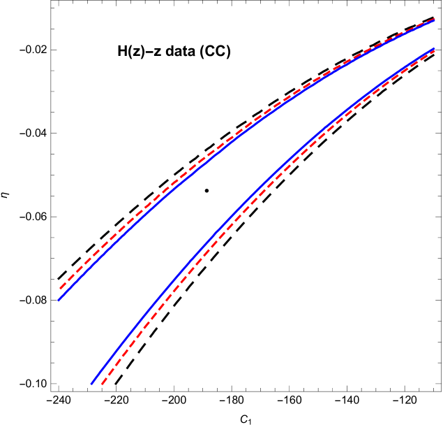
Figure 1: Confidence contours for $\eta$ vs $C_{1}$ for the CC data set.

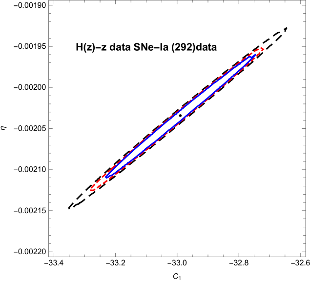
Figure 2: Confidence contours for $\eta$ vs $C_{1}$ for the 292 SNe Type-Ia data set.

Figure 2 shows the contourplot of $\eta$ against $C_{1}$ for the cosmic chronometer data set and Figure 2 shows the contours of $\eta$ vs $C_{1}$ for the 292 SNe Type-Ia data set.

3.4 Joint Analysis with CC data $+$ BAO & Supernovae Type Ia Riess 292 data + BAO

Eisenstein et al. (2005) proposed a method of joint analysis of observational data with the Baryon Acoustic Oscillation (BAO) peak parameter in order to constrain cosmological toy models. The Sloan Digital Sky Survey (SDSS) was one of the first red-shift survey by which the BAO signal was directly detected at a scale of around 100 MPc. In this survey, spectroscopic samples from around 46748 luminous red galaxies were collected which spanned over 3816 square-degrees of sky and with an approximately diameter of five billion light years. One of the major utility of this survey was that, these findings confirmed the results obtained from Wilkinson Microwave Anisotropy Probe (WMAP) using the sound horizon in the present universe. Exploring the SDSS catalog we can retrieve a such a distribution of matter existing in the universe, using which we can easily probe a BAO signal by investigating the presence of a relatively greater number of galaxies separated at the sound horizon. The methodology employed in this above mentioned analysis basically uses a blend of the angular diameter distance parameter and the Hubble parameter at that red-shift range. It is noteworthy that this analysis is self-reliant and does not depend on the measurement of the present value of Hubble parameter $H_{0}$. Moreover it does not contain any particular dark energy model and in this sense it is fairly generic in nature. Here we have examined the parameters $\eta$ and $C_{1}$ of our model from the measurements of the BAO peak for low red-shift (with range $0<z<0.35$) using standard $\chi^{2}$ analysis. The error in the measurement is given by the standard deviation in the data table, which can be fairly modelled by Gaussian distribution. It is found that the low-redshift distance measurements are quite reliant on the values of various cosmological parameters of the model like the equation of state of dark energy. Moreover such measurements do have the ability to quantify the current value of Hubble parameter $H_{0}$ directly. The BAO peak parameter may be defined by (Thakur, Ghose & Paul 2009; Paul, Thakur & Ghose 2010; Paul, Ghose & Thakur 2011; Ghose, Thakur & Paul 2012):

$${\cal A}=\frac{\sqrt{\Omega_{m}}}{E(z_{1})^{1/3}}\left(\frac{1}{z_{1}}~{}\int_{0}^{z_{1}}\frac{dz}{E(z)}\right)^{2/3}$$ (3.6)

In the above expression $E(z)=H(z)/H_{0}$ is called the normalized Hubble parameter. It is known from the SDSS survey that the red-shift $z_{1}=0.35$ is the prototypical value of red-shift which we will consider in our analysis. The integral appearing in the above expression is the dimensionless co-moving distance at the red-shift $z_{1}$. From the observational data we have motivated values for the above BAO peak ${\cal A}$. For the flat model of the universe its value is estimated to be ${\cal A}=0.469\pm 0.017$ using SDSS data (Eisenstein et al. 2005) retrieved by probing a large group of luminous red galaxies. Now the $\chi^{2}$ function for the BAO measurement can be written as

$$\chi^{2}_{BAO}=\frac{({\cal A}-0.469)^{2}}{(0.017)^{2}}$$ (3.7)

The total joint data analysis CC+BAO & SNe Type-Ia+BAO for the $\chi^{2}$ function may be defined by (Thakur, Ghose & Paul 2009; Paul, Thakur & Ghose 2010; Paul, Ghose & Thakur 2011; Ghose, Thakur & Paul 2012; Wu & Yu 2007)

$$\chi^{2}_{total}=\chi^{2}_{CC/SNe-Ia}+\chi^{2}_{BAO}$$ (3.8)

The best fit values of the model parameters $\eta$ and $C_{1}$ according to our analysis via the joint scheme of CC data and BAO peak are presented in Table 2. Finally we have drawn the contours for the predicted values of the parameters for the 66% (solid, blue), 90% (dashed, red) and 99% (dashed, black) confidence intervals and depicted them in the figures 4 and 4. Just like the previous analysis here also we see that only negative values of the parameters are allowed to realize a cosmologically feasible scenario.

Table 2: CC + BAO & SNe Type-Ia + BAO Data

$DataType$	$\eta$	$C_{1}$	$\chi^{2}_{total-min}$
CC + BAO Data	-408.965	-135.083	1874.33
SNe Type-Ia + BAO Data	-0.00209925	-36.4428	8684.41

Table2: Shows the best fit values of $\eta$, $C_{1}$ and the minimum values of the $\chi^{2}$ statistic for CC + BAO and SNe Type-Ia + BAO data.

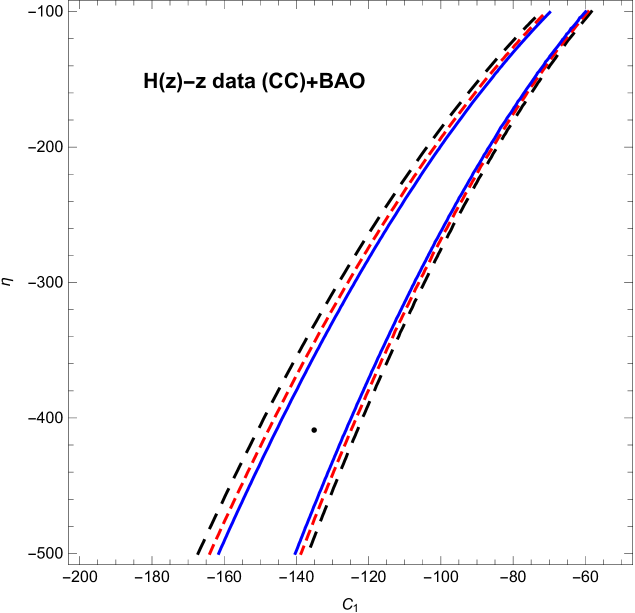
Figure 3: Confidence contours for $\eta$ vs $C_{1}$ for the CC + BAO data set.

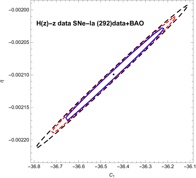
Figure 4: Confidence contours for $\eta$ vs $C_{1}$ for the 292 SNe Type-Ia + BAO data set.

Figure 4 shows the confidence contours of $\eta$ against $C_{1}$ for the CC + BAO data set and Figure 4 shows the corresponding confidence intervals of $\eta$ vs $C_{1}$ for the 292 SNe Type-Ia + BAO data set.

3.5 Joint Analysis with CC $+$ BAO $+$ CMB Data Sets & Supernovae Type Ia Riess 292 Data + BAO + CMB

Nowadays it is well known that the recent cosmic acceleration is attributed to the presence of dark energy in the universe. But although theoretically the concept seems to be relatively sound, but we are yet to get any observational evidence of the same. As a result, various investigations are underway. Of the many probes the most interesting one is via the angular scale of the first acoustic peak. Taking into account the angular scale of the sound horizon at the surface of last scattering, encoded in the Cosmic Microwave Background (CMB) power spectrum, CMB shift parameter is defined by several authors (Bond, Efstathiou & Tegmark 1997; Efstathiou & Bond 1999; Nesseris & Perivolaropoulos 2007). Although the parameter is insensitive to perturbations yet it is suitable to constrain model parameters. The first peak of the CMB power spectrum is basically a shift parameter given by

$${\cal R}=\sqrt{\Omega_{m}}\int_{0}^{z_{2}}\frac{dz}{E(z)}$$ (3.9)

where $z_{2}$ is the value of redshift corresponding to the last scattering surface. From the WMAP 7-year data available in the work of Komatsu et al. (2011) the value of the parameter has been obtained as ${\cal R}=1.726\pm 0.018$ at the redshift $z=1091.3$. Now the $\chi^{2}$ function for the CMB measurement can be written as

$$\chi^{2}_{CMB}=\frac{({\cal R}-1.726)^{2}}{(0.018)^{2}}$$ (3.10)

Now considering the three cosmological tests together, we can perform the joint data analysis for CC/SNeTypeIa+BAO+CMB. The total $\chi^{2}$ function for this case may be defined by

$$\chi^{2}_{TOTAL}=\chi^{2}_{CC/SNe-Ia}+\chi^{2}_{BAO}+\chi^{2}_{CMB}$$ (3.11)

As like before, the best fit values of the parameters $\eta$ and $C_{1}$ of our model for joint analysis of BAO and CMB with CC & with SNe Type-Ia observational data have been evaluated and the values have been presented in a tabular form in Table 3. 66% (solid, blue), 90% (dashed, red) and 99% (dashed, black) $\eta$ Vs $C_{1}$ contours are also generated for this scenario and are depicted in Figs. 6 and 6. As expected we see that the allowed range for the parameters lie in the negative region. From 6 it is evident that the predicted range for $C_{1}$ is highly constrained and tight.

Table 3: CC + BAO + CMB Data & SNe Type-Ia + BAO + CMB Data

$DataType$	$\eta$	$C_{1}$	$\chi^{2}_{TOTAL-min}$
CC +BAO+CMB Data	-408.965	-135.083	1874.33
SNe Type-Ia +BAO+CMB Data	-989730.26	-2002736.53	355032516.55

Table3: Shows the best fit values of $\eta$, $C_{1}$ and the minimum values of $\chi^{2}$ for fixed value of other parameters for CC + BAO + CMB Data and SNe Type-Ia +BAO + CMB data.

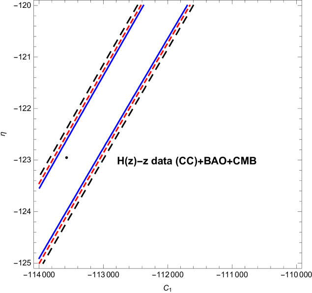
Figure 5: Confidence contours for $\eta$ vs $C_{1}$ for the CC +BAO +CMB data.

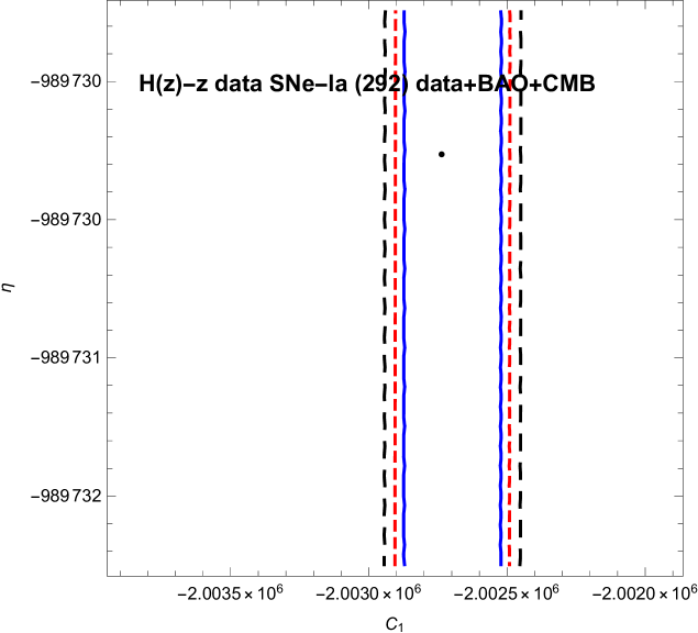
Figure 6: Confidence contours for $\eta$ vs $C_{1}$ for the 292 SNe Type-Ia +BAO +CMB data.

We obtained the plots for $q$ vs $z$ in figs.8 and 8 using the constrained values of model parameters for different data setting. We can see that the trajectories enter the negative region around $z=0.6$ which shows the late time accelerated expansion of the universe starting at $z\approx 0.6$. Here the model fits perfectly with the observations. We have also provided the plots for the $\Lambda$CDM case as reference. We see that the plots for the $\Lambda$CDM case are vertical lines which may be misleading on the first look. But actually they are not vertical lines. In a larger scale they have variations with the redshift just like the other curves. It is just because of the scale that they look like vertical lines in the comparative scenario with the plots for $w=-1/3$.

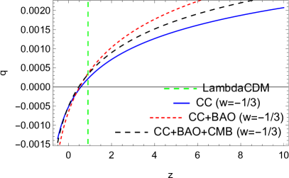
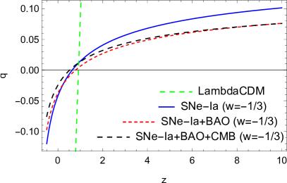
Fig.7                                                       Fig.8

Figure 7: The plot shows the deceleration parameter $q$ w.r.t. the red-shift parameter $z$ using the constrained values of parameters $\eta$ and $C_{1}$ from the CC data set.

Figure 8: The plot shows the deceleration parameter $q$ w.r.t. the red-shift parameter $z$ using the constrained values of parameters $\eta$ and $C_{1}$ from the SNe-Ia data set.

3.6 Redshift-magnitude observations from Pantheon data Sample and Supernovae Type Ia: Union2 data sample

At the turn of the last century the Supernovae Type Ia observations furnished satisfactory evidence for the fact that of late the universe has actually entered a phase of accelerated expansion. Since 1995, two teams of High redshift Supernova Search and the Supernova Cosmology Project discovered several types of Ia supernovas at the high redshifts (Perlmutter et al. 1998, 1999; Riess et al. 1998, 2004). These observations triggered the concept of dark energy as an explanation to the cosmic acceleration. Further observations by Riess et al. (2007) and Kowalaski et al. (2008) directly measured the distance modulus ($\mu(z)$) of supernovae corresponding to high redshifts. A set of $557$ data points including those from SNe-Ia known as Union2 sample is reported by Amanullah et al. (2010). From these observations the luminosity distance can be given by,

$$d_{L}(z)=(1+z)H_{0}\int_{0}^{z}\frac{dz^{\prime}}{H(z^{\prime})}$$ (3.12)

where $z^{\prime}$ is the independent variable in the above integral. Moreover the distance modulus (which is defined as the difference between the apparent magnitude and the absolute magnitude of any astronomical object) is given by,

$$\mu(z)=5\log_{10}\left[\frac{d_{L}(z)/H_{0}}{1MPc}\right]+25$$ (3.13)

In the figs. 10, 10 and 11 we have obtained the best fit of the distance modulus for our theoretical EMSG model for the constrained values of parameters both from CC and SNe-Ia observations. These have been compared with the union2 data sample represented by the blue dots. In fig.10 we have used the pure CC and SNe-Ia data to obtain the best fit. We can see that the best fits show significant deviation from the union2 data sample, with CC data showing a greater deviation. In 10 the results obtained from the joint analysis of CC+BAO and SNe-Ia+BAO have been used to obtain the best fits. Here we see that the deviations from the union2 data sample have considerably reduced and the fit obtained from the CC+BAO is in agreement with the union2 sample around $z=1$. But the fit from SNe-Ia+BAO data still has large deviations from the union2 sample. In 11 fits are obtained from the joint analysis of CC+BAO+CMB and SNe-Ia+BAO+CMB. Just like 10 here also we witness a significant agreement of CC+BAO+CMB fit with the union2 sample data. But the fit from SNe-Ia+BAO+CMB is still significantly deviated from the sample data. This analysis throws light on the two data sets in a comparative scenario. In a comparative scenario with union2 sample both CC data and SNe-Ia data show significant deviations, but when joint analysis with BAO and CMB is considered, CC data shows agreement with the union2 sample at around $z=1$.

In figs.12 and 13 we have plotted the distance modulus of our model for different values of the parameters $\eta$ and $C_{1}$, with the recently published Pantheon data points in the background represented by the blue cluster. In the fig.12 we have varied $\eta$ keeping $C_{1}$ constant and in fig.13 we have varied $C_{1}$ keeping $\eta$ constant. In both the figures the Pantheon cluster with error bars actually helps us to get a comparative outlook of our theory with the recent astronomical observations. We can get a feel of the degree of compliance of our model with the recent observations.

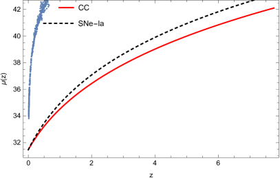
Fig.9                                                               Fig.10       

Figure 9: The plot shows the distance modulus $\mu(z)$ w.r.t. the red-shift parameter $z$ using the constrained values of parameters $\eta$ and $C_{1}$ from the CC and SNe-Ia data sets. The blue dots show the Union2 sample points.

Figure 10: The plot shows the distance modulus $\mu(z)$ w.r.t. the red-shift parameter $z$ using the constrained values of parameters $\eta$ and $C_{1}$ from the CC+BAO and SNe-Ia+BAO data sets. The blue dots show the Union2 sample points.

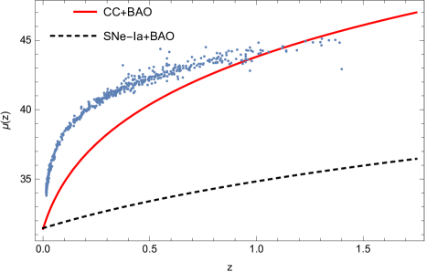
Figure 11: The plot shows the distance modulus $\mu(z)$ w.r.t. the red-shift parameter $z$ using the constrained values of parameters $\eta$ and $C_{1}$ from the CC+BAO+CMB and SNe-Ia+BAO+CMB data sets. The blue dots show the Union2 sample points.

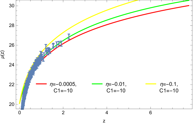
Figure 12: The plot shows the distance modulus $\mu(z)$ w.r.t. the red-shift parameter $z$ for different values of parameters $\eta$ keeping $C_{1}$ constant. The blue dots show the Pantheon sample points.

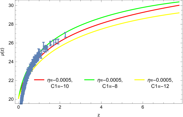
Figure 13: The plot shows the distance modulus $\mu(z)$ w.r.t. the red-shift parameter $z$ using different values of parameters $C_{1}$ keeping $\eta$ constant. The blue dots show the Pantheon sample points.

4 Multi-component Universe model

In the previous section we have considered a mono-component universe model where the matter sector of the universe was considered to be composed of a single component, given by a cosmological fluid with EoS $w=-1/3$. But the observations favour a multi-component matter universe. So in this section we will consider dust in our model along with the cosmological fluid content. It is well-known that the dust component of matter is pressure-less and constitutes about $30\%$ of the universe. Most of this portion is invisible in nature because it does not interact with the electromagnetic field. Moreover this portion of matter has minimum interaction with the baryonic component of the universe and interacts only through gravitational interaction. Here we consider the energy density of matter as $\rho=\rho_{fluid}+\rho_{dust}$, where $\rho_{dust}$ and $\rho_{fluid}$ represent the energy densities of dust and other fluid component respectively. Moreover the total matter pressure will remain the same $p=p_{fluid}$ because dust is pressureless, i.e., $p_{dust}=0$. This will eventually make the equation state of dust as $w_{dust}=p_{dust}/\rho_{dust}=0$. For this two-component model we get $T_{\mu\nu(i)}T^{\mu\nu(i)}=\rho_{i}^{2}\left(1+3w_{i}^{2}\right)$, where $i$ represents the fluid component. So for dust we have $T_{\mu\nu(i)}T^{\mu\nu(i)}=\rho_{dust}^{2}$ and for the other fluid component $T_{\mu\nu(i)}T^{\mu\nu(i)}=\rho_{fluid}^{2}\left(1+3w_{fluid}^{2}\right)$. The modified FLRW equations for this model take the forms,

$$-3f_{R}\Big{(}\dot{H}+H^{2}\Big{)}+\frac{f}{2}+3H\dot{f_{R}} = \kappa^{2}\Big{(}\rho_{fluid}+\rho_{dust}+\frac{1}{\kappa^{2}}f_{\mathbf{T^{2}}}\Theta^{2}\Big{)}\,,$$ (4.1)

$$-f_{R}(\dot{H}+3H^{2})+\frac{1}{2}f+\ddot{f_{R}}+2H\dot{f_{R}} = -\kappa^{2}p_{fluid}\,,$$ (4.2)

where

$$\mathbf{\Theta^{2}}:=\Theta_{\mu\nu}\Theta^{\mu\nu}=\left(\rho_{fluid}+\rho_{dust}\right)^{2}+4p\left(\rho_{fluid}+\rho_{dust}\right)+3p_{fluid}^{2}$$ (4.3)

Now the individual continuity equations for the different matter components are given below:

For cosmological fluid:

$$\dot{\rho}_{fluid}+3H(w_{fluid}+1)\rho_{fluid} = -f_{\mathbf{T^{2}}}\left[3\left(3w_{fluid}^{2}+4w_{fluid}+1\right)H\rho_{fluid}^{2}+\left(3w_{fluid}^{2}+8w_{fluid}+1\right)\rho_{fluid}\dot{\rho}_{fluid}\right]$$ (4.4)

$$-\left(3w_{fluid}^{2}+4w_{fluid}+1\right)\rho_{fluid}^{2}\dot{f}_{\mathbf{T^{2}}}\,.$$

For Dust:

$$\dot{\rho}_{dust}+3H\rho_{dust}=-f_{\mathbf{T^{2}}}\left(3H\rho_{dust}^{2}+\rho_{dust}\dot{\rho}_{dust}\right)-\rho_{dust}^{2}\dot{f}_{\mathbf{T^{2}}}$$ (4.5)

Now the solution of the continuity equation for the fluid will be similar to the one obtained in the previous section for the single component fluid model. For the continuity equation of dust we see that, it is difficult to get a solution in a model independent way. So we proceed to get a solution for the model $f(R,\mathbf{T^{2}})=R+\eta\mathbf{T^{2}}$. Solving the continuity equation of dust for this model we get,

$$\rho_{dust}=C_{2}\left(1+z\right)^{3}$$ (4.6)

where $C_{2}$ is the constant of integration. Now we can compare the density components by studying their evolution with time. To do this we consider the first FLRW equation as,

$$3H^{2}=\kappa^{2}\left(\rho_{dust}+\rho_{fluid}+\rho_{modified}\right)$$ (4.7)

from the above equation we see that $\Omega_{dust}+\Omega_{fluid}+\Omega_{modified}=1$, where $\Omega_{dust}=\frac{\kappa^{2}\rho_{dust}}{3H^{2}}$, $\Omega_{fluid}=\frac{\kappa^{2}\rho_{fluid}}{3H^{2}}$ and $\Omega_{modified}=\frac{\kappa^{2}\rho_{modified}}{3H^{2}}$. These are the dimensionless density components of the universe for our model. We will study the evolution characteristics of these density components.

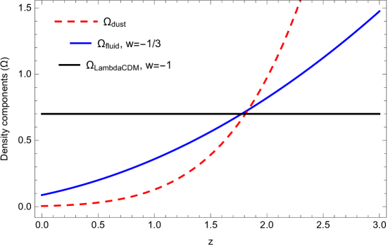
Figure 14: The plot shows the evolution of density components $\Omega$ w.r.t. the red-shift parameter $z$. Plot for the $\Lambda$CDM case have been provided as reference. The initial conditions are taken as $C_{1}=-135$, $\eta=-408$, $C_{2}=0.004$ and $\kappa=1$.

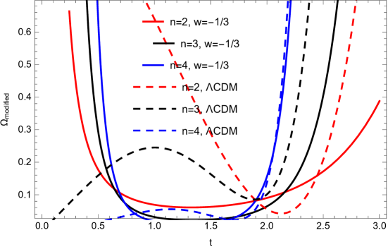
Figure 15: The plot shows the evolution of the density component of modified gravity $\Omega_{modified}$ w.r.t. time $t$ for different values of parameters $n$. The corresponding scenarios for the $\Lambda$CDM model have also been presented as reference. The model parameters are taken as $C_{1}=-135$, $\eta=-408$, $C_{2}=0.2$, $w=-1/3$, $z_{0}=0.1$ and $\kappa=1$.

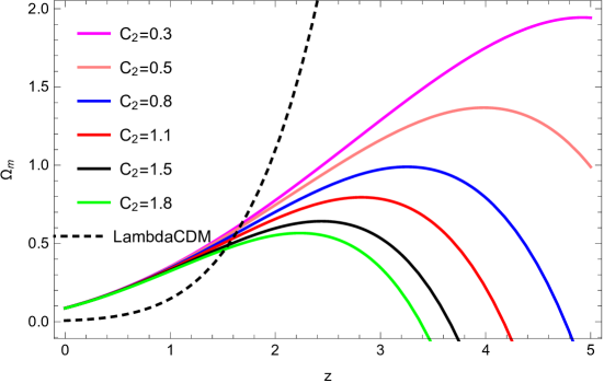
Figure 16: The plot shows the evolution of the total matter density component i.e. $\Omega_{m}=\Omega_{dust}+\Omega_{fluid}$ w.r.t. redshift $z$ for different values of parameters $C_{2}$ for $w=-1/3$. The case for $\Lambda$CDM have also been presented. The model parameters are taken as $C_{1}=-135$, $\eta=-408$, $w=-1/3$.

In fig.14 we have plotted the evolution of the density components of dust and matter fluid with $w=-1/3$ against the redshift parameter $z$. Here we have considered the constrained values of the parameters for the fluid. This helps us to compare the evolution of a single component fluid model with dust. Here the $C_{2}$ parameter is free and so by suitably fine tuning the parameter we can get our model to follow the observations and thus get an idea about correct the parametric value. It should be stated here that both the matter components are non-exotic in nature. In fig.15 we have studied the behaviour of the density component arising from the modification of gravity against time. Since our matter content (dust and fluid) is non-exotic in nature, the effects coming from the EMSG modifications to gravity should be responsible for the accelerated expansion of the universe. Here we have used the redshift-time dependence as $z(t)=z_{0}t^{n}$, where $z_{0}$ and $n$ are constants. We have studied the evolution of $\Omega_{modified}$ against time $t$ for different values of the power $n$. It is seen that in the early times there is a significant effect of the modification of gravity. The density component due to EMSG modification peaks in the early universe and wanes out with the evolution of time. This is in complete correspondence with the work of Akarsu et. al 2018. Probably this peak is responsible for the cosmological inflation in the early universe. With the evolution of time $\Omega_{modified}$ decays and universe is dominated by matter in the intermediate phase. Finally again $\Omega_{modified}$ shoots up and dominates the universe in late times, thus accounting for the recent cosmic acceleration. It should be mentioned over here that the contributions from the modified gravity are actually equivalent to the exotic contributions from a dark energy model. So our non-exotic matter along with the EMSG modifications gives quite a reasonable proposition. In fact it is almost meaningless to consider both exotic matter and contributions from modified gravity because in such a scenario it is quite obvious that an accelerated expansion will always be realized irrespective of initial conditions. So our multi-component model is in complete agreement with the evolution history of the universe. The overall evolution of the system will be the combination of the contributions from the three component: fluid, dust and modified gravity.

In figure 16 we have plotted the total matter density components, i.e., $\Omega_{m}=\Omega_{dust}+\Omega_{fluid}$ against the redshift $z$. Here the equation of state of the fluid is taken as $w=-1/3$ corresponding to the solution that we have got. So it is obvious that both the components of $\Omega_{m}$ are relatively non-exotic in nature. The acceleration is driven by the pure geometric effects of modified gravity. From the observations we know that the total share of $\Omega_{m}$ should be around 0.3. In our study we see that the matter density decreases as the universe evolves, which is obvious for an expanding universe. In fig.16 we have obtained plots for different values of the dust parameter $C_{2}$. We see that in almost all the cases we can realize a scenario when $\Omega_{m}\approx 0.3$ corresponding to some value of redshift. From the figure we can see that irrespective of the value of $C_{2}$ this is happening for $z\approx 1$. Note that we have used the constrained values of $\eta$ and $C_{1}$ that we have obtained from our observational data analysis. Obviously by changing these parameters we can alter the redshift value at which we realize $\Omega_{m}\approx 0.3$, but since we have used the constrained values to obtain the plot, it is reasonable to be satisfied with $z\approx 1$. This argument actually helps us to address the degeneracy problem with the value of $\Omega_{m}$ mentioned in the work Faria et. al 2019. From the observations of galaxy rotation curves and gravitational lensing it is also seen that most of this matter is dark in nature. In all the plots 14, 15 and 16, we have presented the scenario for the $\Lambda$CDM model as a reference for the other trajectories. In the figs.18 and 18, we have plotted the deceleration parameter $q$ against the redshift parameter $z$ for our multi-component model. We see that for the both the datasets we get late time accelerated expansion of the universe, but it seems that the model fits better with the CC data. This is because the origin of the accelerating phase is more pushed towards the redshift value $z\approx 0.6$ for the CC data (fig.18) as compared to the SNe data (fig.18). From this, we can contemplate that the constrained values of the model parameters of the EMSG model gives more realistic results with the CC data. We have also presented the trajectory for the $\Lambda$CDM case for comparison.

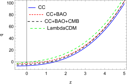
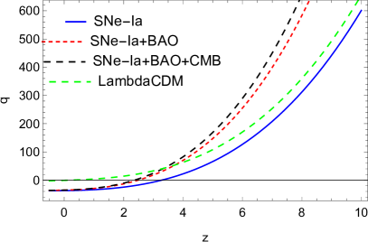
Fig.17                                                       Fig.18

Figure 17: The plot shows the deceleration parameter $q$ w.r.t. the red-shift parameter $z$ using the constrained values of parameters $\eta$ and $C_{1}$ from the CC data set for the multi-component model.

Figure 18: The plot shows the deceleration parameter $q$ w.r.t. the red-shift parameter $z$ using the constrained values of parameters $\eta$ and $C_{1}$ from the SNe-Ia data set for the multi-component model.

5 Discussion and Conclusion

In this work we have studied the increasingly popular $f(R,T^{2})$ theory. The theory has been constrained using observational data. Two different data-sets have been used for this purpose, namely the cosmic chronometer (CC) data and the Supernovae (SNe) Type-Ia data (See Appendix for the full data table of CC data). It should be mentioned that both these data are a set of $z-H(z)$ points, which is the prime requirement of our data analysis mechanism. The energy momentum squared gravity has a basic mathematical issue regarding the integration of the continuity equation. The equation cannot be integrated generically using the known mathematical methods. In fact it was shown in Board & Barrow (2017) that it can be integrated for only two values of the barotropic parameter viz. $w=-1$ and $w=-1/3$. Here we have integrated the continuity equation for both these values and used the expression for energy density obtained for $w=-1/3$ in the further computations. The cosmological implications of our obtained solution is discussed in detail and all possible limits of the solution is considered including its reconciliation to GR as $\eta\rightarrow 0$.

The Hubble parameter $H$ is expressed in terms of the redshift parameter $z$ in order to suit the nature of observational data used. Then we have used this in the set-up to minimize the $\chi^{2}$ distribution. In the $\chi^{2}$ variable we have actually compared the theoretically obtained expression for the Hubble parameter $H$ in terms of $z$ with the observed values of $H$ corresponding to $z$ from the data. The best fit values of the model parameters are then obtained from the $\chi^{2}$ function. We see that the model has two free parameters $\eta$ and $C_{1}$. Fitting the model with the data we have constrained these two parameters and found out the most likely values of them. Further we have used the peak parameters from BAO and CMB observations and clubbed them with the two data-sets to further constrain the parameters. For each data-set analysis have been done in three steps. For the CC data, we have performed analysis with pure 30 points CC data, CC+BAO and CC+BAO+CMB. Similarly for SNe-Ia data analysis have been performed with the 292 point SNe-Ia data, SNe-Ia+BAO and SNe-Ia+BAO+CMB. The joint analysis is expected to give far better results as far as the evolution of the universe is concerned. For each set we have obtained the constrained values of the free parameters $\eta$ and $C_{1}$. We have seen that both the parameters acquire values in the negative range which is completely consistent with a satisfactory cosmological behaviour. We have also recorded the minimum value of the $\chi^{2}$ statistic, which is the basic statistical tool used in all the analysis. For each analysis we have presented confidence contours for the predicted values of the free parameters showing the $66\%$, $90\%$ and $99\%$ confidence levels. From the confidence contours we get clear idea about the values of the model parameters along with their error bounds. The black dots in each contour plots represent the best possible value of the parameters as predicted by our statistical set-up correlating the observational data and the theoretical model. Finally a best fit of distance modulus is obtained for the theoretical EMSG model both for CC and SNe-Ia data sets. It was seen that they show significant deviations with the union2 sample data. However the deviation for the CC+BAO and CC+BAO+CMB joint analysis is considerably reduced and agreement with union2 sample is established around $z=1$. Moreover we have also obtained a best fit distance modulus of our model against the recently published Pantheon data sample and tried to get an idea about the compliance of the theoretical model with recent observations.

Finally we have studied a multi-component universe by adding dust to our fluid model. Fluid with equation of state $w=-1/3$ is taken with dust with equation of state $w=0$ to constitute the non-exotic matter part of the universe. The acceleration in such a model is supposed to be driven by the EMSG modifications to the gravity characterized by the density component arising from the modified gravity. We have studied the evolution of all the three density components $\Omega_{dust}$, $\Omega_{fluid}$ and $\Omega_{modified}$ in comparative scenarios. We have seen that for suitable initial conditions our model gives the values which are favoured by observations. We have also investigated the trends of the deceleration parameter for the multi-component scenario. All the results have been compared with those of the standard $\Lambda$CDM model. To sum up, the present analysis discusses the correlation of the theoretical EMSG model with observational data and clearly is a significant development of the energy momentum squared gravity model as well as our understanding of the universe.

6 Appendix

See Table 4 for the $30$ point Cosmic Chronometer Data.

Table 4: Cosmic Chronometer $30$ point Data Set

$z$	$H(z)$	$\sigma(z)$	$z$	$H(z)$	$\sigma(z)$
0.07	69	$\pm$ 19.6	0.4783	80.9	$\pm$ 9
0.09	69	$\pm$ 12	0.48	97	$\pm$ 62
0.12	68.6	$\pm$ 26.2	0.593	104	$\pm$ 13
0.17	83	$\pm$ 8	0.68	92	$\pm$ 8
0.179	75	$\pm$ 4	0.781	105	$\pm$ 12
0.199	75	$\pm$ 5	0.875	125	$\pm$ 17
0.2	72.9	$\pm$ 29.6	0.88	90	$\pm$ 40
0.27	77	$\pm$ 14	0.9	117	$\pm$ 23
0.28	88.8	$\pm$ 36.6	1.037	154	$\pm$ 20
0.352	83	$\pm$ 14	1.3	168	$\pm$ 17
0.3802	83	$\pm$ 13.5	1.363	160	$\pm$ 33.6
0.4	95	$\pm$ 17	1.43	177	$\pm$ 18
0.4004	77	$\pm$ 10.2	1.53	140	$\pm$ 14
0.4247	87.1	$\pm$ 11.2	1.75	202	$\pm$ 40
0.44497	92.8	$\pm$ 12.9	1.965	186.5	$\pm$ 50.4

Table 4: Shows the 30 point cosmic chronometer $z-H(z)$ data with the standard error $\sigma(z)$.

References

-
[1]
Akarsu O., Barrow J. D., Cikintoglu S., Eksi K. Y., Katirci N., 2018, Phys. Rev. D, 97, 12
Akarsu O., Katirci N., Kumar S., Nunes R. C., Sami M., 2018, Phys. Rev. D, 98, 6
Akarsu O, Katirci N., Kumar S., 2018, Phys. Rev. D, 97, 2
Akarsu O., Barrow, J. D., Board C. V. R., Uzun N. M., Vazquez J. A., 2019, Eur. Phys. J. C, 79, 846
Amanullah R. et al., 2010, Astrophys. J., 716, 712
Amendola L., Polarski D., Tsujikawa S., 2007, Phys. Rev. Lett., 98, 131302
Amendola L., Gannouji R,. Polarski D., Tsujikawa S., 2007, Phys. Rev. D, 75, 083504
Astier P. et al., 2006, Astron. Astrophys., 447, 31
Azizi T., Yaraie E., 2014, Int. J. Mod. Phys. D., 23, 1450021
Bahamonde S., Marciu M., Rudra P., 2019, Phys. Rev. D, 100, 8
Bertolami O., Boehmer C. G., Harko T., Lobo F. S. N., 2007, Phys. Rev. D, 75, 104016
Board C. V. R., Barrow J. D., 2017, Phys. Rev. D, 96, 12
Bond J. R., Efstathiou G., Tegmark M., 1997, Mon. Not. R. Astron. Soc., 291, L33
Brax P., 2018, Rep. Prog. Phys., 81, 1
Capozziello S., De Laurentis M., Faraoni V., 2010, Open Astron. J., 3, 49
Carroll S. M., Duvvuri V., Trodden M., Turner M. S., 2004, Phys. Rev. D, 70, 043528
Clifton T., Ferreira P. G., Padilla A., Skordis C., 2012, Phys. Rept., 513, 1
Cognola G., Elizalde E., Nojiri S., Odintsov S. D., Sebastiani L., Zerbini S., 2008, Phys. Rev. D, 77, 046009
De Felice A., Tsujikawa S., 2010, Living Rev. Relativ., 13, 3
Efstathiou G., Bond J. R., 1999, Mon. Not. R. Astron. Soc., 304, 75
Eisenstein D. J. et al., 2005, Astrophys. J., 633, 560
Faria M. C. F., Martins C. J. A. P, Chiti, F., Silva B. S. A., 2019, Astron. Astrophys., 625, A127
Farooq O., Ratra B., 2013, Astrophys. J., 766, L7
Ghose S., Thakur P., Paul B. C., 2012, Mon. Not. R. Astron. Soc., 421, 20
Gomez-Valent A., Amendola L., 2019, presentation at ”15th Marcel Grossmann Meeting on Recent Developments in Theoretical and Experimental General Relativity, Astrophysics and relativistic Field Theories (MG15)” Rome, Italy, July 1-7, 2018
Haghani Z., Harko T., Lobo F. S. N., Sepangi H. R., Shahidi S., 2013, Phys. Rev. D, 88, 4
Harko T., 2008, Phys. Lett. B., 669, 376
Harko T., 2010, Phys. Rev. D, 81, 044021
Harko T., Lobo F. S. N., 2010, Eur. Phys. J. C, 70, 373
Harko T., Lobo F. S. N., Nojiri S., Odintsov S. D., 2011, Phys. Rev. D, 84, 024020
Jimenez R., Loeb A., 2002, Astrophys. J., 573, 37
Katirci N., Kavuk M., 2014, Eur. Phys. J. Plus, 129, 163
Keskin A., 2018, AIP Conf. Proc., 2042, 1
Komatsu E. et al., 2011, Astrophys. J. Suppl., 192, 18
Kowalaski M. et al., 2008, Astrophys. J., 686, 749
Martin J., 2012, C R Phys, 13, 566
Moraes P. H. R. S., Sahoo P. K., 2018, Phys. Rev. D, 97, 2
Moresco M., 2015, Mon. Not. R. Astron. Soc., 450, 1
Moresco M. et al., 2016, J. Cosmol. Astropart. Phys., 1605, 014
Nagpal R., Singh J. K., Beesham A., Shabani H, 2019, Ann. Phys., 405, 234
Nari N., Roshan M., 2018, Phys. Rev. D, 98, 2
Nojiri S., Odintsov S. D., 2006, Phys. Rev. D, 74, 086005
Nojiri S., Odintsov S. D., 2007, Int. J. Geom. Meth. Mod. Phys., 4, 115
Nojiri S., Odintsov S. D., Oikonomou V. K., 2017, Phys. Rept., 692, 1
Nesseris S., Perivolaropoulos L., 2007, J. Cosmol. Astropart. Phys., 0701, 018
Paliathanasis A., Tsamparlis M., Basilakos S., 2011, Phys. Rev. D, 84, 123514
Paliathanasis A., 2016, Class. Quantum Grav., 33, 7
Paul B. C., Thakur P., Ghose S., 2010, Mon. Not. R. Astron. Soc., 407, 415
Paul B. C., Ghose S., Thakur P., 2011, Mon. Not. R. Astron. Soc., 413, 686
Perlmutter S. et al. 1998, Nature, 391, 51
Perlmutter S. et al., 1999, Astrophys. J., 517, 565
Riess A. G. et al., 1998, Astron. J., 116, 1009
Riess A. J. et al., 2004, Astrophys. J., 607, 665
Riess A. J. et al., 2007, Astrophys. J., 659, 98
Roshan M., Shojai F., 2016, Phys. Rev. D, 94, 4
Simon J., Verde L., Jimenez R., 2005, Phys. Rev. D, 71, 123001
Song Y-S., Hu W., Sawicki I., 2007, Phys. Rev. D, 75, 044004
Sotiriou T. P., Faraoni V., 2010, Rev. Mod. Phys., 82, 451
Spergel D. N. et al., 2003, Astrophys. J. Suppl., 148, 175
Stern D., Jimenez R., Verde L., Kamionkowski M., Stanford S., 2010, J. Cosmol. Astropart. Phys., 02, 008
Thakur P., Ghose S., Paul B. C., 2009, Mon. Not. R. Astron. Soc., 397, 1935
Wu P., Yu H. W., 2007, Phys. Lett. B, 644, 16
Zhang C., Zhang H., Yuan S., Zhang T.-J., Sun Y.-C., 2014, Res. Astron. Astrophys., 14, 10
Zlatev I, Wang L.-M. Steinhardt P. J, 1999, Phys. Rev. Lett., 82, 896