Negative heat capacity for hot nuclei using formulation
from the microcanonical ensemble
INDRA Collaboration

Abstract

By using freeze-out properties of multifragmenting hot nuclei produced in quasifusion central ¹²⁹Xe+^natSn collisions at different beam energies (32, 39, 45 and 50 AMeV) which were estimated by means of a simulation based on experimental data collected by the $4\pi$ INDRA multidetector, heat capacity in the thermal excitation energy range 4 - 12.5 AMeV was calculated from total kinetic energies and multiplicities at freeze-out. The microcanonical formulation was employed. Negative heat capacity which signs a first order phase transition for finite systems is observed and confirms previous results using a different method.

An important challenge of heavy-ion collisions at intermediate energies is the identification and characterization of the nuclear liquid-gas phase transition in hot nuclei, which has been theoretically predicted for nuclear matter Sch82 ; Cur83 ; Jaq83 ; Mul95 ; Wel14 . At present one can say that huge progress has been made even if some points can be deeper investigated WCI06 ; Bor08 ; Bor19 ; Wad19 ; Lin19 . Statistical mechanics for finite systems appeared as a key issue to progress, revealing specific first-order phase transition signatures related to the consequences of the local convexity of the entropy Lab90 ; Wal94 ; Gro97 ; Gulm02 ; Cho04 ; Tou09 ; Cam09 . By considering the microcanonical ensemble with energy as extensive variable, the convex intruder implies a backbending in the temperature (first derivative of entropy) at constant pressure Cho00 and correlatively a negative branch for the heat capacity (second derivative of entropy). Experimentally, these two converging signatures have been observed in hot nuclei from different analyses I79-Bor13 ; MDA00 ; NicPHD ; I46-Bor02 ; I63-NLN07 of homogeneous event samples. It is important to recall here that signals of phase transition in hot nuclei are only meaningful at the level of statistical ensembles constructed from the outcome of carefully selected collisions Bor19 . Another consequence of the entropy curvature anomaly manifests itself when systems are treated in the canonical ensemble. In this case a direct phase transition signature is the presence of a bimodal distribution of an order parameter Cho01 such as the charge (size) of the largest fragment (Z_max) of multifragmentation partitions I72-Bon09 . As far as microcanonical heat capacity calculation is concerned, a question still subsists. It concerns one hypothesis made in the method used up to now: the same temperature was associated with both internal excitation and thermal motion of emitted fragments, which is not physically obvious if one remembers that the level density is expected to vanish at high excitation energies Tub79 ; Dean85 ; Koo87 ; Sou15 . Moreover it was shown in simulations compared to data that widths of the fragment velocity spectra cannot be reproduced with the hypothesis of a common temperature for intrinsic and kinetic degrees of freedom I66-Pia08 .

In the present letter we will give heat capacity information for experimental data from microcanonical formulae and by ignoring the hypothesis of a single temperature, which requires the introduction of a limiting temperature for fragments.

We first briefly recall the method proposed for measuring heat capacity using partial energy fluctuations with a microcanonical sampling Cho99 ; Gul00 ; Cho00 . The prescription is based on the fact that, for a given total energy, the average partial energy stored in a part of the system is a good microcanonical thermometer, while the associated fluctuations can be used to construct the heat capacity. From experiments the most simple decomposition of the thermal excitation energy is in a kinetic part, $E_{k}$, and a potential part, $E_{pot}$ (Coulomb energy + total mass excess). These quantities have to be determined at freeze-out and consequently it is necessary to trace back this configuration on an event by event basis. The true configuration needs the knowledge of the freeze-out volume and of all the particles evaporated from primary hot fragments including the (undetected) neutrons. Consequently some working hypotheses are used, constrained by specific experimental results (see for example MDA02 ). Then, the experimental correlation between the kinetic energy per nucleon $E_{k}$/$A$ and the thermal excitation energy per nucleon $E^{*}$/$A$ of the considered system can be obtained event by event as well as the variance of the kinetic energy $\sigma_{k}^{2}$. Note that $E_{k}$ is calculated by subtracting the potential part $E_{pot}$ from the thermal excitation energy $E^{*}$ and consequently kinetic energy fluctuations at freeze-out reflect the configurational energy fluctuations. In the microcanonical ensemble with total energy $E^{*}$ the total degeneracy factor is simply given by the folding product of the individual degeneracy factors $W_{k}=exp(S_{k}(E_{k}))$ and $W_{pot}=exp(S_{pot}(E_{pot}))$ where $S_{k}$($S_{pot}$) is the entropy of the kinetic (potential) part. One can then define for the total system as well as for the two subsystems the microcanonical temperatures and the associated heat capacities $C_{k}$ and $C_{pot}$. If we consider now the kinetic energy distribution when the total energy is $E^{*}$ we get

$$\noindent P_{E^{*}}(E_{k})=exp(S_{k}(E_{k})+S_{pot}(E^{*}-E_{k})).$$ (1)

Then the most probable kinetic energy $\overline{E_{k}}$ is defined by the equality of the partial microcanonical temperatures $T_{k}(\overline{E_{k}})$ = $T_{pot}(E^{*}-\overline{E_{k}})$ and $\overline{E_{k}}$ can be used as the microcanonical thermometer. An estimator of the microcanonical temperature of the system can be obtained by inverting the kinetic equation of state:

$$\noindent<E_{k}>=\langle\sum_{i=1}^{M}a_{i}\rangle T^{2}+\langle\frac{3}{2}(M-1)\rangle T$$ (2)

The brackets $\langle\rangle$ indicate the average on events with the same $E^{*}$, $a_{i}$ is the level density parameter and M the multiplicity at freeze-out. In this expression the same temperature is associated with both internal excitation and thermal motion of fragments. An estimate of the total microcanonical heat capacity is extracted using three equations.

$$\noindent C_{k}=\frac{\delta<E_{k}/A>}{\delta T},$$ (3)

is obtained by taking the derivative of $<E_{k}/A>$ with respect to $T$.

Using a Gaussian approximation for $P_{E^{*}}(E_{k})$ the kinetic energy variance can be calculated as

$$A\sigma_{k}^{2}\simeq T^{2}\frac{C_{k}C_{pot}}{C_{k}+C_{pot}};$$ (4)

Eq. (4) can be inverted to extract, from the observed fluctuations, an estimate of the microcanonical heat capacity:

$$\noindent(\frac{C}{A})_{micro}\simeq C_{k}+C_{pot}\simeq\frac{C_{k}^{2}}{C_{k}-\frac{A\sigma_{k}^{2}}{T^{2}}}.$$ (5)

From Eq. (5) we see that the specific microcanonical heat capacity $(C/A)_{micro}$ becomes negative if the normalized kinetic energy fluctuations $A\sigma_{k}^{2}/T^{2}$ overcome $C_{k}$. It is interesting to note that the constraint of energy conservation leads in the phase transition region to larger fluctuations than in the canonical case where the total energy is free to fluctuate. This is because the kinetic energy part is forced to share the total available energy with the potential part: when the potential part presents a negative heat capacity the jump from “liquid” to “gas” induces strong fluctuations in the energy partitioning.

Direct formulae have been proposed in Ref. Radut02 to calculate heat capacity but never used to extract information from data. They are derived within the microcanonical ensemble by considering fragments interacting only by Coulomb and excluded volume, which corresponds to the freeze-out configuration. Within this ensemble, the statistical weight of a configuration $c$, defined by the mass, charge and internal excitation energy of each of the constituting $M_{c}$ fragments, can be written Radut02 ; I79-Bor13 as

$$W_{c}(A,Z,E^{*},V)=\frac{1}{M_{c}!}\chi V^{M_{c}}\prod_{n=1}^{M_{c}}\left(\frac{\rho_{n}(\epsilon_{n})}{h^{3}}(mA_{n})^{3/2}\right)$$

$$\times~{}\frac{2\pi}{\Gamma(3/2(M_{c}-d))}~{}\frac{1}{\sqrt{({\rm det}I})}~{}\frac{(2\pi K)^{(3/2)(M_{c}-d)-1}}{(mA)^{3/2}},$$ (6)

where $A$, $Z$, $E^{*}$ and $V$ are respectively the mass number, the atomic number, the thermal excitation energy and the freeze-out volume of the system. $E^{*}$ is used up in fragment formation, fragment internal excitation, fragment-fragment Coulomb interaction and thermal kinetic energy $K$. $I$ is the inertial tensor of the system whereas $\chi V^{M_{c}}$ stands for the free volume or, equivalently, accounts for inter-fragment interaction in the hard-core idealization. $\rho_{n}(\epsilon_{n})$ represents the fragment level density (see  Radut00 for the complete expression). $d$ takes respectively values 0, 1 and 2 for energy, energy plus linear momentum and energy plus linear and angular momenta conservations. In the following $d$ will be fixed to 1 to ensure coherence with simulations which are used. Taking into account that $S=\ln Z=\ln\sum_{c}W_{c}$, the microcanonical temperature is deduced from its statistical definition Radut02 :

$$T=\left(\frac{\partial S}{\partial E^{*}}\right)^{-1} = \left(\frac{1}{\sum_{c}W_{c}}\sum_{c}W_{c}(3/2M_{c}-5/2)/K\right)^{-1}$$ (7)

$$= \langle(3/2M_{c}-5/2)/K\rangle^{-1}.$$ (8)

The notation $\langle\rangle$ refers to the average over the ensemble states. The heat capacity of the system, $C$, is related to the second derivative of the entropy by the equation $\partial^{2}S/\partial E^{*2}$ = $-1/CT^{2}$. Thus, one can evaluate the second derivative of the system entropy versus $E$ (Eq. (9)) or alternatively the heat capacity $C$ (Eq. (10))

$$\frac{\partial^{2}S}{\partial E^{*2}} = \langle\frac{(3/2M_{c}-5/2)(3/2M_{c}-7/2)}{K^{2}}\rangle$$ (9)

$$- \langle\frac{(3/2M_{c}-5/2)}{K}\rangle^{2}$$

$$C=\left(1-T^{2}\langle\frac{(3/2M_{c}-5/2)(3/2M_{c}-7/2)}{K^{2}}\rangle\right)^{-1}$$ (10)

These two quantities only depend on two parameters $M_{c}$ and $K$ which must be estimated at freeze-out.

In Refs. I58-Pia05 ; I66-Pia08 we presented simulations which correctly reproduce most experimental observables and estimate freeze-out properties in a fully consistent way. They concern hot nuclei which undergo multifragmentation
formed in central collisions and selected by event shape sorting (quasifused systems, QF, from ${}^{129}Xe$+${}^{nat}Sn$, 32-50 AMeV) I69-Bon08 . We will use the event by event properties at freeze-out which were inferred to calculate the required quantities $M_{c}$ and $K$.

Experimental data were collected with the 4$\pi$ multidetector INDRA described in detail in Ref. I3-Pou95 ; I5-Pou96 . Accurate particle and fragment identifications were achieved and the energy of the detected products was measured with an accuracy of 4%. Further details can be found in Ref.I14-Tab99 ; I33-Par02 ; I34-Par02 .

The method for reconstructing freeze-out properties from simulations I58-Pia05 ; I66-Pia08 requires data with a very high degree of completeness, (measured fraction of the available charge $\geq$93% of the total charge of the system), crucial for a good estimate of Coulomb energy. QF sources are reconstructed, event by event, from all the fragments and twice the charged particles emitted in the range $60-120^{\circ}$ in the reaction centre of mass, in order to exclude the major part of pre-equilibrium emission I29-Fra01 ; I69-Bon08 ; with such a prescription only particles with isotropic angular distributions and constant average kinetic energies are considered. In simulations, dressed excited fragments and particles at freeze-out are described by spheres at normal density. Then the excited fragments subsequently deexcite while flying apart. All the available asymptotic experimental information (charged particle spectra, average and standard deviation of fragment velocity spectra and calorimetry) is used to constrain the four free parameters of simulations to recover the data at each incident energy: the percentage of measured particles which were evaporated from primary fragments, the collective radial energy, a minimum distance between the surfaces of products at freeze-out and a limiting temperature for excited fragments. All the details of simulations can be found in Ref. I58-Pia05 ; I66-Pia08 . The limiting temperature, related to the vanishing of level density for fragments Koo87 , was mandatory to reproduce the observed widths of fragment velocity spectra. With a single temperature (internal and kinetic temperatures equal) the sum of Coulomb repulsion, collective energy, thermal kinetic energy directed at random and spreading due to fragment decays accounts only for about 60-70% of those widths. By introducing a limiting temperature, which corresponds to intrinsic temperatures for fragments in the range 4-7 MeV (see figure 1 of I79-Bor13 ), the thermal kinetic energy increases, due to energy conservation, thus producing the missing percentage for the widths of final velocity distributions. The agreement between experimental and simulated velocity spectra for fragments, for the different beam energies, is quite remarkable (see figure 3 of I66-Pia08 ). Relative velocities between fragment pairs were also compared through reduced relative velocity correlation functions Kim92 ; I57-Tab05 (see figure 4 of I66-Pia08 ). Again a good agreement is obtained between experimental data and simulations, which indicates that the retained method (freeze-out topology built up at random) and the deduced parameters are sufficiently relevant to correctly describe the freeze-out configurations, including volumes.

For hot nuclei produced in central collisions the total excitation energy, $E_{tot}$, differs from the thermal one due to the presence of a radial collective expansion energy, $E_{R}$, and $E_{tot}$ = $E^{*}$ + $E_{R}$. To derive event by event at freeze-out $E_{tot}$, $E^{*}$, the multiplicity, $M_{c}$ ($M^{fo}$) and the total kinetic energy, $K$, of the multifragmenting hot nuclei, the following equations are used.

The limiting temperature for the fragments, $T_{lim}$, is introduced according to the formalism of Koo87 , which corresponds to the following definition for the intrinsic temperature of the fragments, $T_{frag}$:

$$\frac{1}{T_{frag}}=\frac{3}{2<K^{fo}>}+\frac{1}{T_{lim}}$$ (11)

where $<K^{fo}>$ is the average kinetic energy of fragments and particles at freeze-out. The equation used for calorimetry and to derive the sharing between internal excitation energy and kinetic energy on the event by event basis is the following:

$$\sum_{k=1}^{M_{cp}}K^{k}_{cp}+\Delta B_{cp}+M_{n}^{fo}<K^{fo}>+M_{n}^{evap}\theta_{frag}+\Delta B_{n}$$ (12)

$$= (M^{fo}-1)<K^{fo}>+\sum_{k=1}^{M_{f}}a_{k}\theta_{frag}^{2}+\Delta B_{fo}+V_{Coul}^{fo}+E_{R}$$

$$= E_{tot}+\Delta B_{hn},$$

where $\theta_{frag}$ is equivalent to the temperature $T_{frag}$ in an ensemble average. $\Delta B$, $hn$, $K$, $M$, $cp$, $n$, and $fo$ stand respectively for mass excess, hot nucleus, kinetic energy, multiplicities, charged products, neutrons and freeze-out. $E_{R}=\sum_{k=1}^{M^{fo}}({\frac{r_{k}}{R_{0}}})^{2}A_{k}E_{0}$ is the radial collective expansion energy ($R_{0}$ is the rms of fragment and particle distances to centre at the freeze-out volume, $E_{0}$ the radial expansion energy at $R_{0}$ and $r$ is the distance of the considered particle/fragment of mass A from the centre of the fragmented source). $V_{Coul}^{fo}$ is the Coulomb energy of the configuration for freeze-out previously determined. The chosen level density parameter $a_{k}=\frac{A_{k}}{10}MeV^{-1}$, where $A_{k}$ is the mass of the $k^{th}$ fragment, well corresponds to that expected for a typical primary fragment Shl91 . By introducing Eq. (11) in Eq. (12) we obtain a third degree equation in $<K^{fo}>$, from which we can deduce the energy sharing between the internal excitation energy of the fragments and the total thermal kinetic energy at freeze-out $K=(M^{fo}-1)<K^{fo}>$. $K$ is shared at random between all the particles and fragments at freeze-out under constraints of conservation laws. Information on initial angular momenta of multifragmenting QF hot nuclei are unknown, which explains why $d$=1 is used for Eqs. (9) and  (10). Systematic error on $E^{*}$ was estimated around 1 AMeV.

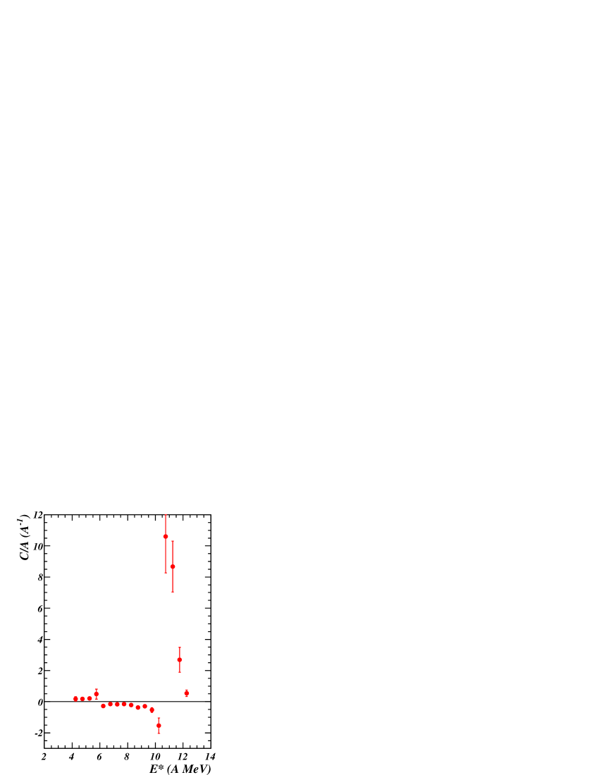
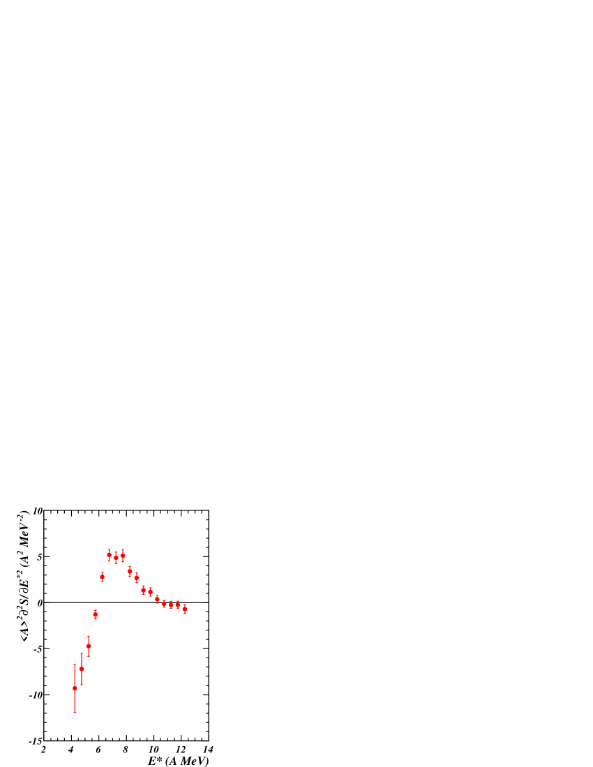
Figure 1: Heat capacity (left) and second derivative of the entropy (right) versus thermal excitation energy $E^{*}$. Error bars correspond to systematic plus statistical errors (see text).

Values of heat capacity and second derivative of the entropy versus thermal excitation energy $E^{*}$ have been calculated respectively from Eqs. (10) and (9) for QF hot nuclei with $Z$ restricted to the range 80-100 to suppress tails of the distributions at different beam energies. The average over the ensemble states have been assimilated to an average over “event ensembles” sorted into $E^{*}$ bins. A binning of 0.5 AMeV was chosen to have a sufficient number of events in each bin in order to reduce statistical errors. Figure 1 shows the results. Error bars correspond to systematic plus statistical errors; systematic errors were evaluated by varying the free parameters of simulations within their limits defined by a $\chi^{2}$ procedure I66-Pia08 . The left part of the figure shows the results for the direct calculation of $C/A$. Negative heat capacity is observed on a rather large thermal excitation energy range and the second diverging region is more visible than the first one.

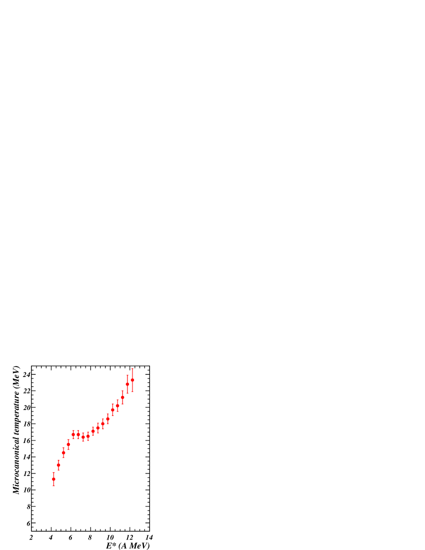
Figure 2: Microcanonical temperatures calculated with Eq. (8). Error bars include systematic plus statistical errors.

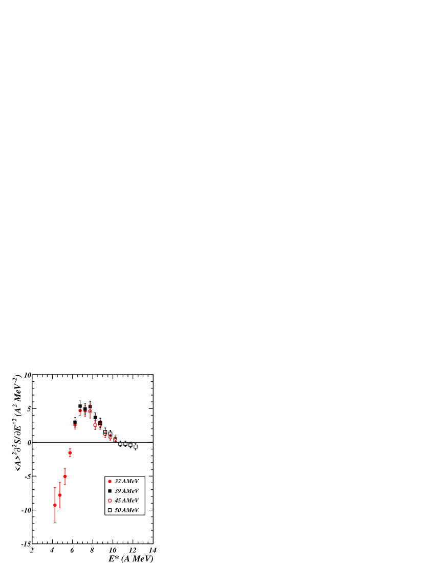
Figure 3: Similar to the right part of fig. 1. The main contributions of the different bombarding energies are shown.

As the second derivative of the entropy is a very small quantity (from $\sim 2.10^{-4}$ to $\sim 3.10^{-6}$), we have kept the presentation made in Radut02 i.e. $A^{2}\partial^{2}S/\partial E^{*2}$ for fig. 1 - right part; A is replaced by the average mass, $<A>$, on the considered $E^{*}$ bin. This quantity, which has small error bars in regions with values close to zero, better defines the $E^{*}$ domain of negative heat capacity. Positive values are measured in the range 6.0 - 10.0 AMeV. The related microcanonical temperatures calculated with Eq. (8) are displayed in fig. 2. Considering the error bars, they are rather constant around 17 - 18 MeV in the $E^{*}$ range where negative heat capacity is observed. With the large multiplicities observed in the present study, microcanonical temperatures are close to classical kinetic temperatures (see figure 3 of I79-Bor13 ). Last point, the statistical nature of the carefully selected event samples, i.e. the independence of the entrance channel, was verified and fig. 3 shows the main contributions of the different bombarding energies to the signal for each $E^{*}$ bin.

Negative heat capacity is thus confirmed for systems with $A$ around 200 without any constraint, which demonstrates once again the robustness of this signal and supports the predictions made in Cho00 i.e. observation at constant pressure or at constant average volume. It is important to stress here that negative heat capacity cannot be observed at constant volume. For the liquid-gas transition in hot nuclei the volume is not fixed but multiplicity and partition-dependent, which means that on the theoretical side one is forced to consider a statistical ensemble for which the volume can fluctuate from event to event around an average value Bor19 .

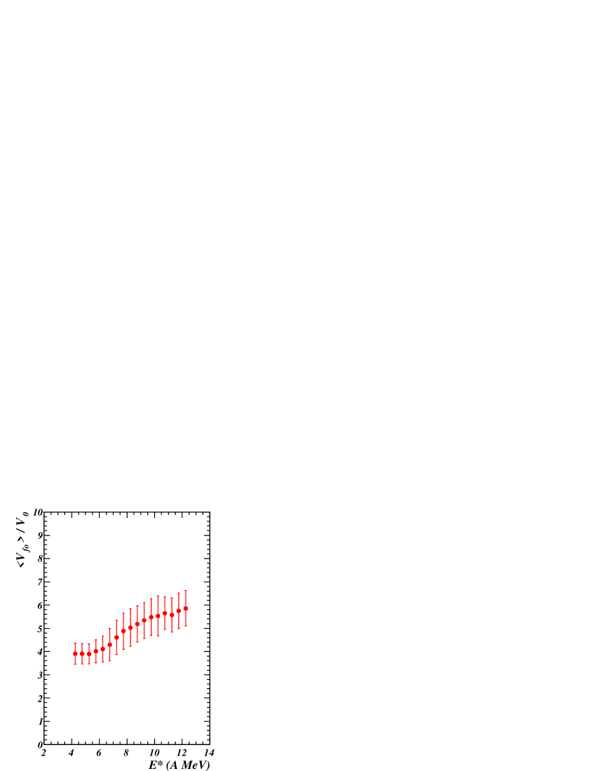
Figure 4: Evolution of the average freeze-out volume of hot nuclei, $V_{fo}$, with thermal excitation energy. Freeze-out volumes are normalized to volumes at saturation density, $V_{0}$, and error bars correspond to standard deviations of $V_{fo}$ distributions.

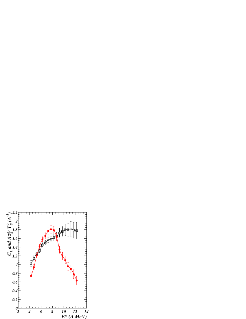
Figure 5: Normalized kinetic energy fluctuations (filled circles) and estimated $C_{k}$ values (open squares) related to the approximate method (see text). Error bars correspond to systematic plus statistical errors.

As compared to previous estimates of heat capacity NicPHD ; I46-Bor02 , there is a significant difference in the $E^{*}$ range for negative values: 6.0$\pm$1.0 - 10.0$\pm$1.0 AMeV in the present study and $<$4.0$\pm$1.0 - 6.0$\pm$1.0 AMeV in the previous one. For quasifusion hot nuclei selection the same shape event sorting was used. The degree of completeness was different (93% here to be compared to 80% before) but it does not affect significantly the thermal excitation energy per nucleon. The method to reconstruct freeze-out properties was also different. But the main difference seems to be related to the average freeze-out volume. In previous estimates the average freeze-out volume was kept constant at 3 times the volume at normal density (3 $V_{0}$) over the whole thermal excitation energy range whereas in the present study it varies from 3.9 to 5.9 $V_{0}$ (see fig. 4). A direct consequence in the approximate method is an increase of Coulomb energy and consequently a decrease and a distortion with excitation energy of $<E_{k}>$ obtained by subtracting the potential part (Coulomb energy + total mass excess) to the thermal energy. To verify this reasoning the approximate method has been used. From our simulation, for each $E^{*}$ bin, we have calculated $<E_{k}>$ (see Eq. (2)) and derived an apparent single temperature, $T_{S}$, needed to build the normalized kinetic energy fluctuations, $A\sigma_{k}^{2}$/$T_{S}^{2}$, to be compared to $C_{k}$ (see Eqs. (3) and (5)). Figure 5 shows that heat capacity becomes negative in the $E^{*}$ range 5.5$\pm$1.0 - 9.0$\pm$1.0 AMeV, i.e. when $A\sigma_{k}^{2}$/$T_{S}^{2}$ overcomes $C_{k}$. This clearly confirms that the main difference, as compared to previous estimates, comes from different average freeze-out volumes. We also note a small decrease of the $E^{*}$ domain as compared to the present study, which possibly comes from the previous method. Last information, the apparent single temperature, $T_{S}$, exhibits a monotonic behaviour, varying from 5.2 to 9.7 MeV over the whole $E^{*}$ range and values increasing from 6.5 to 8 MeV on the domain of negative heat capacity.

In conclusion, heat capacity measurements have been revisited without approximation and by ignoring the hypothesis of a single temperature associated with both internal excitation and thermal motion. For those measurements microcanonical formulae and data reconstructed at freeze-out with the help of a simulation have been used. Negative heat capacity has been confirmed for hot nuclei with $A$ around 200 in the coexistence region of the phase transition.

References

- (1) H. Schulz et al., Phys. Lett. B 119 12 (1982).
- (2) M. W. Curtin et al., Phys. Lett. B 123 219 (1983).
- (3) H. R. Jaqaman et al., Phys. Rev. C 27 2782 (1983).
- (4) H. Müller, B. D Serot, Phys. Rev. C 52 2072 (1995).
- (5) C. Wellenhofer et al., Phys. Rev. C 89 064009 (2014).
- (6) Ph. Chomaz et al. (eds.), Eur. Phys. J. A 30 (2006) and references therein.
- (7) B. Borderie, M.F. Rivet, Prog. Part. Nucl. Phys. 61 551 (2008) and references therein.
- (8) B. Borderie, J.D. Frankland, Prog. Part. Nucl. Phys. 105 82 (2019).
- (9) R. Wada et al., Phys. Rev. C 99 024616 (2019).
- (10) W. Lin et al., Phys. Rev. C 99 054616 (2019).
- (11) P. Labastie et al., Phys. Rev. Lett. 65 1567 (1990).
- (12) D. J. Wales et al., Phys. Rev. Lett. 73 2875 (1994).
- (13) D. H. E. Gross, Phys. Rep. 279 119 (1997).
- (14) F. Gulminelli and Ph. Chomaz, Phys. Rev. E 66 046108 (2002).
- (15) Ph. Chomaz et al., Phys. Rep. 389 263 (2004).
- (16) H. Touchette, Phys. Rep. 478 1 (2009).
- (17) A. Campa et al., Phys. Rep. 480 57 (2009).
- (18) Ph. Chomaz et al., Phys. Rev. Lett. 85 3587 (2000).
- (19) B. Borderie et al. (INDRA Collaboration), Phys. Lett. B 723 140 (2013).
- (20) M. D’Agostino et al., Phys. Lett. B 473 219 (2000).
- (21) N. Le Neindre et al. in Proceedings of the XXXVIII International Winter Meeting on Nuclear Physics, Bormio, Italy, edited by I. Iori and A. Moroni, suppl. 116 (Ricerca Scientifica ed Educazione Permanente, 2000) p. 404.
- (22) B. Borderie, J. Phys. G: Nucl. Part. Phys. 28 R217 (2002).
- (23) N. Le Neindre et al. (INDRA Collaboration), Nucl. Phys. A 795 47 (2007).
- (24) P. Chomaz et al., Phys. Rev. E 64 046114 (2001).
- (25) E. Bonnet et al. (INDRA Collaboration), Phys. Rev. Lett. 103 072701 (2009).
- (26) D.L. Tubbs and S.E. Koonin, Ap. J. 232 L59 (1979).
- (27) D. R. Dean and U. Mosel, Z. Phys. A 322 647 (1985).
- (28) S. E. Koonin, J. Randrup, Nucl. Phys. A 474 173 (1987).
- (29) S. R. Souza et al., Phys. Rev. C 92 024612 (2015).
- (30) S. Piantelli et al. (INDRA Collaboration), Nucl. Phys. A 809 111 (2008).
- (31) Ph. Chomaz and F. Gulminelli, Nucl. Phys. A 647 153 (1999).
- (32) F. Gulminelli et al., Europhys. Lett. 50 434 (2000).
- (33) M. D’Agostino et al., Nucl. Phys. A 699 795 (2002).
- (34) Al. H. Raduta and Ad. R. Raduta, Nucl. Phys. A 703 876 (2002).
- (35) Al. H. Raduta and Ad. R. Raduta, Phys. Rev. C 61 034611 (2000).
- (36) S. Piantelli et al. (INDRA Collaboration), Phys. Lett. B 627 18 (2005).
- (37) E. Bonnet et al. (INDRA Collaboration), Nucl. Phys. A 816 1 (2009).
- (38) J. Pouthas et al., Nucl. Instr. and Meth. in Phys. Res. A 357 418 (1995).
- (39) J. Pouthas et al., Nucl. Instr. and Meth. in Phys. Res. A 369 222 (1996).
- (40) G. Tăbăcaru et al. (INDRA Collaboration), Nucl. Instr. and Meth. in Phys. Res. A 428 379 (1999).
- (41) M. Pârlog et al. (INDRA Collaboration), Nucl. Instr. and Meth. in Phys. Res. A 482 674 (2002).
- (42) M. Pârlog et al. (INDRA Collaboration), Nucl. Instr. and Meth. in Phys. Res. A 482 693 (2002).
- (43) J. D. Frankland et al. (INDRA Collaboration), Nucl. Phys. A 689 940 (2001).
- (44) Y. D. Kim et al., Phys. Rev. C 45 338 (1992).
- (45) G. Tăbăcaru et al. (INDRA Collaboration), Nucl. Phys. A 764 371 (2006).
- (46) S. Shlomo and J.B. Natowitz, Phys. Rev. C 44 2878 (1991).