QPALM: A Proximal Augmented Lagrangian Method for Nonconvex Quadratic Programs

Abstract.

We propose QPALM, a nonconvex quadratic programming (QP) solver based on the proximal augmented Lagrangian method. This method solves a sequence of inner subproblems which can be enforced to be strongly convex and which therefore admit a unique solution. The resulting steps are shown to be equivalent to inexact proximal point iterations on the extended-real-valued cost function, which allows for a fairly simple analysis where convergence to a stationary point at an $R$-linear rate is shown. The QPALM algorithm solves the subproblems iteratively using semismooth Newton directions and an exact linesearch. The former can be computed efficiently in most iterations by making use of suitable factorization update routines, while the latter requires the zero of a monotone, one-dimensional, piecewise affine function. QPALM is implemented in open-source C code, with tailored linear algebra routines for the factorization in a self-written package LADEL. The resulting implementation is shown to be extremely robust in numerical simulations, solving all of the Maros-Meszaros problems and finding a stationary point for most of the nonconvex QPs in the Cutest test set. Furthermore, it is shown to be competitive against state-of-the-art convex QP solvers in typical QPs arising from application domains such as portfolio optimization and model predictive control. As such, QPALM strikes a unique balance between solving both easy and hard problems efficiently.

1. Introduction

This paper considers QPs, namely

$$\operatorname*{minimize}_{x\in\mathbb{R}^{n}}\tfrac{1}{2}x^{\top}Qx+q^{\top}x\quad\operatorname{subject\ to}{}Ax\in C,$$

where $Q\in\mathbb{R}^{n\times n}$ is symmetric, $A\in\mathbb{R}^{m\times n}$, and $C={\mathopen{}\left\{z\in\mathbb{R}^{m}{}\mid{}\ell\leq z\leq u\right\}\mathclose{}}$ for some vectors $\ell,u\in\mathbb{R}^{m}$ is a box. Convex QPs, in which $Q$ is positive semidefinite, are ubiquitous in numerical optimization, as they arise in many applications domains such as portfolio optimization, support vector machines, sparse regressor selection, linear model predictive control (MPC), etc. The solution of a QP is also required in the general nonlinear optimization technique known as sequential quadratic programming (SQP). Therefore, substantial research has been performed to develop robust and efficient QP solvers. State-of-the-art algorithms to solve convex QPs typically fall into one of three categories: active-set methods, interior-point methods or first-order methods.

Active-set methods iteratively determine a working set of active constraints and require the solution of a linear system every time this set changes. Because the change is small however, typically restricted to one or two constraints, the linear system changes only slightly and low-rank factorization updates can be used to make this method efficient. An advantage is that active-set methods can easily make use of an initial guess, also known as a warm-start, which is very useful when solving a series of related QPs, such as in SQP or in MPC. The biggest drawback of active-set methods, however, is that a large number of iterations can be required to converge to the right active set, as the number of possible sets grows exponentially with the number of constraints. Popular active-set-based QP solvers include the open-source solver qpOASES [24] and the QPA module in the open-source software GALAHAD [30].

Interior point methods typically require fewer but more expensive iterations than active-set methods. Their iterations involve the solution of a new linear system at every iteration. Interior-point methods are generally efficient, but suffer from not having warm-starting capabilities. Examples of state-of-the-art QP solvers using an interior-point method are the commercial solvers Gurobi [32] and MOSEK [42], the closed-source solver BPMPD [41] and the open-source solver OOQP [26].

First-order methods rely only on first-order information of the problem. Particularly popular among first-order methods are the proximal algorithms, also known as operator splitting methods. Such methods can typically be described in terms of simple operations, and their iterations are relatively inexpensive. They may, however, exhibit slow asymptotic convergence for ill-conditioned problems. The recently proposed OSQP solver [50], based on the alternating direction method of multipliers (ADMM), addresses this crucial issue somewhat by means of preconditioning.

It is generally difficult to extend the aforementioned methods to be able to find stationary points of nonconvex QPs, without additional assumptions. Augmented-Lagrangian-based algorithms such as the ADMM, for example, would require surjectivity of the constraint matrix $A$ [37, 9, 10, 53]. Some proposals have been made for interior-point methods to solve nonconvex QPs [57, 1], but these methods were found to often exhibit numerical issues in our benchmarks. The active-set solvers SQIC [27] and qpOASES [24] are also able to find critical points of nonconvex QPs and include checks for second-order sufficient conditions to identify local minima. However, the former is not publicly available and the latter is tailored to small-to-medium-scale problems. Finally, global optimization of nonconvex QPs has been the topic of a large amount of research, see for example [49, 11, 12], but this is a separate issue and will not be discussed further here, as we are only interested in finding a stationary point, characterized by the first-order necessary conditions for optimality.

As mentioned in [27, Result 2.1] for instance, the second-order necessary and sufficient condition for optimality requires the positive-definiteness of $Q$ over all feasible directions orthogonal to the local gradient. However, verifying this condition requires finding the global minimizer of an indefinite quadratic form over a cone, which is an NP-hard problem [15]. The authors of [27] propose additionally a necessary (but not sufficient) second-order criterion verifiable in polynomial time, which consists of verifying the positive-definiteness of $Q$ on the nullspace of $A_{\mathcal{I}}$, where $\mathcal{I}$ is the index set of active constraints. This paper restricts itself to considering only first-order conditions, with the exception of using the criterion above a posteriori in the simulations on nonconvex QPs in Section 7.

In this paper we show that the proximal augmented Lagrangian method (P-ALM), up to a simple modification, still enjoys convergence guarantees without convexity or surjectivity assumptions. In particular, this allows us to extend the recently proposed convex QP solver QPALM [33] to nonconvex QPs.

P-ALM when applied to convex problems has been shown to be equivalent to resolvent iterations on the monotone operator encoding the KKT optimality conditions [46]. While this interpretation is still valid for (1) under our working assumptions, the resulting KKT system lacks the monotonicity requirement that is needed for guaranteeing convergence of the iterates. In fact, while $\mathcal{M}$ is hypo-monotone, in the sense that it can be made monotone by adding a suitably large multiple of the identity mapping, the same cannot be said about its inverse $\mathcal{M}^{-1}$ whence recent advancements in the nonconvex literature would apply, see [34, 14]. For this reason, we here propose a different interpretation of a P-ALM step as an inexact proximal point iteration on the extended-real-valued cost

$$\varphi(x){}\coloneqq{}\tfrac{1}{2}x^{\top}Qx+q^{\top}x+\operatorname{\delta}_{C}(Ax),$$

where $\operatorname{\delta}_{C}$ is the indicator function of set $C$, namely $\operatorname{\delta}_{C}(x)=0$ if $x\in C$ and $\infty$ otherwise. As will be better detailed in Section 2, the proximal point (PP) subproblems are addressed by means of an ALM method where the hard constraint $Ax\in C$ is replaced by a quadratic penalty, overall resulting in the proposed proximal-ALM method for quadratic programs QPALM.

Some recent papers [36, 38] developed and analyzed the iteration complexity of a closely related three-layer algorithm, not specifically for QPs, which involves solving a series of quadratically penalized subproblems using inexact proximal point iterations. Although dealing with nonconvexity in the objective through the proximal penalty as well, the approach is quite different from ours in that it uses a pure quadratic penalty instead of ALM, and thus requires the penalty parameters to go to infinity and is prone to exhibit slower convergence rates [6, §2.2.5]. Furthermore, the inner subproblems are solved using an accelerated (first-order) composite gradient method, whereas QPALM uses a semismooth Newton method. Finally, to the best of our knowledge, no code for their algorithm was provided.

1.1. Contributions

Our contributions can be summarized as follows.

1. We show the equivalence between P-ALM and PP iterations, and more specifically the relation between the inexactness in both methods. As such, we can make use of the convergence results of [51, §4.1]. In addition, we show that inexact PP on possibly nonconvex QPs is globally convergent and, in fact, with $R$-linear rates, thus complementing [39, Prop. 3.3] that covers the exact case.

2. We modify the QPALM algorithm introduced in a previous paper for convex QPs [33], such that it can now also deal with nonconvex QPs. We highlight the (minimal) changes required, and add a self-written C version of the LO(B)PCG algorithm, used to find the minimum eigenvalue, to the QPALM source code.

3. We outline the necessary linear algebra routines and present a standalone C package LADEL that implements them. Therefore, differently from our previous version which relied on CHOLMOD [13], QPALM is now a standalone software package. Furthermore, all the details of the parameter selection and initialization routines are outlined here.

4. We provide extensive benchmarking results, not only for nonconvex QPs which we obtain from the Cutest test set [31], but also for convex QPs. Here, we vastly extend the limited results presented in [33] by solving the Maros-Meszaros problems, many of which are large scale and ill conditioned, alongside some QPs arising from specific application domains, such as portfolio optimization and model predictive control.

1.2. Notation

The following notation is used throughout the paper. We denote the extended real line by $\overline{\mathbb{R}}\coloneqq\mathbb{R}\cup{\mathopen{}\left\{\infty{}\mid{}{}\right\}\mathclose{}}$. The scalar product on $\mathbb{R}^{n}$ is denoted by $\langle{}{}\cdot{}{},{}{}\cdot{}{}\rangle$. With $[x]_{+}\coloneqq\max{\mathopen{}\left\{x,0{}\mid{}{}\right\}\mathclose{}}$ we indicate the positive part of vector $x\in\mathbb{R}^{n}$, meant in a componentwise sense. A sequence of vectors $(x^{k})_{k\in\mathbb{N}}$ is said to be summable if $\sum_{k\in\mathbb{N}}\|x^{k}\|<\infty$.

With $\operatorname{Sym}(\mathbb{R}^{n})$ we indicate the set of symmetric $\mathbb{R}^{n\times n}$ matrices, while $\operatorname{Sym}_{+}(\mathbb{R}^{n})$ and $\operatorname{Sym}_{++}(\mathbb{R}^{n})$ denote the subsets of those which are positive semidefinite and positive definite, respectively. For two matrices $A,B\in\operatorname{Sym}(\mathbb{R}^{n})$ we write $A\succeq B$ (resp. $A\succ B$) to indicate that $A-B$ is positive semidefinite (resp. positive definite), and given $\Sigma\in\operatorname{Sym}_{++}(\mathbb{R}^{n})$ we indicate with $\|{}\cdot{}\|_{\Sigma}$ the norm on $\mathbb{R}^{n}$ induced by $\Sigma$, namely $\|x\|_{\Sigma}{}\coloneqq{}\sqrt{\langle{}x{},{}\Sigma x{}\rangle}$. With $I_{n}$ we denote the $n\times n$-identity matrix, and we simply write $I$ when $n$ is clear from context.

Given a nonempty closed convex set $C\subseteq\mathbb{R}^{n}$, with $\operatorname{\Pi}_{C}(x)$ we indicate the projection of a point $x\in\mathbb{R}^{n}$ onto $C$, namely $\operatorname{\Pi}_{C}(x)=\operatorname*{arg\,min}_{y\in C}\|y-x\|$ or, equivalently, the unique point $z\in C$ satisfying the inclusion

$$x-z\in\operatorname{\mathcal{N}}_{C}(z),$$ (1.1)

where $\operatorname{\mathcal{N}}_{C}(z){}\coloneqq{}{\mathopen{}\left\{v\in\mathbb{R}^{n}{}\mid{}\langle{}v{},{}z-z^{\prime}{}\rangle\leq 0\leavevmode\nobreak\ \forall z^{\prime}\in C\right\}\mathclose{}}$ is the normal cone of the set $C$ at $z$. $\operatorname{dist}(x,C)$ and $\operatorname{dist}_{\Sigma}(x,C)$ denote the distance from $x$ to set $C$ in the Euclidean norm and in that induced by $\Sigma$, respectively, while $\operatorname{\delta}_{C}$ is the indicator function of set $C$, namely $\operatorname{\delta}_{C}(x)=0$ if $x\in C$ and $\infty$ otherwise. For a set of natural numbers $\mathcal{I}\in\mathbb{N}$ we let $|\mathcal{I}|$ denote its cardinality, whereas for a (sparse) matrix $A\in\mathbb{R}^{m\times n}$ we let $|A|$ denote the number of nonzero elements in $A$. The element of $A$ in the $i$-th row and $j$-th column is denoted as $A_{ij}\in\mathbb{R}$. For an index $i\in[1,m]$, let $A_{i\cdot}$ denote the $i-$th row of $A$. Similarly, for a set of indices $\mathcal{I}\subseteq[1,m]$, let $A_{\text{\tiny{$\mathcal{I}\cdot$}}}\in\mathbb{R}^{|\mathcal{I}|\times n}$ be the submatrix comprised of all the rows $i\in\mathcal{I}$ of $A$. Analogously, for $j\in[1,n]$, and $\mathcal{J}\subseteq[1,n]$, let $A_{\cdot j}$ denote the $j$-th column of $A$, and $A_{\text{\tiny{$\cdot\mathcal{J}$}}}$ the submatrix comprised of all the columns $j\in\mathcal{J}$ of $A$. Combined, let $A_{\text{\tiny{$\mathcal{I}\mathcal{J}$}}}\in\mathbb{R}^{|\mathcal{I}|\times|\mathcal{J}|}$ denote the submatrix comprised of all the rows $i\in\mathcal{I}$ and all the columns $j\in\mathcal{J}$ of $A$. Finally, let us denote the matrix $A^{\text{\tiny{$\mathcal{I}\cdot$}}}\in\mathbb{R}^{m\times n}$ as the matrix with the corresponding rows from $A$ and $\mathbf{0}$ elsewhere, i.e.

$${A_{i\cdot}^{\text{\tiny{$\mathcal{I}$}}}={\mathopen{}\left\{\begin{array}[]{l @{~~} >{\text{if~}}l<{\text{,}} }A_{i\cdot}\hfil\leavevmode\nobreak\ \leavevmode\nobreak\ &\leavevmode\nobreak\ }i\in\mathcal{I}\\ \mathbf{0}\hfil\leavevmode\nobreak\ \leavevmode\nobreak\ &\lx@intercol\text{otherwise,}\hfil\lx@intercol\end{array}\right.\mathclose{}}$$

and similarly $A^{\text{\tiny{$\mathcal{I}\mathcal{J}$}}}\in\mathbb{R}^{m\times n}$ the matrix with elements

$${A_{ij}^{\text{\tiny{$\mathcal{I}\mathcal{J}$}}}={\mathopen{}\left\{\begin{array}[]{l @{~~} >{\text{if~}}l<{\text{,}} }A_{ij}\hfil\leavevmode\nobreak\ \leavevmode\nobreak\ &\leavevmode\nobreak\ }i\in\mathcal{I}\textrm{ and }j\in\mathcal{J}\\ 0\hfil\leavevmode\nobreak\ \leavevmode\nobreak\ &\lx@intercol\text{otherwise.}\hfil\lx@intercol\end{array}\right.\mathclose{}}$$

A mapping $F:\mathbb{R}^{n}\rightarrow\mathbb{R}^{m}$ is Lipschitz continuous on $\Omega\subseteq\mathbb{R}^{n}$ if there exists $L\geq 0$ such that $\|F(x)-F(y)\|\leq L\|x-y\|$ holds for all $x,y\in\Omega$. The smallest such constant $L$ is the Lipschitz modulus of $F$ on $\Omega$, denoted as $\operatorname{lip}_{\Omega}F$ or simply $\operatorname{lip}F$ when $\Omega=\mathbb{R}^{n}$. We say that a real-valued function $h:\mathbb{R}^{n}\rightarrow\mathbb{R}$ is Lipschitz differentiable if $h$ is continuosly differentiable and its gradient ${\nabla}h$ is Lipschitz continuous on $\mathbb{R}^{n}$. We may also say that $h$ is $L_{h}$-smooth as a shorthand notation to indicate that $h$ is Lipschitz differentiable with $\operatorname{lip}{\nabla}h=L_{h}$.

For an extended-real-valued function $f:\mathbb{R}^{n}\rightarrow\overline{\mathbb{R}}$ and $\alpha\in\mathbb{R}$ we indicate with $\operatorname{lev}_{\leq\alpha}f{}\coloneqq{}{\mathopen{}\left\{x\in\mathbb{R}^{n}{}\mid{}f(x)\leq\alpha\right\}\mathclose{}}$ the $\alpha$-sublevel set of $f$, and we say that $f$ is level bounded if $\operatorname{lev}_{\leq\alpha}f$ is a bounded set for any $\alpha\in\mathbb{R}$, this condition being equivalent to $\lim_{\|x\|\to\infty}f(x)=\infty$.

1.3. Nonconvex subdifferential and proximal mapping

The regular subdifferential of $f:\mathbb{R}^{n}\rightarrow\overline{\mathbb{R}}$ at $x\in\mathbb{R}^{n}$ is the set $\hat{\partial}f(x)$, where

$$v\in\hat{\partial}f(x)\quad\text{iff}\quad\liminf_{x^{\prime}\to x}\frac{f(x^{\prime})-f(x)-\langle{}v{},{}x^{\prime}-x{}\rangle}{\|x^{\prime}-x\|}{}\geq{}0,$$

whereas the (limiting) subdifferential of $f$ at $x$ is $\partial f(x)=\emptyset$ if $x\notin\operatorname{dom}f$, and

$$\partial f(x){}\coloneqq{}{\mathopen{}\left\{v\in\mathbb{R}^{n}{}\mid{}\exists(x^{k},v^{k})\to(x,v)\leavevmode\nobreak\ \text{such that}\leavevmode\nobreak\ f(x^{k})\to f(x)\leavevmode\nobreak\ \text{and}\leavevmode\nobreak\ v^{k}\in\hat{\partial}f(x^{k})\leavevmode\nobreak\ \forall k\right\}\mathclose{}}$$

otherwise. Notice that $\hat{\partial}f(x)\subseteq\partial f(x)$ for any $x\in\mathbb{R}^{n}$, and that the inclusion $0\in\hat{\partial}f(x)$ is a necessary condition for local minimality of $x$ for $f$ [47, Thm.s 8.6 and 10.1]. A point $x$ satisfying this inclusion is said to be stationary (for $f$). If $f$ is proper lower semicontinuous (lsc) and convex, then

$$\hat{\partial}f(x){}={}\partial f(x){}={}{\mathopen{}\left\{v\in\mathbb{R}^{n}{}\mid{}f(x^{\prime})\geq f(x)+\langle{}v{},{}x^{\prime}-x{}\rangle\leavevmode\nobreak\ \forall x^{\prime}\in\mathbb{R}^{n}\right\}\mathclose{}},$$

and stationarity of $x$ for $f$ is a necessary and sufficient condition for global minimality [47, Prop. 8.12 and Thm. 10.1]. For a proper lsc function $f$ and $\Sigma_{\text{\sf{x}}}\in\operatorname{Sym}_{++}(\mathbb{R}^{n})$, the proximal mapping of $f$ with (matrix) stepsize $\Sigma_{\text{\sf{x}}}$ is the set-valued mapping $\operatorname{prox}_{f}^{\Sigma_{\text{\sf{x}}}}:\mathbb{R}^{n}\rightrightarrows\mathbb{R}^{n}$ given by

$$\operatorname{prox}_{f}^{\Sigma_{\text{\sf{x}}}}(x){}\coloneqq{} \operatorname*{arg\,min}_{w\in\mathbb{R}^{n}}{\mathopen{}\left\{f(w){}+{}\tfrac{1}{2}\|w-x\|_{\Sigma_{\text{\sf{x}}}^{-1}}^{2}{}\mid{}{}\right\}\mathclose{}},$$

and the corresponding Moreau envelope is $$f^{\Sigma_{\text{\sf{x}}}}:\mathbb{R}^{n}\rightarrow\mathbb{R}$$ defined as

$$f^{\Sigma_{\text{\sf{x}}}}(x){}\coloneqq{} \min_{w\in\mathbb{R}^{n}}{\mathopen{}\left\{f(w){}+{}\tfrac{1}{2}\|w-x\|_{\Sigma_{\text{\sf{x}}}^{-1}}^{2}{}\mid{}{}\right\}\mathclose{}}.$$

It follows from the definition that $\bar{x}\in\operatorname{prox}_{f}^{\Sigma_{\text{\sf{x}}}}(x)$ iff

$$f^{\Sigma_{\text{\sf{x}}}}(x){}={}f(\bar{x}){}+{}\tfrac{1}{2}\|x-\bar{x}\|_{\Sigma_{\text{\sf{x}}}^{-1}}^{2}{}\leq{}f(x^{\prime}){}+{}\tfrac{1}{2}\|x-x^{\prime}\|_{\Sigma_{\text{\sf{x}}}^{-1}}^{2}\quad\forall x^{\prime}\in\mathbb{R}^{n}.$$ (1.2)

Moreover, for every $x\in\mathbb{R}^{n}$ it holds that

$$\Sigma_{\text{\sf{x}}}^{-1}(x-\bar{x}){}\in{}\hat{\partial}f(\bar{x}),\quad\text{where}\quad\bar{x}{}\in{}\operatorname{prox}_{f}^{\Sigma_{\text{\sf{x}}}}(x).$$ (1.3)

If $\Sigma_{\text{\sf{x}}}$ is such that $f+\tfrac{1}{2}\|{}\cdot{}\|_{\Sigma_{\text{\sf{x}}}^{-1}}^{2}$ is strongly convex (in which case $f$ is said to be hypoconvex), then $\operatorname{prox}_{f}^{\Sigma_{\text{\sf{x}}}}$ is (single-valued and) Lipschitz continuous and $f^{\Sigma_{\text{\sf{x}}}}$ Lipschitz differentiable, and (1.3) can be strenghtened to

$${\nabla}f^{\Sigma_{\text{\sf{x}}}}(x){}={}\Sigma_{\text{\sf{x}}}^{-1}(x-\bar{x}){}\in{}\hat{\partial}f(\bar{x}),\quad\text{where}\quad\bar{x}{}={}\operatorname{prox}_{f}^{\Sigma_{\text{\sf{x}}}}(x).$$ (1.4)

1.4. Paper outline

The remainder of the paper is outlined as follows. Section 2 discusses the theoretical convergence of inexact proximal point iterations on the extended-real-valued cost of (1), and shows equivalence between these iterations and the inexact proximal augmented Lagrangian method. Algorithm 1 therein illustrates the proposed (modification of) proximal ALM applied to QPs, thus providing a snapshot of the main steps of the proposed QPALM algorithm pruned of all the implementation details, which will instead be covered in the subsequent sections. Specifically, Section 3 deals with the inner minimization procedure required at 1.3, that is, the semismooth Newton method with exact linesearch of [33]. Section 4 covers the required heavy duty linear algebra routines, including factorizations and factorization updates, and the LO(B)PCG algorithm used to compute the minimum eigenvalue of $Q$. Section 5 lays out in detail the parameters used in QPALM, how they are initialized and updated. It furthermore discusses preconditioning of the problem data, as well as termination criteria and infeasibility detection routines. After a brief recap on the material of the previous sections, Section 6 presents the fully detailed implementation of QPALM in the dedicated Algorithm 7, together with a comprehensive overview of all the algorithmic steps therein. Section 7 then presents numerical results obtained by comparing this implementation against state-of-the-art solvers. Finally, Section 8 draws the concluding remarks of the paper.

2. Proximal ALM

As mentioned in the introduction, our methodology revolves around the interpretation of a P-ALM step on (1) as an inexact proximal point iteration on the extended-real-valued cost

$$\varphi(x){}\coloneqq{}\tfrac{1}{2}x^{\top}Qx+q^{\top}x+\operatorname{\delta}_{C}(Ax),$$ (2.1)

namely

$$\hat{x}^{k+1}{}\approx{}\operatorname{prox}_{\varphi}^{\Sigma_{\text{\sf{x}}}}(\hat{x}^{k}){}\coloneqq{}\operatorname*{arg\,min}_{x\in\mathbb{R}^{n}}{\mathopen{}\left\{\varphi(x)+\tfrac{1}{2}\|x-\hat{x}^{k}\|_{\Sigma_{\text{\sf{x}}}^{-1}}^{2}{}\mid{}{}\right\}\mathclose{}}.$$ (2.2)

Although differing from the original (1) only by a quadratic term, similarly to what suggested in [5] by selecting a suitably small weight $\Sigma_{\text{\sf{x}}}\in\operatorname{Sym}_{++}(\mathbb{R}^{n})$ this minimization subproblem can be made strongly convex and addressed by means of an ALM method where the hard constraint $Ax\in C$ is replaced by a quadratic penalty. Note that, in order to make the subproblem strongly convex, a diagonal matrix $\Sigma_{\text{\sf{x}}}$ can be chosen based on the minimum eigenvalue $\lambda_{\rm min}$ of the objective Hessian matrix $Q$. If $\lambda_{\rm min}\geq 0$, corresponding to a convex QP, then any positive definite $\Sigma_{\text{\sf{x}}}$ works; otherwise, it is easy to verify that it is enough to select the diagonal elements as $0<\Sigma_{\text{\sf{x}},ii}<-\nicefrac{{1}}{{\lambda_{\rm min}}}$, and that $\lambda_{\rm min}$ can be replaced by any (under-)estimation carried out at initialization.

Using ALM to solve the inner PP subproblems gives rise to a modification of the proximal ALM scheme, the difference being that the proximity point $\hat{x}^{k}$ is kept constant for some subsequent iterations until a suitably accurate solution $\hat{x}^{k+1}$ of (2.2) has been found. This subproblem amounts to the nonsmooth composite minimization

$$\operatorname*{minimize}_{x\in\mathbb{R}^{n},z\in\mathbb{R}^{m}}f(x)+g(z)+\tfrac{1}{2}\|x-\hat{x}^{k}\|_{\Sigma_{\text{\sf{x}}}^{-1}}^{2}\quad\operatorname{subject\ to}{}Ax-z=0,$$ (2.3)

where $f=\tfrac{1}{2}\langle{}{}\cdot{}{},{}Q{}\cdot{}{}\rangle+\langle{}q{},{}{}\cdot{}{}\rangle$ and $g=\operatorname{\delta}_{C}$, and thus itself requires an iterative procedure.

Starting from a vector $$y^{k}\in\mathbb{R}^{m} \Sigma_{\text{\sf{y}},k}\in\operatorname{Sym}_{++}(\mathbb{R}^{m}) (x^{k+1},z^{k+1},y^{k+1})$$ and for a given dual weight matrix , one iteration of ALM applied to (2.3) produces a triplet according to the following update rule:

$${\mathopen{}\left\{\begin{array}[]{r @{{}={}} l}(x^{k+1},z^{k+1})&\operatorname*{arg\,min}_{x,z}\mathcal{L}_{\hat{x}^{k},\Sigma_{\text{\sf{x}}},\Sigma_{\text{\sf{y}},k}}(x,z,y^{k})\\[3.0pt] y^{k+1}&y^{k}{}+{}\Sigma_{\text{\sf{y}},k}(Ax^{k+1}-z^{k+1}),\end{array}\right.\mathclose{}}$$ (2.4a)

where

$$\mathcal{L}_{\hat{x}^{k},\Sigma_{\text{\sf{x}}},\Sigma_{\text{\sf{y}}}}(x,z,y){}\coloneqq{}f(x){}+{}\tfrac{1}{2}\|x-\hat{x}^{k}\|_{\Sigma_{\text{\sf{x}}}^{-1}}^{2}{}+{}g(z){}+{}\langle{}y{},{}Ax-z{}\rangle{}+{}\tfrac{1}{2}\|Ax-z\|_{\Sigma_{\text{\sf{y}}}}^{2}$$ (2.4b)

is the $$\Sigma_{\text{\sf{y}}}$$-augmented Lagrangian associated to (2.3).

Notice that, by first minimizing with respect to $z$, apparently $x^{k+1}$ and $z^{k+1}$ are given by

$${\mathopen{}\left\{\begin{array}[]{r @{{}={}} l}x^{k+1}&\operatorname*{arg\,min}_{x\in\mathbb{R}^{n}}{\mathopen{}\left\{f(x){}+{}g^{\Sigma_{\text{\sf{y}},k}^{-1}}(Ax+\Sigma_{\text{\sf{y}},k}^{-1}y^{k}){}+{}\tfrac{1}{2}\|x-\hat{x}^{k}\|_{\Sigma_{\text{\sf{x}}}^{-1}}^{2}{}\mid{}{}\right\}\mathclose{}}\\ z^{k+1}&\operatorname{prox}_{g}^{\Sigma_{\text{\sf{y}},k}^{-1}}(Ax^{k+1}+\Sigma_{\text{\sf{y}},k}^{-1}y^{k}){}={}\operatorname{\Pi}_{C}(Ax^{k+1}+\Sigma_{\text{\sf{y}},k}^{-1}y^{k}),\end{array}\right.\mathclose{}}$$ (2.5)

where the second equality in the $z$-update owes to the fact that $C$ is a box and $\Sigma_{\text{\sf{y}},k}$ is diagonal, so that the projections onto $C$ with respect to $\|{}\cdot{}\|$ and $\|{}\cdot{}\|_{\Sigma_{\text{\sf{y}},k}^{-1}}$ coincide.

Remark 2.1 (Proximal ALM vs plain ALM).

A major advantage of proximal ALM over plain ALM when applied to a nonconvex QP is that by suitably selecting the proximal weights each subproblem is guaranteed to have solutions. An illustrative example showing how ALM may not be applicable is given by the nonconvex QP

$$\operatorname*{minimize}_{x\in\mathbb{R}^{2}}x_{1}x_{2}\quad\operatorname{subject\ to}x_{1}=0,$$

which is clearly lower bounded and with minimizers given by ${\mathopen{}\left\{x\in\mathbb{R}^{2}{}\mid{}x_{1}=0\right\}\mathclose{}}$. For a fixed penalty $\beta>0$ and a Lagrangian multiplier $y\in\mathbb{R}$, the $x$-minimization step prescribed by ALM is

$$x_{\rm ALM}^{+}{}\in{}\operatorname*{arg\,min}_{w\in\mathbb{R}^{2}}{\mathopen{}\left\{w_{1}w_{2}{}+{}\langle{}y{},{}w_{1}{}\rangle{}+{}\tfrac{\beta}{2}\|w_{1}\|^{2}{}\mid{}{}\right\}\mathclose{}}{}={}\emptyset,$$

owing to lower unboundedness of the augmented Lagrangian (take, e.g., $w^{k}=(1,-k)$ for $k\to\infty$). The problem is readily solved by proximal ALM, as long as the proximal weight $\Sigma_{\text{\sf{x}}}\in\operatorname{Sym}_{++}(\mathbb{R}^{2})$ satisfies $\Sigma_{\text{\sf{x}}}\prec I_{2}$ (the $2\times 2$-identity matrix). In fact, the P-ALM update step results in

$$x_{\text{\rm P-ALM}}^{+}{}\in{}\operatorname*{arg\,min}_{w\in\mathbb{R}^{2}}{\mathopen{}\left\{w_{1}w_{2}{}+{}\langle{}y{},{}w_{1}{}\rangle{}+{}\tfrac{\beta}{2}\|w_{1}\|^{2}{}+{}\tfrac{1}{2}\|w-x\|_{\Sigma_{\text{\sf{x}}}^{-1}}^{2}{}\mid{}{}\right\}\mathclose{}}\\ {}={}{\mathopen{}\left\{\textstyle\Bigl{[}\Sigma_{\text{\sf{x}}}^{-1}{}+{}\binom{\beta\leavevmode\nobreak\ \leavevmode\nobreak\ 1}{1\leavevmode\nobreak\ \leavevmode\nobreak\ \hphantom{\beta}}\Bigr{]}^{-1}\Bigl{(}\Sigma_{\text{\sf{x}}}x{}-{}\binom{y}{0}\Bigr{)}{}\mid{}{}\right\}\mathclose{}},$$

which is well defined for any Lagrange multiplier $y$ and penalty $\beta>0$. ∎

The resulting proximal ALM is outlined in Algorithm 1. The iterate $x^{k+1}$ retrieved at 1.3 corresponds to an approximate solution of the smooth $x$-subproblem in (2.5) which, in principle, can be carried out by any smooth minimization technique terminating when the norm of the gradient falls within the prescribed tolerance $\delta_{k}$. The proposed QPALM solver, whose full implementation is outlined in Algorithm 7 in Section 6, will ultimately address this step with a semismooth Newton method with exact linesearch. For the moment being, however, we shall regard this update as a black box to merely focus on the convergence analysis of the outer proximal ALM.

Algorithm 1 Proximal augmented Lagrangian method for nonconvex QPs

1.1:   

$(\hat{x}^{0},y^{0})\in\mathbb{R}^{n}\times\mathbb{R}^{m}$;   $\delta_{0},\varepsilon_{0}>0$;   $\rho\in(0,1)$;   $\Sigma_{\text{\sf{y}},0}\succeq\Sigma_{\text{\sf{y}},\rm min}\in\operatorname{Sym}_{++}(\mathbb{R}^{m})$

$\Sigma_{\text{\sf{x}}}\in\operatorname{Sym}_{++}(\mathbb{R}^{n})$  such that  $Q+\Sigma_{\text{\sf{x}}}^{-1}\succ 0$

1.2:   for  $k=0,1,\ldots$  do

1.3:       

Let $x^{k+1}$ be such that  $\Bigl{\|}\leavevmode\nobreak\ \smash{\vphantom{Qx^{k+1}{}+{}q}\smash{\overbrace{Qx^{k+1}{}+{}q}^{{\nabla}f(x^{k+1})}}{}+{}\vphantom{\Sigma_{\text{\sf{y}},k}(Ax^{k+1}-z^{k+1})+y^{k}}\smash{\overbrace{\Sigma_{\text{\sf{y}},k}(Ax^{k+1}-z^{k+1})+y^{k}}^{{\nabla}g^{\Sigma_{\text{\sf{y}},k}^{-1}}(x^{k+1})}}{}+{}\Sigma_{\text{\sf{x}}}^{-1}(x^{k+1}-\hat{x}^{k})}\leavevmode\nobreak\ \Bigr{\|}{}\leq{}\delta_{k}$

where $z^{k+1}{}={}\operatorname{\Pi}_{C}\bigl{(}Ax^{k+1}+\Sigma_{\text{\sf{y}},k}^{-1}y^{k}\bigr{)}$

1.4:       $y^{k+1}{}={}y^{k}{}+{}\Sigma_{\text{\sf{y}},k}(Ax^{k+1}-z^{k+1})$

1.5:       if  $\|Ax^{k+1}-z^{k+1}\|_{\Sigma_{\text{\sf{y}},k}}\leq\varepsilon_{k}$  then$\triangleright$ [Quit ALM inner loop]

1.6:           Update $\hat{x}^{k+1}=x^{k+1}$  and choose  $\Sigma_{\text{\sf{y}},k+1}\succeq\Sigma_{\text{\sf{y}},\rm min}$ and $\varepsilon_{k+1}\leq\rho\varepsilon_{k}$

1.7:       else

1.8:           Set  $\hat{x}^{k+1}=\hat{x}^{k}$ and $\varepsilon_{k+1}=\varepsilon_{k}$,  and choose  $\Sigma_{\text{\sf{y}},k+1}\succeq\Sigma_{\text{\sf{y}},k}$     

1.9:       Choose $\delta_{k+1}\leq\rho\delta_{k}$

2.1. Inexact proximal point

We now summarize a key result that was shown in [51, §4.1] in the more general setting of proximal gradient iterations. Given that [51] has not yet been peer-reviewed and also for the sake of self-containedness, we provide a proof tailored to our simplified setting in the dedicated Section A.

Theorem 2.2 (Inexact nonconvex PP [51, §4.1]).

Let $\varphi:\mathbb{R}^{n}\rightarrow\overline{\mathbb{R}}$ be a proper, lsc and lower bounded function. Starting from $x^{0}\in\mathbb{R}^{n}$ and given a sequence $(e^{k})_{k\in\mathbb{N}}\subset\mathbb{R}^{n}$ such that $\sum_{k\in\mathbb{N}}\|e^{k}\|<\infty$, consider the inexact PP iterations

$$x^{k+1}{}\in{}\operatorname{prox}_{\varphi}^{\Sigma_{\text{\sf{x}}}}(x^{k}+e^{k})$$

for some $\Sigma_{\text{\sf{x}}}\in\operatorname{Sym}_{++}(\mathbb{R}^{n})$. Then, the following hold:

1. the real-valued sequence $(\varphi(x^{k+1}))_{k\in\mathbb{N}}$ converges to a finite value;

2. the sequence $(\|x^{k+1}-x^{k}\|^{2})_{k\in\mathbb{N}}$ has finite sum, and in particular $\min_{i\leq k}\|x^{k+1}-x^{i}\|\leq o(\nicefrac{{1}}{{\sqrt{k}}})$;

3. $\varphi$ is constant and equals the limit of $(\varphi(x^{k+1}))_{k\in\mathbb{N}}$ on the set of cluster points of $(x^{k})_{k\in\mathbb{N}}$, which is made of stationary points for $\varphi$;

4. if $\varphi$ is coercive, then $(x^{k})_{k\in\mathbb{N}}$ is bounded.

See Section A.

We remark that with trivial modifications of the proof the arguments also apply to time-varying proximal weights $\Sigma_{\text{\sf{x}},k}$, $k\in\mathbb{N}$, as long as there exist $\Sigma_{\text{\sf{x}},\rm min},\Sigma_{\text{\sf{x}},\rm max}\in\operatorname{Sym}_{++}(\mathbb{R}^{n})$ such that $\Sigma_{\text{\sf{x}},\rm min}\preceq\Sigma_{\text{\sf{x}},k}\preceq\Sigma_{\text{\sf{x}},\rm max}$ holds for all $k$. Item 4 indicates that coerciveness of the cost function is a sufficient condition for inferring boundedness of the iterates. In (1), however, the cost function $\varphi$ may fail to be coercive even if lower bounded on the feasible set ${\mathopen{}\left\{x{}\mid{}Ax\in C\right\}\mathclose{}}$. This happens when there is a feasible direction for which the objective is constant, i.e., when $\lim_{\tau\to\infty}\operatorname{\delta}_{C}(A(x+\tau d))=0$, $Qd=0$ and $q^{\top}d=0$ hold for some $x,d\in\mathbb{R}^{n}$ with $d\neq 0$. Nevertheless, it has been shown in [39] that (exact) proximal point iterations on a lower bounded nonconvex quadratic program remain bounded and, in fact, converge to a stationary point. We next show that this remains true even for inexact proximal point iterations, provided that the inexactness vanishes at linear rate. The proof hinges on the (exact) proximal gradient error bound analysis of [39] and on the close relation existing among proximal point and proximal gradient iterations for this kind of problems. Before showing the result in Theorem 2.5, we present a simple technical lemma that will be needed in the proof.

Lemma 2.3.

Let $h$ be a lower bounded and $L_{h}$-smooth function. Then, for every $\alpha>0$ it holds that

$$\operatorname{lip}_{\operatorname{lev}_{\leq\inf h+\alpha}h}h{}\leq{}\tfrac{1+\sqrt{2}}{2}\sqrt{2\alpha L_{h}}.$$

Without loss of generality we may assume that $\inf h=0$. Let $\alpha>0$ be fixed, and consider $x,y\in\operatorname{lev}_{\leq\alpha}h$ with $x\neq y$. From the quadratic upper bound of Lipschitz differentiable functions (see e.g., [7, Prop. A.24]) and the fact that $0\leq h(x),h(y)\leq\alpha$ we have that

$$\frac{|h(y)-h(x)|}{\|y-x\|}{}\leq{}\min{\mathopen{}\left\{\tfrac{\alpha}{\|y-x\|},\,\|{\nabla}h(x)\|+\tfrac{L_{h}}{2}\|y-x\|{}\mid{}{}\right\}\mathclose{}}\\ {}\leq{}\min{\mathopen{}\left\{\tfrac{\alpha}{\|y-x\|},\,\sqrt{2\alpha L_{h}}+\tfrac{L_{h}}{2}\|y-x\|{}\mid{}{}\right\}\mathclose{}},$$ (2.6)

where the last inequality follows from the fact that

$$\alpha{}\geq{}h(x)-h(x-\tfrac{1}{L_{h}}{\nabla}h(x)){}\geq{}\tfrac{1}{2L_{h}}\|{\nabla}h(x)\|^{2},$$

where the last equality again uses the quadratic lower bound of [7, Prop. A.24]. By solving a second-order equation in $\|y-x\|$, we see that

$$\min{\mathopen{}\left\{\tfrac{\alpha}{\|y-x\|},\sqrt{2\alpha L_{h}}+\tfrac{L_{h}}{2}\|y-x\|{}\mid{}{}\right\}\mathclose{}}{}={} {\displaystyle{\mathopen{}\left\{\begin{array}[]{l @{~~} >{\text{if~}}l<{\text{,}} }\tfrac{\alpha}{\|y-x\|}\hfil\leavevmode\nobreak\ \leavevmode\nobreak\ &\leavevmode\nobreak\ }\|y-x\|{}\geq{}(2-\sqrt{2})\sqrt{\frac{\alpha}{L_{h}}}\\ \sqrt{2\alpha L_{h}}+\tfrac{L_{h}}{2}\|y-x\|\hfil\leavevmode\nobreak\ \leavevmode\nobreak\ &\lx@intercol\text{otherwise,}\hfil\lx@intercol\end{array}\right.\mathclose{}}$$

$${}\leq{} \tfrac{\alpha}{2-\sqrt{2}}\sqrt{\tfrac{L_{h}}{\alpha}}{}={}\tfrac{1+\sqrt{2}}{2}\sqrt{2\alpha L_{h}},$$

resulting in the claimed bound.

Remark 2.4.

By discarding the term $\frac{\alpha}{\|y-x\|}$ in (2.6) and letting $(y,x)\to(\bar{x},\bar{x})$ with $x\neq y$, one obtains that the pointwise Lipschitz constant of a lower bounded and $L_{h}$-smooth function $h$ can be estimated as $\operatorname{lip}h(\bar{x})\leq\sqrt{2(h(\bar{x})-\inf h)L_{h}}$. Therefore, if $h$ is also (quasi-)convex Lemma 2.3 can be tightened to $\operatorname{lip}_{\operatorname{lev}_{\leq\inf h+\alpha}h}h\leq\sqrt{2\alpha L_{h}}$, owing to convexity of the sublevel set together with [47, Thm. 9.2]. ∎

Theorem 2.5 (Linear convergence of inexact PP on nonconvex quadratic programs).

Let $\varphi=f+\operatorname{\delta}_{\Omega}$, where $\Omega\subseteq\mathbb{R}^{n}$ is a nonempty polyhedral set and $f:\mathbb{R}^{n}\rightarrow\mathbb{R}$ is a (possibly nonconvex) quadratic function which is lower bounded on $\Omega$. Starting from $x^{0}\in\mathbb{R}^{n}$ and given a sequence $(e^{k})_{k\in\mathbb{N}}\subset\mathbb{R}^{n}$ such that $\|e^{k}\|\in O(\rho^{k})$ for some $\rho\in(0,1)$, consider the inexact PP iterations

$$x^{k+1}{}\in{}\operatorname{prox}_{\varphi}^{\Sigma_{\text{\sf{x}}}}(x^{k}+e^{k})$$

for some $\Sigma_{\text{\sf{x}}}\in\operatorname{Sym}_{++}(\mathbb{R}^{n})$. Then, the sequence $(x^{k})_{k\in\mathbb{N}}$ converges at $R$-linear rate to a stationary point of $\varphi$. Let $x_{\star}^{k}$ be a projection of $x^{k}$ onto the set $\operatorname*{zer}\partial\varphi$ of stationary points for $\varphi$. Such a point exists for every $k$ owing to nonemptiness and closedness of $\operatorname*{zer}\partial\varphi$, the former condition holding by assumption and the latter holding because of closedness of $\operatorname{gph}\partial\varphi$, cf. [47, Prop. 8.7 and Thm. 5.7(a)]. From [39, Eq.s (2.1) and (A.3)], which can be invoked owing to [39, Thm. 2.1(b)], it follows that there exists $\tau>0$ such that

$$\varphi(x_{\star}^{k})=\varphi_{\star}\quad\text{and}\quad\operatorname{dist}(x^{k},\operatorname*{zer}\partial\varphi){}\leq{}\tau\|x^{k}-\operatorname{\Pi}_{\Omega}^{\Sigma_{\text{\sf{x}}}}(x^{k}-\Sigma_{\text{\sf{x}}}{\nabla}f(x^{k}))\|_{\Sigma_{\text{\sf{x}}}^{-1}}$$ (2.7)

hold for $k$ large enough, where $\operatorname{\Pi}_{\Omega}^{\Sigma_{\text{\sf{x}}}}=\operatorname{prox}_{\operatorname{\delta}_{\Omega}}^{\Sigma_{\text{\sf{x}}}}$ is the projection with respect to the distance $\|{}\cdot{}\|_{\Sigma_{\text{\sf{x}}}^{-1}}$. Let $L_{f}$ and $L_{\varphi^{\Sigma_{\text{\sf{x}}}}}$ be Lipschitz constants for ${\nabla}f$ and ${\nabla}\varphi^{\Sigma_{\text{\sf{x}}}}$, respectively. Note that stationarity of $x_{\star}^{k}$ implies that $\varphi(x_{\star}^{k})=\varphi^{\Sigma_{\text{\sf{x}}}}(x_{\star}^{k})$ and ${\nabla}\varphi^{\Sigma_{\text{\sf{x}}}}(x_{\star}^{k})=0$. We have

$$\varphi^{\Sigma_{\text{\sf{x}}}}(x^{k}){}-{}\varphi_{\star}{}={} \varphi^{\Sigma_{\text{\sf{x}}}}(x^{k}){}-{}\varphi^{\Sigma_{\text{\sf{x}}}}(x_{\star}^{k}){}\leq{}\tfrac{L_{\varphi^{\Sigma_{\text{\sf{x}}}}}}{2}\|x^{k}-x_{\star}^{k}\|^{2}{}={}\tfrac{L_{\varphi^{\Sigma_{\text{\sf{x}}}}}}{2}\operatorname{dist}(x^{k},\operatorname*{zer}\partial\varphi)^{2}$$

$${}\mathrel{{}\mathop{\leq}\limits^{\vphantom{\text{\scriptsize\clap{\begin{tabular}[b]{c}\eqref{eq:subreg}\end{tabular}}}}\smash{\raisebox{1.5pt}{\text{\scriptsize\clap{\begin{tabular}[b]{c}\eqref{eq:subreg}\end{tabular}}}}}}}{} \tfrac{L_{\varphi^{\Sigma_{\text{\sf{x}}}}}\tau^{2}}{2}\|x^{k}-\operatorname{\Pi}_{\Omega}^{\Sigma_{\text{\sf{x}}}}(x^{k}-\Sigma_{\text{\sf{x}}}{\nabla}f(x^{k}))\|_{\Sigma_{\text{\sf{x}}}^{-1}}^{2}.$$

Next, observe that

$$x^{k+1}{}={}\operatorname{prox}_{\varphi}^{\Sigma_{\text{\sf{x}}}}(x^{k}+e^{k})\leavevmode\nobreak\ \Leftrightarrow\leavevmode\nobreak\ \Sigma_{\text{\sf{x}}}^{-1}(x^{k}+e^{k}-x^{k+1}){}\in{}\partial\varphi(x^{k+1}){}={}{\nabla}f(x^{k+1})+\partial\operatorname{\delta}_{\Omega}(x^{k+1})$$

$$\leavevmode\nobreak\ \Leftrightarrow\leavevmode\nobreak\ \Sigma_{\text{\sf{x}}}^{-1}(x^{k}+e^{k}-\Sigma_{\text{\sf{x}}}{\nabla}f(x^{k+1})-x^{k+1}){}\in{}\partial\operatorname{\delta}_{\Omega}(x^{k+1})$$

$$\leavevmode\nobreak\ \Leftrightarrow\leavevmode\nobreak\ x^{k+1}{}={}\operatorname{prox}_{\operatorname{\delta}_{\Omega}}^{\Sigma_{\text{\sf{x}}}}[x^{k}+e^{k}-\Sigma_{\text{\sf{x}}}{\nabla}f(x^{k+1})]$$

$$\leavevmode\nobreak\ \Leftrightarrow\leavevmode\nobreak\ x^{k+1}{}={}\operatorname{\Pi}_{\Omega}^{\Sigma_{\text{\sf{x}}}}[x^{k}+e^{k}-\Sigma_{\text{\sf{x}}}{\nabla}f(x^{k+1})].$$ (2.9)

Denoting $c\coloneqq L_{\varphi^{\Sigma_{\text{\sf{x}}}}}\tau^{2}$, we obtain that

$$\varphi^{\Sigma_{\text{\sf{x}}}}(x^{k}){}-{}\varphi_{\star}{}\mathrel{{}\mathop{\leq}\limits^{\vphantom{\text{\scriptsize\clap{\begin{tabular}[b]{c}\eqref{eq:QPcostk}\end{tabular}}}}\smash{\raisebox{1.5pt}{\text{\scriptsize\clap{\begin{tabular}[b]{c}\eqref{eq:QPcostk}\end{tabular}}}}}}}{} c\|x^{k}-x^{k+1}\|_{\Sigma_{\text{\sf{x}}}^{-1}}^{2}{}+{}c\bigl{\|}\vphantom{\operatorname{\Pi}_{\Omega}^{\Sigma_{\text{\sf{x}}}}[x^{k}+e^{k}-\Sigma_{\text{\sf{x}}}{\nabla}f(x^{k+1})]}\smash{\overbracket{\operatorname{\Pi}_{\Omega}^{\Sigma_{\text{\sf{x}}}}[x^{k}+e^{k}-\Sigma_{\text{\sf{x}}}{\nabla}f(x^{k+1})]}^{x^{k+1}}}{-}\operatorname{\Pi}_{\Omega}^{\Sigma_{\text{\sf{x}}}}[x^{k}-\Sigma_{\text{\sf{x}}}{\nabla}f(x^{k})]\bigr{\|}_{\Sigma_{\text{\sf{x}}}^{-1}}^{2}$$

which, using 1-Lipschitz continuity of $$\operatorname{\Pi}^{\Sigma_{\text{\sf{x}}}} \|{}\cdot{}\|_{\Sigma_{\text{\sf{x}}}^{-1}}$$ in the norm ,

$${}\leq{} c\|x^{k}-x^{k+1}\|_{\Sigma_{\text{\sf{x}}}^{-1}}^{2}{}+{}c\bigl{\|}[x^{k}+e^{k}-\Sigma_{\text{\sf{x}}}{\nabla}f(x^{k+1})]{}-{}[x^{k}-\Sigma_{\text{\sf{x}}}{\nabla}f(x^{k})]\bigr{\|}_{\Sigma_{\text{\sf{x}}}^{-1}}^{2}$$

$${}\leq{} c\|x^{k}-x^{k+1}\|_{\Sigma_{\text{\sf{x}}}^{-1}}^{2}{}+{}2c\|e^{k}\|_{\Sigma_{\text{\sf{x}}}^{-1}}^{2}{}+{}2c\bigl{\|}{\nabla}f(x^{k}){}-{}{\nabla}f(x^{k+1})\bigr{\|}_{\Sigma_{\text{\sf{x}}}}^{2}$$

$${}\leq{} (c+2cL_{f}^{2}\|\Sigma_{\text{\sf{x}}}\|)\|x^{k}-x^{k+1}\|_{\Sigma_{\text{\sf{x}}}^{-1}}^{2}{}+{}2c\|e_{k}\|_{\Sigma_{\text{\sf{x}}}^{-1}}^{2}$$

$${}\leq{} c_{1}\|x^{k}-x^{k+1}\|_{\Sigma_{\text{\sf{x}}}^{-1}}^{2}{}+{}c_{2}\rho^{2k}$$ (2.10)

for some constants $c_{1},c_{2}>0$. Observe that

$$\varphi^{\Sigma_{\text{\sf{x}}}}(x^{k+1}){}\leq{}\varphi(x^{k+1}){}={} \varphi^{\Sigma_{\text{\sf{x}}}}(x^{k}+e^{k}){}-{}\tfrac{1}{2}\|x^{k+1}-x^{k}-e^{k}\|_{\Sigma_{\text{\sf{x}}}^{-1}}^{2}$$

$${}\leq{} \varphi^{\Sigma_{\text{\sf{x}}}}(x^{k}){}+{}L\|e^{k}\|{}-{}\tfrac{1}{4}\|x^{k+1}-x^{k}\|_{\Sigma_{\text{\sf{x}}}^{-1}}^{2}{}+{}\tfrac{1}{2}\|e^{k}\|_{\Sigma_{\text{\sf{x}}}^{-1}}^{2}$$

$${}\leq{} \varphi^{\Sigma_{\text{\sf{x}}}}(x^{k}){}-{}\tfrac{1}{4}\|x^{k+1}-x^{k}\|_{\Sigma_{\text{\sf{x}}}^{-1}}^{2}{}+{}c_{3}\rho^{k}$$ (2.11)

for some constant $c_{3}>0$, where in the second inequality $L$ denotes a Lipschitz constant of the smooth function $\varphi^{\Sigma_{\text{\sf{x}}}}$ on a sublevel set that contains all iterates; the existence of such an $L$ is guaranteed by Items 1 and 2.3, since $-\infty<\inf\varphi\leq\varphi^{\Sigma_{\text{\sf{x}}}}\leq\varphi$. Therefore,

$$\bigl{(}\varphi^{\Sigma_{\text{\sf{x}}}}(x^{k}){}-{}\varphi_{\star}\bigr{)}{}-{}\bigl{(}\varphi^{\Sigma_{\text{\sf{x}}}}(x^{k+1}){}-{}\varphi_{\star}\bigr{)}{}\mathrel{{}\mathop{\geq}\limits^{\vphantom{\text{\scriptsize\clap{\begin{tabular}[b]{c}\eqref{eq:inexactSDMoreau}\end{tabular}}}}\smash{\raisebox{1.5pt}{\text{\scriptsize\clap{\begin{tabular}[b]{c}\eqref{eq:inexactSDMoreau}\end{tabular}}}}}}}{}\tfrac{1}{4}\|x^{k+1}-x^{k}\|_{\Sigma_{\text{\sf{x}}}^{-1}}^{2}{}-{}c_{3}\rho^{k}{}\mathrel{{}\mathop{\geq}\limits^{\vphantom{\text{\scriptsize\clap{\begin{tabular}[b]{c}\eqref{eq:inexactEB}\end{tabular}}}}\smash{\raisebox{1.5pt}{\text{\scriptsize\clap{\begin{tabular}[b]{c}\eqref{eq:inexactEB}\end{tabular}}}}}}}{}\tfrac{1}{4c_{1}}\bigl{(}\varphi^{\Sigma_{\text{\sf{x}}}}(x^{k}){}-{}\varphi_{\star}\bigr{)}{}-{}c_{4}\rho^{k}$$

holds for some constant $c_{4}>0$. By possibly enlarging $c_{1}$ we may assume without loss of generality that $\rho\geq 1-\nicefrac{{1}}{{4c_{1}}}$, so that

$$\bigl{(}\varphi^{\Sigma_{\text{\sf{x}}}}(x^{k+1}){}-{}\varphi_{\star}\bigr{)}{}\leq{} \rho\bigl{(}\varphi^{\Sigma_{\text{\sf{x}}}}(x^{k}){}-{}\varphi_{\star}\bigr{)}{}+{}c_{4}\rho^{k}$$

$${}\leq{} \rho^{k+1}\bigl{(}\varphi^{\Sigma_{\text{\sf{x}}}}(x^{0}){}-{}\varphi_{\star}\bigr{)}{}+{}c_{4}\sum_{j=0}^{k}{\rho^{k-j}\rho^{j}}$$

$${}={} \bigl{(}\rho(\varphi^{\Sigma_{\text{\sf{x}}}}(x^{0})-\varphi_{\star}){}+{}c_{4}(k+1)\bigr{)}\rho^{k}{}\leq{}c_{5}(\sqrt{\rho})^{k},$$ (2.12)

where $c_{5}$ is any such that $\bigl{(}\rho(\varphi^{\Sigma_{\text{\sf{x}}}}(x^{0})-\varphi_{\star}){}+{}c_{4}(k+1)\bigr{)}(\sqrt{\rho})^{k}{}\leq{}c_{5}$ holds for every $k\in\mathbb{N}$. Next, denoting $\varphi_{k}{}\coloneqq{}\varphi^{\Sigma_{\text{\sf{x}}}}(x^{k}){}+{}\tfrac{c_{3}}{1-\rho}\rho^{k}$ observe that

$$\varphi_{k+1}{}\leq{}\varphi_{k}{}-{}\tfrac{1}{4}\|x^{k+1}-x^{k}\|_{\Sigma_{\text{\sf{x}}}^{-1}}^{2}$$ (2.13)

as it follows from (2.11), and that $\varphi_{\star}<\varphi_{k}\to\varphi_{\star}$ as $k\to\infty$. In fact, (2.12) implies that

$$0{}\leq{}\varphi_{k}-\varphi_{\star}{}\leq{}c_{6}\rho^{\nicefrac{{k}}{{2}}}$$ (2.14)

holds for some $c_{6}>0$ and all $k\in\mathbb{N}$. Therefore,

$$\sum_{j\geq k}\|x^{j+1}-x^{j}\|_{\Sigma_{\text{\sf{x}}}^{-1}}{}\mathrel{{}\mathop{\leq}\limits^{\vphantom{\text{\scriptsize\clap{\begin{tabular}[b]{c}\eqref{eq:exactSDMoreau}\end{tabular}}}}\smash{\raisebox{1.5pt}{\text{\scriptsize\clap{\begin{tabular}[b]{c}\eqref{eq:exactSDMoreau}\end{tabular}}}}}}}{} 2\sum_{j\geq k}\sqrt{\varphi_{j}-\varphi_{j+1}}{}\mathrel{{}\mathop{\leq}\limits^{\vphantom{\text{\scriptsize\clap{\begin{tabular}[b]{c}\eqref{eq:costRlinear}\end{tabular}}}}\smash{\raisebox{1.5pt}{\text{\scriptsize\clap{\begin{tabular}[b]{c}\eqref{eq:costRlinear}\end{tabular}}}}}}}{}2\sum_{j\geq k}\sqrt{\varphi_{j}-\varphi_{\star}}$$

$${}\leq{} 2c_{6}^{\nicefrac{{1}}{{2}}}\sum_{j\geq k}{\rho^{(j-1)/4}}{}\leq{}c_{7}\rho^{k/4}$$

for some constant $c_{7}>0$. In particular, the sequence $(x^{k})_{k\in\mathbb{N}}$ has finite length and thus converges to a point $x^{\star}$, which is stationary for $\varphi$ owing to Item 3. In turn, the claimed $R$-linear convergence follows from the inequality $\|x^{k}-x^{\star}\|_{\Sigma_{\text{\sf{x}}}^{-1}}{}\leq{}\sum_{j\geq k}\|x^{j+1}-x^{j}\|_{\Sigma_{\text{\sf{x}}}^{-1}}$.

2.2. Convergence of Algorithm 1 for nonconvex QPs

Theorem 2.6.

Suppose that problem (1) is lower bounded, and consider the iterates generated by Algorithm 1 with $f(x)=\tfrac{1}{2}x^{\top}Qx+q^{\top}x$ and $g(z)=\operatorname{\delta}_{C}(z)$. Then, the following hold:

1. The triplet $(x^{k+1},y^{k+1},z^{k+1})$ produced at the $k$-th iteration satisfies

   $$\|{\nabla}f(x^{k+1})+A^{\top}y^{k+1}\|\leq\delta_{k}+\|\Sigma_{\text{\sf{x}}}^{-1}(x^{k+1}-\hat{x}^{k})\|\quad\text{and}\quad y^{k+1}\in\partial g(z^{k+1}).$$

2. The condition at 1.5 is satisfied infinitely often, and $\|\hat{x}^{k+1}-\hat{x}^{k}\|\to 0$ as $k\to\infty$. In particular, for every primal-dual tolerances $\epsilon_{\rm p},\epsilon_{\rm d}>0$, the termination criteria

   $$\|{\nabla}f(x^{k+1})+A^{\top}y^{k+1}\|\leq\epsilon_{\rm d}\qquad y^{k+1}\in\partial g(z^{k+1})\qquad\|Ax^{k+1}-z^{k+1}\|\leq\epsilon_{\rm p}$$

   are satisfied in a finite number of iterations.

3. The sequence $(\hat{x}^{k})_{k\in\mathbb{N}}$ converges to a stationary point of problem (1); in fact, denoting $(k_{i})_{i\in\mathbb{N}}$ as the (infinite) set of those indices at which the condition at 1.5 is satisfied, the sequence $(x^{k_{i}+1})_{i\in\mathbb{N}}$ converges at $R$-linear rate.

The definition of $z^{k+1}$ at 1.3 and the characterization of $\operatorname{prox}_{g}^{\smash{\Sigma_{\text{\sf{y}},k}^{-1}}}$ yield

$$\partial g(z^{k+1}){}\ni{}{\nabla}g^{\Sigma_{\text{\sf{y}},k}^{-1}}(Ax^{k+1}+\Sigma_{\text{\sf{y}},k}^{-1}y^{k}){}={}\Sigma_{\text{\sf{y}},k}\bigl{(}Ax^{k+1}+\Sigma_{\text{\sf{y}},k}^{-1}y^{k}{}-{}z^{k+1}\bigr{)}{}={}y^{k+1}.$$

By expanding the gradient appearing in the norm at 1.3, we thus have

$$\delta_{k}{}\geq{}\|{\nabla}f(x^{k+1}){}+{}A^{\top}y^{k+1}{}+{}\Sigma_{\text{\sf{x}}}(x^{k+1}-\hat{x}^{k})\|,$$ (2.15)

and assertion 1 follows from the triangular inequality. Next, observe that whenever the condition at 1.5 is not satisfied the variable $\hat{x}^{k+1}$ is not updated (cf. 1.8), and thus 1.3, 1.4 and 1.3 amount to ALM iterations applied to the convex problem

$$\operatorname*{minimize}_{x\in\mathbb{R}^{n},z\in\mathbb{R}^{m}}f(x)+\tfrac{1}{2}\|x-\hat{x}^{k}\|_{\Sigma_{\text{\sf{x}}}^{-1}}^{2}+g(z)\quad\operatorname{subject\ to}{}Ax=z$$

with a summable inexactness in the computation of the $x$-minimization step. The existence of dual solutions entailed by the strong duality of convex QPs guarantees through [46, Thm. 4 and §6] that the feasibility residual vanishes, hence that eventually 1.5 holds.

Let $d^{k}{}\coloneqq{}{\nabla}f(x^{k+1}){}+{}A^{\top}y^{k+1}{}+{}\Sigma_{\text{\sf{x}}}(x^{k+1}-\hat{x}^{k})$ be the gradient appearing in the norm at 1.3 and let $e^{k}\coloneqq Ax^{k+1}-z^{k+1}$. Let $(k_{i})_{i\in\mathbb{N}}$ be the (infinite) set of all indices at which the condition at 1.5 is satisfied, so that $\hat{x}^{k_{i}+1}=x^{k_{i}+1}$ and $\|e^{k_{i}}\|\leq\varepsilon_{k_{i}}\leq\rho^{i}\varepsilon_{0}$. Then, for every $i\in\mathbb{N}$

$${\mathopen{}\left\{\begin{array}[]{r>{{}}c<{{}}l}0&=&{\nabla}f(x^{k_{i}+1})+\Sigma_{\text{\sf{x}}}^{-1}\bigl{(}x^{k_{i}+1}-(x^{k_{i-1}+1}+\Sigma_{\text{\sf{x}}}d^{k_{i}})\bigr{)}+A^{\top}y^{k_{i}+1}\\ 0&\in&\partial g(z^{k_{i}+1})-y^{k_{i}+1}\\ 0&=&Ax^{k_{i}+1}-z^{k_{i}+1}-e^{k_{i}}.\end{array}\right.\mathclose{}}$$

In particular, $(x^{k_{i}+1},z^{k_{i}+1},y^{k_{i}+1})$ is a primal-dual solution of

$$\operatorname*{minimize}_{x\in\mathbb{R}^{n},z\in\mathbb{R}^{m}}f(x)+g(z)+\tfrac{1}{2}\|x-(x^{k_{i-1}+1}+\Sigma_{\text{\sf{x}}}d^{k_{i}})\|_{\Sigma_{\text{\sf{x}}}^{-1}}^{2}\quad\operatorname{subject\ to}{}Ax-z=e^{k_{i}}.$$

Therefore, denoting $\mathcal{X}:\operatorname{dom}\mathcal{X}\subseteq\mathbb{R}^{n}\times\mathbb{R}^{m}\rightarrow\mathbb{R}^{n}$ as the operator

$$\mathcal{X}(u,v){}={}\operatorname*{arg\,min}_{x\in\mathbb{R}^{n}}{\mathopen{}\left\{\tfrac{1}{2}x^{\top}Qx+q^{\top}x+\tfrac{1}{2}\|x-u\|_{\Sigma_{\text{\sf{x}}}^{-1}}^{2}{}\mid{}Ax-v\in C\right\}\mathclose{}},$$

we have that $x^{k_{i}+1}{}={}\mathcal{X}(\hat{x}^{k_{i-1}+1}+\Sigma_{\text{\sf{x}}}d^{k_{i}},e^{k_{i}})$. Notice further that $\mathcal{X}(u,0)=\operatorname{prox}_{\varphi}^{\Sigma_{\text{\sf{x}}}}(u)$ for the QP function $\varphi(x)=\tfrac{1}{2}x^{\top}Qx+q^{\top}x+\operatorname{\delta}_{C}(Ax)$. As shown in [44, Thm. 1], $\mathcal{X}$ is a polyhedral mapping, and as it is at most single valued (owing to strong convexity of the QP) we deduce from [22, Cor. 3D.5] that it is globally Lipschitz continuous on its (polyhedral) domain with constant, say, $L$. Therefore,

$$\|x^{k_{i}+1}-\operatorname{prox}_{\varphi}^{\Sigma_{\text{\sf{x}}}}(x^{k_{i-1}+1})\|^{2}{}={} \|\mathcal{X}(x^{k_{i-1}+1}+\Sigma_{\text{\sf{x}}}d^{k_{i}},e^{k_{i}})-\mathcal{X}(\hat{x}^{k_{i-1}+1},0)\|^{2}$$

$${}\leq{} L^{2}{\mathopen{}\left(\|\Sigma_{\text{\sf{x}}}d^{k_{i}}\|^{2}+\|e^{k_{i}}\|^{2}\right)\mathclose{}}$$

$${}\leq{} L^{2}\|\Sigma_{\text{\sf{x}}}\|^{2}\delta_{k_{i}}^{2}{}+{}L^{2}\|\Sigma_{\text{\sf{y}},\rm min}\|^{-1}\varepsilon_{k_{i}}^{2}$$

$${}\leq{} c\rho^{i}$$

for some constant $c>0$ that only depends on the problem and on the algorithm initialization. Denoting $\xi^{i}\coloneqq x^{k_{i}+1}$ as the $i$-th “outer” iterate, this shows that $(\xi^{i})_{i\in\mathbb{N}}$ is generated by an inexact proximal point algorithm on function $\varphi$ with error $\|e^{i}\|\leq O(\rho^{i})$, namely,

$$\xi^{i+1}{}={}\operatorname{prox}_{\varphi}^{\Sigma_{\text{\sf{x}}}}(\xi^{i}+e^{i}).$$

In particular, all the assertions follow from Theorems 2.2 and 2.5.

3. Subproblem minimization

The previous section outlined the overall strategy employed by QPALM, the proximal augmented Lagrangian method. This section describes our approach to the inner minimization in 1.3, which is clearly the most computationally expensive step of Algorithm 1. QPALM uses an iterative method to solve the convex unconstrained optimization of (2.5), computing a semismooth Newton direction and the optimal stepsize at every iteration. Given the convex nature of the inner subproblem, the method we propose here has not changed from [33].

3.1. Semismooth Newton method

Let $\varphi_{k}(x)$ denote the objective function of (2.5). This can be written as

$$\varphi_{k}(x){}={} f(x){}+{}g^{\Sigma_{\text{\sf{y}},k}^{-1}}(Ax+\Sigma_{\text{\sf{y}},k}^{-1}y^{k}){}+{}\tfrac{1}{2}\|x-\hat{x}^{k}\|_{\Sigma_{\text{\sf{x}}}^{-1}}^{2}$$

$${}={} f(x){}+{}\operatorname{dist}^{2}_{\Sigma_{\text{\sf{y}},k}}\bigl{(}Ax+\Sigma_{\text{\sf{y}},k}^{-1}y^{k}\bigr{)}{}+{}\tfrac{1}{2}\|x-\hat{x}^{k}\|_{\Sigma_{\text{\sf{x}}}^{-1}}^{2},$$

and its gradient is given by

$${\nabla}\varphi_{k}(x){}={}{\nabla}f(x){}+{}A^{\top}(y^{k}+\Sigma_{\text{\sf{y}},k}(Ax-Z_{k}(x))){}+{}\Sigma_{\text{\sf{x}}}^{-1}(x-\hat{x}^{k}),$$

with

$$Z_{k}(x) {}={}\operatorname{prox}_{g}^{\Sigma_{\text{\sf{y}},k}^{-1}}(Ax+\Sigma_{\text{\sf{y}},k}^{-1}y^{k}){}={}\operatorname{\Pi}_{C}(Ax+\Sigma_{\text{\sf{y}},k}^{-1}y^{k})$$

$${}={}Ax+\Sigma_{\text{\sf{y}},k}^{-1}y^{k}{}+{}[\ell-Ax-\Sigma_{\text{\sf{y}},k}^{-1}y^{k}]_{+}{}-{}[Ax+\Sigma_{\text{\sf{y}},k}^{-1}y^{k}-u]_{+}.$$

Note that this gradient also appears in (2.15), with trial point $\tilde{y}^{k+1}=y^{k}+\Sigma_{\text{\sf{y}},k}(Ax-Z_{k}(x))$. Furthermore, because of the projection operator in $Z_{k}$, the gradient is not continuously differentiable. However, we can use the generalized Jacobian [23, §7.1] of $\operatorname{\Pi}_{C}$ at $Ax+\Sigma_{\text{\sf{y}},k}^{-1}y^{k}$, one element of which is the diagonal matrix $P_{k}(x)$ with entries

$${(P_{k}(x))_{ii}{}={}{\mathopen{}\left\{\begin{array}[]{l @{~~} >{\text{if~}}l<{\text{,}} }1\hfil\leavevmode\nobreak\ \leavevmode\nobreak\ &\leavevmode\nobreak\ }\ell_{i}\leq(Ax+\Sigma_{\text{\sf{y}},k}^{-1}y^{k})_{i}\leq u_{i}\\ 0\hfil\leavevmode\nobreak\ \leavevmode\nobreak\ &\lx@intercol\text{otherwise,}\hfil\lx@intercol\end{array}\right.\mathclose{}}$$

see e.g., [52, §6.2.d]. Therefore, one element of the generalized Hessian of $\varphi_{k}$ is

$$H_{k}(x){}={}Q+A^{\top}\Sigma_{\text{\sf{y}},k}(I-P_{k}(x))A{}+{}\Sigma_{\text{\sf{x}}}^{-1}.$$

Denoting the set of active constraints as

$$\mathcal{J}_{k}(x){}\coloneqq{}{\mathopen{}\left\{i{}\mid{}(Ax+\Sigma_{\text{\sf{y}},k}^{-1}y^{k})_{i}{}\notin{}{[\ell_{i},u_{i}]}\right\}\mathclose{}},$$ (3.1)

one has that $(I-P_{k}(x))_{ii}$ is 1 if $i\in\mathcal{J}_{k}(x)$ and 0 otherwise. In the remainder of the paper, when $\mathcal{J}_{k}(x)$ is used to indicate a submatrix (in subscript), its dependency on $k$ and $x$ will be omitted for the sake of brevity of notation. $H_{k}(x)$ can now be written as

$$H_{k}(x){}={}Q+A^{\top}_{\text{\tiny{$\mathcal{J}\cdot$}}}(\Sigma_{\text{\sf{y}},k})_{\text{\tiny{$\mathcal{J}\mathcal{J}$}}}A_{\text{\tiny{$\mathcal{J}\cdot$}}}{}+{}\Sigma_{\text{\sf{x}}}^{-1},$$ (3.2)

The semismooth Newton direction $d$ at $x$ satisfies

$$H_{k}(x)d=-{\nabla}\varphi_{k}(x).$$ (3.3)

Denoting $\lambda\coloneqq(\Sigma_{\text{\sf{y}},k})_{\text{\tiny{$\mathcal{J}\mathcal{J}$}}}A_{\text{\tiny{$\mathcal{J}\cdot$}}}d$, the computation of $d$ is equivalent to solving the following extended linear system

$$\mathcal{K}_{k}(x)\hskip 2.84544pt\begin{bmatrix}d\\ \lambda\end{bmatrix}{}={}\begin{bmatrix}Q+\Sigma_{\text{\sf{x}}}^{-1}&A^{\top}_{\text{\tiny{$\mathcal{J}\cdot$}}}\\ A_{\text{\tiny{$\mathcal{J}\cdot$}}}&-(\Sigma_{\text{\sf{y}},k})_{\text{\tiny{$\mathcal{J}\mathcal{J}$}}}^{-1}\end{bmatrix}\begin{bmatrix}d\\ \lambda\end{bmatrix}{}={}\begin{bmatrix}-{\nabla}\varphi_{k}(x)\\ 0\end{bmatrix}.$$ (3.4)

Finding the solution of either linear system (3.3) or (3.4) in an efficient manner is discussed in further detail in Section 4.1.

3.2. Exact linesearch

Once a suitable direction $d$ has been found, a stepsize $\tau$ needs to be computed. This is typically done via a linesearch on a suitable merit function. QPALM can compute the optimal stepsize by using the piecewise quadratic function $\psi(\tau)=\varphi_{k}(x+\tau d)$ as the merit function. Finding the optimal stepsize is therefore equivalent to finding a zero of

$$\psi^{\prime}(\tau){}={} \langle{}{\nabla}\varphi_{k}(x+\tau d){},{}d{}\rangle$$

$${}={} \langle{}d{},{}{\nabla}f(x+\tau d)+\Sigma_{\text{\sf{x}}}^{-1}(x+\tau d-\hat{x}^{k}){}\rangle{}+{}\langle{}Ad{},{}y^{k}{}+{}\Sigma_{\text{\sf{y}},k}\bigl{(}A(x+\tau d)-Z_{k}(x+\tau d)\bigr{)}{}\rangle$$

$${}={} \tau\langle{}d{},{}(Q+\Sigma_{\text{\sf{x}}}^{-1})d{}\rangle{}+{}\langle{}d{},{}Qx+\Sigma_{\text{\sf{x}}}^{-1}(x-\hat{x}^{k})+q{}\rangle$$

$${}+{}\langle{}\Sigma_{\text{\sf{y}},k}Ad{},{}\bigl{[}Ax+\Sigma_{\text{\sf{y}},k}^{-1}y^{k}-u{}+{}\tau Ad\bigr{]}_{+}{}\rangle{}-{}\langle{}\Sigma_{\text{\sf{y}},k}Ad{},{}\bigl{[}\ell-Ax-\Sigma_{\text{\sf{y}},k}^{-1}y^{k}{}-{}\tau Ad\bigr{]}_{+}{}\rangle$$

$${}={} \eta\tau+\beta+\langle{}\delta{},{}[\delta\tau-\alpha]_{+}{}\rangle,$$ (3.5)

where

$${\mathopen{}\left\{\begin{array}[]{r @{{}\ni{}} rl}\mathbb{R}&\eta{}\coloneqq{}&\langle{}d{},{}(Q+\Sigma_{\text{\sf{x}}}^{-1})d{}\rangle,\\ \mathbb{R}&\beta{}\coloneqq{}&\langle{}d{},{}Qx+\Sigma_{\text{\sf{x}}}^{-1}(x-\hat{x}^{k})+q{}\rangle,\\ \mathbb{R}^{2m}&\delta{}\coloneqq{}&\bigl{[}-\Sigma_{\text{\sf{y}},k}^{\nicefrac{{1}}{{2}}}Ad\leavevmode\nobreak\ \leavevmode\nobreak\ \leavevmode\nobreak\ \Sigma_{\text{\sf{y}},k}^{\nicefrac{{1}}{{2}}}Ad\bigr{]},\\ \mathbb{R}^{2m}&\alpha{}\coloneqq{}&\Sigma_{\text{\sf{y}},k}^{-\nicefrac{{1}}{{2}}}\bigl{[}y^{k}+\Sigma_{\text{\sf{y}},k}(Ax-\ell)\leavevmode\nobreak\ \leavevmode\nobreak\ \leavevmode\nobreak\ \Sigma_{\text{\sf{y}},k}(u-Ax)\mathrlap{{}-y^{k}\bigr{]}.}\end{array}\right.\mathclose{}}$$ (3.6)

Note that $\psi^{\prime}$ is a monotonically increasing piecewise affine function. The zero of this function can be found by sorting all the breakpoints, and starting from $0$ going through these points $t_{i}$ until $\psi^{\prime}(t_{i})>0$. The optimal stepsize is then in between this and the previous breakpoint and can easily be retrieved by means of interpolation. This procedure is outlined in Algorithm 2.

Algorithm 2

Exact linesearch

2.1:   $x,d\in\mathbb{R}^{n}$,  diagonal $\Sigma\in\operatorname{Sym}_{++}(\mathbb{R}^{n})$

2.2:   optimal stepsize $\tau_{\star}\in\mathbb{R}$

2.3:   Let $\psi^{\prime}:\mathbb{R}\rightarrow\mathbb{R}$, $\alpha,\beta\in\mathbb{R}$ and $\delta,\eta\in\mathbb{R}^{2m}$ be as in (3.5) and (3.6)

2.4:   

Define the set of breakpoints of $\psi^{\prime}$

$T{}={}{\mathopen{}\left\{\frac{\alpha_{i}}{\delta_{i}}{}\mid{}i=1,\ldots,2m,\leavevmode\nobreak\ \delta_{i}\neq 0\right\}\mathclose{}}$

2.5:   Sort $T={\mathopen{}\left\{t_{1},t_{2},\ldots{}\mid{}{}\right\}\mathclose{}}$ such that $t_{i}<t_{i+1}$ for all $i$

2.6:   Let $t_{i}\in T$ be the smallest such that $\psi^{\prime}(t_{i})\geq 0$

2.7:   return $\tau_{\star}{}={}t_{i-1}{}-{}\frac{t_{i}-t_{i-1}}{\psi^{\prime}(t_{i})-\psi^{\prime}(t_{i-1})}\psi^{\prime}(t_{i-1})$  (if $i=1$ then $t_{i-1}=0$)

4. Linear algebra code

The QPALM algorithm is implemented in standalone open-source C code, licensed under the GNU Lesser General Public License version 3 (LGPL v3). QPALM also provides interfaces to MATLAB, Python and Julia.

This section further discusses the relevant linear algebra used in QPALM, which is implemented in a standalone C package LADEL, and the routine that is used to compute the minimum eigenvalue of a symmetric matrix, which, as mentioned in Section 2, is used to guarantee convexity of the subproblems.

4.1. Solving linear systems

The most computationally expensive step in one iteration of QPALM is solving the semismooth Newton system (3.3) or (3.4). The matrix $\mathcal{K}_{k}(x)$ in (3.4), without penalty parameters, is readily recognized as the system of equations that represent the first-order necessary conditions of equality-constrained QPs [43, §16.1], and is therefore dubbed the Karush-Kuhn-Tucker (KKT) matrix. The matrix $H_{k}(x)$ is the Schur complement of $\mathcal{K}_{k}(x)$ with respect to the $-(\Sigma_{\text{\sf{y}},k})_{\text{\tiny{$\mathcal{J},\mathcal{J}$}}}^{-1}$ block, and is therefore dubbed the Schur matrix. Solving either of the two systems results in a direction along which we can update the primal iterate $x$. The reader is referred to [4] for a broad overview of solution methods for such systems, including direct and iterative methods. In the case of QPALM, the matrix $\mathcal{K}_{k}(x)$ or $H_{k}(x)$ is decomposed as the product of a unit lower diagonal matrix $L$, a diagonal matrix $D$ and the transpose of $L$. This is more commonly known as an $LDL^{\top}$ factorization. The factorization and updates are slightly different for $\mathcal{K}_{k}(x)$ and $H_{k}(x)$, so these cases will be discussed separately.

4.1.1. KKT system

It is not guaranteed that an $LDL^{\top}$ factorization, with $D$ diagonal, can be found for every matrix. However, because $\Sigma_{\text{\sf{y}},k}$ and $Q+\Sigma_{\text{\sf{x}}}^{-1}$ are symmetric positive definite by construction, $\mathcal{K}_{k}(x)$ can readily be recognized as a symmetric quasidefinite matrix, which is strongly factorizable [54, Theorem 2.1]. A symmetric matrix $K$ is strongly factorizable if for any symmetric permutation $P$ there exists a unit lower diagonal matrix $L$ and a diagonal matrix $D$ such that $PKP^{\top}=LDL^{\top}$. In other words, we should always be able to find an $LDL^{\top}$ factorization of $\mathcal{K}_{k}(x)$ with $D$ diagonal. To find such a factorization, LADEL has implemented a simple uplooking Cholesky method with separation of the diagonal elements, see [16].

A crucial step in maintaining sparsity during the factorization is to find an effective permutation. Moreover, permutations are sometimes used to prevent ill conditioning. However, finding the optimal permutation is an NP-hard problem [56]. Various heuristics have been developed, an overview of which can be found in [17, §7.7]. LADEL uses the open-source (BSD-3 licensed) implementation of the approximate minimum degree (AMD) ordering algorithm discussed in [2].

In QPALM, a fill-reducing ordering of the full KKT system, i.e. with $\mathcal{J}=[1,m]$, is computed using AMD once before the first factorization and is used during the remainder of the solve routine. Hence, this permutation minimizes the fill-in of the worst case, that is with all constraints active. In fact, when solving the KKT system, we will not consider $\mathcal{K}_{k}(x)$ directly, but rather an augmented version

$$\widetilde{\mathcal{K}}_{k}(x)=\begin{bmatrix}Q+\Sigma_{\text{\sf{x}}}^{-1}&(A^{\text{\tiny{$\mathcal{J}\cdot$}}})^{\top}\\ A^{\text{\tiny{$\mathcal{J}\cdot$}}}&-(\Sigma_{\text{\sf{y}},k})^{-1}\end{bmatrix}.$$

Note that, as mentioned in Section 1.2, $A^{\text{\tiny{$\mathcal{J}$}}}$ is the $m\times n$ matrix, with $A^{\text{\tiny{$\mathcal{J}$}}}_{j\cdot}=A_{j\cdot}$ if $j\in\mathcal{J}$ and zero otherwise. The size of $\widetilde{\mathcal{K}}_{k}(x)$ is therefore always $(m+n)\times(m+n)$, but due to (1.2) all the inactive constraints give rise to rows and columns that are $\mathbf{0}$ apart from the diagonal element. Combined with (3.4), it immediately follows that $\lambda_{j}=0$ for $j\not\in\mathcal{J}_{k}(x)$.

Before the condition of 1.3 is satisfied, several Newton steps may be required. However, during these iterations $k$ remains constant, and so does $\Sigma_{\text{\sf{y}},k}$. Therefore, the only manner in which $\widetilde{\mathcal{K}}_{k}(x)$ changes is as a result of the change in active constraints when $x$ is updated. Instead of refactorizing the matrix $\widetilde{\mathcal{K}}_{k}(x)$, we can instead use sparse factorization update routines to update the existing factorization matrices $L$ and $D$. In particular, LADEL has implemented the row addition and row deletion algorithms of [20], with minor modifications to allow for negative diagonal elements (indefinite systems), as outlined in Algorithm 3 and Algorithm 4.

Algorithm 3

Row addition (see [20], with modifications in 3.6 and 3.7)

3.1:   

$LDL^{\top}$ factors $L$ and $D$ of a matrix $C\in\mathbb{R}^{n\times n}$ with $C_{\beta\cdot}=C_{\cdot\beta}=\mathbf{0}$ except for $C_{\beta\beta}=\epsilon$

Let $\alpha=1:\beta-1$ and $\gamma=\beta+1:n$, then

$\displaystyle LDL^{\top}{}={}\begin{bmatrix}L_{\alpha\alpha}&&\\ 0&1&\\ L_{\gamma\alpha}&0&L_{\gamma\gamma}\end{bmatrix}\begin{bmatrix}D_{\alpha\alpha}&&\\ &d_{\beta\beta}&\\ &&D_{\gamma\gamma}\end{bmatrix}\begin{bmatrix}L^{\top}_{\alpha\alpha}&&L^{\top}_{\gamma\alpha}\\ &1&0\\ &&L^{\top}_{\gamma\gamma}\end{bmatrix}{}={}\begin{bmatrix}C_{\alpha\alpha}&0&C^{\top}_{\gamma\alpha}\\ 0&\epsilon&0\\ C_{\gamma\alpha}&0&C_{\gamma\gamma}\end{bmatrix}$

3.2:   

Updated $LDL^{\top}$ factors $\bar{L}$ and $\bar{D}$ of $\bar{C}$ which is equal to $C$ except with the $\beta$-th row and column

replaced by $\bar{c}^{\top}_{\cdot\beta}$ and $\bar{c}_{\cdot\beta}$ respectively, i.e.

$\displaystyle\bar{L}\bar{D}\bar{L}^{\top}{}={}\begin{bmatrix}L_{\alpha\alpha}&&\\ \bar{l}^{\top}_{\alpha\beta}&1&\\ L_{\gamma\alpha}&\bar{l}_{\gamma\beta}&\bar{L}_{\gamma\gamma}\end{bmatrix}\begin{bmatrix}D_{\alpha\alpha}&&\\ &\bar{d}_{\beta\beta}&\\ &&\bar{D}_{\gamma\gamma}\end{bmatrix}\begin{bmatrix}L^{\top}_{\alpha\alpha}&\bar{l}_{\alpha\beta}&L^{\top}_{\gamma\alpha}\\ &1&\bar{l}^{\top}_{\gamma\beta}\\ &&\bar{L}^{\top}_{\gamma\gamma}\end{bmatrix}{}={}\begin{bmatrix}C_{\alpha\alpha}&\bar{c}_{\alpha\beta}&C^{\top}_{\gamma\alpha}\\ \bar{c}^{\top}_{\alpha\beta}&\bar{c}_{\beta\beta}&\bar{c}^{\top}_{\gamma\beta}\\ C_{\gamma\alpha}&\bar{c}_{\gamma\beta}&C_{\gamma\gamma}\end{bmatrix}$

3.3:   Solve the lower triangular system $L_{\alpha\alpha}D_{\alpha\alpha}\bar{l}_{\alpha\beta}=\bar{c}_{\alpha\beta}$ to find $\bar{l}_{\alpha\beta}$

3.4:   $\bar{d}_{\beta\beta}=\bar{c}_{\beta\beta}-\bar{l}^{\top}_{\alpha\beta}D_{\alpha\alpha}\bar{l}_{\alpha\beta}$

3.5:   $\bar{l}_{\gamma\beta}={\bar{d}}^{-1}_{\beta\beta}(\bar{c}_{\gamma\beta}-L_{\gamma\alpha}D_{\alpha\alpha}\bar{l}_{\alpha\beta})$

3.6:   $w=\bar{l}_{\gamma\beta}\sqrt{|\bar{d}_{\beta\beta}|}$

3.7:   Perform the rank-1 update or downdate $\bar{L}_{\gamma\gamma}\bar{D}_{\gamma\gamma}\bar{L}^{\top}_{\gamma\gamma}=L_{\gamma\gamma}D_{\gamma\gamma}L^{\top}_{\gamma\gamma}-\operatorname{sgn}(d_{\beta\beta})ww^{\top}$

Algorithm 4

Row deletion (see [20], with modifications in 4.6 and 4.7)

4.1:   

$LDL^{\top}$ factors $L$ and $D$ of a matrix $C\in\mathbb{R}^{n\times n}$. Let $\alpha=1:\beta-1$ and $\gamma=\beta+1:n$, then

$\displaystyle LDL^{\top}{}={}\begin{bmatrix}L_{\alpha\alpha}&&\\ l^{\top}_{\alpha\beta}&1&\\ L_{\gamma\alpha}&l_{\gamma\beta}&L_{\gamma\gamma}\end{bmatrix}\begin{bmatrix}D_{\alpha\alpha}&&\\ &d_{\beta\beta}&\\ &&D_{\gamma\gamma}\end{bmatrix}\begin{bmatrix}L^{\top}_{\alpha\alpha}&l_{\alpha\beta}&L^{\top}_{\gamma\alpha}\\ &1&l^{\top}_{\gamma\beta}\\ &&L^{\top}_{\gamma\gamma}\end{bmatrix}{}={}\begin{bmatrix}C_{\alpha\alpha}&c_{\alpha\beta}&C^{\top}_{\gamma\alpha}\\ c^{\top}_{\alpha\beta}&c_{\beta\beta}&c^{\top}_{\gamma\beta}\\ C_{\gamma\alpha}&c_{\gamma\beta}&C_{\gamma\gamma}\end{bmatrix}$

4.2:   

Updated $LDL^{\top}$ factors $\bar{L}$ and $\bar{D}$ of $\bar{C}$ which is equal to $C$ except with the $\beta$-th row and column

deleted and the diagonal element $c_{\beta\beta}$ replaced by $\epsilon$, i.e.

$\bar{L}\bar{D}\bar{L}^{\top}{}={}\begin{bmatrix}L_{\alpha\alpha}&&\\ 0&1&\\ L_{\gamma\alpha}&0&\bar{L}_{\gamma\gamma}\end{bmatrix}\begin{bmatrix}D_{\alpha\alpha}&&\\ &\bar{d}_{\beta\beta}&\\ &&\bar{D}_{\gamma\gamma}\end{bmatrix}\begin{bmatrix}L^{\top}_{\alpha\alpha}&&L^{\top}_{\gamma\alpha}\\ &1&0\\ &&\bar{L}^{\top}_{\gamma\gamma}\end{bmatrix}{}={}\begin{bmatrix}C_{\alpha\alpha}&0&C^{\top}_{\gamma\alpha}\\ 0&\epsilon&0\\ C_{\gamma\alpha}&0&C_{\gamma\gamma}\end{bmatrix}$

4.3:   $\bar{l}_{\alpha\beta}=0$

4.4:   $\bar{d}_{\beta\beta}=\epsilon$

4.5:   $\bar{l}_{\gamma\beta}=0$

4.6:   $w=l_{\gamma\beta}\sqrt{|d_{\beta\beta}|}$

4.7:   Perform the rank-1 update or downdate $\bar{L}_{\gamma\gamma}\bar{D}_{\gamma\gamma}\bar{L}^{\top}_{\gamma\gamma}=L_{\gamma\gamma}D_{\gamma\gamma}L^{\top}_{\gamma\gamma}+\operatorname{sgn}(d_{\beta\beta})ww^{\top}$

4.1.2. Schur system

The Schur matrix $H_{k}(x)$ is symmetric positive definite, since it is the sum of a positive definite matrix ($Q+\Sigma_{\text{\sf{x}}}^{-1}$) and a positive semidefinite matrix. Therefore, a Cholesky factorization of $H_{k}(x)$ exists. Furhtermore, when $k$ remains constant and $x$ changes to $x^{+}$, the difference between $H_{k}(x^{+})$ and $H_{k}(x)$ is given by

$$H_{k}(x^{+})-H_{k}(x)=A^{\top}_{\text{\tiny{$\mathcal{J}^{e}\cdot$}}}(\Sigma_{\text{\sf{y}},k})_{\text{\tiny{$\mathcal{J}^{e}\mathcal{J}^{e}$}}}A_{\text{\tiny{$\mathcal{J}^{e}\cdot$}}}-A^{\top}_{\text{\tiny{$\mathcal{J}^{l}\cdot$}}}(\Sigma_{\text{\sf{y}},k})_{\text{\tiny{$\mathcal{J}^{l}\mathcal{J}^{l}$}}}A_{\text{\tiny{$\mathcal{J}^{l}\cdot$}}},$$

with $\mathcal{J}^{e}=\mathcal{J}_{k}(x^{+})\setminus\mathcal{J}_{k}(x)$ and $\mathcal{J}^{l}=\mathcal{J}_{k}(x)\setminus\mathcal{J}_{k}(x^{+})$ the sets of constraints respectively entering and leaving the active set. Therefore, two low-rank Cholesky factorization updates can be performed [18, 19]. LADEL has implemented the one-rank update routines in [18], which are slightly less efficient than the multiple-rank routines outlined in [19], as implemented in CHOLMOD [13].

4.1.3. Choosing a system

Let $H$ and $\mathcal{K}$ denote the “full” Schur and KKT matrices, that is with $\mathcal{J}=[1,m]$. In QPALM, we automatically choose which of these systems to factorize, depending on an estimate of the floating point operations required for each. The work required to compute an $LDL^{\top}$ factorization is $\sum|L_{\cdot i}|^{2}$. However, we do not have access to the column counts of the factors before the symbolic factorization. Therefore, we try to compute a rough estimate of the column counts of the factor via the column counts of the matrices themselves. Moreover, we consider an average column count for each matrix rather than counting the nonzeros in each individual column. As such, QPALM uses the following quantity to determine the choice of linear system:

$$\frac{\displaystyle\sum_{i=1}^{n+m}|L^{\mathcal{K}}_{\cdot i}|^{2}}{\displaystyle\sum_{i=1}^{n}|L^{H}_{\cdot i}|^{2}}{}\approx{}\frac{\displaystyle\sum_{i=1}^{n+m}|\mathcal{K}_{\cdot i}|^{2}}{\displaystyle\sum_{i=1}^{n}|H_{\cdot i}|^{2}}{}\approx{}\frac{\displaystyle\sum_{i=1}^{n+m}{\mathopen{}\left(\frac{|\mathcal{K}|}{n+m}\right)\mathclose{}}^{2}}{\displaystyle\sum_{i=1}^{n}{\mathopen{}\left(\frac{|H|}{n}\right)\mathclose{}}^{2}}{}={}\frac{n}{n+m}\frac{|\mathcal{K}|^{2}}{|H|^{2}}{}\approx{}\frac{n}{n+m}\frac{|\mathcal{K}|^{2}}{|\widetilde{H}|^{2}},$$

with $L^{\widetilde{\mathcal{K}}}$ and $L^{H}$ the lower diagonal factors of the corresponding matrix. Computing $|H|$ exactly requires the same order of work as computing $H$ itself. Depending on the sparsity pattern of $Q$ and $A$, $H$ can be much denser than $\mathcal{K}$. Hence, we do not want to compute $H$ before choosing between the two systems. Instead, we further (over)estimate $|H|$ by $|\widetilde{H}|$ considering separate contributions from $Q+\Sigma_{\text{\sf{x}}}^{-1}$ and from $A^{\top}\Sigma_{\text{\sf{y}},k}A$. Note that a row in $A$ with $|A_{i\cdot}|$ nonzero elements contributes a block in $A^{\top}A$ with $|A_{i\cdot}|^{2}$ elements. By discounting the diagonal elements, which are present in $\Sigma_{\text{\sf{x}}}^{-1}$, this becomes $|A_{i\cdot}|^{2}-|A_{i\cdot}|$. The overlap of different elements cannot be accounted for (cheaply). Therefore, in our estimate we deduct the minimum (possible) amount of overlap of each block with the biggest block. Denoting $\hat{A}=|A_{\hat{i}\cdot}|=\max_{i}(|A_{i\cdot}|)$, this overlap, again discounting diagonal elements, is given as $[\hat{A}+|A_{i\cdot}|-n]_{+}^{2}-[\hat{A}+|A_{i\cdot}|-n]_{+}$, and so our estimate for $|H|$ is

$$|\widetilde{H}|{}={}|Q+\Sigma_{\text{\sf{x}}}^{-1}|{}+{}\hat{A}^{2}-\hat{A}{}+{}\displaystyle\sum_{i\neq\hat{i}}|A_{i\cdot}|^{2}-|A_{i\cdot}|-[\hat{A}+|A_{i\cdot}|-n]_{+}^{2}+[\hat{A}+|A_{i\cdot}|-n]_{+}.$$

Finally, Figure 1 compares the runtimes of QPALM solving either the KKT or the Schur system applied to the Maros Meszaros test set. Note that the runtime of QPALM using the KKT system can still be much lower than that using the Schur system for an estimated nonzero ratio of 1. This is why a heuristic threshold value of 2, indicated by the red dotted line, is chosen for this ratio such that the default option of QPALM switches automatically between the two systems. The user also has the option to specify beforehand which system to solve.

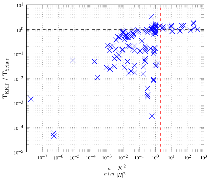
Figure 1. Runtime comparison of KKT and Schur complement methods when applying QPALM to the Maros Meszaros test set.

4.2. Computing the minimum eigenvalue

Finding the solution of a large symmetric eigenvalue problem has been the topic of a substantial body of research, and many methods exist. They are typically divided into two categories: direct methods, which find all eigenvalues, and iterative methods, which find some (or all) eigenvalues. The reader is referred to [28, §8] for a detailed overview of (the origin of) these methods. In our case, since we only need the minimum eigenvalue of $Q$, iterative methods seem more promising. Of these, the Locally Optimal Block Preconditioned Conjugate Gradient (LOBPCG) method, developed by Knyazev [35], demonstrated the best performance regarding robustness and speed of convergence in our tests. A dedicated implementation of LO(B)PCG to find only the minimum eigenvalue and its corresponding eigenvector was added in QPALM. This method iteratively minimizes the Rayleigh quotient $\frac{x^{\top}Qx}{x^{\top}x}$ in a Krylov subspace spanned by three vectors: the current eigenvector estimate $x^{k}$, the current residual $w^{k}=Qx^{k}-\lambda^{k}x^{k}$, and a conjugate gradient direction $p^{k}$. The details of the implementation in QPALM can be found in Algorithm 5. The computational cost of this algorithm per iteration is essentially a matrix-vector product and solving a 3-by-3 generalized eigenvalue system. The latter is performed in our code by finding the roots of a one-dimensional third-order polynomial and performing a Gaussian elimination of a 3-by-3 system. Note that Algorithm 5 is very similar to [35, Algorithm 4.1], aside from some scaling.

Algorithm 5

LO(B)PCG

5.1:   $x^{0}\in\mathbb{R}^{n},\varepsilon>0$ and $Q\in\operatorname{Sym}(\mathbb{R}^{n})$

5.2:   Lower bound on $\lambda^{*}=\lambda_{\rm min}(Q)$ and estimate of the corresponding eigenvector $x^{*}$ of $Q$

5.3:   Initialize $\lambda^{0}=\langle{}x^{0}{},{}Ax^{0}{}\rangle$, and $w^{0}=Qx^{0}-\lambda^{0}x^{0}$, and let $S=[x^{0},w^{0}]$

5.4:   Solve $S^{\top}QSy=\mu Sy$, set $\lambda^{1}=\min(\mu)$ and let $\tilde{y}$ denote the corresponding eigenvector

5.5:   $x^{1}=\tilde{y}_{1}x^{0}+\tilde{y}_{2}w^{0}$

5.6:   $p^{1}=\tilde{y}_{2}w^{0}$

5.7:   for  $k=1,2,\ldots$  do

5.8:       $w^{k}=Qx^{k}-\lambda^{k}x^{k}$

5.9:       if  $\|w^{k}\|_{2}\leq\varepsilon$  then

5.10:           Return $\lambda^{*}=\lambda^{k}-\|w^{k}\|_{2}$ and $x^{*}=x^{k}$     

5.11:       Let $S=[x^{k},w^{k},p^{k}]$

5.12:       Solve $S^{\top}QSy=\mu Sy$, set $\lambda^{k}=\min(\mu)$ and let $\tilde{y}$ denote the corresponding eigenvector

5.13:       $x^{k+1}=\tilde{y}_{1}x^{k}+\tilde{y}_{2}w^{k}+\tilde{y}_{3}p^{k}$

5.14:       $p^{k+1}=\tilde{y}_{2}w^{k}+\tilde{y}_{3}p^{k}$

5. Parameter selection

The little details can make or break the practical performance of an algorithm. This section discusses aspects that make QPALM more robust, such as preconditioning of the problem data, and the most important parameter settings. Some of these parameters and parameter update criteria have been tuned manually and some are computed automatically based on the problem data or current iterates. The last subsection also lays out in detail the termination criteria employed by QPALM.

5.1. Factorization updates

As mentioned in Section 4.1, in between Newton iterations we can update the factorization instead of having to refactorize from scratch. However, in practice, the factorization update routines will only be more efficient if the number of constraints entering and leaving the active set is relatively low. Hence, when the active set changes significantly, we want to recompute the factorization instead. After some experimental tuning, we decided on the following criterion to do an update:

$$|\mathcal{J}^{e}|+|\mathcal{J}^{l}|\leq\min(\texttt{max\_rank\_update},\texttt{ max\_rank\_update\_fraction}\cdot(n+m)),$$

with $\texttt{max\_rank\_update}=160$ an absolute limit and max_rank_update_fraction $=0.1$ a relative limit on the number of changing active constraints. Both of these parameters can also be set by the user.

5.2. Preconditioning

Most optimization solvers will perform a scaling of the problem in order to prevent too much ill conditioning. A standard idea in nonlinear optimization is to evaluate the objective and constraints and/or the norm of their gradients at a representative point and scale them respectively with their inverse, see for example [8, §12.5]. However, the quality of this scaling depends of course on the degree to which the initial point is representative for the iterates, and by extension the solution. Furthermore, since we are dealing with a QP, the constraints and objective are all determined by matrices. Therefore, it makes sense to equilibrate these matrices directly, as is done in OSQP for example [50, §5.1]. OSQP applies a modified Ruiz equilibration [48] to the KKT matrix. This equilibration routine iteratively scales the rows and columns in order to make their infinity norms go to 1. OSQP adds an additional step that scales the objective to take into account also the linear part $q$. We have found in our benchmarks, however, that instead of this scaling it is better to apply Ruiz equilibration to the constraints only, and to scale the objective by a single constant. Why exactly this is a better strategy is unknown to us, but we suspect that the constraints are more sensitive to the scaling, so it might be better to deal with them separately.

Algorithm 6

Ruiz equilibration [48]

6.1:   $A\in\mathbb{R}^{m\times n}$

6.2:   $D\in\mathbb{R}^{n},E\in\mathbb{R}^{m}$ and $\bar{A}=EAD$

6.3:   Initialize $\bar{A}=A$,  $D=I_{n}$,  $E=I_{m}$

6.4:   for  $k=1,\ldots,\texttt{scaling}$  do

6.5:       for  $i=1,\ldots,m$  do

6.6:           $\bar{E}_{ii}=\sqrt{\|\hat{A}_{i\cdot}\|_{\infty}}$     

6.7:       for  $j=1,\ldots,n$  do

6.8:           $\bar{D}_{jj}=\sqrt{\|\bar{A}_{\cdot j}\|_{\infty}}$     

6.9:       $\bar{A}={\bar{E}}^{-1}\bar{A}{\bar{D}}^{-1}$

6.10:       $D=D{\bar{D}}^{-1}$

6.11:       $E=E{\bar{E}}^{-1}$

In QPALM we apply Ruiz equilibration, outlined in Algorithm 6, to the constraint matrix $A$, yielding $\bar{A}=EAD$. The setting scaling denotes the number of scaling iterations which can be set by the user and defaults to 10. The objective is furthermore scaled by $c=\max(1.0,\|D(Qx^{0}+q)\|_{\infty})^{-1}$. In conclusion, we arrive at a scaled version of (1)

$$\operatorname*{minimize}_{\bar{x}\in\mathbb{R}^{n}}\tfrac{1}{2}\bar{x}^{\top}\bar{Q}\bar{x}+\bar{q}^{\top}\bar{x}\quad\operatorname{subject\ to}{}\bar{A}\bar{x}\in\bar{C},$$

with $\bar{x}=D^{-1}x$, $\bar{Q}=cDQD$, $\bar{q}=cDq$, $\bar{A}=EAD$, $\bar{C}={\mathopen{}\left\{z\in\mathbb{R}^{m}{}\mid{}\bar{\ell}\leq z\leq\bar{u}\right\}\mathclose{}}$, $\bar{\ell}=E\ell$ and $\bar{u}=Eu$. The dual variables in this problem are $\bar{y}=cE^{-1}y$. This is the problem that is actually solved in QPALM, although the termination criteria are unscaled, that is they apply to the original problem (1), see Section 5.4.

5.3. Penalty parameters

The choice of the penalty parameters, and the rules used to update them have been found to be a decisive factor in the performance of QPALM. In this section we discuss both the traditional penalty parameters arising in the augmented Lagrangian formulation $\Sigma_{\text{\sf{y}}}$, and the proximal penalty parameters $\Sigma_{\text{\sf{x}}}$.

5.3.1. Dual penalty parameters

The dual penalty parameters $\Sigma_{\text{\sf{y}}}$ play an integral role in slowly but surely enforcing feasibility over the iterations. Because the inner subproblems solved by QPALM are strongly convex, there is no theoretical requirement on the penalty parameters, other than the obvious one of them being positive. However, experience with augmented Lagrangian methods suggests that high values can inhibit convergence initially, as they then introduce ill conditioning in the problem, whereas high values near a solution are very useful to enforce feasibility. As such, these penalty parameters are typically increased during the solve routine depending on the constraint violations of the current iterate. A standard rule is to (only) increase the parameters when the respective constraint violations have not decreased sufficiently, see [43, §17.4]. Furthermore, an added rule in QPALM that is observed to work well is to increase the penalties proportional to their corresponding constraint violation. Hence, we employ the following strategy to find $\Sigma_{\text{\sf{y}},k+1}$ in 1.6 and 1.8 (based on scaled quantities):

$${\frac{(\Sigma_{\text{\sf{y}},k+1})_{ii}}{(\Sigma_{\text{\sf{y}},k})_{ii}}={\mathopen{}\left\{\begin{array}[]{l @{~~} >{\text{if~}}l<{\text{,}} }1.0\hfil\leavevmode\nobreak\ \leavevmode\nobreak\ &\leavevmode\nobreak\ }|(\bar{A}\bar{x}^{k+1}-\bar{z}^{k+1})_{i}|<\theta|(\bar{A}\bar{x}^{k}-\bar{z}^{k})_{i}|\\ \min{\mathopen{}\left[\frac{\sigma_{\max}}{(\Sigma_{\text{\sf{y}},k})_{ii}},\max{\mathopen{}\left(\mathbf{\Delta}\frac{|(\bar{A}\bar{x}^{k+1}-\bar{z}^{k+1})_{i}|}{\|\bar{A}\bar{x}^{k+1}-\bar{z}^{k+1}\|_{\infty}},1.0\right)\mathclose{}}\right]\mathclose{}}\hfil\leavevmode\nobreak\ \leavevmode\nobreak\ &\lx@intercol\text{otherwise.}\hfil\lx@intercol\end{array}\right.\mathclose{}}$$ (5.1)

The default parameters here are $\theta=0.25$, $\mathbf{\Delta}=100$, and $\sigma_{\max}=10^{9}$ and can all be set by the user. The usage of this rule, in particular letting the factor depend on the constraint violation itself, has been a crucial step in making the performance of QPALM more robust. In fact, it seems to us to be the key difference when compared to the corresponding penalty update in OSQP [50, §5.2], which uses the same factor for all the constraints and updates it only seldom based on the setup time and current runtime, in contrast to QPALM where each penalty is updated whenever the corresponding constraint violation has not sufficiently decreased (and is not already relatively small).

Note that in case only a few penalties are modified, the factorization of either $\widetilde{\mathcal{K}}$ or $H$ may be updated using low-rank update routines. In practice, we set the limit on the amount of changing penalties a bit lower as we expect an additional update to be required for the change in active constraints.

As with regards to an initial choice of penalty parameters, the formula proposed in [8, §12.4] was found to be effective after some tweaking of the parameters inside. As such we use the following rule to determine initial values of the penalties

$$(\Sigma_{\text{\sf{y}},0})_{ii}=\max{\mathopen{}\left[10^{-4},\min{\mathopen{}\left(\sigma_{\textrm{init}}\frac{\max(1.0,|\tfrac{1}{2}({\bar{x}}^{0})^{\top}\bar{Q}\bar{x}^{0}+\bar{q}^{\top}\bar{x}^{0}|)}{\max(1.0,\tfrac{1}{2}\|\bar{A}{\bar{x}}^{0}-\operatorname{\Pi}_{\bar{C}}(\bar{A}{\bar{x}}^{0})\|^{2})},10^{4}\right)\mathclose{}}\right]\mathclose{}},$$ (5.2)

with $\sigma_{\textrm{init}}$ a parameter with a default value of 20 and which can also be set by the user. Setting the initial penalty parameters to a high value can be very beneficial when provided with a good (feasible) initial guess, as therefore feasibility will not be lost. An investigation into this and warm-starting QPALM in general is a topic for future work.

5.3.2. Primal penalty parameters

The primal, or proximal, penalty parameters $\Sigma_{\text{\sf{x}}}$ serve to regularize the QP around the “current” point ${\hat{x}}^{k}$. An appropriate choice makes it so that the subproblems are strongly convex, as discussed before. In many problems, the user knows whether the QP at hand is convex or not. Therefore, QPALM allows the user to indicate which case is dealt with. If the user indicates the problem is (or might be) nonconvex, i.e. that $Q$ is not necessarily positive semidefinite, QPALM uses Algorithm 5 to obtain a tight lower bound $\lambda^{*}$ on the minimum eigenvalue. If this value is negative, we set $\forall i:\Sigma_{\text{\sf{x}},ii}=\frac{1}{|\lambda^{*}-10^{-6}|}$. Otherwise, or in case the user indicates the problem is convex, the default value is $\Sigma_{\text{\sf{x}},ii}^{-1}=10^{-7}$, a reasonably low value to not interfere with the convergence speed while guaranteeing that $H_{k}(x)$ or $\widetilde{\mathcal{K}}_{k}(x)$ is positive definite or quasidefinite respectively. This penalty has then a very similar effect as the Hessian regularization in OSQP [50], where the default is $10^{-6}I$. Furthermore, in the convex case, if the convergence is slow but the primal termination criterion (5.3b) is already satisfied, $\Sigma_{\text{\sf{x}},ii}^{-1}$ may be further decreased to $10^{-12}$ depending on an estimate of the (machine accuracy) errors that would be accumulated in $H_{k}(x)$. Finally, QPALM also allows the selection of an initial $\Sigma_{\text{\sf{x}},0,ii}=\gamma_{\rm init}$, and an update rule $\Sigma_{\text{\sf{x}},k+1,ii}=\min(\gamma_{\rm upd}\Sigma_{\text{\sf{x}},k+1,ii},\gamma_{\rm max})$, but this is not beneficial in practice. Not only does it not seem to speed up convergence on average, but every change in $\Sigma_{\text{\sf{x}}}$ also forces QPALM to refactorize the system.

5.4. Termination

This section discusses the termination criteria used in QPALM. Additionally to the criteria to determine a stationary point, we also discuss how to determine whether the problem is primal or dual infeasible.

5.4.1. Stationarity

Termination is based on the unscaled residuals, that is the residuals pertaining to the original problem (1). In QPALM, we allow for an absolute and a relative tolerance for both the primal and dual residual. As such, we terminate on an approximate stationary primal-dual pair $(\bar{x},\bar{y})$, with associated ${\bar{z}}^{k}{}={}\operatorname{\Pi}_{C}(\bar{A}{\bar{x}}+\Sigma_{\text{\sf{y}},k}^{-1}{\bar{y}})$, if

$$\tfrac{1}{c}\|D^{\scriptscriptstyle-1}(\bar{Q}{\bar{x}}{+}\bar{q}{+}\bar{A}^{\top}{\bar{y}})\|_{\scriptscriptstyle\infty}{}\leq{} \varepsilon_{\textrm{a}}{+}\tfrac{\varepsilon_{\textrm{r}}}{c}\max(\|D^{\scriptscriptstyle-1}\bar{Q}{\bar{x}}\|_{\scriptscriptstyle\infty},\|D^{\scriptscriptstyle-1}\bar{q}\|_{\scriptscriptstyle\infty},\|D^{\scriptscriptstyle-1}\bar{A}^{\top}{\bar{y}}\|_{\scriptscriptstyle\infty})$$ (5.3a)

$$\|E^{\scriptscriptstyle-1}(\bar{A}{\bar{x}}{-}{\bar{z}}^{k})\|_{\scriptscriptstyle\infty} {}\leq{}\varepsilon_{\textrm{a}}{+}\varepsilon_{\textrm{r}}\max(\|E^{\scriptscriptstyle-1}\bar{A}{\bar{x}}\|_{\scriptscriptstyle\infty},\|E^{\scriptscriptstyle-1}{\bar{z}}^{k}\|_{\scriptscriptstyle\infty}).$$ (5.3b)

Here, the tolerances $\varepsilon_{\textrm{a}}$ and $\varepsilon_{\textrm{r}}$ are by default $10^{-4}$ and can be chosen by the user. In the simulations of Section 7, these tolerances were always set to $10^{-6}$.

To determine termination of the subproblem in 1.3, following (2.15), the termination criterion

$$\textstyle\frac{1}{c}\|D^{\scriptscriptstyle-1}(\bar{Q}{\bar{x}}{+}\bar{q}{+}\Sigma_{\text{\sf{x}}}^{\scriptscriptstyle-1}({\bar{x}}-{\hat{\bar{x}}}^{k}){+}\bar{A}^{\top}{\bar{y}})\|_{\scriptscriptstyle\infty}{}\leq{}\delta_{\textrm{a},k}{+}\frac{\delta_{\textrm{r},k}}{c}\max(\|D^{\scriptscriptstyle-1}\bar{Q}{\bar{x}}\|_{\scriptscriptstyle\infty},\|D^{\scriptscriptstyle-1}\bar{q}\|_{\scriptscriptstyle\infty},\|D^{\scriptscriptstyle-1}\bar{A}^{\top}{\bar{y}}\|_{\scriptscriptstyle\infty})$$ (5.4)

is used. Here, the absolute and relative intermediate tolerances $\delta_{\textrm{a},k}$ and $\delta_{\textrm{r},k}$ start out from $\delta_{\textrm{a},0}$ and $\delta_{\textrm{r},0}$, which can be set by the user and default to $10^{0}$. In 1.9 they are updated using the following rule

$$\delta_{\textrm{a},k+1} {}={}\max(\rho\delta_{\textrm{a},k+1},\varepsilon_{\textrm{a}}),$$

$$\delta_{\textrm{r},k+1} {}={}\max(\rho\delta_{\textrm{r},k+1},\varepsilon_{\textrm{r}}),$$

with $\rho$ being the tolerance update factor, which can be set by the user and which defaults to $10^{-1}$. Note that, in theory, these intermediate tolerances should not be lower bounded but instead go to zero. In practice, this is however not possible due to machine accuracy errors. Furthermore, we have not perceived any inhibition on the convergence as a result of this lower bound. This makes sense as the inner subproblems are solved up to machine accuracy by the semismooth Newton method as soon as the correct active set is identified.

5.4.2. Infeasibility detection

Detecting infeasibility of a (convex) QP from the primal and dual iterates has been discussed in the literature [3]. The relevant criteria have also been implemented in QPALM, with a minor modification of the dual infeasibility criterion for a nonconvex QP. As such, we determine that the problem is primal infeasible if for a $\delta{\bar{y}}\neq 0$ the following two conditions hold

$$\|D^{\scriptscriptstyle-1}\bar{A}^{\top}\delta{\bar{y}}\|_{\scriptscriptstyle\infty} {}\leq{}\varepsilon_{\rm pinf}\|E\delta{\bar{y}}\|_{\scriptscriptstyle\infty},$$ (5.5a)

$$\bar{u}^{\top}[\delta{\bar{y}}]_{+}-\bar{l}^{\top}[-\delta{\bar{y}}]_{+} {}\leq-\varepsilon_{\rm pinf}\|E\delta{\bar{y}}\|_{\scriptscriptstyle\infty},$$ (5.5b)

with the certificate of primal infeasibility being $\frac{1}{c}E\delta{\bar{y}}$.

The problem is determined to be dual infeasible if for a $\delta{\bar{x}}\neq 0$

$${{{(E^{\scriptscriptstyle-1}\bar{A}\delta{\bar{x}})_{i}{\mathopen{}\left\{\begin{array}[]{l @{~~} >{\text{if~}}l<{\text{,}} }\in[-\varepsilon_{\rm dinf},\varepsilon_{\rm dinf}]\|D\delta{\bar{x}}\|_{\scriptscriptstyle\infty}\hfil\leavevmode\nobreak\ \leavevmode\nobreak\ &\leavevmode\nobreak\ }\bar{u}_{i},\bar{\ell}_{i}\in\mathbb{R}\\ \geq-\varepsilon_{\rm dinf}\|D\delta{\bar{x}}\|_{\scriptscriptstyle\infty}\hfil\leavevmode\nobreak\ \leavevmode\nobreak\ &\leavevmode\nobreak\ }\bar{u}_{i}=+\infty\\ \leq\varepsilon_{\rm dinf}\|D\delta{\bar{x}}\|_{\scriptscriptstyle\infty}\hfil\leavevmode\nobreak\ \leavevmode\nobreak\ &\leavevmode\nobreak\ }\bar{\ell}_{i}=-\infty\end{array}\right.\mathclose{}}$$ (5.6a)

holds for all $$i\in[1,m]$$, and either

$$\|D^{\scriptscriptstyle-1}\bar{Q}\delta{\bar{x}}\|_{\scriptscriptstyle\infty} {}\leq{}c\varepsilon_{\rm dinf}\|D\delta{\bar{x}}\|_{\scriptscriptstyle\infty},$$ (5.6b)

$$\bar{q}^{\top}\delta{\bar{x}} {}\leq-c\varepsilon_{\rm dinf}\|D\delta{\bar{x}}\|_{\scriptscriptstyle\infty}$$ (5.6c)

or

$$(\delta{\bar{x}})^{\top}\bar{Q}\delta{\bar{x}}\leq-c\varepsilon_{\rm dinf}^{2}\|\delta{\bar{x}}\|^{2}$$ (5.6d)

hold. Equations (5.6b) and (5.6c) express the original dual infeasibility for convex QPs, that is the conditions that $$\delta{\bar{x}} \delta{\bar{x}} -\infty \delta{\bar{x}}$$ is a direction of zero curvature and negative slope, whereas (5.6d) is added in the nonconvex case to determine whether the obtained is a direction of negative curvature. In the second case, the objective would go to quadratically along , and in the first case only linearly. Therefore, the square of the tolerance, assumed to be smaller than one, is used in (5.6d), so as to allow for earlier detection of this case. Note that we added minus signs in equations (5.5b) and (5.6c) in comparison to [3]. The reason for this is that the interpretation of our tolerance is different. In essence, [3] may declare some problems infeasible even though they are feasible. Our version prevents such false positives at the cost of requiring sufficient infeasibility and possibly a slower detection. We prefer this, however, over incorrectly terminating a problem, as many interesting problems in practice may be close to infeasible. When the tolerances are very close to zero, of course both versions converge to the same criterion.

The tolerances $\varepsilon_{\rm pinf}$ and $\varepsilon_{\rm dinf}$ can be set by the user and have a default value of $10^{-5}$.

6. The full QPALM algorithm

Algorithm 7 synopsizes all steps and details that make up the QPALM algorithm. Herein we set $\varepsilon_{{\rm a},0}=\delta_{{\rm a},0}$, $\varepsilon_{{\rm r},0}=\delta_{{\rm r},0}$. For brevity, the details on factorizations and updates necessary for 7.23, which have been discussed prior in Section 4.1, have been omitted here.

Algorithm 7

QPALM for the nonconvex problem (1)

7.1:   

Problem data: $Q\in\operatorname{Sym}(\mathbb{R}^{n})$;   $q\in\mathbb{R}^{n}$;   $A\in\mathbb{R}^{m\times n}$;   $\ell,u\in R^{m}$ with $\ell\leq u$;
$(x^{0},y^{0})\in\mathbb{R}^{n}\times\mathbb{R}^{m}$;   $\varepsilon_{\rm a},\varepsilon_{\rm r},\delta_{\rm a,0},\delta_{\rm r,0},\varepsilon_{\rm pinf},\varepsilon_{\rm dinf},{\varepsilon_{{\rm a},0},\varepsilon_{{\rm r},0},}\sigma_{\rm init},\sigma_{\rm max},\gamma>0$;   $\rho,\theta\in(0,1)$;
$\mathbf{\Delta}>1$;   $\texttt{scaling}\in\mathbb{N}$

7.2:   

Use Algorithm 6 to find $D$ and $E$, and let $c=\max(1.0,\|D(Qx^{0}+q)\|_{\infty})^{-1}$ Convert the data using

the scaling factors: ${\bar{x}}^{0}=D^{-1}x^{0}$, ${\bar{y}}^{0}=cE^{-1}y^{0}$, $\bar{Q}=cDQD$, $\bar{q}=cDq$, $\bar{A}=EAD$, $\bar{\ell}=E\ell$ and $\bar{u}=Eu$

7.3:   Initialize ${\hat{\bar{x}}}^{0}={\bar{x}}^{0}$, $\Sigma_{\text{\sf{y}},0}$ from (5.2) and $\delta\bar{x}=0$

7.4:^⋆   Compute $\lambda^{*}$ using Algorithm 5

7.5:^⋆   if  $\lambda^{*}<0$  then

7.6:^⋆       $\Sigma_{\text{\sf{x}},ii}=\frac{1}{|\lambda^{*}-10^{-6}|},\quad i=1,\ldots,n$

7.7:^⋆   else

7.8:       $\Sigma_{\text{\sf{x}},ii}=\gamma,\quad i=1,\ldots,n$

7.9:   for  $k=0,1,\ldots$  do

7.10:       Set ${\bar{x}}^{k,0}={\bar{x}}^{k}$

7.11:       for  $\nu=0,1,\ldots$  do

7.12:           ${\bar{z}}^{k,\nu}{}={}\operatorname{\Pi}_{\bar{C}}(\bar{A}{\bar{x}}^{k,\nu}+\Sigma_{\text{\sf{y}},k}^{-1}{\bar{y}}^{k})$

7.13:           $\delta{\bar{y}}=\Sigma_{\text{\sf{y}},k}(\bar{A}{\bar{x}}^{k,\nu}-{\bar{z}}^{k,\nu})$

7.14:           if  (5.3) is satisfied at $({\bar{x}}^{k,\nu},{\bar{y}}^{k}{}+\delta\bar{y})$  then

7.15:              return $({\bar{x}}^{k,\nu},{\bar{y}}^{k}+\delta{\bar{y}})$

7.16:           else if  (5.5) is satisfied at $\delta{\bar{y}}$  then

7.17:              return $c^{\scriptscriptstyle-1}E\delta{\bar{y}}$ as the certificate of primal infeasibility

7.18:           else if  (5.6) is satisfied at $\delta{\bar{x}}$  then

7.19:              return $D\delta{\bar{x}}$ as the certificate of dual infeasibility

7.20:           else if  (5.4) is satisfied at $({\bar{x}}^{k,\nu},{\bar{y}}^{k}+\delta{\bar{y}})$  then

7.21:              break

7.22:           else

7.23:              Find $d$ by solving either (3.3) or (3.4)

7.24:              Find $\tau$ using Algorithm 2

7.25:              $\delta{\bar{x}}=\tau d$

7.26:              ${\bar{x}}^{k,\nu+1}={\bar{x}}^{k,\nu}+\delta{\bar{x}}$              

7.27:       Set ${\bar{x}}^{k+1}={\bar{x}}^{k,\nu}$, ${\bar{z}}^{k+1}={\bar{z}}^{k,\nu}$ and ${\bar{y}}^{k+1}{}={}{\bar{y}}^{k}{}+{}\delta\bar{y}$

7.28:^⋆       if  $\|E^{\scriptscriptstyle-1}(\bar{A}{\bar{x}}^{k+1}-{\bar{z}}^{k+1})\|_{\scriptscriptstyle\infty}\leq\varepsilon_{{\rm a},k}+\varepsilon_{{\rm r},k}\max(\|E^{\scriptscriptstyle-1}\bar{A}{\bar{x}}^{k+1}\|_{\scriptscriptstyle\infty},\|E^{\scriptscriptstyle-1}{\bar{z}}^{k+1}\|_{\scriptscriptstyle\infty})$  then

7.29:           Update ${\hat{\bar{x}}}^{k+1}={\bar{x}}^{k+1}$

7.30:^⋆            $\varepsilon_{{\rm a},{k+1}}=\max(\rho\varepsilon_{{\rm a},{k}},\varepsilon_{\rm a})$ and $\varepsilon_{{\rm r},{k+1}}=\max(\rho\varepsilon_{{\rm r},{k}},\varepsilon_{\rm r})$

7.31:^⋆       else

7.32:^⋆            Set  ${\hat{\bar{x}}}^{k+1}={\hat{\bar{x}}}^{k}$, $\varepsilon_{{\rm a},{k+1}}=\varepsilon_{{\rm a},{k}}$ and $\varepsilon_{{\rm r},{k+1}}=\varepsilon_{{\rm r},{k}}$     

7.33:       Update $\Sigma_{\text{\sf{y}},k+1}$ according to (5.1)

7.34:       $\delta_{{\rm a},{k+1}}=\max(\rho\delta_{{\rm a},{k}},\varepsilon_{\rm a})$ and $\delta_{{\rm r},{k+1}}=\max(\rho\delta_{{\rm r},{k}},\varepsilon_{\rm r})$

It is interesting to note that QPALM algorithm presented here differs from its antecedent convex counterpart [33] only by the addition of the lines marked with a star “$\star$”, namely for the setting of $\Sigma_{\text{\sf{x}}}$ and the inner termination criteria. In the convex case, the starred lines are ignored and 7.8 and 7.29 will always activate. It is clear that the routines in QPALM require minimal changes when extended to nonconvex QPs. Furthermore, in numerical experience with nonconvex QPs the criterion of 7.28 seemed to be satisfied most of the time. Therefore, aside from the computation of a lower bound of the minimum eigenvalue of $Q$, QPALM behaves in a very similar manner for convex and for nonconvex QPs. Nevertheless, in practice convergence can be quite a bit slower due to the (necessary) heavy regularization induced by $\Sigma_{\text{\sf{x}}}$ if Q has a negative eigenvalue with a relatively large magnitude.

Table 1 lists the main user-settable parameters used in QPALM alongside their default values.

Name	Default value	Description
$\varepsilon_{\rm a}$	$10^{-4}$	Absolute tolerance on termination criteria
$\varepsilon_{\rm r}$	$10^{-4}$	Relative tolerance on termination criteria
$\delta_{{\rm a},0}$	$10^{0}$	Starting value of the absolute intermediate tolerance
$\delta_{{\rm r},0}$	$10^{0}$	Starting value of the relative intermediate tolerance
$\rho$	$10^{-1}$	Update factor for the intermediate tolerance
$\sigma_{\rm init}$	$20$	Used in the determination of the starting penalty parameters (cf. (5.2))
$\sigma_{\max}$	$10^{9}$	Cap on the penalty parameters
$\mathbf{\Delta}$	$100$	Factor used in updating the penalty parameters (cf. (5.1))
$\theta$	$0.25$	Used in determining which penalties to update (cf. (5.1))
$\gamma_{\rm init}$	$10^{7}$	Initial value of the proximal penalty parameter (convex case)
$\gamma_{\rm upd}$	$10$	Update factor for the proximal penalty parameter (convex case)
$\gamma_{\rm max}$	$10^{7}$	Cap on the proximal penalty parameter (convex case)
scaling	$10$	Number of Ruiz scaling iterations applied to $A$

Table 1. Main parameters used in QPALM and their default values.

7. Numerical Results

The performance of QPALM is benchmarked against other state-of-the-art solvers. For convex QPs, we chose the interior-point solver Gurobi (version 9.1.2) [32], the (parametric) active-set solver qpOASES (version 3.2.1) [24], and the operator splitting based solver OSQP (version 0.6.2) [50]. In addition, for the simulations on optimal control we added the tailored interior-point solver HPIPM (version 0.1.4) [25]. There are many other solvers available, some of which are tailored to certain problem classes, but the aforementioned ones provide a good sample of the main methods used for general convex QPs. For nonconvex QPs, however, no state-of-the-art open-source (local) optimization solver exists to our knowledge. Some open-source indefinite QP algorithms have been proposed, such as in [1]. However, their solver was found to run into numerical issues very often. The active-set solvers SQIC [27] and qpOASES [24] also work on indefinite QPs, although the former is not publicly available and the latter fails on most large-scale sparse problems in our benchmarks. Hence, we did not compare against a QP solver specifically, but rather against a state-of-the-art nonlinear optimization solver, IPOPT [55], when dealing with nonconvex QPs. All simulations were performed on a notebook with Intel(R) Core(TM) i7-7600U CPU @ 2.80GHz x 2 processor and 16 GB of memory. The convex problems are solved to a low and a medium-high accuracy value, with the termination tolerances $\varepsilon_{\rm a},\varepsilon_{\rm r}$ both set to $10^{-3}$ or $10^{-6}$ respectively for QPALM. In other solvers, the corresponding termination tolerances were similarly set to $10^{-3}$ or $10^{-6}$. This inevitably causes a bit of bloating in the presentation of the results, but it is the fairest way to compare the different algorithms, since the performance of certain solvers varies widely for different accuracies. For example, OSQP, being a first-order method, tends to find solutions at low accuracy quickly, but often fails to find solutions at high accuracy in a competitive time, as will be shown. The nonconvex problems were solved to an accuracy of $10^{-6}$ since we only compare against an interior-point method. Furthermore, for all solvers and all problems, the maximum number of iterations was set to infinity, and a time limit of 3600 seconds was specified.

7.1. Comparing runtimes

Comparing the performance of solvers on a benchmark test set is not straightforward, and the exact statistics used may influence the resulting conclusions greatly. In this paper, we will compare runtimes of different solvers on a set of QPs using two measures, the shifted geometric means (sgm) and the performance profiles. When dealing with specific problem classes, such as in Section 7.3.2 and Section 7.3.3, we will not use these statistics but instead make a simple plot of the runtime of the various solvers as a function of the problem dimension.

7.1.1. Shifted geometric means

Let $t_{\texttt{s,p}}$ denote the time required for solver s to solve problem p. Then the shifted geometric means $\bar{t}_{\texttt{s}}$ of the runtimes for solver s on problem set P is defined as

$$\bar{t}_{\texttt{s}}=\sqrt[\texttt{\small|P|}]{\prod_{\texttt{p}\in\texttt{P}}(t_{\texttt{s,p}}+\zeta)}-\zeta=e^{\frac{1}{\texttt{|P|}}\sum_{\texttt{p}\in\texttt{P}}\ln{(t_{\texttt{s,p}}+\zeta)}}-\zeta,$$

where the second formulation is used in practice to prevent overflow when computing the product. In this paper, runtimes are expressed in seconds, and a shift of $\zeta=1$ is used. Also note that we employ the convention that when a solver s fails to solve a problem p (within the time limit), the corresponding $t_{\texttt{s,p}}$ is set to the time limit for the computation of the sgm.

7.1.2. Performance profile

To compare the runtime performance in more detail, also performance profiles [21] are used. Such a performance profile plots the fraction of problems solved within a runtime of $f$ times the runtime of the fastest solver for that problem. Let S be the set of solvers tested, then

$$r_{\texttt{s,p}}=\frac{t_{\texttt{s,p}}}{\min_{\texttt{s}\in\texttt{S}}t_{\texttt{s,p}}},$$

denotes the performance ratio of solver s with respect to problem p. Note that by convention $r_{\texttt{s,p}}$ is set to $\infty$ when s fails to solve p (within the time limit). The fraction of problems $q_{\texttt{s}}(f)$ solved by s to within a multiple $f$ of the best runtime, is then given as

$$q_{\texttt{s}}(f)=\frac{1}{\texttt{|P|}}\sum_{\texttt{P}\ni\texttt{p}:r_{\texttt{s,p}}\leq f}1.$$

Performance profiles have been found to misrepresent the performance when more than two solvers were compared at the same time [29]. As such, we will construct only the performance profile of each other solver and QPALM, and abstain from comparing the other solvers amongst each other.

7.2. Nonconvex QPs

Nonconvex QPs arise in several application domains, such as in a reformulation of mixed integer quadratic programs and in the solution of partial differential equations. Furthermore, an indefinite QP has to be solved at every iteration of a sequential quadratic programming method applied to a nonconvex optimization problem. To have a broad range of sample QPs, we consider in this paper the set of nonconvex QPs included in the Cutest test framework [31]. LABEL:tab:cutest_long lists for each of those QPs the number of primal variables $n$ and the number of constraints $m$, excluding bound constraints. In addition, it lists a comparison of the runtime and final objective value for both QPALM and IPOPT. Given that both solvers only produce an (approximate) stationary point, and not necessarily the same, these results have been further analyzed to produce Table 3. Here, the problems have been divided according to whether both solvers converged to the same point or not, the criterion of which was set to a relative error on the primal solutions of $10^{-6}$.

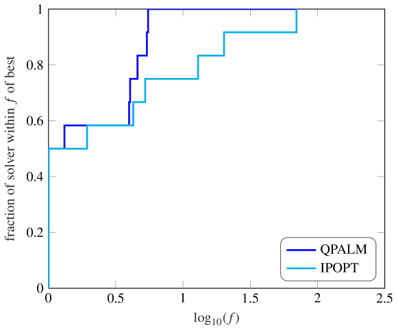
Figure 2. Performance profile for QPALM and IPOPT on the nonconvex QPs of the Cutest test set where both converged to the same approximate stationary point.

On the one hand, the runtimes of the problems where the same solution was found have been listed as shifted geometric means. It is clear that on average QPALM is competitive against IPOPT for these problems. These runtimes were further compared in the performance profile of Figure 2. This shows again that QPALM was competitive against IPOPT in runtimes. On the other hand, for the problems with different solutions, the objective value of the solution was compared and the number of times either QPALM or IPOPT had the lowest objective was counted. The resulting tally of 46 against 38 in favor of QPALM suggests there is no clear winner in this case. This was to be expected as both solvers report on the first stationary point obtained, and neither uses globalization or restarting procedures to obtain a better one.

The term dead points here refers to first-order stationary points which do not satisfy the second-order necessary condition that the reduced Hessian $Z^{\top}QZ$ be positive semidefinite, see [27, Result 2.2]. Here, $Z$ is the nullspace of $A_{\mathcal{J}\cdot}$, with $\mathcal{J}$ the set of active constraints, that is the constraints which hold as equality at the given point. It is clear from the table that both solvers find a few amount of dead points, although they do so on different problems.

Finally, also the failure rate was reported. It is clear that QPALM outperforms IPOPT by a small margin. Furthermore, for the six problems that QPALM failed to solve within the time limit, that is NCVXQP{1-3,7-9}, IPOPT also failed to solve in time. IPOPT reported two of the problems, A2NNDNIL and A5NNDNIL, as primal infeasible, whereas for these problems QPALM found a point satisfying the approximate stationary conditions. In fact, the problems are primal infeasible, and QPALM also reports this once slightly stricter termination tolerances are enforced. Hence, we consider both solvers to have succeeded for these two cases.

Table 2. Runtime and final objective value comparison for QPALM and IPOPT applied to the nonconvex QPs of the Cutest test set. Failure codes: PI = primal infeasible, DI = dual infeasible and F = time limit exceeded (or numerical issues).

			Runtime		Objective
Problem	n	m	QPALM	IPOPT	QPALM	IPOPT
A0ENDNDL	45006	15002	1.06e+01	1.92e+00	-1.71e-05	-1.84e-04
A0ENINDL	45006	15002	9.85e+00	1.83e+00	-4.61e-05	-1.84e-04
A0ENSNDL	45006	15002	4.68e+00	3.55e+01	-9.40e-06	-1.48e-04
A0ESDNDL	45006	15002	1.06e+01	2.66e+00	-5.47e-06	-1.84e-04
A0ESINDL	45006	15002	9.34e+00	2.03e+00	-2.21e-06	-1.84e-04
A0ESSNDL	45006	15002	4.42e+00	2.52e+01	-6.66e-06	-1.48e-04
A0NNDNDL	60012	20004	1.76e+02	7.88e+00	-3.22e-04	-1.84e-04
A0NNDNIL	60012	20004	3.55e+03	3.03e+01	-2.25e+00	-1.98e-04
A0NNDNSL	60012	20004	6.26e+01	2.56e+01	-4.81e-04	-2.15e-04
A0NNSNSL	60012	20004	1.87e+01	3.26e+01	-1.86e-04	-1.54e-04
A0NSDSDL	60012	20004	3.00e+01	5.83e+00	-2.29e-04	-1.84e-04
A0NSDSDS	6012	2004	1.49e+00	9.31e-01	-6.90e-06	-2.33e-04
A0NSDSIL	60012	20004	6.54e+02	3.00e+01	-1.77e-04	-1.97e-04
A0NSDSSL	60012	20004	3.11e+01	1.29e+01	-3.86e-06	-1.67e-04
A0NSSSSL	60012	20004	1.77e+01	3.02e+01	-5.65e-05	-1.49e-04
A2ENDNDL	45006	15002	2.63e+01	2.76e+00	-1.04e-06	-9.88e-04
A2ENINDL	45006	15002	2.53e+01	2.77e+00	-7.94e-07	-9.73e-04
A2ENSNDL	45006	15002	4.68e+00	4.11e+01	-9.99e-07	-2.10e-02
A2ESDNDL	45006	15002	2.75e+01	2.77e+00	-1.22e-06	-9.88e-04
A2ESINDL	45006	15002	2.52e+01	2.81e+00	-4.34e-07	-9.73e-04
A2ESSNDL	45006	15002	4.83e+00	3.91e+01	-2.03e-06	-2.22e-02
A2NNDNDL	60012	20004	1.43e+03	7.48e+00	-3.44e-04	-3.03e-04
A2NNDNIL	60012	20004	3.14e+01	PI	-5.11e+01	/
A2NNDNSL	60012	20004	3.48e+02	8.85e+01	-9.17e-07	-2.11e-04
A2NNSNSL	60012	20004	2.89e+01	3.17e+01	-3.59e-05	-1.46e-03
A2NSDSDL	60012	20004	5.15e+01	6.14e+00	-3.13e-06	-7.76e-04
A2NSDSIL	60012	20004	4.17e+01	4.20e+01	-5.95e-01	-1.57e+00
A2NSDSSL	60012	20004	4.08e+01	2.02e+01	-4.01e-06	-2.47e-02
A2NSSSSL	60012	20004	2.55e+01	2.94e+01	-8.81e-06	-4.69e-04
A5ENDNDL	45006	15002	4.97e+01	2.73e+00	-1.01e-06	-2.19e-03
A5ENINDL	45006	15002	5.38e+01	2.75e+00	-4.48e-07	-2.25e-03
A5ENSNDL	45006	15002	5.06e+00	3.72e+01	-4.15e-06	-5.12e-02
A5ESDNDL	45006	15002	5.25e+01	2.76e+00	-2.05e-06	-2.19e-03
A5ESINDL	45006	15002	5.14e+01	2.74e+00	-6.23e-07	-2.25e-03
A5ESSNDL	45006	15002	4.94e+00	3.68e+01	-1.86e-05	-5.12e-02
A5NNDNDL	60012	20004	2.02e+03	9.30e+00	-5.05e-04	-1.86e-03
A5NNDNIL	60012	20004	3.39e+01	PI	-1.02e+02	/
A5NNDNSL	60012	20004	2.27e+02	8.88e+01	-3.00e-06	-2.10e-04
A5NNSNSL	60012	20004	3.29e+01	4.22e+01	-3.63e-06	-1.38e-03
A5NSDSDL	60012	20004	9.73e+01	5.94e+00	-3.92e-06	-1.86e-03
A5NSDSDM	6012	2004	2.13e+00	8.69e-01	-1.14e-06	-2.33e-04
A5NSDSIL	60012	20004	3.76e+01	6.47e+01	-6.68e+00	-1.29e+00
A5NSDSSL	60012	20004	5.04e+01	1.97e+01	-1.11e-05	-1.00e-02
A5NSSNSM	6012	2004	1.52e+00	9.42e-01	-1.90e-06	-2.33e-04
A5NSSSSL	60012	20004	3.13e+01	7.58e+01	-4.78e-06	-2.45e-04
BIGGSC4	4	7	1.48e-04	5.41e-02	-2.45e+01	-2.45e+01
BLOCKQP1	10010	5001	1.64e-01	1.39e+01	-4.99e+03	-4.99e+03
BLOCKQP2	10010	5001	1.41e-01	1.83e+00	-4.99e+03	-4.99e+03
BLOCKQP3	10010	5001	2.69e+02	4.35e+02	-2.49e+03	-2.49e+03
BLOCKQP4	10010	5001	3.74e-01	1.96e+00	-2.50e+03	-2.50e+03
BLOCKQP5	10010	5001	2.56e+02	4.31e+02	-2.49e+03	-2.49e+03
BLOWEYA	4002	2002	1.86e+00	3.46e+03	-7.09e-06	-2.28e-02
BLOWEYB	4002	2002	3.76e-02	3.00e+03	-3.49e-05	-1.52e-02
BLOWEYC	4002	2002	6.64e-01	F	-2.92e-03	/
CLEUVEN3	1200	2973	6.85e+00	2.47e+01	-3.72e+05	-2.86e+05
CLEUVEN4	1200	2973	5.87e+02	5.74e+01	-2.84e+06	-2.86e+05
CLEUVEN5	1200	2973	6.42e+00	2.46e+01	-3.72e+05	-2.86e+05
CLEUVEN6	1200	3091	5.67e+00	2.25e+01	-2.21e+07	-2.21e+07
FERRISDC	2200	210	2.14e+00	2.58e+00	-1.02e-10	-2.13e-04
GOULDQP1	32	17	3.88e-03	7.84e-02	-3.49e+03	-3.49e+03
HATFLDH	4	7	1.25e-04	5.60e-02	-2.45e+01	-2.45e+01
HS44	4	6	6.92e-05	3.54e-02	-1.50e+01	-1.30e+01
HS44NEW	4	6	6.84e-05	4.78e-02	-1.50e+01	-1.30e+01
LEUVEN2	1530	2329	2.67e+00	1.96e+00	-1.41e+07	-1.41e+07
LEUVEN3	1200	2973	1.05e+03	2.45e+02	-1.38e+09	-1.99e+09
LEUVEN4	1200	2973	1.50e+01	4.84e+02	-4.78e+08	-1.83e+09
LEUVEN5	1200	2973	1.05e+03	2.62e+02	-1.38e+09	-1.99e+09
LEUVEN6	1200	3091	2.09e+03	1.05e+02	-1.17e+09	-1.19e+09
LEUVEN7	360	946	9.57e-02	4.14e-01	-6.95e+02	-6.95e+02
LINCONT	1257	419	PI	PI	/	/
MPC1	2550	3833	3.47e+00	6.73e+00	-2.33e+07	-2.33e+07
MPC10	1530	2351	4.82e+00	7.33e-01	-1.50e+07	-1.50e+07
MPC11	1530	2351	4.10e+00	8.09e-01	-1.50e+07	-1.50e+07
MPC12	1530	2351	4.32e+00	7.31e-01	-1.50e+07	-1.50e+07
MPC13	1530	2351	3.65e+00	7.39e-01	-1.50e+07	-1.50e+07
MPC14	1530	2351	3.54e+00	7.69e-01	-1.50e+07	-1.50e+07
MPC15	1530	2351	3.43e+00	7.72e-01	-1.50e+07	-1.50e+07
MPC16	1530	2351	2.92e+00	7.53e-01	-1.50e+07	-1.50e+07
MPC2	1530	2351	3.74e+00	6.67e-01	-1.50e+07	-1.50e+07
MPC3	1530	2351	2.99e+00	7.94e-01	-1.50e+07	-1.50e+07
MPC4	1530	2351	4.41e+00	6.74e-01	-1.50e+07	-1.50e+07
MPC5	1530	2351	4.12e+00	7.73e-01	-1.50e+07	-1.50e+07
MPC6	1530	2351	4.22e+00	7.71e-01	-1.50e+07	-1.50e+07
MPC7	1530	2351	4.17e+00	8.05e-01	-1.50e+07	-1.50e+07
MPC8	1530	2351	3.98e+00	7.60e-01	-1.50e+07	-1.50e+07
MPC9	1530	2351	4.47e+00	7.03e-01	-1.50e+07	-1.50e+07
NASH	72	24	PI	PI	/	/
NCVXQP1	10000	5000	F	F	/	/
NCVXQP2	10000	5000	F	F	/	/
NCVXQP3	10000	5000	F	F	/	/
NCVXQP4	10000	2500	1.06e+03	1.90e+03	-9.38e+09	-9.38e+09
NCVXQP5	10000	2500	1.52e+03	2.76e+03	-6.63e+09	-6.63e+09
NCVXQP6	10000	2500	2.49e+03	F	-3.40e+09	/
NCVXQP7	10000	7500	F	F	/	/
NCVXQP8	10000	7500	F	F	/	/
NCVXQP9	10000	7500	F	F	/	/
PORTSNQP	100000	2	3.80e+02	1.31e+00	-1.56e+00	-1.00e+00
QPNBAND	50000	25000	4.48e+00	3.41e+00	-2.50e+05	-2.50e+05
QPNBLEND	83	74	4.46e-03	5.49e-02	-9.14e-03	-9.13e-03
QPNBOEI1	384	351	2.09e-01	1.57e+00	-6.78e+06	-6.75e+06
QPNBOEI2	143	166	2.82e-02	8.54e-01	-1.37e+06	-1.37e+06
QPNSTAIR	467	356	6.88e-02	9.34e-01	-5.15e+06	-5.15e+06
SOSQP1	5000	2501	4.07e-02	1.74e-01	-4.24e-07	-1.03e-10
SOSQP2	5000	2501	9.44e-02	1.80e-01	-1.25e+03	-1.25e+03
STATIC3	434	96	DI	DI	/	/
STNQP1	8193	4095	1.51e+01	1.05e+03	-3.12e+05	-3.12e+05
STNQP2	8193	4095	2.99e+01	7.38e+00	-5.75e+05	-5.75e+05

	QPALM	IPOPT
Runtime (sgm)	4.0861	4.0761
Optimal	46	38
Dead points	7	4
Failure rate [%]	5.6075	7.4766

Table 3. Statistics of QPALM and IPOPT applied to the nonconvex QPs of the Cutest test set. The runtime reported is the mean over the 11 problems which converged to the same stationary point, whereas optimal denotes the number of times the solver found the stationary point with the lowest objective in problems where different stationary points were found. Dead points indicate points at which second-order necessary conditions are violated.

7.3. Convex QPs

Convex QPs arise in multiple well-known application domains, such as portfolio optimization and linear MPC. Solving such QPs has therefore been the subject of substantial research, and many methods exist. We compare QPALM against the interior-point solver Gurobi [32], the active-set solver qpOASES [24], and the operator splitting based solver OSQP [50]. First we compare all solvers on the Maros-Meszaros benchmark test set [40]. However, qpOASES is excluded in this comparison as it tends to fail on larger problems which are ubiquitous in this set. Then, the performance of all solvers is also compared for quadratic problems arising from the two aforementioned application domains, portfolio optimization and MPC. In the last case, we add the tailored interior-point solver HPIPM [25] to the benchmark.

7.3.1. Maros Meszaros

The Maros-Meszaros test set contains 138 convex quadratic programs, and is often used to benchmark convex QP solvers. Tables 4 and 5 list the shifted geometric mean of the runtime and failure rate of QPALM, OSQP and Gurobi applied to this set with termination tolerances respectively set to $10^{-3}$ and $10^{-6}$. A key aspect of QPALM that is demonstrated here is its robustness. The Maros-Meszaros set includes many large-scale and ill-conditioned QPs, and the fact that QPALM succeeds in solving all of them up to an accuracy of $10^{-6}$ within one hour is a clear indication that it is very robust with respect to the problem data. In runtime it is also faster on average than the other solvers. However, Gurobi is faster more often, as is shown in the performance profiles in Figures 3 and 4. The high shifted geometric mean runtime of Gurobi is mostly due to its relatively high failure rate. For a tolerance of $10^{-6}$, OSQP also has a high failure rate, and is slower than QPALM, both on average and in frequency. As a first-order method, in spite of employing a similar preconditioning routine to ours, it seems to still exhibit a lack of robustness with respect to ill conditioning and to somewhat stricter tolerance requirements. However, it clearly performs well on the set for a low tolerance of $10^{-3}$, as demonstrated in Tables 4 and 3. It only fails once and is faster than QPALM in almost 80% of the problems.

	QPALM	OSQP	Gurobi
Runtime (sgm)	0.5665	0.5943	1.4254
Failure rate [%]	0.0000	0.7246	9.4203

Table 4. Shifted geometric mean runtime and failure rate for QPALM, OSQP and Gurobi on the Maros Meszaros problem set with tolerance $10^{-3}$.

	QPALM	OSQP	Gurobi
Runtime (sgm)	0.8286	7.8153	1.4101
Failure rate [%]	0.0000	13.0435	9.4203

Table 5. Shifted geometric mean runtime and failure rate for QPALM, OSQP and Gurobi on the Maros Meszaros problem set with tolerance $10^{-6}$.

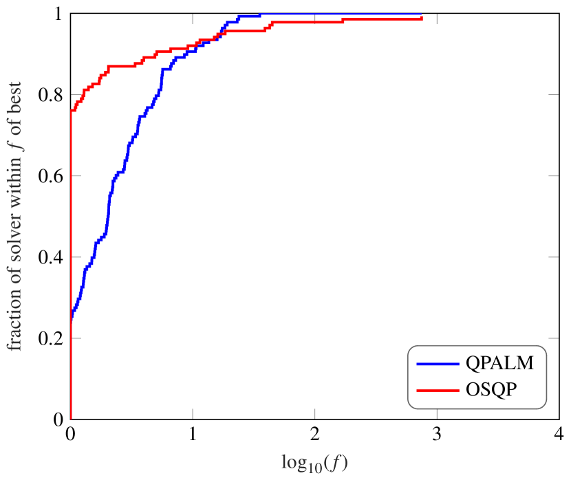
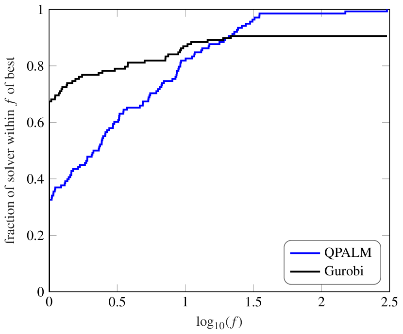
Figure 3. Performance profiles comparing QPALM with OSQP and Gurobi respectively on the Maros Meszaros problem set for a tolerance of $10^{-3}$.

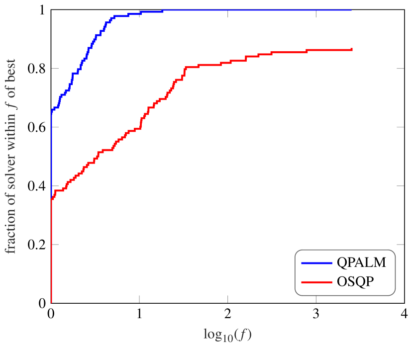
Figure 4. Performance profiles comparing QPALM with OSQP and Gurobi respectively on the Maros Meszaros problem set for a tolerance of $10^{-6}$.

7.3.2. Portfolio

In portfolio optimization, the goal is to select a portfolio of assets to invest in to maximize profit taking into account risk levels. Given a vector $x$ denoting the (relative) investment in each asset, the resulting quadratic program is the following

$$\operatorname*{minimize}_{x\in\mathbb{R}^{n}}\hskip 5.69046pt \beta x^{\top}\Sigma x-\mu^{\top}x$$

$$\operatorname{subject\ to}{}\hskip 5.69046pt x\geq 0,$$

$$\sum_{i=1}^{n}x_{i}=1,$$

with $\mu\in\mathbb{R}^{n}$ a vector of expected returns, $\Sigma\in\operatorname{Sym}(\mathbb{R}^{n})$ a covariance matrix representing the risk and $\beta>0$ a parameter to adjust the aversion to risk. Typically, $\Sigma=FF^{\top}+D$, with $F\in\mathbb{R}^{n\times r}$ a low rank matrix and $D\in\mathbb{R}^{n\times n}$ a diagonal matrix. In order not to form the matrix $\Sigma$, the following reformulated problem can be solved instead in $(x,y)$

$$\operatorname*{minimize}_{x\in\mathbb{R}^{n}}\hskip 5.69046pt \begin{bmatrix}x\\ y\end{bmatrix}^{\top}\begin{bmatrix}D&\\ &I_{r}\end{bmatrix}\begin{bmatrix}x\\ y\end{bmatrix}-\beta^{\scriptscriptstyle-1}\mu^{\top}x$$

$$\operatorname{subject\ to}{}\hskip 5.69046pt x\geq 0,$$

$$\sum_{i=1}^{n}x_{i}=1,$$

$$y=F^{\top}x.$$

We solved this problem for values of $n$ ranging from 100 to 1000, with $r=\lceil\frac{n}{10}\rceil$. We choose the elements of $\mu$ uniformly on $[0,1]$, the diagonal elements $D_{ii}$ uniformly on the interval $[0,\sqrt{r}]$, and the matrix $F$ has $50\%$ nonzeros drawn from $\mathcal{N}(0,1)$. For each value of $n$, we solve the problem for ten values of $\beta$ on a logarithmic scale between $10^{-2}$ and $10^{2}$ and compute the arithmetic mean of the runtimes. The runtimes of QPALM, OSQP, Gurobi and qpOASES solving these problems as such with tolerances $10^{-3}$ and $10^{-6}$ for different values of $n$ are shown in Figure 5. When warm-starting the problems from the solution of the problem with the previous $\beta$ value, Figure 6 is obtained. The structure of the portfolio optimization problem is quite specific: the Hessian of the objective is diagonal, and the only inequality constraints are bound constraints. It is clear from the figure that Gurobi exhibits the lowest runtimes for this type of problem, followed closely by QPALM and OSQP. The latter performs well especially for the small problems and has some robustness issues for larger ones. It seems qpOASES exhibits quite a high runtime when compared to the others. It is, however, the solver which benefits most from warm-starting in this scenario, as the runtime for warm-started problems is similar to the other solvers. Therefore, if very many values for $\beta$ were tested, the qpOASES curve would coincide with the others in Figure 6. QPALM and OSQP already exhibit low runtimes for this problem and do not benefit much from warm-starting here.

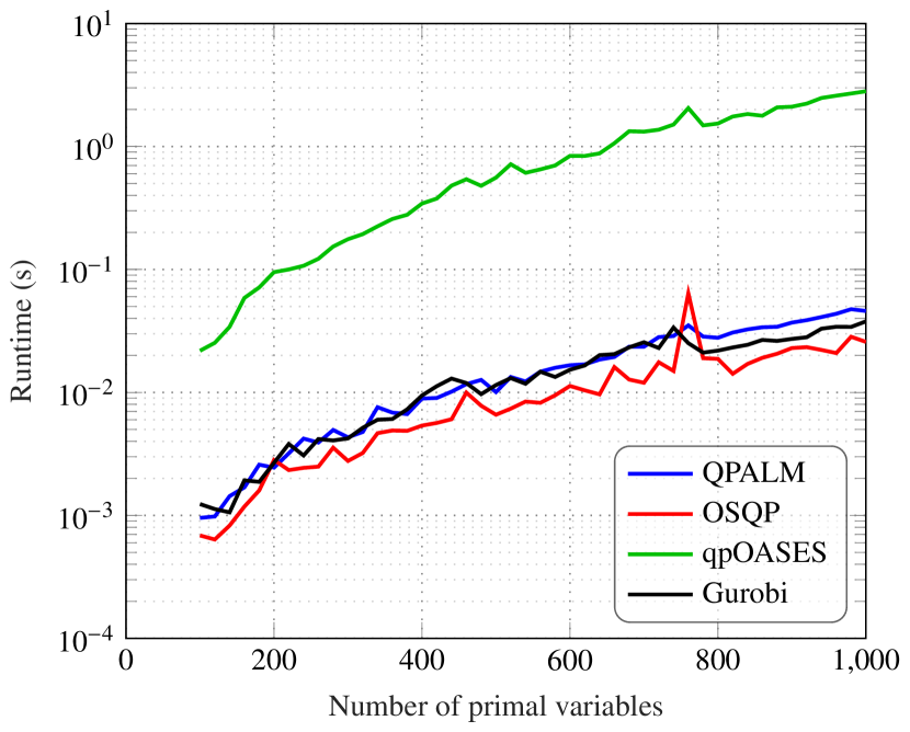
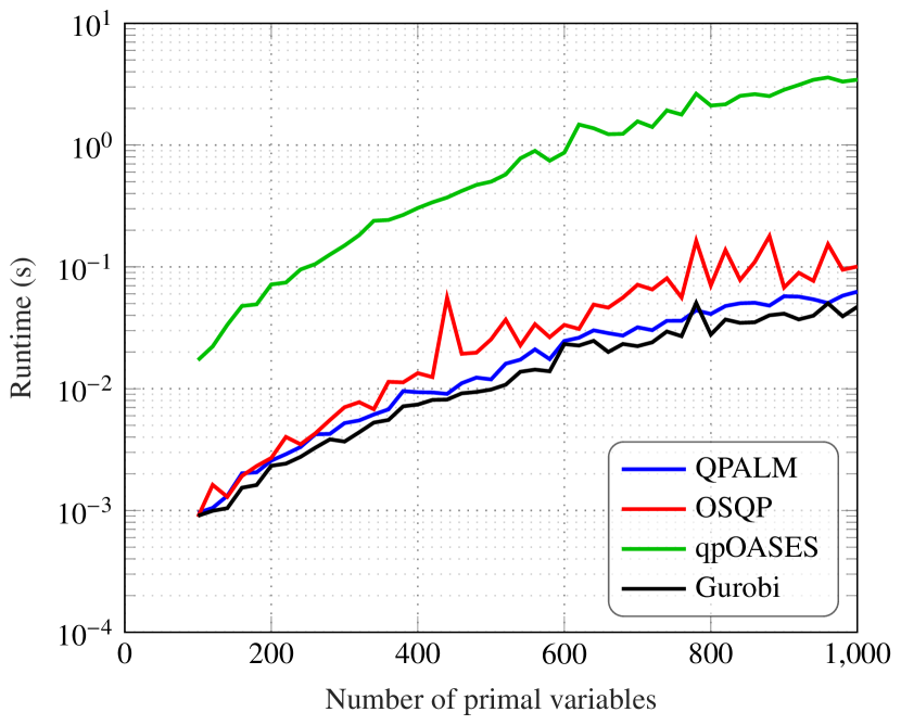
Figure 5. Runtimes of QPALM, OSQP, qpOASES and Gurobi when solving portfolio optimization problems of varying sizes. The tolerances are $10^{-3}$ and $10^{-6}$ left and right respectively.

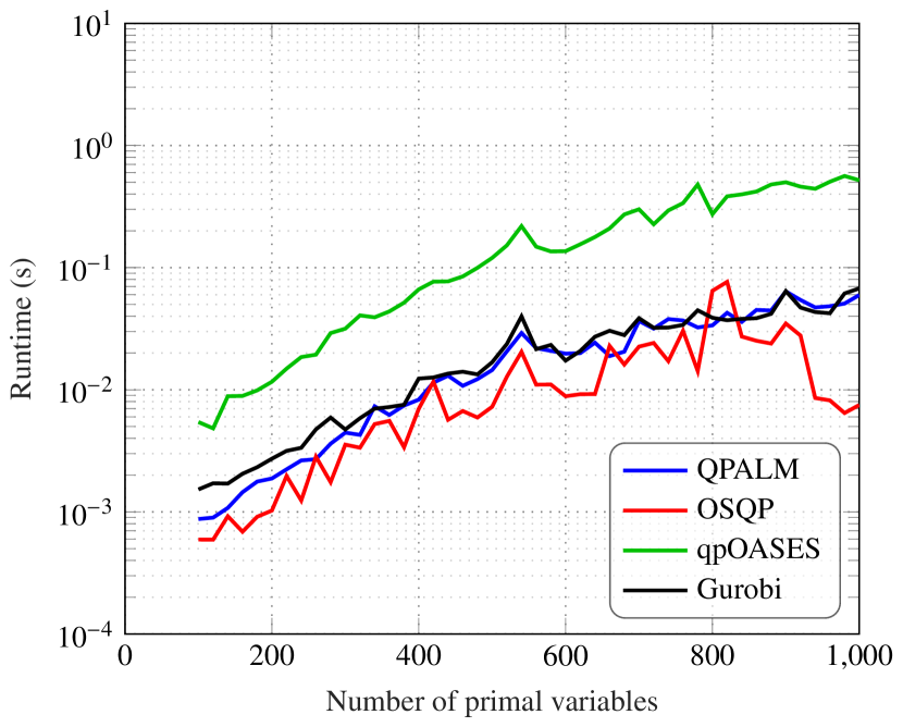
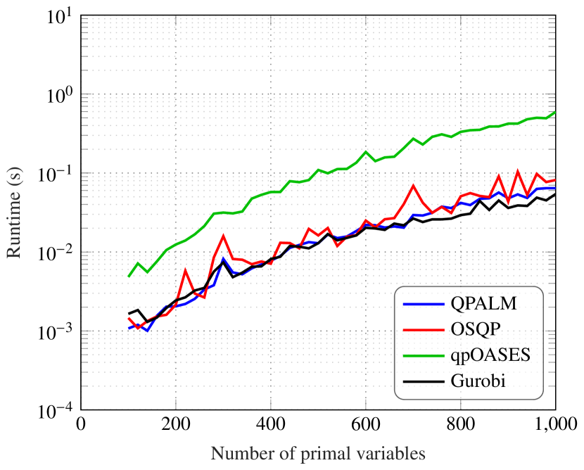
Figure 6. Runtimes of QPALM, OSQP, qpOASES and Gurobi when solving portfolio optimization problems of varying sizes and warm-starting in between different values of $\beta$. The tolerances are $10^{-3}$ and $10^{-6}$ left and right respectively.

7.3.3. MPC

In a model predictive control strategy, one solves an optimal control problem (OCP) at every sample time to determine the optimal control inputs that need to be applied to a system. The OCP considers a control horizon $N$, that is, it computes a series of $N$ inputs, of which only the first is applied to the system. Given a discrete linear system with $n_{x}$ states $x$ and $n_{u}$ inputs $u$, and its corresponding system dynamics in state-space form, $x_{k+1}=Ax_{k}+Bu_{k}$, the OCP we consider in this paper is one where we control the system from an initial state $\tilde{x}$ to the reference state at the origin, which can be formulated as

$$\operatorname*{minimize}_{z\in\mathbb{R}^{(N+1)n_{x}+Nn_{u}}}\hskip 5.69046pt x_{N}^{\top}Q_{N}x_{N}+\sum_{k=0}^{N-1}x_{k}^{\top}Qx_{k}+u_{k}^{\top}Ru_{k}$$

$$\operatorname{subject\ to}{}\hskip 5.69046pt x_{0}=\tilde{x},$$

$$x_{k+1}=Ax_{k}+Bu_{k},\quad k=0,\ldots,N-1,$$

$$x_{k}\in\mathcal{X},\quad k=0,\ldots,N-1,$$

$$x_{N}\in\mathcal{X}_{N},$$

$$u_{k}\in\mathcal{U},\quad k=0,\ldots,N-1.$$

Here, the decision variable is the collection of $N+1$ state samples and $N$ input samples, $z=(x_{0},u_{0},x_{1},\ldots,u_{N-1},x_{N})$. The stage and terminal state cost matrices are positive definite matrices, $Q,Q_{N}\in\operatorname{Sym}_{++}(\mathbb{R}^{n_{x}})$ and $R\in\operatorname{Sym}_{++}(\mathbb{R}^{n_{u}})$. $\mathcal{X}$, $\mathcal{X}_{N}$ and $\mathcal{U}$ represent polyhedral constraints on the states, terminal state and inputs respectively. In our example, we consider box constraints $\mathcal{X}=[-x_{b},x_{b}]$ and $\mathcal{U}=[-u_{b},u_{b}]$ and determine the terminal constraint as the maximum control invariant set of the system. Furthermore, the terminal cost is computed from the discrete-time algebraic Riccati equations.

We solved this problem for a system with 10 states and 5 inputs for different values of the time horizon. The state cost matrix is set as $Q=MM^{\top}$, with $M\in\mathbb{R}^{n_{x}\times n_{x}}$ consisting of $50\%$ nonzeros drawn from the normal distribution $\mathcal{N}(0,5)$. The input cost matrix is chosen to be a small diagonal matrix with $R_{ii}=0.01$. The system considered is slightly unstable, with the elements of $A$ drawn from $\mathcal{N}(0,2)$ and those of $B$ from $\mathcal{N}(0,1)$. The state and input limits $x_{b}$ and $u_{b}$ are drawn from $\mathcal{N}(10,2)$. Finally, the initial state is chosen such that it is possible but difficult to satisfy all the constraints, in order to represent a challenging MPC problem. The resulting runtimes of solving one such OCP for varying time horizons are shown in Figure 7 for tolerances $10^{-3}$ and $10^{-6}$. HPIPM performs best, as expected from a tailored solver, followed by Gurobi and QPALM. OSQP and qpOASES both have issues with robustness given the challenging nature of the problem, although the former performs well on small problems and the latter also exhibits fast convergence in some cases.

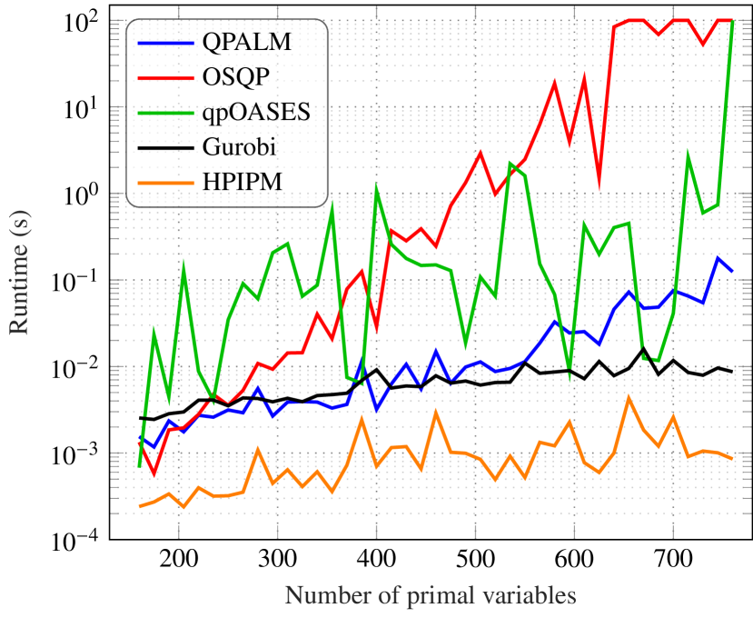
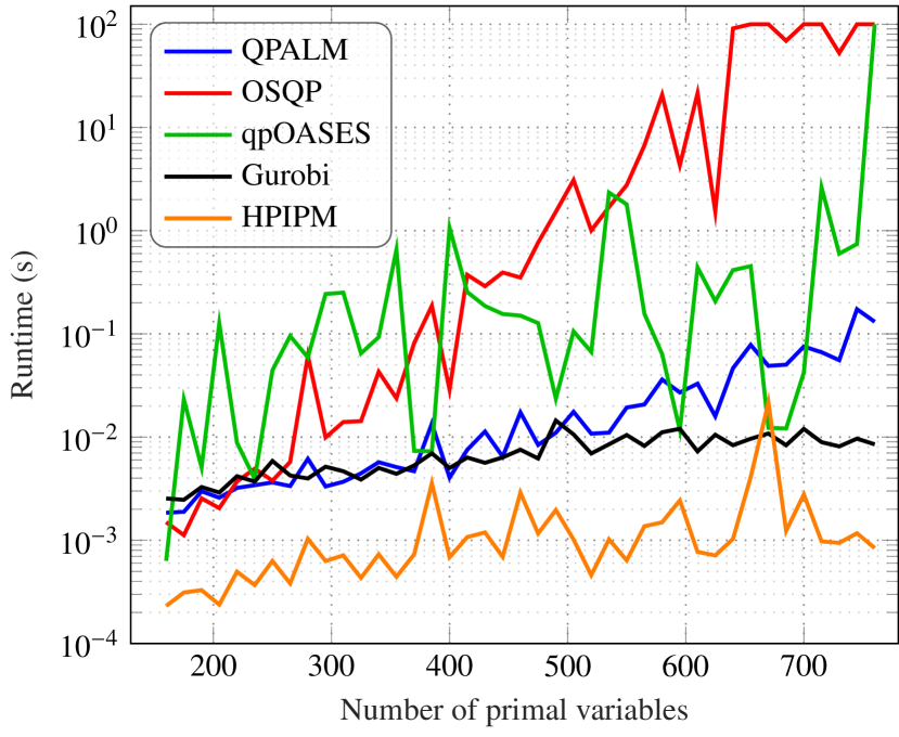
Figure 7. Runtimes of QPALM, OSQP, qpOASES, Gurobi and HPIPM when solving OCPs for varying time horizons. The tolerances are $10^{-3}$ and $10^{-6}$ left and right respectively.

An important aspect to consider when choosing a QP solver for MPC is the degree to which it can work with an initial guess. This is of great import due to the fact that subsequent OCPs are very similar. The solution of the previous OCP can therefore be shifted by one sample time and supplied as an initial guess. This procedure is also called warm-starting. Figure 8 shows the result of warm-starting subsequent OCP in this manner. Here, we solved 30 subsequent OCPs for a fixed time horizon of 30, corresponding to 460 primal variables. Furthermore, when computing the next initial state, we add a small disturbance drawn from the normal distribution $\mathcal{N}(0,0.01)$. It is clear that qpOASES, QPALM and OSQP all benefit greatly from this warm-starting. However, Gurobi, as is typical of an interior-point method, does not have this advantage. For this reason, interior-point methods are typically not considered as solvers for MPC problems. HPIPM, however, has incredibly low runtimes regardless, and so may be an excellent choice for optimal control problems.

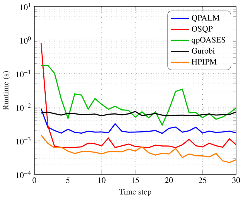
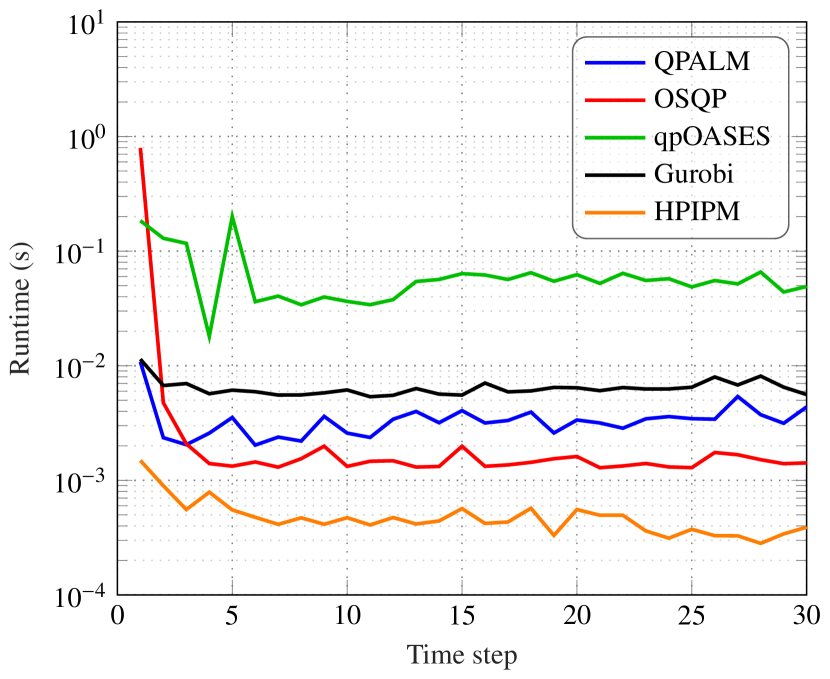
Figure 8. Runtimes of QPALM, OSQP, qpOASES, Gurobi and HPIPM when solving sequential OCPs in an MPC setting, with $N=30$. The tolerances are $10^{-3}$ and $10^{-6}$ left and right respectively.

8. Conclusion

This paper presented QPALM, a proximal augmented Lagrangian method for convex and nonconvex quadratic programming. On a theoretical level, it is shown that the sequence of inexact solutions of the proximal augmented Lagrangian, shown to be equivalent to inexact proximal point iterations, converges globally at an $R$-linear rate to a stationary point for the original problem when the proximal penalty ensures strong convexity of the inner subproblems. On a practical level, the implementation of QPALM is considered in great detail. The inner subproblems are solved using a direction obtained from a semismooth Newton method which relies on dedicated $LDL^{\top}$-factorization and factorization update routines, and on the optimal stepsize which can be efficiently computed as the zero of a monotone, piecewise affine function.

The QPALM algorithm is implemented in open-source C code, and parameter selection and update routines have all been worked out carefully. The resulting code is shown to strike a unique balance between robustness when faced with hard problems and efficiency when faced with easy problems. Given a time limit of one hour, QPALM can find an approximate stationary point or correctly identify infeasibility for 94.39% of the nonconvex QPs in the Cutest test set, whereas IPOPT does this only for 92.52%. Moreover, QPALM was able to solve all of the convex QPs in the Maros-Meszaros set up to a tolerance of $10^{-6}$, while Gurobi and OSQP exhibited a fail rate of 9.42% and 13.04%, respectively. These results are significant since the Cutest and Maros-Meszaros test-set contain some very large-scale and ill-conditioned QPs. Furthermore, QPALM benefits from warm-starting unlike interior-point methods.

A. Proofs of Theorem 2.2

 [Proof of Theorem 2.2]The proximal inequality

$$\varphi(x^{k+1}){}+{}\tfrac{1}{2}\|x^{k+1}-x^{k}-e^{k}\|_{\Sigma_{\text{\sf{x}}}^{-1}}^{2}{}\leq{}\varphi(x^{k}){}+{}\tfrac{1}{2}\|e^{k}\|_{\Sigma_{\text{\sf{x}}}^{-1}}^{2},$$

cf. (1.2), yields

$$\varphi(x^{k+1}){}+{}\tfrac{1}{4}\|x^{k+1}-x^{k}\|_{\Sigma_{\text{\sf{x}}}^{-1}}^{2}{}\leq{}\varphi(x^{k+1}){}+{}\tfrac{1}{2}\|x^{k+1}-x^{k}-e^{k}\|_{\Sigma_{\text{\sf{x}}}^{-1}}^{2}{}+{}\tfrac{1}{2}\|e^{k}\|_{\Sigma_{\text{\sf{x}}}^{-1}}^{2}{}\leq{}\varphi(x^{k}){}+{}\|e^{k}\|_{\Sigma_{\text{\sf{x}}}^{-1}}^{2},$$ (A.1)

proving assertions 2 and 4, and similarly 1 follows by invoking [45, Lem. 2.2.2]. Next, let $(x^{k})_{k\in K}$ be a subsequence converging to a point $x^{\star}$; then, it also holds that $(x^{k+1})_{k\in K}$ converges to $x^{\star}$ owing to assertion 2. From the proximal inequality (1.2) we have

$$\varphi(x^{k+1}){}+{}\tfrac{1}{2}\|x^{k+1}-x^{k}-e^{k}\|_{\Sigma_{\text{\sf{x}}}^{-1}}^{2}{}\leq{}\varphi(x^{\star}){}+{}\tfrac{1}{2}\|x^{\star}-x^{k}-e^{k}\|_{\Sigma_{\text{\sf{x}}}^{-1}}^{2},$$

so that passing to the limit for $K\ni k\to\infty$ we obtain that $\limsup_{k\in K}\varphi(x^{k+1})\leq\varphi(x^{\star})$. In fact, equality holds since $\varphi$ is lsc, hence from assertion 1 we conclude that $\varphi(x^{k+1})\to\varphi(x^{\star})$ as $k\to\infty$, and in turn from the arbitrarity of $x^{\star}$ it follows that $\varphi$ is constantly equal to this limit on the whole set of cluster points. To conclude the proof of assertion 3, observe that the inclusion $\Sigma_{\text{\sf{x}}}^{-1}(x^{k}+e^{k}-x^{k+1}){}\in{}\hat{\partial}\varphi(x^{k+1})$, cf. (1.3), implies that

$$\operatorname{dist}\bigl{(}0,\partial\varphi(x^{k+1})\bigr{)}{}\leq{}\operatorname{dist}\bigl{(}0,\hat{\partial}\varphi(x^{k+1})\bigr{)}{}\leq{}\|\Sigma_{\text{\sf{x}}}^{-1}\|{\mathopen{}\left(\|x^{k}-x^{k+1}\|{}+{}\|e^{k}\|\right)\mathclose{}},$$ (A.2)

and with limiting arguments (recall that $\lim_{k\in K}\varphi(x^{k})=\varphi(\lim_{k\in K}x^{k})$) the claimed stationarity of the cluster points is obtained.

References

- [1] Pierre-Antoine Absil and André L. Tits. Newton-KKT interior-point methods for indefinite quadratic programming. Computational Optimization and Applications, 36(1):5–41, 2007.
- [2] Patrick R. Amestoy, Timothy A. Davis, and Iain S. Duff. Algorithm 837: AMD, an approximate minimum degree ordering algorithm. ACM Transactions on Mathematical Software (TOMS), 30(3):381–388, 2004.
- [3] Goran Banjac, Paul Goulart, Bartolomeo Stellato, and Stephen Boyd. Infeasibility detection in the alternating direction method of multipliers for convex optimization. Journal of Optimization Theory and Applications, 183(2):490–519, 2019.
- [4] Michele Benzi, Gene H. Golub, and Jörg Liesen. Numerical solution of saddle point problems. Acta numerica, 14:1, 2005.
- [5] Dimitri P. Bertsekas. Convexification procedures and decomposition methods for nonconvex optimization problems. Journal of Optimization Theory and Applications, 29(2):169–197, Oct 1979.
- [6] Dimitri P. Bertsekas. Constrained optimization and Lagrange multiplier methods. Computer Science and Applied Mathematics, Boston: Academic Press, 1982, 1982.
- [7] Dimitri P. Bertsekas. Nonlinear Programming. Athena Scientific, 2016.
- [8] Ernesto G. Birgin and José Mario Martínez. Practical Augmented Lagrangian Methods for Constrained Optimization. Society for Industrial and Applied Mathematics, Philadelphia, PA, 2014.
- [9] Jérôme Bolte, Shoham Sabach, and Marc Teboulle. Nonconvex Lagrangian-based optimization: Monitoring schemes and global convergence. Mathematics of Operations Research, 43(4):1210–1232, 2018.
- [10] Radu Ioan Boţ and Dang-Khoa Nguyen. The proximal alternating direction method of multipliers in the nonconvex setting: Convergence analysis and rates. Mathematics of Operations Research, 45(2):682–712, 2020.
- [11] Samuel Burer and Dieter Vandenbussche. A finite branch-and-bound algorithm for nonconvex quadratic programming via semidefinite relaxations. Mathematical Programming, 113(2):259–282, 2008.
- [12] Jieqiu Chen and Samuel Burer. Globally solving nonconvex quadratic programming problems via completely positive programming. Mathematical Programming Computation, 4(1):33–52, 2012.
- [13] Yanqing Chen, Timothy A. Davis, William W. Hager, and Sivasankaran Rajamanickam. Algorithm 887: CHOLMOD, supernodal sparse Cholesky factorization and update/downdate. ACM Transactions on Mathematical Software (TOMS), 35(3):1–14, 2008.
- [14] Patrick L. Combettes and Teemu Pennanen. Proximal methods for cohypomonotone operators. SIAM journal on control and optimization, 43(2):731–742, 2004.
- [15] Richard W. Cottle, G.J. Habetler, and C.E. Lemke. On classes of copositive matrices. Linear Algebra and Its Applications, 3(3):295–310, 1970.
- [16] Timothy A. Davis. Algorithm 849: A concise sparse Cholesky factorization package. ACM Transactions on Mathematical Software (TOMS), 31(4):587–591, 2005.
- [17] Timothy A. Davis. Direct Methods for Sparse Linear Systems. Society for Industrial and Applied Mathematics, 2006.
- [18] Timothy A. Davis and William W. Hager. Modifying a sparse Cholesky factorization. SIAM Journal on Matrix Analysis and Applications, 20(3):606–627, 1999.
- [19] Timothy A. Davis and William W. Hager. Multiple-rank modifications of a sparse Cholesky factorization. SIAM Journal on Matrix Analysis and Applications, 22(4):997–1013, 2001.
- [20] Timothy A. Davis and William W. Hager. Row modifications of a sparse Cholesky factorization. SIAM Journal on Matrix Analysis and Applications, 26(3):621–639, 2005.
- [21] Elizabeth D. Dolan and Jorge J. Moré. Benchmarking optimization software with performance profiles. Mathematical programming, 91(2):201–213, 2002.
- [22] Asen L. Dontchev and R. Tyrrell Rockafellar. Implicit functions and solution mappings, volume 208. Springer, 2009.
- [23] Francisco Facchinei and Jong-Shi Pang. Finite-dimensional variational inequalities and complementarity problems, volume II. Springer, 2003.
- [24] Hans Joachim Ferreau, Christian Kirches, Andreas Potschka, Hans Georg Bock, and Moritz Diehl. qpOASES: A parametric active-set algorithm for quadratic programming. Mathematical Programming Computation, 6(4):327–363, 2014.
- [25] Gianluca Frison and Moritz Diehl. Hpipm: a high-performance quadratic programming framework for model predictive control. IFAC-PapersOnLine, 53(2):6563–6569, 2020.
- [26] E. Michael Gertz and Stephen J. Wright. Object-oriented software for quadratic programming. ACM Transactions on Mathematical Software (TOMS), 29(1):58–81, 2003.
- [27] Philip E. Gill and Elizabeth Wong. Methods for convex and general quadratic programming. Mathematical programming computation, 7(1):71–112, 2015.
- [28] Gene H. Golub and Charles F. Van Loan. Matrix Computations. Johns Hopkins Studies in the Mathematical Sciences. Johns Hopkins University Press, 2013.
- [29] Nicholas Gould and Jennifer Scott. A note on performance profiles for benchmarking software. ACM Transactions on Mathematical Software (TOMS), 43(2):1–5, 2016.
- [30] Nicholas I.M. Gould, Dominique Orban, and Philippe L. Toint. GALAHAD, a library of thread-safe fortran 90 packages for large-scale nonlinear optimization. ACM Transactions on Mathematical Software (TOMS), 29(4):353–372, 2003.
- [31] Nicholas I.M. Gould, Dominique Orban, and Philippe L. Toint. CUTEst: a constrained and unconstrained testing environment with safe threads for mathematical optimization. Computational Optimization and Applications, 60(3):545–557, 2015.
- [32] LLC Gurobi Optimization. Gurobi optimizer reference manual, 2018.
- [33] Ben Hermans, Andreas Themelis, and Panagiotis Patrinos. QPALM: A Newton-type proximal augmented Lagrangian method for quadratic programs. In 2019 IEEE 58th Conference on Decision and Control (CDC), pages 4325–4330, 2019.
- [34] Alfredo N. Iusem, Teemu Pennanen, and Benar F. Svaiter. Inexact variants of the proximal point algorithm without monotonicity. SIAM Journal on Optimization, 13(4):1080–1097, 2003.
- [35] Andrew V. Knyazev. Toward the optimal preconditioned eigensolver: Locally optimal block preconditioned conjugate gradient method. SIAM journal on scientific computing, 23(2):517–541, 2001.
- [36] Weiwei Kong, Jefferson G. Melo, and Renato D.C. Monteiro. Complexity of a quadratic penalty accelerated inexact proximal point method for solving linearly constrained nonconvex composite programs. SIAM Journal on Optimization, 29(4):2566–2593, 2019.
- [37] Guoyin Li and Ting Kei Pong. Global convergence of splitting methods for nonconvex composite optimization. SIAM Journal on Optimization, 25(4):2434–2460, 2015.
- [38] Qihang Lin, Runchao Ma, and Yangyang Xu. Inexact proximal-point penalty methods for non-convex optimization with non-convex constraints. arXiv preprint arXiv:1908.11518, 2019.
- [39] Zhi-Quan Luo and Paul Tseng. Error bounds and convergence analysis of feasible descent methods: a general approach. Annals of Operations Research, 46(1):157–178, 1993.
- [40] Istvan Maros and Csaba Mészáros. A repository of convex quadratic programming problems. Optimization Methods and Software, 11(1-4):671–681, 1999.
- [41] Csaba Mészáros. The BPMPD interior point solver for convex quadratic problems. Optimization Methods and Software, 11(1-4):431–449, 1999.
- [42] ApS MOSEK. Mosek optimization toolbox for matlab. User’s Guide and Reference Manual, Version, 9.2.22, 2019.
- [43] Jorge Nocedal and Stephen Wright. Numerical optimization. Springer Science & Business Media, 2006.
- [44] Panagiotis Patrinos and Haralambos Sarimveis. A new algorithm for solving convex parametric quadratic programs based on graphical derivatives of solution mappings. Automatica, 46(9):1405 – 1418, 2010.
- [45] Boris T. Polyak. Introduction to optimization. Inc., Publications Division, New York, 1, 1987.
- [46] R. Tyrrell Rockafellar. Augmented Lagrangians and applications of the proximal point algorithm in convex programming. Mathematics of Operations Research, 1(2):97–116, 1976.
- [47] R. Tyrrell Rockafellar and Roger J.B. Wets. Variational analysis, volume 317. Springer Science & Business Media, 2011.
- [48] Daniel Ruiz. A scaling algorithm to equilibrate both rows and columns norms in matrices. Technical report, Rutherford Appleton Laboratorie, 2001.
- [49] Hanif D. Sherali and Cihan H. Tuncbilek. A reformulation-convexification approach for solving nonconvex quadratic programming problems. Journal of Global Optimization, 7(1):1–31, 1995.
- [50] Bartolomeo Stellato, Goran Banjac, Paul Goulart, Alberto Bemporad, and Stephen Boyd. OSQP: An operator splitting solver for quadratic programs. Mathematical Programming Computation, 2020.
- [51] Tao Sun, Hao Jiang, Lizhi Cheng, and Wei Zhu. A convergence framework for inexact nonconvex and nonsmooth algorithms and its applications to several iterations. arXiv preprint arXiv:1709.04072, 2017.
- [52] Andreas Themelis, Masoud Ahookhosh, and Panagiotis Patrinos. On the acceleration of forward-backward splitting via an inexact Newton method. In R. Luke, H. Bauschke, and R. Burachik, editors, Splitting Algorithms, Modern Operator Theory, and Applications. Springer, 2019.
- [53] Andreas Themelis and Panagiotis Patrinos. Douglas–Rachford splitting and ADMM for nonconvex optimization: Tight convergence results. SIAM Journal on Optimization, 30(1):149–181, 2020.
- [54] Robert J. Vanderbei. Symmetric quasidefinite matrices. SIAM Journal on Optimization, 5(1):100–113, 1995.
- [55] Andreas Wächter and Lorenz T. Biegler. On the implementation of an interior-point filter line-search algorithm for large-scale nonlinear programming. Mathematical programming, 106(1):25–57, 2006.
- [56] Mihalis Yannakakis. Computing the minimum fill-in is NP-complete. SIAM Journal on Algebraic Discrete Methods, 2(1):77–79, 1981.
- [57] Yinyu Ye. On affine scaling algorithms for nonconvex quadratic programming. Mathematical Programming, 56(1-3):285–300, 1992.