Embedding Words in Non-Vector Space
with Unsupervised Graph Learning

Abstract

It has become a de-facto standard to represent words as elements of a vector space (word2vec, GloVe). While this approach is convenient, it is unnatural for language: words form a graph with a latent hierarchical structure, and this structure has to be revealed and encoded by word embeddings. We introduce GraphGlove: unsupervised graph word representations which are learned end-to-end. In our setting, each word is a node in a weighted graph and the distance between words is the shortest path distance between the corresponding nodes. We adopt a recent method learning a representation of data in the form of a differentiable weighted graph and use it to modify the GloVe training algorithm. We show that our graph-based representations substantially outperform vector-based methods on word similarity and analogy tasks. Our analysis reveals that the structure of the learned graphs is hierarchical and similar to that of WordNet, the geometry is highly non-trivial and contains subgraphs with different local topology.

1 Introduction

Effective word representations are a key component of machine learning models for most natural language processing tasks. The most popular approach to represent a word is to map it to a low-dimensional vector Mikolov et al. (2013b); Pennington et al. (2014); Bojanowski et al. (2017); Tifrea et al. (2019). Several algorithms can produce word embedding vectors with distances or dot products capturing semantic relationships between words; the vector representations can be useful for solving numerous NLP tasks such as word analogy Mikolov et al. (2013b), hypernymy detection Tifrea et al. (2019) or serving as features for supervised learning problems.

While representing words as vectors may be convenient, it is unnatural for language: words form a graph with a hierarchical structure Miller (1995) that has to be revealed and encoded by unsupervised learned word embeddings. A possible step towards this can be made by choosing a vector space more similar to the structure of the data: for example, a space with hyperbolic geometry Dhingra et al. (2018); Tifrea et al. (2019) instead of commonly used Euclidean Mikolov et al. (2013b); Pennington et al. (2014); Bojanowski et al. (2017) was shown beneficial for several tasks. However, learning data structure by choosing an appropriate vector space is likely to be neither optimal nor generalizable: Gu et al. (2018) argue that not only are different data better modelled by different spaces, but even for the same dataset the preferable type of space may vary across its parts. It means that the quality of the representations obtained from vector-based embeddings is determined by how well the geometry of the embedding space matches the structure of the data. Therefore, (1) any vector-based word embeddings inherit limitations imposed by the structure of the chosen vector space; (2) the vector space geometry greatly influences the properties of the learned embeddings; (3) these properties may be the ones of a space geometry and not the ones of a language.

In this work, we propose to embed words into a graph, which is more natural for language. In our setting, each word is a node in a weighted undirected graph and the distance between words is the shortest path distance between the corresponding nodes; note that any finite metric space can be represented in such a manner. We adopt a recently introduced method which learns a representation of data as a weighted graph Mazur et al. (2019) and use it to modify the GloVe algorithm for unsupervised word embeddings Pennington et al. (2014). The former enables simple end-to-end training by gradient descent, the latter — learning a graph in an unsupervised manner. Using the fixed training regime of GloVe, we vary the choice of a distance: the graph distance we introduced, as well as the ones defined by vector spaces: Euclidean Pennington et al. (2014) and hyperbolic Tifrea et al. (2019). This allows for a fair comparison of vector-based and graph-based approaches and analysis of limitations of vector spaces. In addition to improvements on a wide range of word similarity and analogy tasks, analysis of the structure of the learned graphs suggests that graph-based word representations can potentially be used as a tool for language analysis.

Our key contributions are as follows:

• we introduce GraphGlove — graph word embeddings;

• we show that GraphGlove substantially outperforms both Euclidean and Poincaré GloVe on word similarity and word analogy tasks;

• we analyze the learned graph structure and show that GraphGlove has hierarchical, similar to WordNet, structure and highly non-trivial geometry containing subgraphs with different local topology.

2 Graph Word Embeddings

For a vocabulary $\mathbf{V}=\{v_{0},v_{1},\dots,v_{n}\}$, we define graph word embeddings as an undirected weighted graph $G(V,E,w)$. In this graph,

• $V$ is a set of vertices corresponding to the vocabulary words;

• $E{=}\{e_{0},e_{1},\dots,e_{m}\}$ is a set of edges: $e_{i}{=}e(v_{src_{i}},v_{dst_{i}})$,   $v_{src_{i}}$, $v_{dst_{i}}\ \in V$;

• $w(e_{i})$ are non-negative edge weights.

When embedding words as vectors, the distance between words is defined as the distance between their vectors; the distance function is inherited from the chosen vector space (usually Euclidean). For graph word embeddings, the distance between words is defined as the shortest path distance between the corresponding nodes of the graph:

$$d_{G}(v_{i},v_{j})=\min\limits_{\pi\in\Pi_{G}(v_{i},v_{j})}\sum\limits_{e_{k}\in\pi}w(e_{k}),$$ (1)

where $\Pi_{G}(v_{i},v_{j})$ is the set of all paths from $v_{i}$ to $v_{j}$ over the edges of $G$.

To learn graph word embeddings, we use a recently introduced method for learning a representation of data in a form of a weighted graph Mazur et al. (2019) and modify the training procedure of GloVe Pennington et al. (2014) for learning unsupervised word embeddings. We give necessary background in Section 2.1 and introduce our method, GraphGlove, in Section 2.2.

2.1 Background

2.1.1 Learning Weighted Graphs

PRODIGE Mazur et al. (2019) is a method for learning a representation of data in a form of a weighted graph $G(V,E,w)$. The graph requires (i) inducing a set of edges $E$ from the data and (ii) learning edge weights. To induce a set of edges, the method starts from some sufficiently large initial set of edges and, along with edge weights, learns which of the edges can be removed from the graph. Formally, it learns $G(V,E,w,p)$, where in addition to a weight $w(e_{i})$, each edge $e_{i}$ has an associated Bernoulli random variable $b_{i}\sim Bern(p(e_{i}))$; this variable indicates whether an edge is present in $G$ or not. For simplicity, all random variables $b_{i}$ are assumed to be independent and the joint probability of all edges in the graph can be written as $p(G)=\prod_{i=0}^{m}p(e_{i})$. Since each edge is present in the graph with some probability, the distance is reformulated as the expected shortest path distance:

$$d(v_{i},v_{j})=\underset{G\sim p(G)}{\mathbb{E}}d_{G}(v_{i},v_{j})=$$

$$=\underset{G\sim p(G)}{\mathbb{E}}\ \ {\min\limits_{\pi\in\Pi_{G}(v_{i},v_{j})}}\sum_{e_{i}\in\pi}w(e_{i}),$$ (2)

where $d_{G}(v_{i},v_{j})$ is computed efficiently using Dijkstra’s algorithm. The probabilities $p(e_{i})$ are used only in training; at test time, edges with probabilities less than $0{.}5$ are removed, and the graph $G(V,E,w,p)$ can be treated as a deterministic graph $G(V,E,w)$.

Training.

Edge probabilities $p(e_{i})=p_{\theta}(e_{i})$ and weights $w(e_{i})=w_{\theta}(e_{i})$ are learned by minimizing the following training objective:

$$\vspace{-0.5ex}\mathcal{R(\theta)}=\underset{G\sim p(G)}{\mathbb{E}}\!\!\left[L(G,\theta)\right]{+}\lambda\cdot\frac{1}{|E|}\sum_{i=1}^{|E|}{p_{\theta}(e_{i})}.$$ (3)

Here $L(G,\theta)$ is a task-specific loss, and $\frac{1}{|E|}\sum_{i=1}^{|E|}{p_{\theta}(e_{i})}$ is the average probability of an edge being present. The second term is the $L_{0}$ regularizer on the number of edges, which penalizes edges for being present in the graph. Training with such regularization results in a graph where an edge becomes either redundant (with probability close to 0) or important (with probability close to 1).

To propagate gradients through the second term in (3), the authors use the log-derivative trick Glynn (1990) and Monte-Carlo estimate of the resulting gradient; when sampling, they also apply a heuristic to reduce variance. For more details on the optimization procedure, we refer the reader to the original paper Mazur et al. (2019).

Initialization.

An important detail is that training starts not from the set of all possible edges for a given set of vertices, but from a chosen subset; this subset is constructed using task-specific heuristics. The authors restrict training to a subset of edges to make it feasible for large datasets: while the number of all edges in a complete graph scales quadratically to the number of vertices, the initial subset can be constructed to scale linearly with the number of vertices.

2.1.2 GloVe

GloVe Pennington et al. (2014) is an unsupervised method which learns word representations directly from the global corpus statistics. Each word $v_{i}$ in the vocabulary $V$ is associated with two vectors $w_{i}$ and $\tilde{w}_{i}$; these vectors are learned by minimizing

$$\vspace{-1ex}\mathcal{J}\!\!=\!\!\sum\limits_{i,j=1}^{|V|}\!f(X_{i,j})(w_{i}^{T}\tilde{w}_{j}+b_{i}+\tilde{b}_{j}-\log X_{i,j})^{2}.$$ (4)

Here $X_{i,j}$ is the co-occurrence between words $v_{i}$ and $v_{j}$; $b_{i}$ and $\tilde{b}_{j}$ are trainable word biases, and $f(X_{i,j})$ is a weight function: $f(X_{i,j})=\min(1,[\frac{X_{i,j}}{x_{max}}]^{\alpha})$ with $x_{max}=100$ and $\alpha=3/4$.

The original GloVe learns embeddings in the Euclidean space; Poincaré GloVe Tifrea et al. (2019) adapts this training procedure to hyperbolic vector spaces. This is done by replacing $w_{i}^{T}\tilde{w}_{j}$ in formula (4) with $-h(d(w_{i},\tilde{w}_{j}))$, where $d(w_{i},\tilde{w}_{j})$ is a distance in the hyperbolic space, and $h$ is either $h(d)=d^{2}$ or $h(d)=\cosh^{2}(d)$ (see Table 1).

		“$\square$” in the loss term
		$f(X_{i,j})(\square+\!b_{i}\!+\!\tilde{b}_{j}\!-\!\log X_{i,j})^{2}$
Euclidean
		$w_{i}^{T}\tilde{w}_{j}$
Poincaré
	$d^{2}$	$-d^{2}(w_{i},\tilde{w}_{j})$
	$\cosh^{2}d$	$-\cosh^{2}\left(d(w_{i},\tilde{w}_{j})\right)$
Graph
	$d$	$-d_{G}(v_{i},v_{j})$
	$\langle\cdot,\cdot\rangle$	​​​​​​​​​ $\frac{1}{2}\left(-d_{G}^{2}(v_{i},v_{j})\!+\!d_{G}^{2}(v_{i},0)\!+\!d_{G}^{2}(v_{j},0)\right)$​​​

Table 1: Original GloVe loss and several extensions. For Poincaré GloVe, $d$ is distance in the hyperbolic space; for GraphGlove, $d$ is the shortest path distance.

2.2 Our Approach: GraphGlove

We learn graph word embeddings within the general framework described in Section 2.1.1. Therefore, it is sufficient to (i) define a task-specific loss $L(G,\theta)$ in formula (3), and (ii) specify the initial subset of edges.

2.2.1 Loss function

We adopt GloVe training procedure and learn edge weights and probabilities directly from the co-occurrence matrix $X$. We define $L(G,\theta)$ by modifying formula (4) for weighted graphs:

1. replace $w_{i}^{T}\tilde{w}_{j}$ with either graph distance or graph dot product as shown in Table 1 (see details below);

2. since we learn one representation for each word in contrast to two representations learned by GloVe, we set $\tilde{b}_{j}=b_{j}$.

Distance.

We want negative distance between nodes in a graph to reflect similarity between the corresponding words; therefore, it is natural to replace $w_{i}^{T}\tilde{w}_{j}$ with the graph distance. The resulting loss $L(G,\theta)$ is:

$$\sum_{i,j=1}^{|V|}\!\!f(X_{i,j})(-d_{G}(v_{i},v_{j})\!+\!b_{i}\!+\!b_{j}\!-\!\log X_{i,j})^{2}.\vspace{-1ex}$$ (5)

Dot product.

A more honest approach would be replacing dot product $w_{i}^{T}\tilde{w_{j}}$ with a “dot product” on a graph. To define dot product of nodes in a graph, we first express the dot product of vectors in terms of distances and norms. Let $w_{i}$, $w_{j}$ be vectors in a Euclidean vector space, then

$$|\!|w_{i}-w_{j}|\!|^{2}\! =\!|\!|w_{i}|\!|^{2}\!+\!|\!|w_{j}|\!|^{2}\!-\!2w_{i}^{T}w_{j},$$ (6)

$$w_{i}^{T}\!w_{j}\! =\!\frac{1}{2}\!\!\left(|\!|w_{i}|\!|^{2}\!+\!|\!|w_{j}|\!|^{2}\!\!-\!|\!|w_{i}\!-\!w_{j}|\!|^{2}\right)\!.$$ (7)

Now it is straightforward to define the dot product of nodes in our weighted graph:

$$\vspace{-1ex}\langle v_{i},v_{j}\rangle\!\!=\!\!\frac{1}{2}\!\left(d^{2}(v_{i},\!0)\!+\!d^{2}(v_{j},\!0)\!-\!d^{2}(v_{i},v_{j})\right)\!,$$ (8)

where $d(v_{i},v_{j})$ is the shortest path distance.

Note that dot product (8) contains distances to a zero element; thus in addition to word nodes, we also need to add an extra “zero” node in a graph. This is not necessary for the distance loss (5), but we add this node anyway to have a unified setting; a model can learn to use this node to build paths between other nodes.

All loss functions are summarized in Table 1.

2.2.2 Initialization

We initialize the set of edges by connecting each word with its $K$ nearest neighbors and $M$ randomly sampled words. The nearest neighbors are computed as closest words in the Euclidean GloVe embedding space, random words are sampled uniformly from the vocabulary.

We initialize biases $b_{i}$ from the normal distribution $\mathcal{N}(0,0{.}01)$, edge weights by the cosine similarity between the corresponding GloVe vectors, and edge probabilities with $0{.}9$.

3 Experimental Setup

3.1 Baselines

Our baselines are Euclidean GloVe Pennington et al. (2014) and Poincaré GloVe Tifrea et al. (2019); for both, we use the original implementation with recommended hyperparameters. We chose these models to enable a comparison of our graph-based method and two different vector-based approaches within the same training scheme.

3.2 Corpora and Preprocessing

We train all embeddings on Wikipedia 2017 corpus. To improve the reproducibility of our results, we (1) use a standard publicly available Wikipedia snapshot from gensim-data, (2) process the data with standard GenSim Wikipedia tokenizer. Also, we release preprocessing scripts and the resulting corpora as a part of the supplementary code.

3.3 Setup

We compare embeddings with the same vocabulary and number of parameters per token. For vector-based embeddings, the number of parameters equals vector dimensionality. For GraphGlove, we compute number of parameters per token as proposed by Mazur et al. (2019): ($|V|+2\cdot|E|)/|V|$. To obtain the desired number of parameters in GraphGlove, we initialize it with several times more parameters and train it with $L_{0}$ regularizer until enough edges are dropped (see Section 2.2).

We consider two vocabulary sizes: 50k and 200k. For 50k vocabulary, the models are trained with either 20 or 100 parameters per token; for 200k vocabulary — with 20 parameters per token. For initialization of GraphGlove with 20 parameters per token we set $K=64$, $M=10$; for a model with 100 parameters per token, $K=480$, $M=32$.

In preliminary experiments, we discovered that increasing both $K$ and $M$ leads to better final representations at a cost of slower convergence; decreasing the initial graph size results in lower quality and faster training. However, starting with no random edges (i.e. $M=0$) also slows convergence down.

3.4 Training

Similarly to vectorial embeddings, GraphGlove learns to minimize the objective (either distance or dot product) by minibatch gradient descent. However, doing so efficiently requires a special graph-aware batching strategy. Namely, a batch has to contain only a small number of rows with potentially thousands of columns per row. This strategy takes advantage of the Dijkstra algorithm: a single run of the algorithm can find the shortest paths between a single source and multiple targets. Formally, one training step is as follows:

1. we choose $b=64$ unique “anchor” words;

2. sample up to $n=10^{4}$ words that co-occur with each of $b$ “anchors”;

3. multiply the objective by importance sampling weights to compensate for non-uniform sampling strategy.

This way, a single training iteration with $b\cdot n$ batch size requires only $O(b)$ runs of Dijkstra algorithm.

After computing the gradients for a minibatch, we update GraphGlove parameters using Adam Kingma and Ba (2014) with learning rate $\alpha{=}0.01$ and standard hyperparameters ($\beta_{1}{=}0.9,\beta_{2}{=}0.999$).

It took us less than 3.5 hours on a 32-core CPU to train GraphGlove on 50k tokens until convergence. This is approximately 3 times longer than Euclidean GloVe in the same setting.

4 Experiments

In the main text, we report results for 50k vocabulary with 20 parameters per token. Results for other settings, as well as the standard deviations, can be found in the supplementary material.

4.1 Word Similarity

To measure similarity of a pair of words, we use cosine distance for Euclidean GloVe, the hyperbolic distance for Poincaré GloVe and the shortest path distance for GraphGlove. In the main experiments, we exclude pairs with out-of-vocabulary (OOV) words. In the supplementary material, we also provide results with inferred distances for OOV words.

We evaluate word similarity on standard benchmarks: WS353, SCWS, RareWord, SimLex and SimVerb. These benchmarks evaluate Spearman rank correlation of human-annotated similarities between pairs of words and model predictions. Table 2 shows that GraphGlove outperforms vector-based embeddings by a large margin.

		​​​​​​​SCWS	WS353	RW	SL	SV
Euclidean
		54.0	46.1	31.4	20.1	08.7
Poincaré
	$d^{2}$	45.5	41.0	33.7	23.0	10.9
	$\cosh^{2}d$	53.5	51.3	36.1	23.5	11.6
Graph
	$d$	56.2	56.7	37.2	30.4	10.3
	$\langle\cdot,\cdot\rangle$	53.4	58.6	35.5	30.0	14.4

Table 2: Spearman rank correlation on word similarity tasks; best is bold, second best is underlined. 50k vocabulary, 20 parameters per token. Results for other setups can be found in the supplementary material.

4.2 Word Analogy

Analogy prediction is a standard method for evaluation of word embeddings. This task typically contains tuples of 4 words: $(a,a^{*},b,b^{*})$ such that $a$ is to $a^{*}$ as $b$ is to $b^{*}$. The model is tasked to predict $b^{*}$ given the other three words: for example, “$a=Athens$ is to $a^{*}=Greece$ as $b=Berlin$ is to $b^{*}=\underline{\hskip 28.45274pt}(Germany)$”. Models are compared based on accuracy of their predictions across all tuples in the benchmark.

Datasets.

We use two test sets: standard benchmarks Mikolov et al. (2013b, c) and the Bigger Analogy Test Set (BATS) Gladkova et al. (2016).

The standard benchmarks contain Google analogy Mikolov et al. (2013a) and MSR Mikolov et al. (2013c) test sets. MSR test set contains only morphological category; Google test set contains 9 morphological and 5 semantic categories, with 20 –70 unique word pairs per category combined in all possible ways to yield 8,869 semantic and 10,675 syntactic questions. Unfortunately, these test sets are not balanced in terms of linguistic relations, which may lead to overestimation of analogical reasoning abilities as a whole Gladkova et al. (2016).

The Bigger Analogy Test Set (BATS) Gladkova et al. (2016) contains 40 linguistic relations, each represented with 50 unique word pairs, making up 99,200 questions in total. In contrast to the standard benchmarks, BATS is balanced across four groups: inflectional and derivational morphology, and lexicographic and encyclopedic semantics.

Evaluation.

Euclidean GloVe solves analogies by maximizing the 3CosAdd score:

$$b^{*}{=}\!\!\underset{\hat{b}\in V\setminus\{a^{*},a,b\}}{\arg\!\max}\!\!\left({\cos(\hat{b},a^{*}){-}\cos(\hat{b},a){+}\cos(\hat{b},b)}\right).$$

We adapt this for GraphGlove by substituting $\cos(x,y)$ with a graph-based similarity function. As a simple heuristic, we define the similarity between two words as the correlation of vectors consisting of distances to all words in the vocabulary:

$$\vec{d}_{G}(x)=(d_{G}(x,v_{0}),...,d_{G}(x,v_{N}))$$

$$\text{sim}_{G}(x,y):=\text{corr}(\vec{d}_{G}(x),\vec{d}_{G}(y))$$

This function behaves similarly to the cosine similarity: its values are from -1 to 1, with unrelated words having similarity close to 0 and semantically close words having similarity close to 1. Another alluring property of $\text{sim}_{G}(x,y)$ is efficient computation: we can get full distance vector $\vec{d}_{G}(x)$ with a single pass of Dijkstra’s algorithm.

We use $\text{sim}_{G}(x,y)$ to solve the analogy task in GraphGlove:

$$b^{*}{=}\!\!\underset{\hat{b}\in V\setminus\{a^{*},a,b\}}{\!\arg\!\max}\!\!\!\left(\!{\text{sim}(\hat{b},a^{*})}{-}\text{sim}(\hat{b},a){+}\text{sim}(\hat{b},b)\right).$$

For details on how Poincaré GloVe solves the analogy problem, we refer the reader to the original paper Tifrea et al. (2019).

Results.

GraphGlove shows substantial improvements over vector-based baselines (Tables 3 and 4). Note that for Poincaré GloVe, the best-performing loss functions for the two tasks are different ($\cosh^{2}d$ for similarity and $d^{2}$ for analogy), and there is no setting where Poincaré GloVe outperforms Euclidean Glove on both tasks. While for GraphGlove best-performing loss functions also vary across tasks, GraphGlove with the dot product loss outperforms all vector-based embeddings on 10 out of 13 benchmarks (both analogy and similarity). This shows that when removing limitations imposed by the geometry of a vector space, embeddings can better reflect the structure of the data. We further confirm this by analyzing the properties of the learned graphs in Section 5.

		Sem.	Syn.	Full	MSR
Euclidean
		30.8	20.9	25.2	15.5
Poincaré
	$d^{2}$	31.5	20.3	25.4	19.7
	$\cosh^{2}d$	30.5	16.9	23.1	18.1
Graph
	$d$	31.3	20.5	25.4	16.1
	$\langle\cdot,\cdot\rangle$	33.0	24.2	28.2	21.7

Table 3: Accuracy word analogy tasks; best is bold, second best is underlined. 50k vocabulary, 20 parameters per token. Results for other setups can be found in the supplementary material. (Sem., Syn. and Full are Google benchmarks Mikolov et al. (2013a)).

		​​​​​​​Inf.	Der.	Lex.	Enc.
Euclidean
		14.3	2.1	18.3	3.7
Poincaré
	$d^{2}$	14.8	2.3	18.9	4.3
	$\cosh^{2}d$	15.7	2.4	19.2	4.4
Graph
	$d$	15.9	2.3	19.3	4.6
	$\langle\cdot,\cdot\rangle$	16.9	2.2	20.6	5.4

Table 4: Spearman rank correlation on BATS word analogy dataset; best is bold, second best is underlined. 50k vocabulary, 20 parameters per token.

5 Learned Graph Structure

In this section, we analyze the graph structure learned by our method and reveal its differences from the structure of vector-based embeddings.

We compare graph $G_{G}$ learned by GraphGlove ($d$) with graphs $G_{E}$ and $G_{P}$ induced from Euclidean and Poincaré ($\cosh^{2}d$) embeddings respectively. For vector embeddings, we consider two methods of graph construction:

1. thr – connect two nodes if they are closer than some threshold $\tau$,

2. knn – connect each node to its $K$ nearest neighbors and combine multiple edges.

The values $\tau$ and $K$ are chosen to have similar edge density for all graphs.

We find that in contrast to the graphs induced from vector embeddings:

• in GraphGlove frequent and generic words are highly interconnected;

• GraphGlove has hierarchical, similar to WordNet, structure;

• GraphGlove has non-trivial geometry containing subgraphs with different local topology.

5.1 Important words

Here we identify which words correspond to “central” (or important) nodes in different graphs; we consider several notions of node centrality frequently used in graph theory. Note that in this section, by word importance we mean graph-based properties of nodes (e.g. the number of neighbors), and not semantic importance (e.g., high importance for content words and low for function words).

Degree centrality.

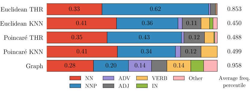
Figure 1: Top-200 words, the degree centrality. POS distribution and the average frequency percentile.

The simplest measure of node importance is its degree. For the top 200 nodes with the highest degree, we show the distribution of parts of speech and the average frequency percentile (higher means more frequent words). Figure 1 shows that for all vector-based graphs, the top contains a significant fraction of proper nouns and nouns. For $G_{G}$, distribution of parts of speech is more uniform and the words are more frequent. We provide the top words and all subsequent importance measures in the supplementary material.

Eigenvector centrality.

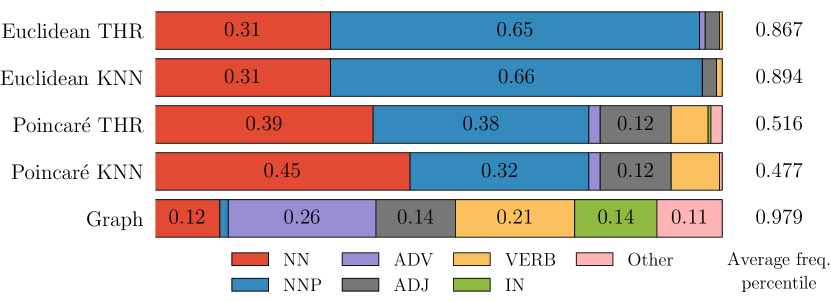
Figure 2: Top-200 words, the eigenvector centrality. POS distribution and the average frequency percentile.

A more robust measure of node importance is the eigenvector centrality (Bonacich, 1987). This centrality takes into account not only the degree of a node but also the importance of its neighbors: a high eigenvector score means that a node is connected to many nodes who themselves have high scores.

Figure 2 shows that for $G_{G}$ the top changes in a principled way: the average frequency increases, proper nouns almost vanish, many adverbs, prepositions, linking and introductory words appear (e.g., ‘well’, ‘but’, ‘in’, ‘that’). For $G_{G}$, the top consists of frequent generic words; this agrees with the intuitive understanding of importance. Differently from $G_{G}$, top words for $G_{E}$ and $G_{P}$ have lower frequencies, fewer adverbs and prepositions. This can be because it is hard to make generic words from different areas close for vector-based embeddings, while GraphGlove can learn arbitrary connections.

$k$-core.

	size	$k$
Euclidean	275	198
Poincaré	235	156
Graph	197	21

Table 5: The main core size and its $k$ value. For vector-based embeddings, the thr graphs are shown (by construction, the main core of a knn graph is trivial).

To further support this claim, we looked at the main $k$-core of the graphs. Formally, $k$-core is a maximal subgraph that contains nodes of degree $k$ or more; the main core is non-empty core with the largest $k$. Table 5 shows the sizes of the main cores and the corresponding values of $k$. Note that the maximum $k$ is much smaller for $G_{G}$; a possible explanation is that the cores in $G_{E}$ and $G_{P}$ are formed by nodes in highly dense regions of space, while in $G_{G}$ the most important nodes in different parts can be interlinked together.

5.2 The Structure is Hierarchical

In this section, we show that the structure of our graph reflects the hierarchical nature of words. We do so by comparing the structure learned by GraphGlove to the noun hierarchy from WordNet. To extract hierarchy from $G_{G}$, we (1) take all (lemmatized) nouns in our dataset which are also present in WordNet (22.5K words), (2) take the root noun ‘entity’ (which is the root of the WordNet tree), and (3) construct the hierarchy: the $k$-th level is formed by all nodes at edge distance $k$ from the root.

We consider two ways of measuring the agreement between the hierarchies: word correlation and level correlation. Word correlation is Spearman’s rank correlation between the vectors of levels for all nouns. Level correlation is Spearman’s rank correlation between the vectors $l$ and $l^{avg}$, where $l_{i}$ is the level in WordNet tree and $l_{i}^{avg}$ is the average level of $l_{i}$’s words in our hierarchy.

We performed these measurements for all graphs (see Table 6). We see that, according to both correlations, $G_{G}$ is in better agreement with the WordNet hierarchy.

		Word	Level
		correlation	correlation
Euclidean	thr	0.016	0.118
	knn	0.149	0.539
Poincaré	thr	0.018	0.122
	knn	0.124	0.094
Graph		0.199	0.650

Table 6: Correlations of hierarchies extracted from graphs and WordNet levels.

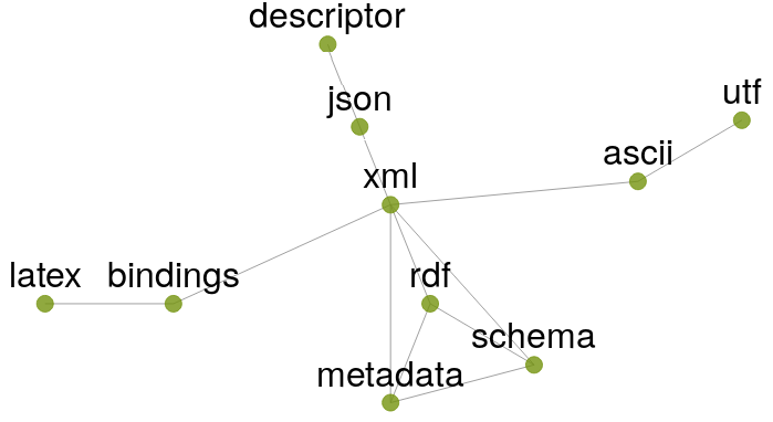
(a) $\delta\approx 0$

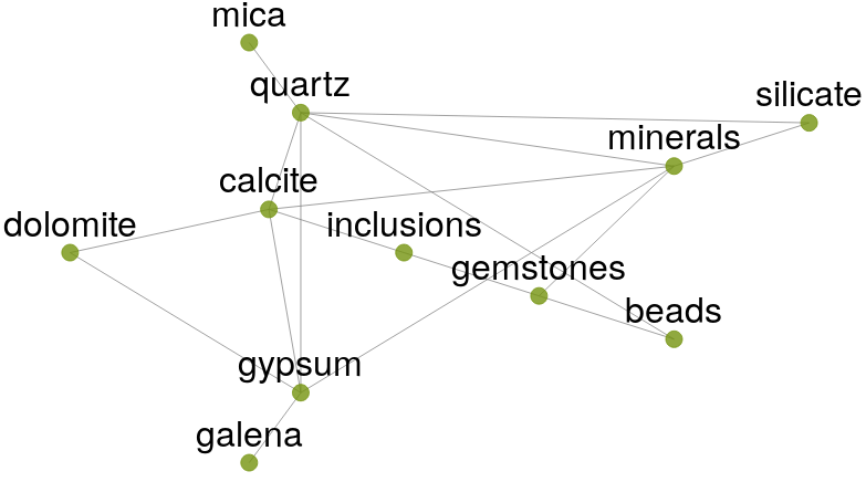
(b) $\delta\approx 0.15$

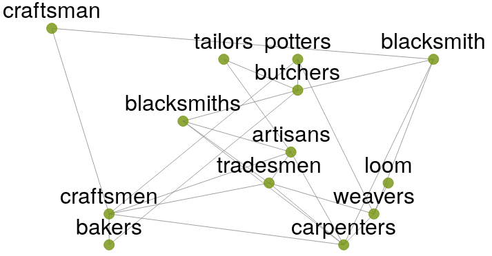
(c) $\delta\approx 0.35$

Figure 3: Examples of clusters with various $\delta$-hyperbolicities. For more interactive cluster visualizations, visit https://yandex-research.github.io/graph-glove/

5.3 The Geometry is Non-trivial

In contrast to vector embeddings, graph-based representations are not constrained by a vector space geometry and potentially can imitate arbitrarily complex spaces. Here we confirm that the geometry learned by GraphGlove is indeed non-trivial.

We cluster $G_{G}$ using the Chinese Whispers algorithm for graph node clustering (Biemann, 2006) and measure Gromov $\delta$-hyperbolicity for each cluster. Gromov hyperbolicity measures how close is a given metric to a tree metric (see, e.g., Tifrea et al. (2019) for the formal definition) and has previously been used to show the tree-like structure of the word log-co-occurrence graph Tifrea et al. (2019). Low average $\delta$ indicates tree-like structure with $\delta$ being exactly zero for trees; $\delta$ is usually normalized by the average shortest path length to get a value invariant to metric scaling.

Figure 4 shows the distribution of average $\delta$-hyperbolicity for clusters of size at least 10. Firstly, we see that for many clusters the normalized average $\delta$-hyperbolicity is close to zero, which agrees with the intuition that some words form a hierarchy. Secondly, $\delta$-hyperbolicity varies significantly over the clusters and some clusters have relatively large values; it means that these clusters are not tree-like. Figure 3 shows examples of clusters with different values of $\delta$-hyperbolicity: both tree-like (Figure 3a) and more complicated (Figure 3b-c).

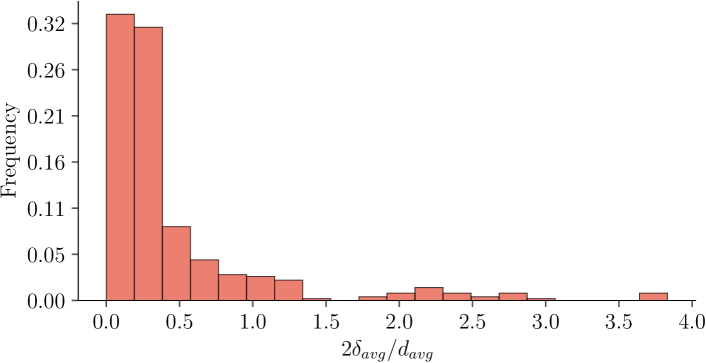
Figure 4: Distribution of cluster $\delta$-hyperbolicities, normalized by the average shortest path length in a cluster.

6 Related Work

Word embedding methods typically represent words as vectors in a low-dimensional space; usually, the vector space is Euclidean Mikolov et al. (2013b); Pennington et al. (2014); Bojanowski et al. (2017), but recently other spaces, e.g. hyperbolic, have been explored Leimeister and Wilson (2018); Dhingra et al. (2018); Tifrea et al. (2019). However, vectorial embeddings can have undesired properties: e.g., in dot product spaces certain words cannot be assigned high probability regardless of their context Demeter et al. (2020). A conceptually different approach is to model words as probability density functions Vilnis and McCallum (2015); Athiwaratkun and Wilson (2017); Bražinskas et al. (2018); Muzellec and Cuturi (2018); Athiwaratkun and Wilson (2018). We propose a new setting: embedding words as nodes in a weighted graph.

Representing language data in the form of a graph has been a long-standing task Miller (1995); Motter et al. (2002); Cancho and Solé (2001); Niyogi (2006); Masucci and Rodgers (2006). Graph lexicons were used to learn word embeddings specialized towards certain types of lexical knowledge Nguyen et al. (2017); Vulić and Mrkšić (2018); Liu et al. (2015); Ono et al. (2015); Mrkšić et al. (2017); Bollegala et al. (2016). It is also possible to incorporate external linguistic information from graphs, e.g. dependency parser outputs Vashishth et al. (2018).

To learn a weighted graph, we use the method by Mazur et al. (2019). Prior approaches to learning graphs from data are eigher highly problem-specific and not scalable Escolano and Hancock (2011); Karasuyama and Mamitsuka (2017); Kang et al. (2019) or solve a less general but important case of learning directed acyclic graphs Zheng et al. (2018); Yu et al. (2019). The opposite to learning a graph from data is the task of embedding nodes in a given graph to reflect graph distances and/or other properties; see Hamilton et al. (2017) for a thorough survey.

Analysis of word embeddings and the structure of the learned feature space often reveals interesting language properties and is an important research direction Köhn (2015); Bolukbasi et al. (2016); Mimno and Thompson (2017); Nakashole and Flauger (2018); Naik et al. (2019); Ethayarajh et al. (2019). We show that graph-based embeddings can be a powerful tool for language analysis.

7 Conclusions

We introduce GraphGlove — graph word embeddings, where each word is a node in a weighted graph and the distance between words is the shortest path distance between the corresponding nodes. The graph is learned end-to-end in an unsupervised manner. We show that GraphGlove substantially outperforms both Euclidean and Poincaré GloVe on word similarity and word analogy tasks. Our analysis reveals that the structure of the learned graphs is hierarchical and similar to that of WordNet; the geometry is highly non-trivial and contains subgraphs with different local topology.

Possible directions for future work include using GraphGlove for unsupervised hypernymy detection, analyzing undesirable word associations, comparing learned graph topologies for different languages, and downstream applications such as sequence classification. Also, given the recent success of models such as ELMo and BERT, it would be interesting to explore extensions of GraphGlove to the class of contextualized embeddings.

Appendix A Appendix: Additional benchmarks

A.1 Variance study

As our method relies on random initialization of a graph in PRODIGE, a natural question is whether different choice of drawn edges significantly affects the quality of representations in the end of training. Figure 5 demonstrates that after running the training procedure with distance-based loss for 5 different random seeds, the final metrics values have a standard deviation of less than 1 point in 10/13 tasks and have a standard deviation of at most 1.34 percent for the RareWord dataset. Thus, we can conclude that GraphGlove results are relatively stable with respect to selection of random edges before training.

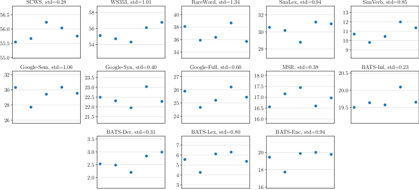
Figure 5: Results of evaluation for GraphGlove with 20 parameters per vertex on all benchmarks over 5 random initializations. Here, $d$ is used in the loss function.

A.2 Similarity

Below we report additional similarity benchmarks for GraphGlove and its vectorial counterparts:

• 50K tokens, 100 parameters / token - Table 7;

• 200K tokens, 20 parameters / token - Table 8.

Some word pairs in each similarity benchmark are out of vocabulary (OOV). In the main evaluation, we drop such pairs from the benchmark. However, there’s also a different way to deal with such words.

A popular workaround is to calculate the distance between $w_{i}$ and OOV as an average distance from $w_{i}$ to other words. In the rare case when both words are OOV, we can consider them infinitely distant from each other. We report similarity benchmarks including OOV tokens in Tables 9, 10 and 11.

		​​​​​​​SCWS	WS353	RW	SL	SV
Euclidean
		58.0	62.0	38.3	28.9	12.4
Poincaré
	$d^{2}$	53.2	57.3	40.8	29.4	12.56
	$\cosh^{2}d$	59.5	65.9	45.8	31.6	13.7
Graph
	$d$	59.3	65.5	46.0	33.6	12.6
	$\langle\cdot,\cdot\rangle$	56.8	61.6	42.6	32.8	14.8

Table 7: Spearman rank correlation on word similarity tasks. Models with 50k vocab., 100 parameters per token. Skip word pairs that contain OOV words.

		​​​​​​​SCWS	WS353	RW	SL	SV
Euclidean
		55.6	49.9	31.8	23.6	10.6
Poincaré
	$d^{2}$	46.2	45.0	28.5	23.5	12.0
	$\cosh^{2}d$	56.1	51.2	32.0	24.8	12.4
Graph
	$d$	58.5	56.4	33.4	23.4	11.5
	$\langle\cdot,\cdot\rangle$	53.2	52.9	30.9	23.4	13.8

Table 8: Spearman rank correlation on word similarity tasks. Models with 200k vocab., 20 parameters per token. Ignore word pairs with OOV words.

		​​​​​​​SCWS	WS353	RW	SL	SV
Euclidean
		50.5	44.9	11.5	19.5	6.7
Poincaré
	$d^{2}$	42.8	38.8	8.4	21.8	7.8
	$\cosh^{2}d$	49.8	49.8	11.6	22.3	8.3
Graph
	$d$	51.7	55.5	7.3	30.0	8.9
	$\langle\cdot,\cdot\rangle$	48.6	57.9	11.8	28.8	10.7

Table 9: Spearman rank correlation on word similarity tasks. Models with 50k vocab., 20 parameters per token. Infer distances to OOV words.

		​​​​​​​SCWS	WS353	RW	SL	SV
Euclidean
		54.2	58.8	9.2	27.8	8.8
Poincaré
	$d^{2}$	50.3	54.5	10.3	27.7	9.9
	$\cosh^{2}d$	55.4	60.1	12.8	29.6	10.0
Graph
	$d$	55.7	60.0	12.8	32.8	9.9
	$\langle\cdot,\cdot\rangle$	54.0	58.5	10.7	31.0	11.2

Table 10: Spearman rank correlation on word similarity tasks. Models with 50k vocab., 100 parameters per token. Infer distances to OOV words.

		​​​​​​​SCWS	WS353	RW	SL	SV
Euclidean
		54.4	49.9	24.9	23.7	10.8
Poincaré
	$d^{2}$	46.0	45.0	23.8	23.9	11.8
	$\cosh^{2}d$	56.0	51.2	27.5	24.9	12.3
Graph
	$d$	58.1	56.4	28.6	23.6	11.3
	$\langle\cdot,\cdot\rangle$	53.0	52.9	26.2	23.9	13.5

Table 11: Spearman rank correlation on word similarity tasks. Models with 200k vocab., 20 parameters per token. Infer distances to missing words.

A.3 Analogy

We also evaluate these scenarios for Analogy Prediction:

• 50K tokens, 100 parameters / token - Table 12;

• 200K tokens, 20 parameters / token - Table 13;

	Sem.	Syn.	Full	MSR
Euclidean
	61.6	50.0	55.1	48.0
Poincaré
$d^{2}$	49.4	38.3	43.2	26.1
$\cosh^{2}d$	63.2	56.8	59.6	47.8
Graph
$d$	59.9	58.3	59.0	46.0
$\langle\cdot,\cdot\rangle$	61.8	59.8	60.7	49.7

Table 12: Analogy prediction accuracy. Models with 50K tokens, 100 parameters per token.

	Sem.	Syn.	Full	MSR
Euclidean
	31.7	19.7	25.2	11.6
Poincaré
$d^{2}$	32.9	20.9	26.4	14.4
$\cosh^{2}d$	31.2	19.9	25.0	14.0
Graph
$d$	32.6	19.7	25.6	13.5
$\langle\cdot,\cdot\rangle$	34.3	24.7	29.1	19.7

Table 13: Analogy prediction accuracy. Models with 200K tokens, 20 parameters per token.

Appendix B Supplementary material: graph central nodes

Top 20 words by degree centrality

• Euclidean THR: [’cummings’, ’glover’, ’boyd’, ’hooper’, ’barrett’, ’hicks’, ’mckay’, ’dunn’, ’kemp’, ’moran’, ’payne’, ’ingram’, ’harrington’, ’webb’, ’ellis’, ’jenkins’, ’goodwin’, ’benson’, ’corbett’, ’willis’]

• Euclidean KNN: [’bunn’, ’willey’, ’cottrell’, ’sandys’, ’alfaro’, ’forgets’, ’ellis’, ’minaj’, ’taylor’, ’lemaire’, ’lockwood’, ’amused’, ’emiliano’, ’mckay’, ’boyd’, ’hurtado’, ’wonderfully’, ’russell’, ’this’, ’mundy’]

• Poincaré THR: [’mundy’, ’merriman’, ’hoskins’, ’cottrell’, ’oakes’, ’mayne’, ’griggs’, ’bunn’, ’hooper’, ’munn’, ’gillies’, ’glanville’, ’beal’, ’bartley’, ’halloran’, ’mcnab’, ’purdy’, ’bullard’, ’willett’, ’roper’]

• Poincaré KNN: [’imc’, ’cottrell’, ’willett’, ’foxy’, ’heim’, ’noa’, ’mundy’, ’newland’, ’bunn’, ’importantly’, ’krug’, ’grips’, ’hooper’, ’haney’, ’mcnab’, ’misplaced’, ’doty’, ’taki’, ’rushton’, ’likewise’]

• Graph: [’bennett’, ’even’, ’same’, ’allen’, ’james’, ’this’, ’although’, ’howard’, ’however’, ’particular’, ’example’, ’wilson’, ’robinson’, ’rather’, ’well’, ’only’, ’furthermore’, ’fact’, ’beginning’, ’smith’]

Top 20 words by eigenvector centrality

• Euclidean THR: [’dunn’, ’hooper’, ’boyd’, ’barrett’, ’jenkins’, ’ellis’, ’hicks’, ’webb’, ’payne’, ’cummings’, ’benson’, ’kemp’, ’willis’, ’glover’, ’mckay’, ’moran’, ’phillips’, ’steele’, ’chapman’, ’roberts’]

• Euclidean KNN: [’taylor’, ’ellis’, ’russell’, ’benson’, ’phillips’, ’thompson’, ’robinson’, ’moore’, ’roberts’, ’stevens’, ’allen’, ’curtis’, ’webb’, ’willis’, ’harvey’, ’chapman’, ’steele’, ’jones’, ’smith’, ’boyd’]

• Poincaré THR: [’hoskins’, ’oakes’, ’hooper’, ’gillies’, ’roper’, ’whitmore’, ’corrigan’, ’waddell’, ’metcalfe’, ’goodwin’, ’bowles’, ’mundy’, ’sanderson’, ’kemp’, ’tobin’, ’merriman’, ’harrington’, ’mccallum’, ’cartwright’, ’halloran’]

• Poincaré KNN: [’willett’, ’cottrell’, ’bunn’, ’rushton’, ’doty’, ’mundy’, ’munn’, ’brower’, ’rowell’, ’glanville’, ’macklin’, ’purnell’, ’mcnab’, ’clapp’, ’tasker’, ’treadwell’, ’nichol’, ’newland’, ’willey’, ’prichard’]

• Graph: [’even’, ’same’, ’however’, ’this’, ’only’, ’although’, ’well’, ’another’, ’both’, ’in’, ’while’, ’rather’, ’fact’, ’that’, ’once’, ’though’, ’furthermore’, ’taken’, ’but’, ’particular’]

Main $k$-cores

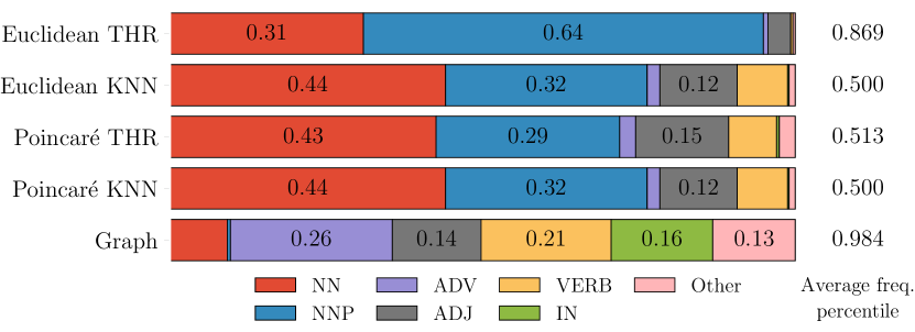
Figure 6: POS distribution for main k-core

• Euclidean THR: [’nathan’, ’harold’, ’dick’, ’sullivan’, ’donaldson’, ’yates’, ’kerr’, ’terry’, ’byron’, ’duncan’, ’horton’, ’kelley’, ’parker’, ’oliver’, ’duffy’, ’mclean’, ’jeremy’, ’bartlett’, ’osborne’, ’howell’, ’webb’, ’hughes’, ’gould’, ’pearce’, ’bradley’, ’walker’, ’barry’, ’davidson’, ’graham’, ’jesse’, ’blair’, ’collins’, ’bailey’, ’burnett’, ’harrington’, ’cole’, ’wilson’, ’jonathan’, ’gary’, ’tim’, ’leslie’, ’cunningham’, ’elliot’, ’jones’, ’gorman’, ’holt’, ’lynch’, ’holloway’, ’wheeler’, ’reid’, ’cox’, ’evan’, ’freeman’, ’burgess’, ’barker’, ’skinner’, ’baxter’, ’hayes’, ’amos’, ’colin’, ’ritchie’, ’harry’, ’campbell’, ’nolan’, ’howard’, ’simpson’, ’mckenzie’, ’ralph’, ’gibson’, ’rowland’, ’lynn’, ’jarvis’, ’chandler’, ’dawson’, ’trevor’, ’carter’, ’stevens’, ’nichols’, ’hurley’, ’hines’, ’steele’, ’payne’, ’shaw’, ’phillip’, ’henderson’, ’richardson’, ’andrews’, ’anthony’, ’briggs’, ’roberts’, ’fletcher’, ’mccall’, ’gallagher’, ’robertson’, ’fowler’, ’lowe’, ’harris’, ’johnson’, ’willis’, ’carr’, ’goodwin’, ’spencer’, ’neil’, ’noel’, ’tucker’, ’atkins’, ’dixon’, ’miller’, ’bates’, ’sweeney’, ’barlow’, ’andrew’, ’wright’, ’reeves’, ’glover’, ’irwin’, ’phillips’, ’hanson’, ’dillon’, ’mitchell’, ’armstrong’, ’farrell’, ’stevenson’, ’nicholson’, ’stewart’, ’baker’, ’norris’, ’coleman’, ’hicks’, ’foley’, ’jack’, ’wilkinson’, ’powell’, ’nelson’, ’dalton’, ’lewis’, ’murray’, ’boyd’, ’watson’, ’elliott’, ’hobbs’, ’turner’, ’horne’, ’derek’, ’walters’, ’daly’, ’fleming’, ’curtis’, ’scott’, ’wallace’, ’alan’, ’bennett’, ’stephens’, ’laurie’, ’leonard’, ’barnett’, ’murphy’, ’stuart’, ’crawford’, ’dunn’, ’kemp’, ’lester’, ’ingram’, ’connor’, ’donald’, ’mckay’, ’bruce’, ’hale’, ’kirk’, ’williamson’, ’robinson’, ’russell’, ’barr’, ’jim’, ’abbott’, ’donovan’, ’morris’, ’dickson’, ’burke’, ’chapman’, ’keith’, ’morrison’, ’hartley’, ’cameron’, ’dennis’, ’allen’, ’bradshaw’, ’thornton’, ’gardner’, ’townsend’, ’evans’, ’richards’, ’steve’, ’griffin’, ’frank’, ’atkinson’, ’wills’, ’donnell’, ’doyle’, ’moran’, ’palmer’, ’reynolds’, ’bowen’, ’bryan’, ’slater’, ’edwards’, ’fisher’, ’clarke’, ’ramsey’, ’brooks’, ’cooper’, ’gordon’, ’harvey’, ’morgan’, ’ferguson’, ’ross’, ’chris’, ’fred’, ’smith’, ’tom’, ’david’, ’cooke’, ’benson’, ’haynes’, ’butler’, ’cummings’, ’matthews’, ’perkins’, ’hooper’, ’taylor’, ’brian’, ’jenkins’, ’buckley’, ’hawkins’, ’randall’, ’michael’, ’rogers’, ’mcintyre’, ’ted’, ’phil’, ’johnston’, ’cullen’, ’kelly’, ’corbett’, ’eric’, ’clark’, ’owen’, ’rowe’, ’connolly’, ’moore’, ’garrett’, ’thompson’, ’patrick’, ’stephen’, ’wade’, ’brien’, ’barrett’, ’hart’, ’saunders’, ’james’, ’nash’, ’watkins’, ’ellis’, ’walsh’, ’mason’, ’todd’, ’barnes’, ’jennings’, ’patterson’, ’connell’, ’lawson’, ’craig’, ’rodney’, ’blake’, ’adams’]

• Poincaré THR: [’nichols’, ’mcintyre’, ’randall’, ’mckay’, ’perkins’, ’noel’, ’elliott’, ’reynolds’, ’richards’, ’glenn’, ’lester’, ’foley’, ’walsh’, ’murray’, ’fitzgerald’, ’donovan’, ’riley’, ’thornton’, ’kemp’, ’rodney’, ’bartlett’, ’kirk’, ’bradley’, ’curtis’, ’jenkins’, ’roberts’, ’hayden’, ’byron’, ’skinner’, ’smith’, ’horton’, ’carr’, ’yates’, ’chapman’, ’benson’, ’wilkinson’, ’marshall’, ’connor’, ’bruce’, ’barnett’, ’quinn’, ’fleming’, ’barry’, ’payne’, ’carter’, ’richardson’, ’tanner’, ’watson’, ’freeman’, ’buckley’, ’simpson’, ’watkins’, ’owen’, ’todd’, ’miller’, ’shaw’, ’gibson’, ’baker’, ’ritchie’, ’hooper’, ’mason’, ’osborne’, ’lawson’, ’harrington’, ’jeremy’, ’kerr’, ’patterson’, ’simmons’, ’warren’, ’wallace’, ’jarvis’, ’gardner’, ’reilly’, ’harvey’, ’henderson’, ’coleman’, ’barrett’, ’leonard’, ’saunders’, ’glover’, ’hughes’, ’farrell’, ’anthony’, ’fisher’, ’cox’, ’goodwin’, ’bowman’, ’mitchell’, ’daniels’, ’sullivan’, ’griffin’, ’abbott’, ’morris’, ’peterson’, ’reeves’, ’ralph’, ’ross’, ’elliot’, ’brien’, ’howard’, ’donaldson’, ’walters’, ’russell’, ’andrew’, ’burke’, ’edwards’, ’dunn’, ’phillips’, ’hurley’, ’lynch’, ’rogers’, ’barnes’, ’doyle’, ’harris’, ’evans’, ’stewart’, ’stevenson’, ’sheldon’, ’burnett’, ’connolly’, ’burgess’, ’cummings’, ’williamson’, ’wilson’, ’steele’, ’irwin’, ’hicks’, ’cooke’, ’hanson’, ’matthews’, ’hawkins’, ’gorman’, ’willis’, ’palmer’, ’cameron’, ’hayes’, ’daly’, ’morrison’, ’moran’, ’haynes’, ’taylor’, ’gordon’, ’cunningham’, ’stevens’, ’dawson’, ’clarke’, ’morgan’, ’robertson’, ’mclean’, ’thompson’, ’spencer’, ’murphy’, ’davidson’, ’duncan’, ’evan’, ’johnston’, ’hart’, ’terry’, ’fletcher’, ’spence’, ’connell’, ’griffith’, ’parsons’, ’allen’, ’ellis’, ’reid’, ’adams’, ’jones’, ’nathan’, ’norris’, ’pearce’, ’ingram’, ’brooks’, ’dillon’, ’cooper’, ’keith’, ’crawford’, ’hale’, ’parker’, ’webb’, ’baxter’, ’blake’, ’turner’, ’craig’, ’fuller’, ’nicholson’, ’barker’, ’campbell’, ’fred’, ’bailey’, ’grady’, ’nolan’, ’welch’, ’powell’, ’armstrong’, ’dalton’, ’gavin’, ’sanders’, ’trevor’, ’duffy’, ’brent’, ’dale’, ’hoffman’, ’garrett’, ’boyd’, ’robinson’, ’dennis’, ’jennings’, ’clark’, ’graham’, ’kelley’, ’newman’, ’rowe’, ’scott’, ’phillip’, ’porter’, ’wright’, ’ferguson’, ’clayton’, ’dixon’, ’briggs’, ’howell’, ’mckenzie’, ’chandler’, ’collins’, ’lewis’, ’gallagher’, ’mcbride’, ’fowler’, ’harding’, ’flynn’, ’lowe’, ’moore’, ’walker’, ’bennett’]

• Graph: [’more’, ’being’, ’took’, ’while’, ’seen’, ’under’, ’never’, ’are’, ’by’, ’furthermore’, ’though’, ’at’, ’presumably’, ’finally’, ’then’, ’ones’, ’was’, ’initially’, ’these’, ’their’, ’among’, ’together’, ’or’, ’also’, ’included’, ’few’, ’up’, ’earlier’, ’even’, ’existed’, ’longer’, ’first’, ’be’, ’beginning’, ’hence’, ’notably’, ’the’, ’well’, ’will’, ’similarly’, ’actually’, ’different’, ’around’, ’them’, ’unlike’, ’several’, ’now’, ’once’, ’such’, ’prior’, ’fact’, ’other’, ’both’, ’for’, ’only’, ’next’, ’therefore’, ’two’, ’had’, ’along’, ’part’, ’times’, ’because’, ’likewise’, ’latter’, ’since’, ’additionally’, ’to’, ’where’, ’still’, ’than’, ’but’, ’end’, ’taken’, ’instance’, ’addition’, ’having’, ’after’, ’same’, ’despite’, ’of’, ’similar’, ’over’, ’during’, ’one’, ’appear’, ’outside’, ’much’, ’nevertheless’, ’came’, ’make’, ’have’, ’some’, ’those’, ’usually’, ’it’, ’this’, ’number’, ’when’, ’separate’, ’moreover’, ’following’, ’saw’, ’with’, ’time’, ’before’, ’full’, ’within’, ’perhaps’, ’any’, ’rest’, ’might’, ’others’, ’exception’, ’as’, ’using’, ’instances’, ’is’, ’making’, ’found’, ’made’, ’use’, ’come’, ’without’, ’until’, ’should’, ’example’, ’through’, ’so’, ’itself’, ’although’, ’its’, ’that’, ’throughout’, ’besides’, ’they’, ’consequently’, ’ever’, ’given’, ’and’, ’just’, ’not’, ’afterwards’, ’there’, ’added’, ’years’, ’on’, ’later’, ’however’, ’could’, ’ended’, ’indeed’, ’all’, ’went’, ’believed’, ’take’, ’rather’, ’in’, ’already’, ’every’, ’set’, ’either’, ’entered’, ’possible’, ’an’, ’themselves’, ’often’, ’would’, ’which’, ’instead’, ’second’, ’last’, ’each’, ’thus’, ’again’, ’certain’, ’most’, ’old’, ’from’, ’were’, ’yet’, ’likely’, ’elsewhere’, ’been’, ’way’, ’new’, ’what’, ’own’, ’has’, ’out’, ’if’, ’another’, ’many’, ’particular’, ’taking’, ’can’, ’today’]

References

- Athiwaratkun and Wilson (2017) Ben Athiwaratkun and Andrew Wilson. 2017. Multimodal word distributions. In Proceedings of the 55th Annual Meeting of the Association for Computational Linguistics (Volume 1: Long Papers), pages 1645–1656, Vancouver, Canada. Association for Computational Linguistics.
- Athiwaratkun and Wilson (2018) Ben Athiwaratkun and Andrew Gordon Wilson. 2018. On modeling hierarchical data via probabilistic order embeddings. In International Conference on Learning Representations.
- Biemann (2006) Chris Biemann. 2006. Chinese whispers: an efficient graph clustering algorithm and its application to natural language processing problems. In Proceedings of the first workshop on graph based methods for natural language processing, pages 73–80. Association for Computational Linguistics.
- Bojanowski et al. (2017) Piotr Bojanowski, Edouard Grave, Armand Joulin, and Tomas Mikolov. 2017. Enriching word vectors with subword information. Transactions of the Association for Computational Linguistics, 5:135–146.
- Bollegala et al. (2016) Danushka Bollegala, Mohammed Alsuhaibani, Takanori Maehara, and Ken-ichi Kawarabayashi. 2016. Joint word representation learning using a corpus and a semantic lexicon. In Thirtieth AAAI Conference on Artificial Intelligence.
- Bolukbasi et al. (2016) Tolga Bolukbasi, Kai-Wei Chang, James Y Zou, Venkatesh Saligrama, and Adam T Kalai. 2016. Man is to computer programmer as woman is to homemaker? debiasing word embeddings. In Advances in neural information processing systems, pages 4349–4357.
- Bonacich (1987) Phillip Bonacich. 1987. Power and centrality: A family of measures. American journal of sociology, 92(5):1170–1182.
- Bražinskas et al. (2018) Arthur Bražinskas, Serhii Havrylov, and Ivan Titov. 2018. Embedding words as distributions with a Bayesian skip-gram model. In Proceedings of the 27th International Conference on Computational Linguistics, pages 1775–1789, Santa Fe, New Mexico, USA. Association for Computational Linguistics.
- Cancho and Solé (2001) Ramon Ferrer I Cancho and Richard V Solé. 2001. The small world of human language. Proceedings of the Royal Society of London. Series B: Biological Sciences, 268(1482):2261–2265.
- Demeter et al. (2020) David Demeter, Gregory Kimmel, and Doug Downey. 2020. Stolen probability: A structural weakness of neural language models.
- Dhingra et al. (2018) Bhuwan Dhingra, Christopher Shallue, Mohammad Norouzi, Andrew Dai, and George Dahl. 2018. Embedding text in hyperbolic spaces. In Proceedings of the Twelfth Workshop on Graph-Based Methods for Natural Language Processing (TextGraphs-12), pages 59–69, New Orleans, Louisiana, USA. Association for Computational Linguistics.
- Escolano and Hancock (2011) Francisco Escolano and Edwin R Hancock. 2011. From points to nodes: Inverse graph embedding through a lagrangian formulation. In International Conference on Computer Analysis of Images and Patterns, pages 194–201. Springer.
- Ethayarajh et al. (2019) Kawin Ethayarajh, David Duvenaud, and Graeme Hirst. 2019. Understanding undesirable word embedding associations. In Proceedings of the 57th Annual Meeting of the Association for Computational Linguistics, pages 1696–1705, Florence, Italy. Association for Computational Linguistics.
- Gladkova et al. (2016) Anna Gladkova, Aleksandr Drozd, and Satoshi Matsuoka. 2016. Analogy-based detection of morphological and semantic relations with word embeddings: What works and what doesn’t. In Proceedings of the NAACL-HLT SRW, pages 47–54, San Diego, California, June 12-17, 2016. ACL.
- Glynn (1990) Peter W Glynn. 1990. Likelihood ratio gradient estimation for stochastic systems. Communications of the ACM.
- Gu et al. (2018) Albert Gu, Frederic Sala, Beliz Gunel, and Christopher Ré. 2018. Learning mixed-curvature representations in product spaces. In International Conference on Learning Representations.
- Hamilton et al. (2017) William L Hamilton, Rex Ying, and Jure Leskovec. 2017. Representation learning on graphs: Methods and applications. arXiv preprint arXiv:1709.05584.
- Kang et al. (2019) Zhao Kang, Haiqi Pan, Steven CH Hoi, and Zenglin Xu. 2019. Robust graph learning from noisy data. IEEE transactions on cybernetics.
- Karasuyama and Mamitsuka (2017) Masayuki Karasuyama and Hiroshi Mamitsuka. 2017. Adaptive edge weighting for graph-based learning algorithms. Machine Learning, 106(2):307–335.
- Kingma and Ba (2014) Diederik Kingma and Jimmy Ba. 2014. Adam: A method for stochastic optimization. International Conference on Learning Representations.
- Köhn (2015) Arne Köhn. 2015. What’s in an embedding? analyzing word embeddings through multilingual evaluation. In Proceedings of the 2015 Conference on Empirical Methods in Natural Language Processing, pages 2067–2073, Lisbon, Portugal. Association for Computational Linguistics.
- Leimeister and Wilson (2018) Matthias Leimeister and Benjamin J Wilson. 2018. Skip-gram word embeddings in hyperbolic space. arXiv preprint arXiv:1809.01498.
- Liu et al. (2015) Quan Liu, Hui Jiang, Si Wei, Zhen-Hua Ling, and Yu Hu. 2015. Learning semantic word embeddings based on ordinal knowledge constraints. In Proceedings of the 53rd Annual Meeting of the Association for Computational Linguistics and the 7th International Joint Conference on Natural Language Processing (Volume 1: Long Papers), pages 1501–1511, Beijing, China. Association for Computational Linguistics.
- Masucci and Rodgers (2006) Adolfo Paolo Masucci and Geoff J Rodgers. 2006. Network properties of written human language. Physical Review E, 74(2):026102.
- Mazur et al. (2019) Denis Mazur, Vage Egiazarian, Stanislav Morozov, and Artem Babenko. 2019. Beyond vector spaces: Compact data representation as differentiable weighted graphs. In NeurIPS, Vancouver, Canada.
- Mikolov et al. (2013a) Tomas Mikolov, Kai Chen, Greg Corrado, and Jeffrey Dean. 2013a. Efficient estimation of word representations in vector space. arXiv preprint arXiv:1301.3781.
- Mikolov et al. (2013b) Tomas Mikolov, Ilya Sutskever, Kai Chen, Greg S Corrado, and Jeff Dean. 2013b. Distributed representations of words and phrases and their compositionality. In Advances in Neural Information Processing Systems 26, pages 3111–3119.
- Mikolov et al. (2013c) Tomas Mikolov, Wen-tau Yih, and Geoffrey Zweig. 2013c. Linguistic regularities in continuous space word representations. In Proceedings of the 2013 Conference of the North American Chapter of the Association for Computational Linguistics: Human Language Technologies, pages 746–751, Atlanta, Georgia. Association for Computational Linguistics.
- Miller (1995) George A Miller. 1995. Wordnet: a lexical database for english. Communications of the ACM, 38(11):39–41.
- Mimno and Thompson (2017) David Mimno and Laure Thompson. 2017. The strange geometry of skip-gram with negative sampling. In Proceedings of the 2017 Conference on Empirical Methods in Natural Language Processing, pages 2873–2878, Copenhagen, Denmark. Association for Computational Linguistics.
- Motter et al. (2002) Adilson E Motter, Alessandro PS De Moura, Ying-Cheng Lai, and Partha Dasgupta. 2002. Topology of the conceptual network of language. Physical Review E, 65(6):065102.
- Mrkšić et al. (2017) Nikola Mrkšić, Ivan Vulić, Diarmuid Ó Séaghdha, Ira Leviant, Roi Reichart, Milica Gašić, Anna Korhonen, and Steve Young. 2017. Semantic specialization of distributional word vector spaces using monolingual and cross-lingual constraints. Transactions of the Association for Computational Linguistics, 5:309–324.
- Muzellec and Cuturi (2018) Boris Muzellec and Marco Cuturi. 2018. Generalizing point embeddings using the wasserstein space of elliptical distributions. In Advances in Neural Information Processing Systems, pages 10237–10248.
- Naik et al. (2019) Aakanksha Naik, Abhilasha Ravichander, Carolyn Rose, and Eduard Hovy. 2019. Exploring numeracy in word embeddings. In Proceedings of the 57th Annual Meeting of the Association for Computational Linguistics, pages 3374–3380, Florence, Italy. Association for Computational Linguistics.
- Nakashole and Flauger (2018) Ndapa Nakashole and Raphael Flauger. 2018. Characterizing departures from linearity in word translation. In Proceedings of the 56th Annual Meeting of the Association for Computational Linguistics (Volume 2: Short Papers), pages 221–227, Melbourne, Australia. Association for Computational Linguistics.
- Nguyen et al. (2017) Kim Anh Nguyen, Maximilian Köper, Sabine Schulte im Walde, and Ngoc Thang Vu. 2017. Hierarchical embeddings for hypernymy detection and directionality. In Proceedings of the 2017 Conference on Empirical Methods in Natural Language Processing, pages 233–243, Copenhagen, Denmark. Association for Computational Linguistics.
- Niyogi (2006) Partha Niyogi. 2006. The computational nature of language learning and evolution. MIT press Cambridge, MA.
- Ono et al. (2015) Masataka Ono, Makoto Miwa, and Yutaka Sasaki. 2015. Word embedding-based antonym detection using thesauri and distributional information. In Proceedings of the 2015 Conference of the North American Chapter of the Association for Computational Linguistics: Human Language Technologies, pages 984–989, Denver, Colorado. Association for Computational Linguistics.
- Pennington et al. (2014) Jeffrey Pennington, Richard Socher, and Christopher Manning. 2014. Glove: Global vectors for word representation. In Proceedings of the 2014 Conference on Empirical Methods in Natural Language Processing (EMNLP), pages 1532–1543, Doha, Qatar. Association for Computational Linguistics.
- Tifrea et al. (2019) Alexandru Tifrea, Gary Becigneul, and Octavian-Eugen Ganea. 2019. Poincare glove: Hyperbolic word embeddings. In International Conference on Learning Representations.
- Vashishth et al. (2018) Shikhar Vashishth, Manik Bhandari, Prateek Yadav, Piyush Rai, Chiranjib Bhattacharyya, and Partha Talukdar. 2018. Incorporating syntactic and semantic information in word embeddings using graph convolutional networks.
- Vilnis and McCallum (2015) Luke Vilnis and Andrew McCallum. 2015. Word representations via gaussian embedding. In International Conference on Learning Representations.
- Vulić and Mrkšić (2018) Ivan Vulić and Nikola Mrkšić. 2018. Specialising word vectors for lexical entailment. In Proceedings of the 2018 Conference of the North American Chapter of the Association for Computational Linguistics: Human Language Technologies, Volume 1 (Long Papers), pages 1134–1145, New Orleans, Louisiana. Association for Computational Linguistics.
- Yu et al. (2019) Yue Yu, Jie Chen, Tian Gao, and Mo Yu. 2019. Dag-gnn: Dag structure learning with graph neural networks. arXiv preprint arXiv:1904.10098.
- Zheng et al. (2018) Xun Zheng, Bryon Aragam, Pradeep K Ravikumar, and Eric P Xing. 2018. Dags with no tears: Continuous optimization for structure learning. In Advances in Neural Information Processing Systems, pages 9472–9483.