Scene Graph Modification Based on Natural Language Commands

Abstract

Structured representations like graphs and parse trees play a crucial role in many Natural Language Processing systems. In recent years, the advancements in multi-turn user interfaces necessitate the need for controlling and updating these structured representations given new sources of information. Although there have been many efforts focusing on improving the performance of the parsers that map text to graphs or parse trees, very few have explored the problem of directly manipulating these representations. In this paper, we explore the novel problem of graph modification, where the systems need to learn how to update an existing scene graph given a new user’s command. Our novel models based on graph-based sparse transformer and cross attention information fusion outperform previous systems adapted from the machine translation and graph generation literature. We further contribute our large graph modification datasets to the research community to encourage future research for this new problem.

1 Introduction

Parsing text into structured semantics representation is one of the most long-standing and active research problems in NLP. Numerous parsing methods have been developed for many different semantic structure representations Chen and Manning (2014); Mrini et al. (2019); Zhou and Zhao (2019); Clark et al. (2018); Wang et al. (2018). However, most of these previous works focus on parsing a single sentence, while a typical human-computer interaction session or conversation is not single-turn. A prominent example is image search. Users usually start with short phrases describing the main objects or topics they are looking for. Depending on the result, the users may then modify their query to add more constraints or give additional information. In this case, without the modification capability, a static representation is not suitable to track the changing intent of the user. We argue that the back-and-forth and multi-turn nature of human-computer interactions necessitate the need for updating the structured representation. Another advantage of modifying a structured representation in the interactive setting is that it makes it easier to check the consistency. For instance, it is much easier to check whether the user requests two contradicting attributes for the same object in a scene graph during the interactive search, which can be done automatically.

In this paper, we propose the problem of scene graph modification for search. A scene graph Johnson et al. (2015) is a semantic formalism which represents the desired image as a graph of objects with relations and attributes. This semantic representation has been shown to be very successful in retrieval systems Johnson et al. (2015); Schuster et al. (2015); Vendrov et al. (2015). Inspired by the dialog state tracking setting Perez and Liu (2017); Ren et al. (2018), we consider the scene graph modification problem as follows. Given an initial scene graph and a new query issued by the user, the goal is to generate a new scene graph taking into account the original graph and the new query.

We formulate the problem as conditional graph modification, and create three datasets for this problem. We propose novel encoder-decoder architectures for conditional graph modification. More specifically, our graph encoder is built upon the self-attention architecture popular in state-of-the-art machine translation models Vaswani et al. (2017); Edunov et al. (2018), which is superior to, according to our study, Graph Convolutional Networks (GCN)  Kipf and Welling (2016). Unique to our problem, however, is the fact that we have an open set of relation types in the graphs. Thus, we propose a novel graph-conditioned sparse transformer, in which the relation information is embedded directly into the self-attention grid. For the decoder, we treat the graph modification task as a sequence generation problem  Li et al. (2018); Simonovsky and Komodakis (2018); You et al. (2018). Furthermore, to encourage the information sharing between the input graph and modification query, we introduce two techniques, i.e. late feature fusion through gating and early feature fusion through cross-attention. We further create three datasets to evaluate our models. The first two datasets are derived from public sources: MSCOCO Lin et al. (2014) and Google Conceptual Captioning (GCC) Sharma et al. (2018) while the last is collected using Amazon Mechanical Turk (MTurk). Experiments show that our best model achieves up to 8.5% improvement over the strong baselines on both the synthetic and user-generated data in terms of F1 score.

Our contributions are three-fold. Firstly, we introduce the problem of scene graph modification – an important component in multi-modal search and dialogue. Secondly, we propose a novel encoder-decoder architecture relying on graph-conditioned transformer and cross-attention to tackle the problem, outperforming strong baselines which we setup for the task. Thirdly, we introduce three datasets which can serve as evaluation benchmarks for future research.

2 Data Creation

In this section, we detail our data creation process. We start with information on scene graphs and a parser to generate them for the captions in two existing datasets, i.e. MSCOCO Lin et al. (2014) and GCC Sharma et al. (2018). We then describe how to generate modified scene graphs and modification queries based on these scene graphs, and leverage human annotators to increase and analyze data quality.

2.1 Scene Graphs

Schuster et al. (2015) introduce scene graphs as semantic representations of images. As shown in Figure 1, a parser will parse a sentence into a list of objects, e.g. ”boy” and ”shirt”. These objects and their associated attributes and relations form a group of triplets, e.g. $\langle boy,in,shirt\rangle$, $\langle boy,attribute,young\rangle$ and $\langle shirt,attribute,black\rangle$.

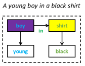
Figure 1: Example scene graph

Although there are several scene graphs annotated datasets for images Krishna et al. (2017), the alignments between graphs and text are unavailable. Moreover, image grounded scene graphs, e.g. the Visual Genome dataset Krishna et al. (2017), also contain lots of non-salient objects and relations, while search queries focus more on the main objects and their connections.

The lack of a large-scale and high quality public dataset prompts us to create our own benchmark datasets. To do this, we start with the popular captioning datasets: MSCOCO Lin et al. (2014) and GCC Sharma et al. (2018). To construct scene graphs, we use an in-house scene graph parser to parse a random subset of MSCOCO description data and GCC captions. The parser is built upon a dependency parser Dozat and Manning (2016), similar to the SPICE system Anderson et al. (2016).

2.2 Modified MSCOCO and GCC for Graph Modification

Our first two datasets add annotations on top of the captions for MSCOCO and GCC. The parser described in §2.1 is used to create 200k scene graphs from MSCOCO and 420k scene graphs from GCC data. Comparing the two datasets, the graphs from MSCOCO are simpler, while the GCC graphs are much more complicated. According to our in-house search log, image search queries are usually short, thus the MSCOCO graphs represents a closer match to actual search queries, while the GCC graphs present a greater challenge to the models.

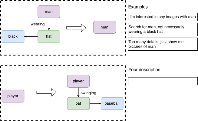
Figure 2: An interface of the crowd-sourcing stage

Given a scene graph $\mathcal{G}$, we construct a triplet $(\boldsymbol{\mathbf{x}},\boldsymbol{\mathbf{y}},\boldsymbol{\mathbf{z}})$, where $\boldsymbol{\mathbf{x}}$ is the source graph, $\boldsymbol{\mathbf{y}}$ indicates the modification query, and $\boldsymbol{\mathbf{z}}$ represents the target graph. More specifically, we uniformly select and apply an action $\boldsymbol{\mathbf{a}}$ from the set of all possible graph modification operations $A=\{\textsc{Insert},\textsc{Delete},\textsc{Substitute}\}$. The actions are applied to the graph as follows:

Delete.

We randomly select a node from $\mathcal{G}$ (denoting the source graph $\boldsymbol{\mathbf{x}}$), and then remove this node and its associated edges. The remaining nodes and edges are then the target graph $\boldsymbol{\mathbf{z}}$. As for the modification query $\boldsymbol{\mathbf{y}}$, it is generated from a randomly selected deletion template or by MTurk workers. These templates are based upon the Edit Me dataset Manuvinakurike et al. (2018).

Insert.

We treat insertion as the inversion of deletion. Specifically, we produce the source graph $\boldsymbol{\mathbf{x}}$ via a Delete operation on $\mathcal{G}$, where the target graph $\boldsymbol{\mathbf{z}}$ is set to $\mathcal{G}$. Like the deletion operator, the insertion query $\boldsymbol{\mathbf{y}}$ is generated by either the MTurk workers, or by templates.

Substitute.

We replace a randomly selected node from the source graph $\mathcal{G}$ with a semantically similar node to get the target graph. To find the new node, we make use of the AllenNLP toolkit Gardner et al. (2017) to get a list of candidate words based on their semantic similarity scores to the old node. More details can be found in our supplementary materials.

2.3 Crowd-sourcing User Data

As described above, apart from using templates, we crowd-source more diverse and natural modification queries from MTurk. As depicted in figure 2, we first show the workers an example which includes a source graph, a target graph and three acceptable modification queries. Then the workers are asked to fill in their own description for the unannotated instances. We refer to the template-based version of the datasets as “synthetic” while the user-generated contents as “user-generated”.

From our preliminary trials, we notice several difficulties within the data collection process. Firstly, understanding the graphs requires some knowledge of NLP, thus not all MTurk workers can provide good modification queries. Secondly, due to deletion and parser errors, we encounter some graphs with disconnected components in the data. Thirdly, there are many overly complicated graphs which are not representative of search queries, as most of the search queries are relatively short, with just one or two objects. To mitigate these problems, we manually filter the data by removing graphs with disconnected components, low-quality instances, or excessively long descriptions (i.e. more than 5 nodes). The final dataset contains 32k examples.

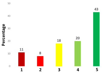
Figure 3: Quality score distribution.

To test the quality of our crowd-sourced dataset, we perform a limited user study with 15 testers who are not aware of the nature of the work and how we collect the dataset. We give them a random collection of instances, each of which is a triplet of source graph, modification query, and target graph. The tester would then give a score indicating the quality of each instance based on the following two criteria: (i) how well the modification query is reflected in the target graph? and (2) how natural are the query and the graphs? Regarding the second criterion, we instruct the scorer to assess whether the query and graph are human-like, grammatically and semantically. Furthermore, as most scorers are knowledgeable in image search, they are also required to evaluate whether they think the query is plausible in a search scenario.

Figure 3 shows the score distribution from 200 randomly chosen instances. We observe that most of the quality scores of 3 or 4 are due to the modification query or graphs to be unnatural. Testers tend to give the score of 1 for semantically wrong instances (e.g the modification query does not match the changes). Overall, the testers judge the data to be good with the average score of 3.76.

2.4 Extension: Multiple Operations

In §2.3, we have introduced our basic modification operations. From the analysis of our in-house search log, more than 95% of the queries have only one or two nodes, thus a scenario in which more than one edit operation applied is unlikely. Consequently, the instances in Modified MSCOCO and GCC are constructed with one edit operation. However, in some cases, there can be a very long search description , which leads to the possibility of longer edit operation sequences. This motivates us to create the multi-operation version of a dataset, i.e. the multi-operation graph modification (MGM) task from GCC data. Please refer to the supplementary material for the details of the data creation for MGM.

3 Methodology

In this section, we explore different methods to tackle our proposed problem. By analyzing the results and comparing different models, we establish baselines and set up the research direction for future work. We start by formalizing the problem, and defining the input as well as the expected output along with the notations. We then define our encoder-decoder architecture with the focus on our novel modeling characteristics: (i) the graph encoder with graph-conditioned, sparsely connected transformer and (ii) the early and late feature fusion models for combining information from the input text and graph.

Notations.

A graph is represented by $\boldsymbol{\mathbf{x}}^{\mathcal{G}}:=(\boldsymbol{\mathbf{x}}^{\mathcal{N}},\boldsymbol{\mathbf{x}}^{\mathcal{E}})$. The node set is denoted by $\boldsymbol{\mathbf{x}}^{\mathcal{N}}:=\{x_{1},..,x_{|\boldsymbol{\mathbf{x}}^{\mathcal{N}}|}\}$ where $|\boldsymbol{\mathbf{x}}^{\mathcal{N}}|$ is the number of nodes, and $x_{i}\in V_{\mathcal{N}}$ where $V_{\mathcal{N}}$ is the node vocabulary. The edge set is denoted by $\boldsymbol{\mathbf{x}}^{\mathcal{E}}:=\{x_{i,j}|x_{i},x_{j}\in\boldsymbol{\mathbf{x}}^{\mathcal{N}},x_{i,j}\in V_{\mathcal{E}}\}$ where $V_{\mathcal{E}}$ is the edge vocabulary.

3.1 Problem Formulation

We formulate the task as a conditional generation problem. Formally, given a source graph $\boldsymbol{\mathbf{x}}^{\mathcal{G}}$ and a modification query $\boldsymbol{\mathbf{y}}$, one can produce a target graph $\boldsymbol{\mathbf{z}}^{\mathcal{G}}$ by maximizing the conditional probability $p(\boldsymbol{\mathbf{z}}^{\mathcal{G}}\mid\boldsymbol{\mathbf{x}}^{\mathcal{G}},\boldsymbol{\mathbf{y}})$. As a graph consists of a list of typed nodes and edges, we further decompose the conditional probability You et al. (2018) as,

$$p(\boldsymbol{\mathbf{z}}^{\mathcal{G}}\mid\boldsymbol{\mathbf{x}}^{\mathcal{G}},\boldsymbol{\mathbf{y}})=p(\boldsymbol{\mathbf{z}}^{\mathcal{N}}\mid\boldsymbol{\mathbf{x}}^{\mathcal{G}},\boldsymbol{\mathbf{y}})\times p(\boldsymbol{\mathbf{z}}^{\mathcal{E}}\mid\boldsymbol{\mathbf{x}}^{\mathcal{G}},\boldsymbol{\mathbf{y}},\boldsymbol{\mathbf{z}}^{\mathcal{N}}),$$ (1)

where $\boldsymbol{\mathbf{z}}^{\mathcal{N}}$ and $\boldsymbol{\mathbf{z}}^{\mathcal{E}}$ respectively denote the nodes and edges of the graph $\boldsymbol{\mathbf{z}}^{\mathcal{G}}$.

Given a training dataset of input-output pairs, denoted by $\mathcal{D}\equiv\{(\boldsymbol{\mathbf{x}}^{\mathcal{G}}_{d},\boldsymbol{\mathbf{y}}_{d},\boldsymbol{\mathbf{z}}^{\mathcal{G}}_{d})\}_{d=1}^{D}$, we train the model by maximizing the conditional log-likelihood $\ell_{\text{CLL}}=\ell_{\text{Node}}+\ell_{\text{Edge}}$ where,

$$\ell_{\text{Node}} \!\!\!=\!\!\! \sum_{(\boldsymbol{\mathbf{x}},\boldsymbol{\mathbf{y}},\boldsymbol{\mathbf{z}})\in\mathcal{D}}\log p(\boldsymbol{\mathbf{z}}^{\mathcal{N}}\mid\boldsymbol{\mathbf{x}},\boldsymbol{\mathbf{y}};\theta_{\mathcal{N}})$$ (2)

$$\ell_{\text{Edge}} \!\!\!=\!\!\! \sum_{(\boldsymbol{\mathbf{x}},\boldsymbol{\mathbf{y}},\boldsymbol{\mathbf{z}})\in\mathcal{D}}\log p(\boldsymbol{\mathbf{z}}^{\mathcal{E}}\mid\boldsymbol{\mathbf{x}},\boldsymbol{\mathbf{y}},\boldsymbol{\mathbf{z}}^{\mathcal{N}};\theta_{\mathcal{E}}).$$ (3)

During learning and decoding, we sort the nodes according to a topological order which exists for all the directed graphs in our user-generated and synthetic datasets.

3.2 Graph-based Encoder-Decoder Model

Inspired by the machine translation literature Bahdanau et al. (2014); Jean et al. (2015), we build our model based on the encoder-decoder framework. Since our task takes a source graph and a modification query as inputs, we need two encoders to model the graph and text information separately. Thus, there are four main components in our model: the query encoder, the graph encoder, the edge decoder and the node decoder. The information flow between the components is shown in Figure 4. In general, we encode the graph and text modification query into a joint representation, then we generate the target graph in two stages. Firstly, the target nodes are generated via a node-level recurrent neural network (RNN). Then we leverage another RNN to produce the target edges over the nodes.

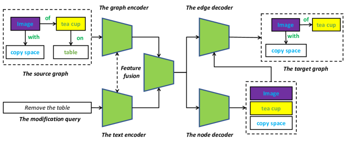
Figure 4: The information flow of our model. Green boxes denote the main computational units.

3.2.1 Graph Encoder: Sparsely Connected Transformer

The standard transformer architecture Vaswani et al. (2017); Yang et al. (2019) relies on a grid of fully-connected self-attention to obtain the contextualized representations from a sequence of elements. In this work, we propose the graph-conditioned, sparsely connected transformer to encode the information from a graph. Our idea is partially inspired by the sparse transformer through factorization Child et al. (2019). Despite the similar name, the two methods share very few similarities in both motivations and mechanisms. The architecture of our graph encoder with the sparely connected transformer is detailed below.

Compared to natural language text, graphs are structured data, which are comprised of two main components: nodes and edges. To efficiently encode a graph, we need to encode the information not only from these constituent components, but also their interactions, namely the node-edge association and connectivity. Thus, we incorporate the information from all the edges to the nodes from which these edges are originated. More formally, our edge-aware node embedding $\boldsymbol{\mathbf{x}}_{i}$ can be obtained from the list of source graph nodes and edges via,

$$\boldsymbol{\mathbf{x}}_{i}=\boldsymbol{\mathbf{T}}^{\mathcal{N}}[x_{i}]+\sum_{j\in J(i)}\boldsymbol{\mathbf{T}}^{\mathcal{E}}[x_{ij}],\vspace{-2mm}$$ (4)

where $\boldsymbol{\mathbf{T}}^{\mathcal{N}}$ and $\boldsymbol{\mathbf{T}}^{\mathcal{E}}$ are the embedding tables for node and edge labels respectively, and $J(i)$ is the set of nodes connected (both inbound and outbound) to the $i$th node in the graph.

After getting the edge-aware node embeddings, we employ the sparsely connected transformer to learn the contextualized embeddings of the whole graph. Unlike the conventional transformer, we do not incorporate the positional encoding into our graph inputs because the nodes are not in a predetermined sequence. Given the edge information from $\boldsymbol{\mathbf{x}}^{\mathcal{E}}$, we enforce the connectivity information by making nodes only visible to its first order neighbor. Let us denote the attention grid of the transformer as A. We then define $A[\boldsymbol{\mathbf{x}}_{i},\boldsymbol{\mathbf{x}}_{j}]=f(\boldsymbol{\mathbf{x}}_{i},\boldsymbol{\mathbf{x}}_{j})$ if $x_{i,j}\in\boldsymbol{\mathbf{x}}^{\mathcal{E}}$ or zero otherwise, where $f$ denotes the normalized inner product function.

The sparsely connected transformer, thus, provides the graph node representations which are conditioned on the graph structure, using the edge labels in the input embeddings and sparse layers in self-attention. We denote the node representations in the output of the sparsely connected transformer by $[\boldsymbol{\mathbf{m}}_{x_{1}},..,\boldsymbol{\mathbf{m}}_{x_{|\boldsymbol{\mathbf{x}}^{\mathcal{N}}|}}]$.

3.2.2 Query Encoder

We use a standard transformer encoder Vaswani et al. (2017) to encode the modification query $\boldsymbol{\mathbf{y}}=(y_{1},..,y_{|\boldsymbol{\mathbf{y}}|})$ into $[\boldsymbol{\mathbf{m}}_{y_{1}},...,\boldsymbol{\mathbf{m}}_{y_{|\boldsymbol{\mathbf{y}}|}}]$. Crucially, in order to encourage semantic alignment, we share the parameters of the graph and query encoders.

3.2.3 Information Fusion of Encoders

In a conventional encoder-decoder model, usually there is only one encoder. In our scenario, there are two sources of information, which require separate encoders. The most straightforward way to incorporate the two information sources is through concatenation. Concretely, the combined representation would be,

$$\boldsymbol{\mathbf{m}}=[\boldsymbol{\mathbf{m}}_{x_{1}},...,\boldsymbol{\mathbf{m}}_{x_{|\boldsymbol{\mathbf{x}}^{\mathcal{V}}|}},\boldsymbol{\mathbf{m}}_{y_{1}},...,\boldsymbol{\mathbf{m}}_{y_{|\boldsymbol{\mathbf{y}}|}}].$$ (5)

The decoder component will then be responsible for information communication between the two encoders through its connections to them. In the following, we propose more advanced methods to combine the two sources of information.

Late Fusion via Gating.

To enhance the ability of the model to combine the encoders’ information for a better use of the decoder, we introduce a parametric approach with the gating mechanism. Through the gating mechanism, we aim to filter useful information from the graph based on the modification query, and vice versa.

More specifically, we add a special [CLS] token to the graph and in front of the query sentence. The representation of this token in the encoders will then capture the holistic understanding, which we denote by $\boldsymbol{\mathbf{m}}_{\boldsymbol{\mathbf{x}}^{\mathcal{G}}}$ and $\boldsymbol{\mathbf{m}}_{\boldsymbol{\mathbf{y}}}$ for the graph and modification query respectively. We make use of these holistic meaning vectors to filter useful information from the representations of the graph nodes $\boldsymbol{\mathbf{m}}_{x_{i}}$ and modification query tokens $\boldsymbol{\mathbf{m}}_{y_{j}}$ as follows,

$$\boldsymbol{\mathbf{g}}_{x_{i}} \!\!\!=\!\!\! \boldsymbol{\sigma}(\mathrm{MLP}(\boldsymbol{\mathbf{m}}_{x_{i}},\boldsymbol{\mathbf{m}}_{\boldsymbol{\mathbf{y}}}))$$ (6)

$$\boldsymbol{\mathbf{m}}^{\prime}_{x_{i}} \!\!\!=\!\!\! \boldsymbol{\mathbf{g}}_{x_{i}}\odot\boldsymbol{\mathbf{m}}_{x_{i}}$$ (7)

$$\boldsymbol{\mathbf{g}}_{y_{j}} \!\!\!=\!\!\! \boldsymbol{\sigma}(\mathrm{MLP}(\boldsymbol{\mathbf{m}}_{y_{j}},\boldsymbol{\mathbf{m}}_{\boldsymbol{\mathbf{x}}^{\mathcal{G}}}))$$ (8)

$$\boldsymbol{\mathbf{m}}^{\prime}_{y_{j}} \!\!\!=\!\!\! \boldsymbol{\mathbf{g}}_{y_{j}}\odot\boldsymbol{\mathbf{m}}_{y_{j}},$$ (9)

where $\mathrm{MLP}$ is a multi-layer perceptron, $\odot$ indicates an element-wise multiplication, and $\boldsymbol{\sigma}$ is the element-wise sigmoid function used to construct the gates $\boldsymbol{\mathbf{g}}_{x_{i}}$ and $\boldsymbol{\mathbf{g}}_{y_{j}}$. The updated node $\boldsymbol{\mathbf{m}}^{\prime}_{x_{i}}$ and token $\boldsymbol{\mathbf{m}}^{\prime}_{y_{j}}$ are then used in the joint encoders representation of Equation 5.

We refer to this gating mechanism as late fusion since it does not let the information from the graph and text interact in their respective lower level encoders. In other words, the fusion happens after the contextualized information has already been learned.

Early Fusion via Cross-Attention.

To allow a deeper interaction between the graph and text encoders, we explore fusing features at the early stage before the contextualized node $\boldsymbol{\mathbf{m}}_{x_{i}}$ and token $\boldsymbol{\mathbf{m}}_{y_{i}}$ representations are learned. This is achieved via cross-attention, an early fusion technique.

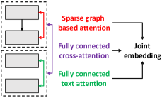
Figure 5: Cross-attention fusion.

Recall that the parameters of the graph and query encoders are shared to enable encoding of the two sources in the same semantic space. That is, we use the same transformer encoder for both sources. In cross-attention, we concatenate the $\boldsymbol{\mathbf{x}}$ (from Equation 4) and $\boldsymbol{\mathbf{y}}$ before rather than after the transformer encoder. As such, the encoder’s input is $[\boldsymbol{\mathbf{x}},\boldsymbol{\mathbf{y}}]$. In the transformer, the representation of each query token gets updated by self-attending to the representations of all the query tokens and graph nodes in the previous layer. However, the representation of each graph node gets updated by self-attending only to its graph neighbors according to the connections of the sparsely connected transformer as well as all query tokens. The final representation $\boldsymbol{\mathbf{m}}$ is taken from the output of transformer. Figure 5 shows the information flow in the cross-attention mechanism.

3.2.4 Node-level Decoder

We use GRU cells Cho et al. (2014) for our RNN decoders. The node-level decoder is a vanilla auto-regressive model described as,

$$\boldsymbol{\mathbf{h}}^{\mathcal{N}}_{t}=\mathrm{GRU}^{\mathcal{N}}(z_{t-1},\boldsymbol{\mathbf{h}}^{\mathcal{N}}_{t-1})$$ (10)

$$\boldsymbol{\mathbf{c}}^{\mathcal{N}}_{t}=\mathrm{ATTN}^{\mathcal{N}}(\boldsymbol{\mathbf{h}}^{\mathcal{N}}_{t},\boldsymbol{\mathbf{m}})$$ (11)

$$p(z_{t}\mid\boldsymbol{\mathbf{z}}_{<t},\boldsymbol{\mathbf{x}}^{\mathcal{G}},\boldsymbol{\mathbf{y}})=$$ (12)

$$\quad\quad\quad\quad\quad\mathrm{softmax}(\boldsymbol{\mathbf{W}}[\boldsymbol{\mathbf{h}}^{\mathcal{N}}_{t},\boldsymbol{\mathbf{c}}^{\mathcal{N}}_{t}]+\boldsymbol{\mathbf{b}}),$$ (13)

where $\boldsymbol{\mathbf{z}}_{<t}$ denotes the nodes generated before time step $t$, $\mathrm{ATTN}^{\mathcal{N}}$ is a Luong-style attention Luong et al. (2015), and $\boldsymbol{\mathbf{m}}$ is the memory vectors from information fusion of the encoders (see §3.2.3).

3.2.5 Edge-level Decoder

For the edge decoder, we first use an adjacency-style generation You et al. (2018). The rows/columns of the adjacency matrix are labeled by the nodes in the order that they have been generated by the node-level decoder. For each row, we have an auto-regressive decoder which emits the label of each edge to other nodes from the edge vocabulary, including a special token [NULL] showing an edge does not exist. As shown in Figure 6, we are only interested in the lower-triangle part of the matrix, as we assume that the node decoder has generated the nodes in a topologically sorted manner. The dashed upper-triangle part of the adjacency matrix are used only for parallel computation, and they will be discarded.

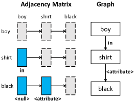
Figure 6: Adjacency matrix style decoder.

We use an attentional decoder using GRU units for generating edges. It operates similarly to the node-level decoder using Equation 11 and Equation 12. For more accurate typed edge generation, however, we incorporate the hidden states of the source and target nodes (from the node decoder) as inputs when updating the hidden state of the edge decoder:

$$\boldsymbol{\mathbf{h}}^{\mathcal{E}}_{i,j} \!\!\!=\!\!\! \mathrm{GRU}^{\mathcal{E}}(z_{i,j-1},\boldsymbol{\mathbf{h}}^{\mathcal{N}}_{i},\boldsymbol{\mathbf{h}}^{\mathcal{N}}_{j},\boldsymbol{\mathbf{h}}^{\mathcal{E}}_{i,j-1}),$$ (14)

where $\boldsymbol{\mathbf{h}}^{\mathcal{E}}_{i,j}$ is the hidden state of the edge decoder for row $i$ and column $j$, and $z_{i,j-1}$ is the label of the previously generated edge from node $i$ to $j-1$.

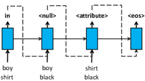
Figure 7: A flat edge-level decoder.

However, there are two drawbacks in this edge generation method. Firstly, the dummy edges in the adjacency matrix cause a waste of computation. Secondly, the edges generated by the previous rows are not conditioned upon when the edges in the next row are generated. However, it may be beneficial to use the information about the outgoing edges of the previous nodes to enhance the generation accuracy of the outgoing edges of the next node. We will analyze this hypothesis in §4. Hence, we suggest flattening the lower-triangle of the adjacency matrix. We remove the dummy edges and concatenate the rows of the lower triangular matrix to form a sequence of pairs of nodes for which we need to generate edges (Figure 7). This strategy results in using information about all previously generated edges when a new edge is generated.

	Synthetic Data			User-Generated Data
	Edge F1	Node F1	Graph Acc	Edge F1	Node F1	Graph Acc
Baselines
Copy Source	64.62	78.41	-	31.42	66.17	-
Text2Text	72.74	91.47	64.42	52.68	78.59	52.15
Modified GraphRNN You et al. (2018)	55.76	80.64	50.72	57.17	80.68	56.75
Graph Transformer Cai and Lam (2019)	75.68	91.21	71.38	59.43	81.47	58.23
DCGCN Guo et al. (2019)	72.47	89.08	68.89	54.23	79.05	52.67
Our Models
Fully Conn Trans + Adj Matrix + Concat	76.49*	91.54	72.13*	57.47	81.29	56.91
Sparse Trans + Adj Matrix + Concat	77.94*	91.94	74.68*	57.78	81.36	56.98
Sparse Trans + Flat-Edge + Concat	79.13*	92.11	76.13*	57.92	81.74	57.03
Sparse Trans + Flat-Edge + Gating	80.13*	92.54*	77.04*	59.58*	82.39*	59.63*
Sparse Trans + Flat-Edge + Cross-Attn	86.52*	95.40*	82.97*	62.10*	83.69*	60.90*

Table 1: Node-level, edge-level and graph-level matching score (%) over two datasets (modified from MSCOCO). “*” indicates statistically significant difference (p <0.0001) from the best baseline.

4 Experiments

Baselines.

We consider five baselines for comparison. In “Copy Source” baseline (i), the system copies the source graph to the target graph. In the “Text2Text” baseline (ii), we flatten the graph and reconstruct the natural sentence similarly to the modification query. In the “Modified GraphRNN” baseline (iii), we use the breadth-first-search (BFS) based node ordering to flatten the graph, and use RNNs as the encoders You et al. (2018) and a decoder similar to our systems. In the final two baselines, “Graph Transformer” (iv) and “Deep Convolutional Graph Networks” (DCGCN) (v), we use the Graph Transformers Cai and Lam (2019) and Deep Convolutional Graph Networks Guo et al. (2019) to encode the source graph (the decoder is identical to ours).

Our Model Configurations.

We report the results of different configurations of our model. The “Fully Connected Transformer” uses dense connections for the graph encoder. This is in contrast to “Sparse Transformer”, which uses the connectivity structure of the source graph in self attention (see §3.2.1). The information from the graph and query encoders can be combined by “Concatenation”, late fused by “Gating”, or early fused by “Cross Attention” (see §3.2.3). The “Adjacency Matrix” style for edge decoding can be replaced with “Flat-Edge” generation (see §3.2.5).

Evaluation Metrics.

We use two automatic metrics for the evaluation. Firstly, we calculate the precision/recall/F1-score of the generated nodes and edges. Secondly, we use the strict-match accuracy, which requires the generated graph to be identical to the target graph for a correct prediction.

Data Splits.

We partition the synthetic MSCOCO data into 196K/2K/2K for training/dev/test, and GCC data into 400K/7K/7K for training/dev/test. We randomly split the crowdsourced user-generated data into 30K/1K/1K for training/dev/test.

4.1 Experimental Results

Table 1 reports the results of our model and the baselines on the synthetic and user-generated datasets. From the experimental results, various configurations of our model are superior to the baselines by a significant margin. Noticeably, DCGCN and graph transformer are strong baselines, delivering SOTA performance across tasks such as AMR-to-text generation and syntax-based neural machine translation Guo et al. (2019); Cai and Lam (2019). We believe the larger number of edge types in our task impairs their capability.

We ablate the different components of the proposed methods to appraise their effectiveness (c.f., the bottom pane of table 1). First, our hypothesis about the preference of flat-edge generation over adjacency matrix-style edge generation is confirmed. Furthermore, the two-way communication between the graph and query encoders through the gating mechanism consistently outperforms a simple concatenation in terms of both edge-level and node-level generation. Eventually the cross-attention – the early fusion mechanism, leads to substantial improvement in all metrics.

We also observe that generating the graphs for the crowdsourced data is much harder than the synthetic data, which we believe is caused by diversity in semantics and expressions introduced by the annotators. Consequently, all models suffer from performance degradation.

	MSCOCO			GCC
	Edge F1	Node F1	Graph Acc	Edge F1	Node F1	Graph Acc
Graph Trans.	75.68	91.21	71.38	42.76	82.38	34.31
Concat	79.13	92.11	76.13	45.09	86.93	37.53
Gating	80.13	92.54	77.04	52.85	91.60	45.79
Cross-Attn	86.52	95.40	82.97	57.68	93.84	52.50

Table 2: Node/Edge/Graph level matching scores comparing the best baseline - Graph Transformer to our model variants on synthetic MSCOCO and GCC.

	MOPs (avg. 1.44)			MOPs (avg. 2.01)
	1-2	3-4	5+	1-2	3-4	5+
Text2Text	27.40	0.87	0.00	26.84	2.38	0.24
M. GraphRNN	26.10	0.64	0.00	25.17	1.81	0.00
Graph Trans.	29.97	1.75	0.00	29.14	4.26	0.53
Cross-Attn	47.95	14.82	1.01	49.93	19.77	4.45

Table 3: Graph-level accuracy on two multiple operations (MOPs) datasets, one with an average of 1.44 operations per query, the other with 2.01

Nevertheless, the performance trends of different configurations of our model are almost identical on the user-generated and synthetic data. Finally, Table 2 indicates with the increase of the complexity of graphs, the models have a difficulty in inferring the relations among nodes for GCC data, which causes a dramatic drop in terms of the edge F1 score and graph accuracy.

4.2 Multi-Operation Performance

To study the multiple operations scenario, we create two datasets where the average number of the operations are 1.44 and 2.01. For each dataset, we train the baselines and our methods on the full training set. The test set is grouped into four bins according to the number of operations.

According to Table 3, all models demonstrate sharp decreases in performance with the increase of the number of operations. Our model still performs significantly better than the baselines. Having said that, for more than 1-2 operations, all models do not perform satisfactorily, prompting further research.

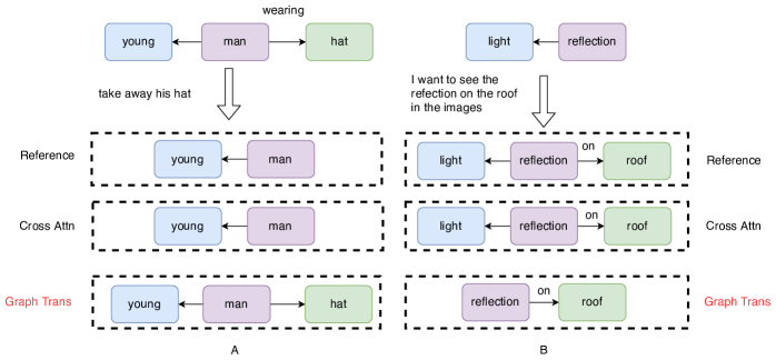
Figure 8: Our best model vs the Graph Transformer.

4.3 Quantitative Analysis

The best configuration of our model is based on cross-attention, with flat-edge decoder, and sparse transformer. We investigate which cases this configuration outperforms the baselines. As seen in Figure 8, cross-attention is able to understand the pronoun and correctly removes the connected object and its associated relation as evidenced by the first example A. In addition, example B demonstrates when graph transformer observes a longer description, it lacks the capability of fusing the semantics between the source graph and the modification query; then certain nodes from the source graph are not preserved. We believe that the proposed approach can reduce the noise in graph generation, and retain fine-grained details better than the baselines.

5 Related Work

Semantic parsing is a sequence-to-graph transduction task, mapping natural language sentences to their meaning representation, e.g. see Buys and Blunsom (2017); Iyer et al. (2017); Dong and Lapata (2018); this is different from our graph conditional semantic parsing. Recently, context-dependent semantic parsing has gained attraction Iyyer et al. (2017); Srivastava et al. (2017); Suhr et al. (2018); He et al. (2019). Our work focuses on the update of scene graphs based on users’ queries, while previous works model the modifications of semantic representations in multi-turn dialogue systems. Due to their effectiveness, GCNs and graph transformer have been used as graph encoder for graph-to-sequence transduction in semantic-based text generation Bastings et al. (2017); Beck et al. (2018); Guo et al. (2019); Cai and Lam (2019); Song et al. (2018); Wu et al. (2020).

6 Conclusion

In this paper, we explore a novel problem of conditional graph modification, in which a system needs to modify a source graph according to a modification command. Our best system, which is based on graph-conditioned transformers and cross-attention information fusion, outperforms strong baselines adapted from machine translations and graph generations. The code and datasets will be released to encourage further research in this direction.

Appendix A Training Details

Our encoder is comprised of 3 stacked sparse transformers, with 4 heads at each layer. The embedding size is 256, and the inner-layer of feed-forward networks has a dimension of 512. Both node-level and edge-level decoders are one-layer GRU-RNN with a hidden size of 256, and the size of embeddings are 256 as well. We train 30 epochs and 300 epochs for synthetic and user-generated data respectively, with batch size of 256. We evaluate the model over the dev set every epoch, and choose the checkpoint with the best graph accuracy for the inference. We run all experiments on a single Nvidia Tesla V100.

Table 4 shows that our cross-attention model is more efficient than other models in terms of GPU computing time. Table 5 displays the number of parameters used for each model.

	MSCOCO		GCC
	syn	crowd.	syn.
DGCN	205	325	712
Graph Trans.	126	114	478
Concat	146	160	457
Gating	248	248	534
Cross-Attn	93	132	469

Table 4: GPU time (ms/step) over different settings at training stage.

	MSCOCO		GCC
	syn	crowd.	syn.
DGCN	10.9M	16.3M	19.3M
Graph Trans.	9.9M	15.2M	18.4M
Concat	8.1M	12.8M	15.4M
Gating	8.1M	12.8M	15.4M
Cross-Attn	8.1M	12.8M	15.4M

Table 5: Number of parameters over different settings.

Appendix B Performance on validation set

Table 6 shows the performance on the validation/dev set of our models and the best baseline. In general, there is no significant difference between the performance trend in the dev set and the test set.

	Synthetic				Crowsourced
	MSCOCO		GCC
	dev	test	dev	test	dev	test
Graph Trans.	72.01	71.38	40.14	34.31	59.88	58.23
Concat	77.34	76.13	43.16	37.53	59.20	57.03
Gating	78.06	77.04	52.87	45.79	60.48	59.63
Cross-Attn.	84.12	82.97	60.21	52.50	61.20	60.90

Table 6: Results of the best baseline and our models on dev and test splits.

Appendix C Data Statistics

As shown in Table 7, the graph size distributions of source graphs and target graphs are almost identical among the sets. With the increase in text description length, the source graphs become more complicated accordingly. According to Figure 9, the length of search queries are likely to be less than 5 tokens. Thus, in a real application, it is unlikely to encounter large graphs (>3 nodes) and long modification queries.

We plot the distributions of the number of nodes and edges on synthetic and user-generated data in Figure 10.

	Synthetic (Train/Dev/Test)		Crowsourced
	MSCOCO	GCC	Train/Dev/Test
size	196k / 2k / 2k	400k / 7k / 7k	30k / 1k / 1k
Ave. #tokens / text desc	5.2 / 5.2 / 5.2	10.1 / 10.1 / 10.2	4.8 / 4.8 / 4.8
Ave. #nodes / src graph	2.9 / 2.9 / 2.9	3.8 / 3.8 / 3.8	2.0 / 2.0 / 2.0
Ave. #edges / src graph	1.9 / 1.9 / 1.9	2.9 / 2.8 / 2.8	1.0 / 1.0 / 1.0
Ave. #nodes / tgt graph	2.9 / 2.9 / 2.8	3.8 / 3.8 / 3.8	2.0 / 2.0 / 2.0
Ave. #edges / tgt graph	1.9 / 1.9 / 1.8	2.9 / 2.8 / 2.8	1.0 / 1.0 / 1.0
Ave. #tokens / src query	4.7 / 4.8 / 4.7	4.9 / 4.8 / 4.9	10.1 / 10.2 / 10.0

Table 7: Statistics of the created datasets.

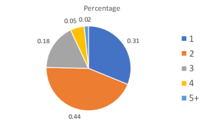
Figure 9: The percentage of the length of queries from in-house search log.

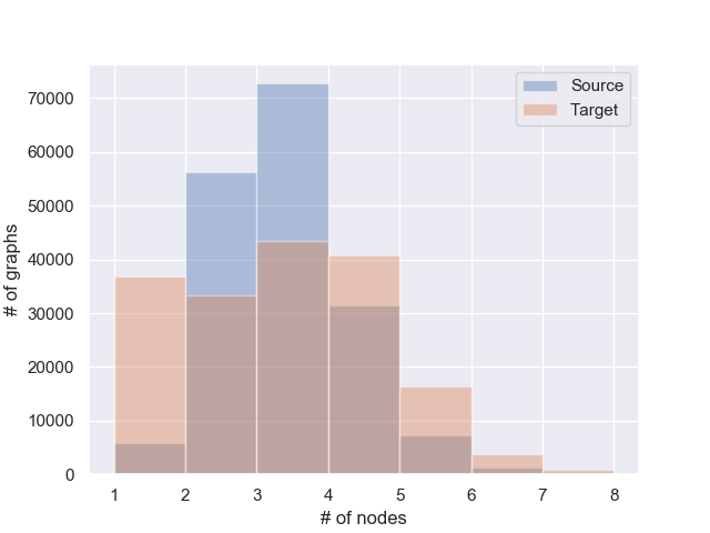
(a) Distribution of nodes on synthetic data

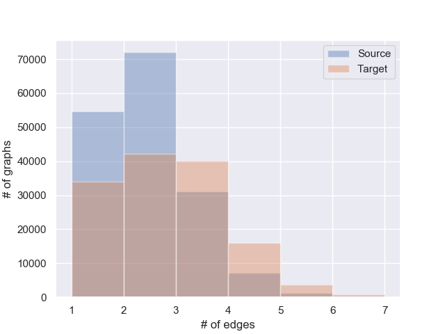
(b) Distribution of edges on synthetic data

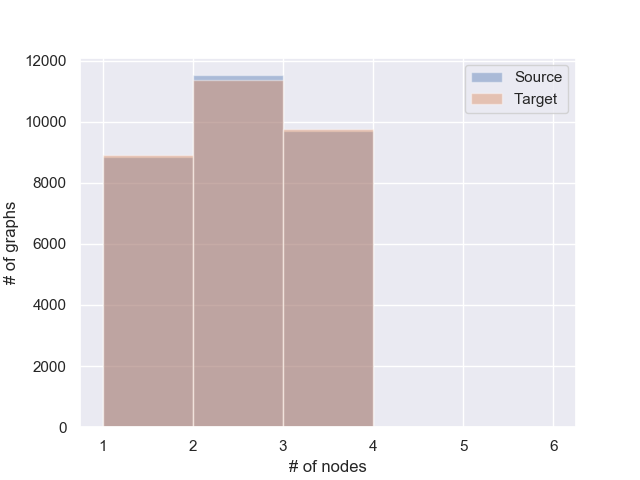
(c) Distribution of nodes on user-generated data

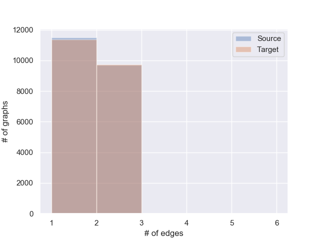
(d) Distribution of edges on user-generated data

Figure 10: The distributions of the number of nodes and edges on synthetic and user-generated data among source graphs and target graphs.

Appendix D Data Creation for Multi-operation Graph Modification

We develop a procedure to create data for the multi-operation graph modification (MGM) task. First of all, we assume that MGM requires at least one operation on the source graph. Then we use four actions (terminate, ins, del, sub) paired with a heuristic algorithm to further perform operations on the modified graph. We sample an action, and execute it on the last modified graph until the terminate is sampled or we exhaust the available nodes. Intuitively, a large graph can support more modifications, while a smaller graph does not have too much freedom. In addition, we also assume that the modified nodes should not be changed again. Hence, the probability of terminate should be increased as the edit sequence gets longer, whereas the probabilities of other actions should drop. The heuristic algorithm is summarized in Algorithm 1. It is worth noting that Algorithm 1 gives us a dataset with different edit sequence lengths.

Algorithm 1 Multiple operations for graph modifications

0:  $G$: scene graphs, $I$: insertion templates, $D$: deletion templates, $S$: substitution templates

0:  $X$: source graphs, $Z$: target graphs, $Y$: modified queries,

1:  $X$ $\leftarrow$ $\{\}$, $Z$ $\leftarrow$ $\{\}$, $Y$ $\leftarrow$ $\{\}$

2:  $A$ $\leftarrow$ $\{ins,del,sub\}$,

3:  for $k=1$ to $|G|$ do

4:     $g$ $\leftarrow$ $G_{k}$

5:     $a$ $\sim$ uniform($A$)

6:     if $a$ == $ins$ then

7:        $s,q,t$ $\leftarrow$ $\mathrm{insertion}(g,I)$

8:     else if $a$ == $del$ then

9:        $s,q,t$ $\leftarrow$ $\mathrm{deletion}(g,D)$

10:     else

11:        $s,q,t$ $\leftarrow$ $\mathrm{substitution}(g,S)$

12:     end if

13:     $A$ $\leftarrow$ $\{terminate,ins,del,sub\}$,

14:     $w$ $\leftarrow$ $\{P,1,1,1\}$, {$P$ controls the average number of operations.}

15:     while True do

16:        total $\leftarrow$ $\mathrm{TotalNode(t)}$

17:        avail $\leftarrow$ $\mathrm{AvailableNode(t)}$

18:        if len(avail) == 0 then

19:           break

20:        end if

21:        $D$ $\leftarrow$ $softmax(w^{\frac{total-avail}{total*\tau}})$

22:        a $\sim$ $sample$($A$, $D$)

23:        if $a$ == $terminate$ then

24:           break

25:        else if $a$ == $ins$ then

26:           $s,q^{\prime},t$ $\leftarrow$ $\mathrm{insertion}(s,t,I)$

27:        else if $a$ == $del$ then

28:           $s,q^{\prime},t$ $\leftarrow$ $\mathrm{deletion}(s,t,D)$

29:        else

30:           $s,q^{\prime},t$ $\leftarrow$ $\mathrm{substitution}(s,t,S)$

31:        end if

32:     end while

33:     $q$ $\leftarrow$ $\mathrm{concat(q,q^{\prime})}$

34:     $X$ $\leftarrow$ $X\cup\{s\}$, $Z$ $\leftarrow$ $Z\cup\{t\}$, $Y$ $\leftarrow$ $Y\cup\{q\}$

35:  end for

36:  return $X$, $Z$, $Y$

Appendix E Mixing Synthetic and User-generated Data

Getting annotation from users is expensive, especially for a complex task like our graph modification problem. Thus, we explore the possibility of augmenting the user-generated data with synthetic data in order to train a better model. However, one needs to be careful with data augmentation using synthetic data as it inevitably has a different distribution. This is evident when we test the model trained using the synthetic data on the user-generated data. The graph generation accuracy drops to around 20%, and adding more synthetic data does not help. To efficiently mix the data distributions, we up-sample the user-generated data and mix it with synthetic data with a ratio of 1:1 in each mini-batch.

We compare data augmentation using upsampling with transfer learning – another method to learn from both synthetic and user-generated data OpenAI et al. (2019). We pretrain our model using the synthetic data, and then fine-tune it on the user-generated data.

Synthetic Data Size	30k	60k	90k	120k	150k
Trained with:
Synthetic only	21.63	19.33	22.03	22.40	18.87
Pretrain-Finetune	61.40	63.37	63.87	62.300	63.47
Data Augment.	70.27	72.37	74.80	74.67	75.23

Table 8: Graph accuracy (%) over different data settings. 30k means adding 30k synthetic instances.

Table 8 reports the results. It shows that data augmentation with up-sampling is a very effective method to leverage both sources of data, compared to transfer learning. Also, as the size of the synthetic data increases, our proposed scheme further improves the performance to a certain point where it plateaus. More specifically, the performance reaches plateau after injecting 90k instances (the data ratio of 3:1). Both up-sampling and pre-training lead to better models compared to using only synthetic or user-generated data. The graph accuracy for model trained only on user-generated data is 60.90% (see the best result from Table 1 in the main paper).

Appendix F Templates

In Table 9, we summarize the templates used for our synthetic data.

Insertion:

I want xx, I prefer xx, I like xx

I would like to see xx, Show me xx,

Give me xx, I’m interested in xx

I need xx, Search for xx, Return xx

(xx are nodes to be inserted)

Deletion:

remove xx, I do not want xx, delete xx

I do not like xx, omit xx, I do not need xx

erase xx, ignore xx, discard xx, drop xx

(xx denotes the node to be deleted)

Substitution:

change xx to yy, update xx to yy

replace xx with yy, substitute yy for xx

I prefer yy to xx, modify xx to yy

I want yy rather than xx, switch xx to yy

convert xx to yy, give me yy instead of xx

(xx and yy are old nodes and updated nodes)

Table 9: Simplified templates for synthetic data, with each operation has 10 templates.

Appendix G Examples from User-generated Dataset

We provides some examples of our user-generated dataset in Figure 11.

Appendix H Alignments between Different Components

Figure 13 and Figure 14 provide the alignments between different components of our cross attention model. Indeed, the cross attention is capable of aligning the source graph to the modification query.

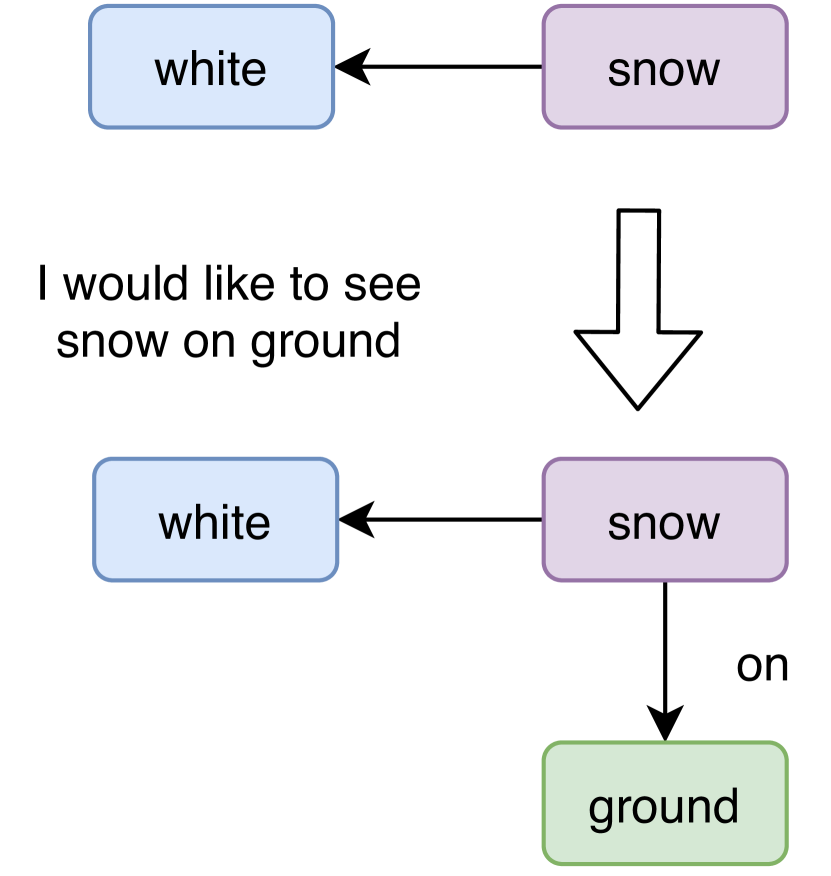
(a) Insertion

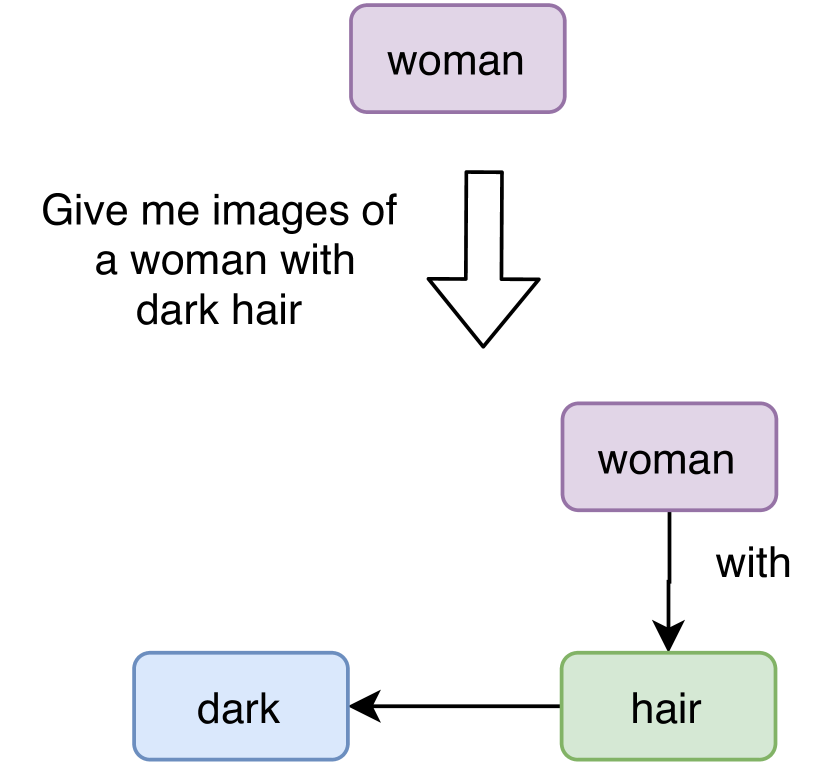
(b) Insertion

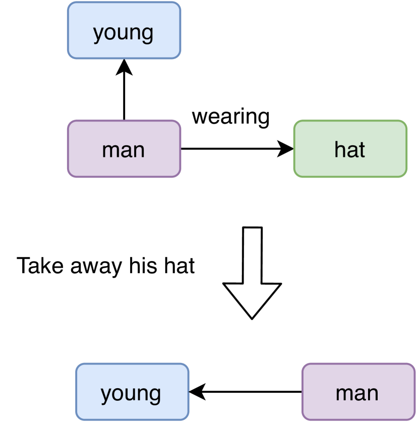
(c) Deletion

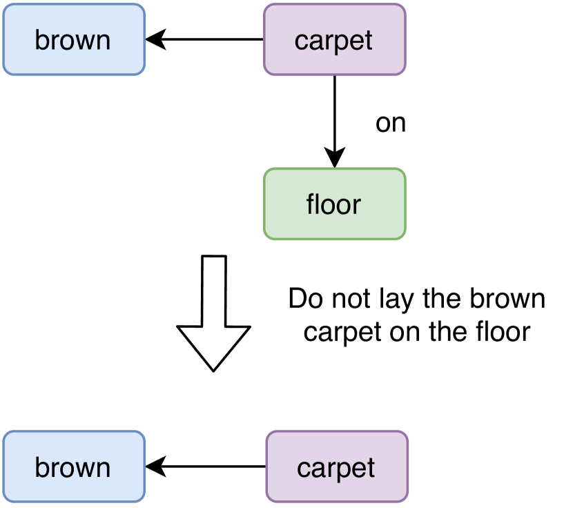
(d) Deletion

Figure 11: Examples from the user-generated dataset.

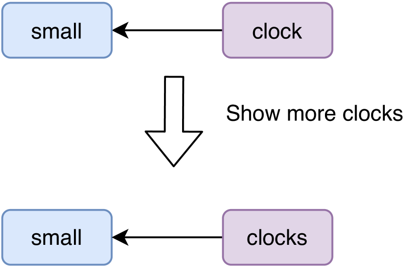
(a) Object substitution

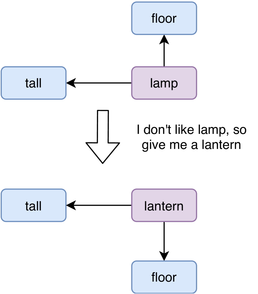
(b) Object substitution

(c) Attribute substitution

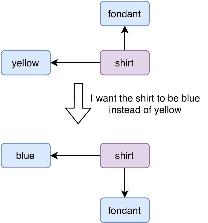
(d) Attribute substitution

Figure 12: Examples from the user-generated dataset.

(a) An example of graph modification

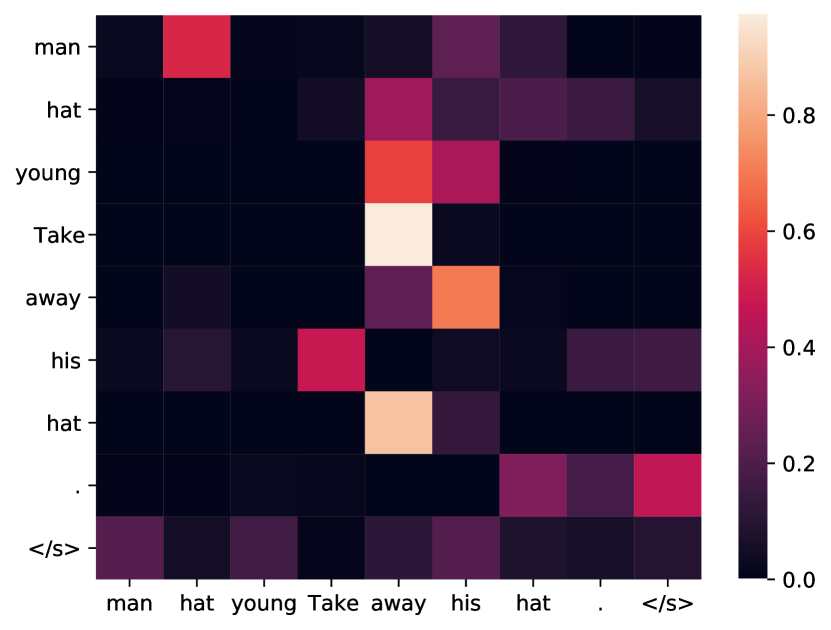
(b) Cross Attention between query and source graph

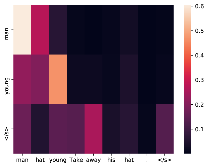
(c) Attention between source information and target nodes

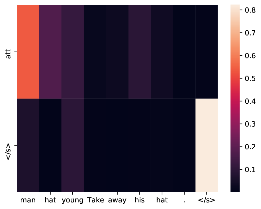
(d) Attention between source information and target edges

Figure 13: Alignments between different components.

(a) An example of graph modification

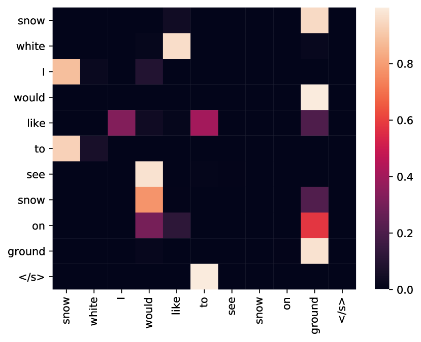
(b) Cross Attention between query and source graph

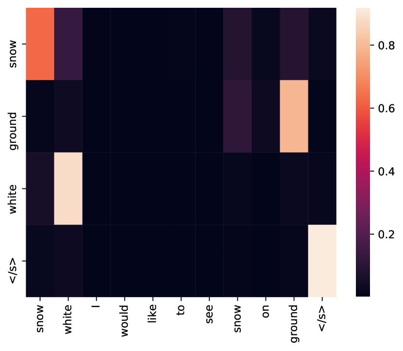
(c) Attention between source information and target nodes

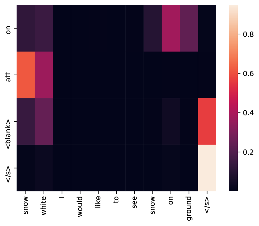
(d) Attention between source information and target edges

Figure 14: Alignments between different components.

References

- Anderson et al. (2016) Peter Anderson, Basura Fernando, Mark Johnson, and Stephen Gould. 2016. Spice: Semantic propositional image caption evaluation. In European Conference on Computer Vision, pages 382–398. Springer.
- Bahdanau et al. (2014) Dzmitry Bahdanau, Kyunghyun Cho, and Yoshua Bengio. 2014. Neural machine translation by jointly learning to align and translate. arXiv preprint arXiv:1409.0473.
- Bastings et al. (2017) Joost Bastings, Ivan Titov, Wilker Aziz, Diego Marcheggiani, and Khalil Sima’an. 2017. Graph convolutional encoders for syntax-aware neural machine translation. In Proceedings of the 2017 Conference on Empirical Methods in Natural Language Processing, pages 1957–1967, Copenhagen, Denmark. Association for Computational Linguistics.
- Beck et al. (2018) Daniel Beck, Gholamreza Haffari, and Trevor Cohn. 2018. Graph-to-sequence learning using gated graph neural networks. In Proceedings of the 56th Annual Meeting of the Association for Computational Linguistics (Volume 1: Long Papers), pages 273–283.
- Buys and Blunsom (2017) Jan Buys and Phil Blunsom. 2017. Robust incremental neural semantic graph parsing. In Proceedings of the 55th Annual Meeting of the Association for Computational Linguistics, pages 1215–1226.
- Cai and Lam (2019) Deng Cai and Wai Lam. 2019. Graph transformer for graph-to-sequence learning. arXiv preprint arXiv:1911.07470.
- Chen and Manning (2014) Danqi Chen and Christopher Manning. 2014. A fast and accurate dependency parser using neural networks. In Proceedings of the 2014 conference on empirical methods in natural language processing (EMNLP), pages 740–750.
- Child et al. (2019) Rewon Child, Scott Gray, Alec Radford, and Ilya Sutskever. 2019. Generating long sequences with sparse transformers. arXiv preprint arXiv:1904.10509.
- Cho et al. (2014) Kyunghyun Cho, Bart van Merriënboer, Caglar Gulcehre, Dzmitry Bahdanau, Fethi Bougares, Holger Schwenk, and Yoshua Bengio. 2014. Learning phrase representations using rnn encoder–decoder for statistical machine translation. In Proceedings of the 2014 Conference on Empirical Methods in Natural Language Processing (EMNLP), pages 1724–1734.
- Clark et al. (2018) Kevin Clark, Minh-Thang Luong, Christopher D Manning, and Quoc Le. 2018. Semi-supervised sequence modeling with cross-view training. In Proceedings of the 2018 Conference on Empirical Methods in Natural Language Processing, pages 1914–1925.
- Dong and Lapata (2018) Li Dong and Mirella Lapata. 2018. Coarse-to-fine decoding for neural semantic parsing. In Proceedings of the 56th Annual Meeting of the Association for Computational Linguistics, pages 731–742.
- Dozat and Manning (2016) Timothy Dozat and Christopher D Manning. 2016. Deep biaffine attention for neural dependency parsing. arXiv preprint arXiv:1611.01734.
- Edunov et al. (2018) Sergey Edunov, Myle Ott, Michael Auli, and David Grangier. 2018. Understanding back-translation at scale. In Proceedings of the 2018 Conference on Empirical Methods in Natural Language Processing, pages 489–500.
- Gardner et al. (2017) Matt Gardner, Joel Grus, Mark Neumann, Oyvind Tafjord, Pradeep Dasigi, Nelson F. Liu, Matthew Peters, Michael Schmitz, and Luke S. Zettlemoyer. 2017. Allennlp: A deep semantic natural language processing platform.
- Guo et al. (2019) Zhijiang Guo, Yan Zhang, Zhiyang Teng, and Wei Lu. 2019. Densely connected graph convolutional networks for graph-to-sequence learning. Transactions of the Association for Computational Linguistics, 7:297–312.
- He et al. (2019) Xuanli He, Quan Hung Tran, and Gholamreza Haffari. 2019. A pointer network architecture for context-dependent semantic parsing. In Proceedings of the The 17th Annual Workshop of the Australasian Language Technology Association, pages 94–99.
- Iyer et al. (2017) Srinivasan Iyer, Ioannis Konstas, Alvin Cheung, Jayant Krishnamurthy, and Luke Zettlemoyer. 2017. Learning a neural semantic parser from user feedback. In Proceedings of the 55th Annual Meeting of the Association for Computational Linguistics, pages 963–973.
- Iyyer et al. (2017) Mohit Iyyer, Wen-tau Yih, and Ming-Wei Chang. 2017. Search-based neural structured learning for sequential question answering. In Proceedings of the 55th Annual Meeting of the Association for Computational Linguistics (Volume 1: Long Papers), pages 1821–1831.
- Jean et al. (2015) Sébastien Jean, Orhan Firat, Kyunghyun Cho, Roland Memisevic, and Yoshua Bengio. 2015. Montreal neural machine translation systems for wmt’15. In Proceedings of the Tenth Workshop on Statistical Machine Translation, pages 134–140.
- Johnson et al. (2015) Justin Johnson, Ranjay Krishna, Michael Stark, Li-Jia Li, David Shamma, Michael Bernstein, and Li Fei-Fei. 2015. Image retrieval using scene graphs. In Proceedings of the IEEE conference on computer vision and pattern recognition, pages 3668–3678.
- Kipf and Welling (2016) Thomas N. Kipf and Max Welling. 2016. Semi-supervised classification with graph convolutional networks. CoRR, abs/1609.02907.
- Krishna et al. (2017) Ranjay Krishna, Yuke Zhu, Oliver Groth, Justin Johnson, Kenji Hata, Joshua Kravitz, Stephanie Chen, Yannis Kalantidis, Li-Jia Li, David A Shamma, et al. 2017. Visual genome: Connecting language and vision using crowdsourced dense image annotations. International Journal of Computer Vision, 123(1):32–73.
- Li et al. (2018) Yujia Li, Oriol Vinyals, Chris Dyer, Razvan Pascanu, and Peter Battaglia. 2018. Learning deep generative models of graphs.
- Lin et al. (2014) Tsung-Yi Lin, Michael Maire, Serge Belongie, James Hays, Pietro Perona, Deva Ramanan, Piotr Dollár, and C Lawrence Zitnick. 2014. Microsoft coco: Common objects in context. In European conference on computer vision, pages 740–755. Springer.
- Luong et al. (2015) Minh-Thang Luong, Hieu Pham, and Christopher D Manning. 2015. Effective approaches to attention-based neural machine translation. In Proceedings of the 2015 Conference on Empirical Methods in Natural Language Processing, pages 1412–1421.
- Manuvinakurike et al. (2018) Ramesh Manuvinakurike, Jacqueline Brixey, Trung Bui, Walter Chang, Doo Soon Kim, Ron Artstein, and Kallirroi Georgila. 2018. Edit me: A corpus and a framework for understanding natural language image editing. In Proceedings of the Eleventh International Conference on Language Resources and Evaluation (LREC 2018).
- Mrini et al. (2019) Khalil Mrini, Franck Dernoncourt, Trung Bui, Walter Chang, and Ndapa Nakashole. 2019. Rethinking self-attention: An interpretable self-attentive encoder-decoder parser. arXiv preprint arXiv:1911.03875.
- OpenAI et al. (2019) OpenAI, Ilge Akkaya, Marcin Andrychowicz, Maciek Chociej, Mateusz Litwin, Bob McGrew, Arthur Petron, Alex Paino, Matthias Plappert, Glenn Powell, Raphael Ribas, Jonas Schneider, Nikolas Tezak, Jerry Tworek, Peter Welinder, Lilian Weng, Qiming Yuan, Wojciech Zaremba, and Lei Zhang. 2019. Solving rubik’s cube with a robot hand.
- Perez and Liu (2017) Julien Perez and Fei Liu. 2017. Dialog state tracking, a machine reading approach using memory network. In Proceedings of the 15th Conference of the European Chapter of the Association for Computational Linguistics: Volume 1, Long Papers, pages 305–314.
- Ren et al. (2018) Liliang Ren, Kaige Xie, Lu Chen, and Kai Yu. 2018. Towards universal dialogue state tracking. In Proceedings of the 2018 Conference on Empirical Methods in Natural Language Processing, pages 2780–2786.
- Schuster et al. (2015) Sebastian Schuster, Ranjay Krishna, Angel Chang, Li Fei-Fei, and Christopher D Manning. 2015. Generating semantically precise scene graphs from textual descriptions for improved image retrieval. In Proceedings of the fourth workshop on vision and language, pages 70–80.
- Sharma et al. (2018) Piyush Sharma, Nan Ding, Sebastian Goodman, and Radu Soricut. 2018. Conceptual captions: A cleaned, hypernymed, image alt-text dataset for automatic image captioning. In Proceedings of the 56th Annual Meeting of the Association for Computational Linguistics (Volume 1: Long Papers), pages 2556–2565, Melbourne, Australia. Association for Computational Linguistics.
- Simonovsky and Komodakis (2018) Martin Simonovsky and Nikos Komodakis. 2018. Graphvae: Towards generation of small graphs using variational autoencoders. In International Conference on Artificial Neural Networks, pages 412–422. Springer.
- Song et al. (2018) Linfeng Song, Yue Zhang, Zhiguo Wang, and Daniel Gildea. 2018. A graph-to-sequence model for amr-to-text generation. In Proceedings of the 56th Annual Meeting of the Association for Computational Linguistics (Volume 1: Long Papers), pages 1616–1626.
- Srivastava et al. (2017) Shashank Srivastava, Amos Azaria, and Tom M Mitchell. 2017. Parsing natural language conversations using contextual cues. In IJCAI, pages 4089–4095.
- Suhr et al. (2018) Alane Suhr, Srinivasan Iyer, and Yoav Artzi. 2018. Learning to map context-dependent sentences to executable formal queries. In Proceedings of the 2018 Conference of the North American Chapter of the Association for Computational Linguistics: Human Language Technologies, Volume 1 (Long Papers), pages 2238–2249.
- Vaswani et al. (2017) Ashish Vaswani, Noam Shazeer, Niki Parmar, Jakob Uszkoreit, Llion Jones, Aidan N Gomez, Łukasz Kaiser, and Illia Polosukhin. 2017. Attention is all you need. In Advances in neural information processing systems, pages 5998–6008.
- Vendrov et al. (2015) Ivan Vendrov, Ryan Kiros, Sanja Fidler, and Raquel Urtasun. 2015. Order-embeddings of images and language. arXiv preprint arXiv:1511.06361.
- Wang et al. (2018) Yu-Siang Wang, Chenxi Liu, Xiaohui Zeng, and Alan Yuille. 2018. Scene graph parsing as dependency parsing. In Proceedings of the 2018 Conference of the North American Chapter of the Association for Computational Linguistics: Human Language Technologies, Volume 1 (Long Papers), pages 397–407.
- Wu et al. (2020) Zonghan Wu, Shirui Pan, Fengwen Chen, Guodong Long, Chengqi Zhang, and S Yu Philip. 2020. A comprehensive survey on graph neural networks. IEEE Transactions on Neural Networks and Learning Systems.
- Yang et al. (2019) Xu Yang, Kaihua Tang, Hanwang Zhang, and Jianfei Cai. 2019. Auto-encoding scene graphs for image captioning. In Proceedings of the IEEE Conference on Computer Vision and Pattern Recognition, pages 10685–10694.
- You et al. (2018) Jiaxuan You, Rex Ying, Xiang Ren, William L Hamilton, and Jure Leskovec. 2018. Graphrnn: Generating realistic graphs with deep auto-regressive models. arXiv preprint arXiv:1802.08773.
- Zhou and Zhao (2019) Junru Zhou and Hai Zhao. 2019. Head-driven phrase structure grammar parsing on penn treebank. In Proceedings of the 57th Annual Meeting of the Association for Computational Linguistics, pages 2396–2408.