Dissecting Span Identification Tasks with Performance Prediction

Abstract

Span identification (in short, span ID) tasks such as chunking, NER, or code-switching detection, ask models to identify and classify relevant spans in a text. Despite being a staple of NLP, and sharing a common structure, there is little insight on how these tasks’ properties influence their difficulty, and thus little guidance on what model families work well on span ID tasks, and why. We analyze span ID tasks via performance prediction, estimating how well neural architectures do on different tasks.

Our contributions are: (a) we identify key properties of span ID tasks that can inform performance prediction; (b) we carry out a large-scale experiment on English data, building a model to predict performance for unseen span ID tasks that can support architecture choices; (c), we investigate the parameters of the meta model, yielding new insights on how model and task properties interact to affect span ID performance. We find, e.g., that span frequency is especially important for LSTMs, and that CRFs help when spans are infrequent and boundaries non-distinctive.

1 Introduction

Span identification is a family of analysis tasks that make up a substantial portion of applied NLP. Span identification (or short, span ID) tasks have in common that they identify and classify contiguous spans of tokens within a running text. Examples are named entity recognition (Nadeau and Sekine, 2007), chunking (Tjong Kim Sang and Buchholz, 2000), entity extraction (Etzioni et al., 2005), quotation detection (Pareti, 2016), keyphrase detection (Augenstein et al., 2017), or code switching (Pratapa et al., 2018). In terms of complexity, span ID tasks form a middle ground between simpler analysis tasks that predict labels for single linguistic units (such as lemmatization Porter (1980) or sentiment polarity classification Liu (2012)) and more complex analysis tasks such as relation extraction, which combines span ID with relation identification (Zelenko et al., 2002; Adel et al., 2018).

Due to the rapid development of deep learning, an abundance of model architectures is available for the implementation of span ID tasks. These include isolated token classification models Berger et al. (1996); Chieu and Ng (2003), probabilistic models such as hidden Markov models Rabiner (1989), maximum entropy Markov models McCallum et al. (2000), and conditional random fields Lafferty et al. (2001), recurrent neural networks such as LSTMs Hochreiter and Schmidhuber (1997), and transformers such as BERT Devlin et al. (2019).

Though we have some understanding what each of these models can and cannot learn, there is, to our knowledge, little work on systematically understanding how different span ID tasks compare: are there model architectures that work well generally? Can we identify properties of span ID tasks that can help us select suitable model architectures on a task-by-task basis? Answers to these questions could narrow the scope of architecture search for these tasks, and could help with comparisons between existing methods and more recent developments.

In this work, we address these questions by applying meta-learning to span identification (Vilalta and Drissi, 2002; Vanschoren, 2018). Meta-learning means “systematically observing how different machine learning approaches perform […] to learn new tasks much faster” (Vanschoren, 2018), with examples such as architecture search (Elsken et al., 2019) and hyperparameter optimization (Bergstra and Bengio, 2012). Our specific approach is to apply performance prediction for span ID tasks, using both task properties and model architectures as features, in order to obtain a better understanding of the differences among span ID tasks.

Concretely, we collect a set of English span ID tasks, quantify key properties of the tasks (such as how distinct the spans are from their context, and how clearly their boundaries are marked) and formulate hypotheses linking properties to performance (Section 2). Next, we describe relevant neural model architectures for span ID (Section 3). We then train a linear regressor as a meta-model to predict span ID performance based on model features and task metrics in an unseen-task setting (Section 4). We find the best of these architectures perform at or close to the state of the art, and their success can be relatively well predicted by the meta-model (Section 5). Finally, we carry out a detailed analysis of the regression model’s parameters (Section 6), gaining insight into the relationship between span ID tasks and different neural model architectures. For example, we establish that spans that are not very distinct from their context are consistently difficult to identify, but that CRFs are specifically helpful for this class of span ID tasks.

2 Datasets, Span Types, and Hypotheses

We work with five widely used English span ID datasets. All of them have non-overlapping spans from a closed set of span types. In the following, we discuss (properties of) span types, assuming that each span type maps onto one span ID task.

2.1 Datasets

Quotation Detection: parc and RiQuA.

The Penn Attribution Relation Corpus (parc) version 3.0 (Pareti, 2016) and the Rich Quotation Attribution Corpus (RiQuA, Papay and Padó, 2020) are two datasets for quotation detection: models must identify direct and indirect quotation spans in text, which can be useful for social network construction Elson et al. (2010) and coreference resolution Almeida et al. (2014). The corpora cover articles from the Penn Treebank (parc) and 19th century English novels (RiQuA), respectively. Within each text, quotations are identified, along with each quotation’s speaker (or source), and its cue (an introducing word, usually a verb like “said”). We model detection of quotations as well as cues. As speaker and addressee identification are relation extraction tasks, we exclude these span types.

Chunking: CoNLL’00.

Chunking (shallow parsing) is an important preprocessing step in a number of NLP applications. We use the corpus from the 2000 CoNLL shared task on chunking (CoNLL’00) (Tjong Kim Sang and Buchholz, 2000). Like parc, this corpus consists of a subset of the PTB. This dataset is labeled with non-overlapping chunks of eleven phrase types. In our study, we consider the seven phrase types with $>$100 instances in the training partition: ‘ADJP’, ‘ADVP’, ‘NP’, ‘PP’, ‘PRT’, ‘SBAR’, and ‘VP’.

NER: OntoNotes and ChemDNer.

For recognition and classification of proper names, we use the NER layer of OntoNotes Corpus v5.0 (Weischedel et al., 2013) and Biocreative’s ChemDNer corpus v1.0 (Krallinger et al., 2015). OntoNotes, a general language NER corpus, is our largest dataset, with over 2.2 million tokens. The NER layer comprises 18 span types, both typical entity types such as ‘Person’ and ‘Organization’ as well as numerical value types such as ‘Date’ and ‘Quantity’. We use all span types. ChemDNer is a NER corpus specific to chemical and drug names, comprising titles and abstracts from 10000 PubMed articles. It labels names of chemicals and drugs and assigns them to eight classes, corresponding to chemical name nomenclatures. We use seven span types: ‘Abbreviation’, ‘Family’, ‘Formula’, ‘Identifier’, ‘Systematic’, ‘Trivial’, and ‘Multiple’. We exclude the class ‘No class’ as infrequent ($<$100 instances).

2.2 Span Type Properties and Hypotheses

While quotation detection, chunking, and named entity recognition are all span ID tasks, they vary quite widely in their properties. As mentioned in the introduction, we know of little work on quantifying the similarities and differences of span types, and thus, span ID tasks.

Task	Dataset	freq	len	SD	BD
Quotation	parc	16480	7.89	1.34	1.43
Quotation	RiQuA	4026	9.84	1.46	1.57
Chunking	CoNLL’00	37168	1.55	1.26	0.64
NER	ChemDNer	6110	1.62	3.08	0.96
NER	OntoNotes	16861	1.63	3.36	1.00

Table 1: Span type metrics (values averaged over all span types in each corpus, weighted by span type frequency, computed on training sets). SD = span distinctiveness, BD = boundary distinctiveness. Values for individual span types can be found in Table 7 in the Appendix.

We now present four metrics which we propose to capture the relevant characteristics of span types, and make concrete our hypotheses regarding their effect on model performance. Table 1 reports frequency-weighted averages for each metric on each dataset. See Table 7 in the Appendix for all span-type-specific values.

Frequency is the number of spans for a span type in the dataset’s training corpus. It is well established that the performance of a machine learning model benefits from higher amounts of training data (Halevy et al., 2009). Thus, we expect this property to be positively correlated with performance. However, some architectural choices, such as the use of transfer learning, are purported to reduce the data requirements of machine learning models (Pan and Yang, 2009), so we expect a smaller correlation for architectures which incorporate transfer learning.

Span length is the geometric mean of spans’ lengths, in tokens. Scheible et al. (2016) note that traditional CRF models perform poorly at the identification of long spans due to the strict Markov assumption they make Lafferty et al. (2001). Thus, we expect architectures which rely on such assumptions and which have no way to model long distance dependencies to perform poorly on span types with a high average span length, while LSTMs or transformers should do better on long spans (Khandelwal et al., 2018; Vaswani et al., 2017).

Span distinctiveness is a measure of how distinctive the text that comprises spans is compared to the overall text of the corpus. Formally, we define it as the KL divergence $D_{\text{KL}}(P_{\text{span}}||P)$, where $P$ is the unigram word distribution of the corpus, and $P_{\text{span}}$ is the unigram distribution of tokens within a span. A high span distinctiveness indicates that different words are used inside spans compared to the rest of the text, while a low span distinctiveness indicates that the word distribution is similar inside and outside of spans.

We expect this property to be positively correlated with model performance. Furthermore, we hypothesize that span types with a high span distinctiveness should be able to rely more heavily on local features, as each token carries strong information about span membership, while low span distinctiveness calls for sequence information. Consequently, we expect that architectures incorporating sequence models such as CRFs, LSTMs, and transformers should perform better at low-distinctive span types.

Boundary distinctiveness is a measure of how distinctive the starts and ends of spans are. We formalize this in terms of a KL-divergence as well, namely as $D_{\text{KL}}(P_{\text{boundary}}||P)$ between the unigram word distribution ($P$) and the distribution of boundary tokens ($P_{\text{boundary}}$), where boundary tokens are those which occur immediately before the start of a span, or immediately after the end of a span. A high boundary distinctiveness indicates that the start and end points of spans are easy to spot, while low distinctiveness indicates smooth transitions.

We expect boundary distinctiveness to be positively correlated with model performance, based on studies that obtained improvements from specifically modeling the transition between span and context Todorovic et al. (2008); Scheible et al. (2016). As sequence information is required to utilize boundary information, high boundary distinctiveness should improve performance more for LSTMs, CRFs, or transformers.

Task Profiles.

As Table 1 shows, the metrics we propose appear to capture the task structure of the datasets well: quotation corpora have long spans with low span distinctiveness (anything can be said) but high boundary distinctiveness (punctuation, cues). Chunking has notably low boundary distinctiveness, due to the syntactic nature of the span types, and NER spans show high distinctiveness (semantic classes) but are short and have somewhat indistinct boundaries as well.

3 Model Architectures

For span identification, we use the BIO framework (Ramshaw and Marcus, 1999), framing span identification as a sequence labeling task. As each span type has its own B and I labels, and there is one O label, a dataset with $n$ span types leads to a $2n+1$-label classification problem for each token.

We investigate a set of sequence labeling models, ranging from baselines to state-of-the-art architectures. We group our models by common components, and build complex models through combination of simpler models. Except for the models using BERT, all architectures assume one 300-dimensional GloVe embedding (Pennington et al., 2014) per token as input.

Baseline.

As a baseline model, we use a simple token-level classifier. This architecture labels each token using a softmax classifier without access to sequence information (neither at the label level nor at the feature level).

CRF.

This model uses a linear-chain conditional random field (CRF) to predict token label sequences (Lafferty et al., 2001). It can access neighboring labels in the sequence of predictions.

LSTM and LSTM+CRF.

These architectures incorporate Bi-directional LSTMs (biLSTMs) (Hochreiter and Schmidhuber, 1997; Schuster and Paliwal, 1997) as components. The simplest architecture, LSTM, passes the inputs through a 2-layer biLSTM network, and then predicts token labels using a softmax layer. The LSTM+CRF architecture combines the biLSTM network with a CRF layer, training all weights simultaneously. These models can learn to combine sequential input and labeling information.

BERT and BERT+CRF.

These architectures include the pre-trained BERT language model (Devlin et al., 2019) as a component. The simplest architecture in this category, BERT, comprises a pre-trained BERT encoder and a softmax output layer, which is trained while the BERT encoder is fine-tuned. BERT+CRF combines a BERT encoder with a linear-chain CRF output layer, which directly uses BERT’s output embeddings as inputs. In this architecture, the CRF layer is first trained to convergence while BERT’s weights are held constant, and then both models are jointly fine-tuned to convergence. As BERT uses WordPiece tokenization (Wu et al., 2016), the input must be re-tokenized for BERT architectures.

BERT+LSTM+CRF.

This architecture combines all components previously mentioned. It first uses a pre-trained BERT encoder to generate a sequence of contextualized embeddings. These embeddings are projected to 300 dimensions using a linear layer, yielding a sequence of vectors, which are then used as input for a LSTM+CRF network. As with BERT+CRF, we first train the non-BERT parameters to convergence while holding BERT’s parameters fixed, and subsequently fine-tune all parameters jointly.

Handcrafted Features.

Some studies have shown marked increases in performance by adding hand-crafted features (e.g. Shimaoka et al., 2017). We develop such features for our tasks and treat these to be an additional architecture component. For architectures with this component, a bag of features is extracted for each token (the exact features used for each dataset are enumerated in Table 5 in the Appendix). For each feature, we learn a 300-dimensional feature embedding which is averaged with the GloVe or BERT embedding to obtain a token embedding. Handcrafted features can be used with the Baseline, LSTM, LSTM+CRF, and BERT+LSTM+CRF architectures. BERT and BERT+CRF cannot utilize manual features, as they have no way of accepting token embeddings as input.

4 Meta-learning Model

Recall that our meta-learning model is a model for predicting the performance of the model architectures from Section 3 when applied to span identification tasks from Section 2. We model this task of performance prediction as linear regression, a well established framework for the statistical analysis of language data (Baayen, 2008). The predictors are task properties, model architecture properties, and their interactions, and the dependent variable is (scaled) $F_{1}$ score.

While a linear model is not powerful enough to capture the full range of interactions, its weights are immediately interpretable, it can be trained on limited amounts of data, and it does not overfit easily (see Section 5.1). All three properties make it a reasonable choice for meta-learning.

Predictors and Interactions.

As predictors for our performance prediction task, we use the span type properties described above, and a number of binary model properties. For the span type properties [freq] and [span length], we use the logarithms of these values as predictors. The two distinctiveness properties are already logarithms, and so we used them as-is. For model properties, we used four binary predicates: The presence of handcrafted features, of a CRF output layer, of a bi-LSTM layer, and of a BERT layer.

In addition to main effects of properties of models and corpora on performance (does a CRF layer help?), we are also interested in interactions of these properties (does a CRF layer help in particular for longer spans?). As such interactions are not captured automatically in a linear regression model, we encode them as predictors. We include interactions between span type and model properties, as well as among model properties.

All predictors (including interactions) are standardized so as to have a mean of zero and standard deviation of one.

Scaling the Predicted Performance

Instead of directly predicting the $F_{1}$ score, we instead make our predictions in a logarithmic space, which eases the linearity requirements of linear regression. We cannot directly use the logit function to transform $F_{1}$ scores into $F^{\prime}=\text{logit}\left(\frac{F_{1}}{100}\right)$ since the presence of zeros in our $F_{1}$ scores makes this process ill-defined. Instead, we opted for a “padded” logit transformation $F^{\prime}=\text{logit}\left((1-\alpha)\cdot\frac{F_{1}}{100}+\alpha\cdot\frac{100-F_{1}}{100}\right)$ with a hyperparameter $\alpha\in\left[0,0.5\right)$. This rescales the argument of the logit function from $[0,1]$ to the smaller interval $[\alpha,1-\alpha]$, avoiding the zero problem of a bare logit. Through cross-validation (cf. Section 5.1), we set $\alpha=0.2$. We use the inverse of this transformation to scale the output of our prediction as an $F_{1}$ score, clamping the result to $[0,100]$.

5 Experiment

5.1 Experimental Procedure

	BL	Feat BL	CRF	Feat CRF	LSTM	Feat LSTM	LSTM CRF	Feat LSTM CRF	BERT	BERT CRF	BERT LSTM CRF	BERT Feat LSTM CRF
parc	34.8	31.4	46.6	57.9	64.8	76.9	76.0	81.8	78.7	81.4	82.4	82.5
RiQuA	21.7	14.5	19.7	14.4	67.5	76.7	79.6	81.7	79.8	82.5	82.1	82.3
CoNLL’00	55.9	60.0	79.7	87.1	87.7	92.3	90.0	93.5	96.3	96.5	96.6	96.6
OntoNotes	39.0	27.4	61.2	67.7	58.8	65.1	76.4	84.7	85.9	86.8	86.5	87.5
ChemDNer	49.8	19.6	56.9	58.5	57.0	45.7	71.2	75.1	83.3	84.7	84.9	84.8

Table 2: Average architecture results on datasets. BL=Baseline, Feat=Hand-crafted features. For each dataset, we micro-average performance over all span types, and average these micro-averages across five trials. For comparability with existing work, we include all span types in these micro-averages, even those which we exclude from our performance prediction. Full performance results for each span type can be found in Table 8.

Our meta learning experiment comprises two steps: Span ID model training, and meta model training.

Step 1: Span ID model training.

We train and subsequently evaluate each model architecture on each dataset five times, using different random initializations. With 12 model architectures and 5 datasets under consideration, this procedure yields $12\times 5\times 5=300$ individual experiments.

For each dataset, we use the established train/test partition. Since RiQuA does not come with such a partition, we use cross-validation, partitioning the dataset by its six authors and holding out one author per cross-validation step.

We use early stopping for regularization, stopping training once (micro-averaged) performance on a validation set reaches its maximum. To prevent overfitting, all models utilize feature dropout – during training, each feature in a token’s bag of input features is dropped with a probability of 50%. At evaluation time, all features are used.

Step 2: Meta learning model training.

This step involves training our performance prediction model on the $F_{1}$ scores obtained from the first step. For each architecture-span-type pair of the 12 model architectures and 36 span types, we already obtained 5 $F_{1}$ scores. This yields a total of $12\times 36\times 5=2160$ input-output pairs to train our performance prediction model.

We investigate both $L^{1}$ and $L^{2}$ regularization in an elastic net setting (Zou and Hastie, 2005) but consistently find best cross-validation performance with no regularization whatsoever. Thus, we use ordinary least squares regression.

To ensure that our performance predictions generalize, we use a cross-validation setup when generating model predictions. To generate performance predictions for a particular span type, we train our meta-model on data from all other span types, holding out the span type for which we want a prediction. We repeat this for all 36 span types, holding out a different span type each time, in order to collect performance predictions for each span type.

5.2 Span Identification Results

Step 1 yields 5 evaluation $F_{1}$ scores for each architecture–span-type pair. This section summarizes the main findings. Detailed average scores for each pair are reported in Table 8 in the Appendix.

Table 2 lists the micro-averaged performance of each model architecture on each dataset. Unsurprisingly, BERT+Feat+LSTM+CRF, the model with the most components, performs best on three of the five datasets. This provides strong evidence that this architecture can perform well across many tasks. However, note that architecture’s dominance is somewhat overstated by only looking at average dataset results. Our analysis permits us to look more closely at results for individual span types, where we find that BERT+Feat+LSTM+CRF performs best on 16 of the 36 total span types, BERT+CRF on 7 span types, Feat+LSTM+CRF on 7 span types, and BERT+LSTM+CRF on 6 span types. Thus, ‘bespoke’ modeling of span types can evidently improve results.

Even though our architectures are task-agnostic, and not tuned to particular tasks or datasets, our best architectures still perform quite competitively. For instance, on CoNLL’00, our BERT+Feat+LSTM+CRF model comes within 0.12 $F_{1}$ points of the best published model’s $F_{1}$ score of 97.62 (Akbik et al., 2018). For parc, existing literature does not report micro-averaged $F_{1}$ scores, but instead focuses only on $F_{1}$ scores for content span detection. In this case, we find that our BERT+Feat+LSTM+CRF model beats the existing state of the art on this span type, achieving an $F_{1}$ score of 78.1, compared to the score of 75 reported in Scheible et al. (2016).

5.3 Meta-learning Results

	MAE	$r^{2}$
Full model	11.38	0.73
No interactions	14.00	0.61
Only architecture predictors	18.88	0.37
Only task predictors	20.87	0.22
Empty model	23.78	N/A

Table 3: Evaluation of performance prediction models

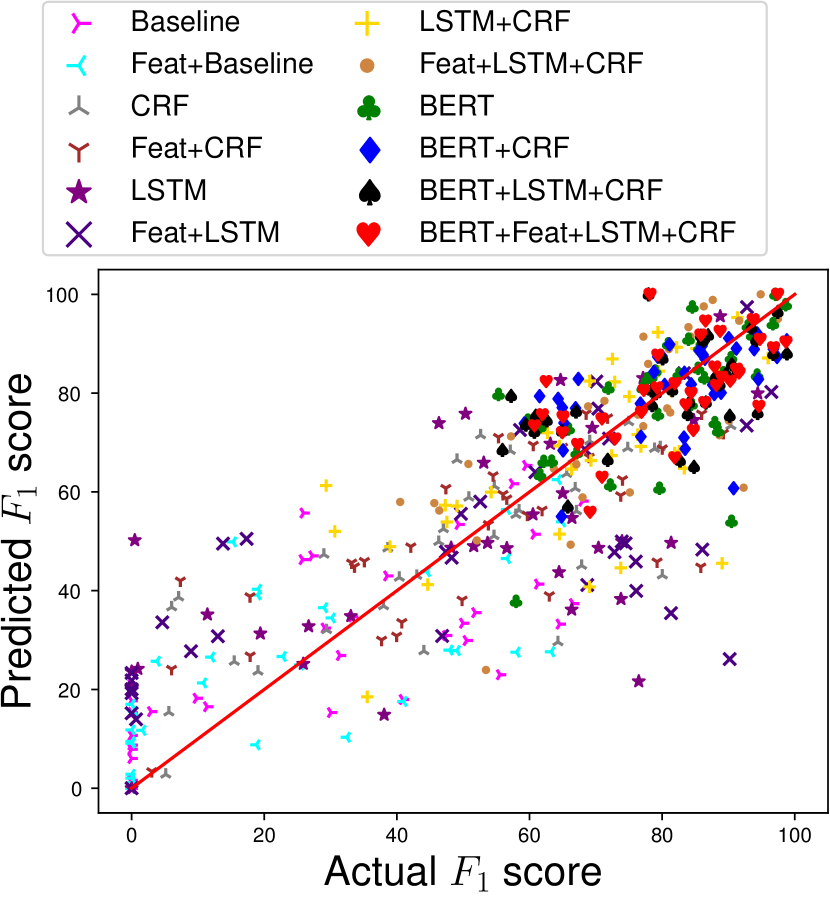
Figure 1: Scatterplot of actual vs. predicted $F_{1}$ scores for all 36 span types $\times$ 12 model architectures

The result of Step 2 is our performance prediction model. Table 3 shows both mean absolute error (MAE), which is directly interpretable as the mean difference between predicted and actual F₁ score for each data point, and $r^{2}$, which provides the amount of variance accounted for by the model. The full performance prediction model, including both span type and model architecture features, accounts for 73% of the variance, with an MAE of about 11. We see this as an acceptable model fit. To validate the usefulness of the predictor groups and interaction terms, we carry out ablation experiments wherein these are excluded, including a model with no interaction terms, a model with only span type-predictors, a model with only architecture predictors, and an empty model, which only predicts the average of all F₁ scores. The reduced models do better than the empty model, but show marked increases in MAE and corresponding drops in $r^{2}$ compared to the full model. While the usefulness of the architecture predictors is expected, this also constitutes strong evidence for the usefulness of the span type predictors we have proposed in Section 2.

Figure 1 shows a scatterplot of predicted and actual $F_{1}$ scores. Our meta learning model generally predicts high performances better than low performances. The largest cluster of errors occurs for experiments with an actual $F_{1}$ score of exactly zero, arguably an uninteresting case. Thus, we believe that the overall MAE underestimates rather than overestimates the quality of the performance prediction for practical purposes.

6 Analysis

We now investigate the linear regression coefficients of our performance prediction model to assess our hypotheses from Section 2. To obtain a single model to analyze, we retrain our regression model on all data points, with no cross-validation.

Table 4 shows the resulting coefficients. Using Bonferroni correction at $\alpha=0.05$, we consider a coefficient significant if p$<$0.002. Non-significant coefficients are shown in parentheses. Due to the scaling of $F_{1}$ scores performed as described in section 4, the coefficients cannot be directly interpreted in terms of linear change on the $F_{1}$ scale. However, as we standardized all predictors, we can compare coefficients with one another. Coefficients with a greater magnitude have larger effects on $F_{1}$ score, with positive values indicating an increase, and negative values a decrease.

When analyzing these coefficients, one must consider main effects and interactions together. E.g., the main effect coefficient for LSTMs is negative, which seems to imply that adding an LSTM will hurt performance. However, the LSTM $\times$ [freq] and LSTM $\times$ [boundary distinctness] interactions are both strongly positive, so LSTMs should help on frequent span types with high boundary distinctiveness. Our main observations are the following:

Model predictors
Handcrafted		($-$0.11)
CRF		0.50
LSTM		$-$0.35
BERT		1.00
Span type predictors
freq		0.40
length		$-$0.49
span distinct.		$-$0.22
boundary distinct.		0.16
Model–span type interactions
Handcrafted $\times$	freq	(0.05)
	length	($-$0.04)
	span distinct.	($-$0.09)
	boundary distinct.	(0.09)
CRF $\times$	freq	$-$0.33
	length	0.19
	span distinct.	0.34
	boundary distinct.	$-$0.30
LSTM $\times$	freq	0.47
	length	0.08
	span distinct.	($-$0.09)
	boundary distinct.	0.22
BERT $\times$	freq	$-$0.43
	length	0.13
	span distinct.	(0.04)
	boundary distinct.	($-$0.05)
Model–model interactions
Handcrafted $\times$	CRF	0.10
	LSTM	0.05
	BERT	$-$0.05
CRF $\times$	LSTM	($-$0.05)
	BERT	$-$0.24
LSTM $\times$	BERT	$-$0.17

Table 4: Regression coefficients from performance prediction model. Coefficients not statistically significant at $p<0.002$ (as per Bonferroni correction) in parentheses.

Frequency helps, length hurts.

The main effects of our span type predictors show mostly an expected pattern. Frequency has a strong positive effect (frequent span types are easier to learn), while length has an even stronger negative effect (long span types are difficult). More distinct boundaries help performance as well. More surprising is the negative sign of the span distinctiveness predictor, which would mean that more distinct spans are more difficult to recognize. However, this might be due to the negative correlation between span distinctiveness and frequency ($r=-0.46$ in standardized predictors) – less frequent spans are, by virtue of their rarity, more distinctive.

BERT is good for performance, especially with few examples.

The presence of a BERT component is the highest-impact positive predictor for model performance, with a positive coefficient of 1. This finding is not entirely surprising, given the recent popularity of BERT-based models for span identification problems Li et al. (2020); Hu et al. (2019). Furthermore, the strong negative value of the (BERT $\times$ [freq]) predictor shows that BERT’s benefits are strongest when there are few training examples, validating our hypothesis about transfer learning. BERT is also robust: largely independent of span or boundary distinctiveness effects.

LSTMs require a lot of data.

While the main effect of LSTMs is negative, this effect is again modulated by the high positive coefficient of the (LSTM $\times$ [freq]) interaction. This means that their performance is highly dependent on the amount of training data. Also, LSTMs lead to improvements for long span types and those with distinct boundaries – properties that LSTMs arguably can pick up well but that other models struggle with.

CRFs help.

After BERT, the presence of a CRF shows the second-most positive main effect on model performance. Given the strong correlation between adjacent tags in a BIO label sequence, it makes sense that a model capable of enforcing correlations in its output sequence would perform well. CRFs can also exploit span distinctiveness well, presumably by the same mechanism. Surprisingly, CRFs show reduced effectiveness for highly frequent spans with distinct boundaries. We believe that this pattern is best considered as a relative statement: for frequent, well-separated span types CRFs gain less than other model types.

Handcrafted features do not matter much.

We find neither a significant main effect of handcrafted features, nor any significant interactions with span type predictors. Interactions with model predictors are significant, but rather small. While a detailed analysis of architecture-wise $F_{1}$-scores does show that some architectures, such as pure CRFs, do seem to benefit more from hand-crafted features (see Table 8 in the Appendix), this effect diminishes considerably when model components are mixed.

Combining model components shows diminishing returns.

All interactions between LSTM, CRF, and BERT are negative. This demonstrates an overlap in these components’ utility. Thus, a simple “maximal” combination does not always perform best, as Table 2 confirms.

7 Related Work

Meta-learning and performance prediction are umbrella terms which comprise a variety of approaches and formalisms in the literature. We focus on the literature most relevant to our work and discuss the relationship.

Performance Prediction for Trained Models.

In NLP, a number of studies investigate predicting the performance of models that have been trained previously on novel input. An example is Chen (2009) which develops a general method to predict the performance of a family of language models. Similar ideas have been applied more recently to machine translation (Bojar et al., 2017), and automatic speech recognition Elloumi et al. (2018), among others. While these approaches share our goal of performance prediction, they predict performance for the same task and model on new data, while we generalize across tasks and architectures. Thus, these approaches are better suited to estimating confidence at prediction time, while our meta-learning approach can predict a model’s performance before it is trained.

AutoML.

Automated machine learning, or AutoML, aims at automating various aspects of machine learning model creation, including hyperparameter selection, architecture search, and feature engineering (Yao et al., 2018; He et al., 2019) While the task of performance prediction does not directly fall within this research area, a model for predicting performance is directly applicable to architecture search. Within AutoML, the auto-sklearn system (Feurer et al., 2015) takes an approach rather similar to ours, wherein they identify meta-features of datasets, and select appropriate model architectures based on those meta-features. However, auto-sklearn does not predict absolute performance as we do, but instead simply selects good candidate architectures via a $k$-nearest-neighbors approach in meta-feature space. Other related approaches in AutoML use Bayesian optimization, including the combined model selection and hyperparameter optimization of Auto-WEKA (Thornton et al., 2013) and the neural architecture search of Auto-keras (Jin et al., 2019).

Model Interpretability.

A number of works have investigated how to analyze and explain the decisions made by machine learning models. LIME (Mishra et al., 2017) and Anchors (Ribeiro et al., 2018) are examples of systems for explaining a model’s decisions for specific training instances. Other works seek to explain and summarize how models perform across an entire dataset. This can be achieved e.g. through comparison of architecture performances, as in Nguyen and Guo (2007), or through meta-modeling of trained models, as was done in Weiss et al. (2018). Our present work falls into this category, including both a comparison of architectures across datasets and a meta-learning task of model performance.

Meta-learning for One- and Few-shot Learning.

A recent trend is the application of meta-learning to models for one- or few-shot learning. In this setting, a meta-learning approach is used to train models on many distinct tasks, such that they can subsequently be rapidly fine-tuned to a particular task Finn et al. (2017); Santoro et al. (2016). While such approaches use the same meta-learning framework as we do, their task and methodology are substantially different. They focus on learning with very few training examples, while we focus on optimizing performance with normally sized corpora. Additionally, these models selectively train preselected model architectures, while we are concerned with comparisons between architectures.

Model and Corpus Comparisons in Survey Papers.

In a broad sense, our goal of comparison between existing corpora and modeling approaches is shared with many existing survey papers. Surveys include quantitative comparisons of existing systems’ performances on common tasks, producing a results matrix very similar to ours (Li et al., 2020; Yadav and Bethard, 2018; Bostan and Klinger, 2018, i.a.). However, most of these surveys limit themselves to collecting results across models and datasets without performing a detailed quantitative analysis of these results to identify recurring patterns, as we do with our performance prediction approach.

8 Conclusion

In this work, we considered the class of span identification tasks. This class contains a number of widely used NLP tasks, but no comprehensive analysis beyond the level of individual tasks is available. We took a meta-learning perspective, predicting the performance of various architectures on various span ID tasks in an unseen-task setup. Using a number of ‘key metrics’ that we developed to characterize the span ID tasks, a simple linear regression model was able to do so at a reasonable accuracy. Notably, even though BERT-based architectures expectedly perform very well, we find that different variants are optimal for different tasks. We explain such patterns by interpreting the parameters of the regression model, which yields insights into how the properties of span ID tasks interact with properties of neural model architectures. Such patterns can be used for manual fine-grained model selection, but our meta-learning model could also be incorporated directly into AutoML systems.

Our current study could be extended in various directions. First, the approach could apply the same meta-learning approach to other classes of tasks beyond span ID. Second, a larger range of span type metrics could presumably improve model fit, albeit at the cost of interpretability. Third, we only predict within-corpus performance, and corpus-level similarity metrics could be added to make predictions about performance in transfer learning.

Appendix A Training Models

All code used for training span identification and performance prediction models is available for download at our project website: https://www.ims.uni-stuttgart.de/data/span-id-meta-learning. All text logs generated during training of span identification models are included.

A.1 Hardware

All span identification models were trained using GeForce GTX 1080 Ti GPUs. Training time varied considerably across architectures – exact training times for individual experiments are found in the corresponding training logs.

The performance prediction model was trained on a CPU in a few seconds.

parc	Token POS tag
	Token lemma
	Constituents containing token
	Constituents starting at token
	Constituents ending at token
RiQuA	Token POS tag †
	Token lemma †
	Is token a quotation mark?
	Is token a quotation mark?
	Is token capitalized?
	Is token all caps?
CoNLL’00	Token POS tag †
OntoNotes	Token POS tag
	Is token capitalized?
	Is token all caps?
	Character bi- and trigrams
	Constituents containing token
	Constituents starting at token
	Constituents ending at token
ChemDNer	Token POS tag †
	Token lemma †
	Is token capitalized?
	Is token all caps?
	Is token purely alphabetic?
	Is token all digits?

Table 5: Hand-crafted features used. Entries marked with a dagger† were predicted using spaCy (Honnibal and Montani, 2017) – others were either manually annotated, or were exactly specified by the tokens’ surface forms

A.2 Tokenization

For parc, OntoNotes, and CoNLL’00, which include tokenization information, and we use the datasets’ tokenizations directly For RiQuA, we use spaCy (Honnibal and Montani, 2017) to word-tokenize the text. We found that spaCy’s tokenization performed particularly poorly for ChemDNer, and so for this corpus we treated all sequences of alphabetic characters as a token, all sequences of numbers as a token, and all other characters as single-character tokens. For ChemDNer, we found that some spans within the corpus still did not align with token boundaries. In these cases, we excluded the spans entirely from the training data, and treated them as an automatic false-negative for evaluation purposes.

For models including a BERT component, tokens were sub-tokenized using word-piece tokenization (Wu et al., 2016) so as to be compatible with BERT. The same bag of token features was given to each word piece. Models predicted BIO sequences for these sub-tokens, and spans were only evaluated as correct when their boundaries matched exactly with the originally-tokenized corpus.

A.3 Hyperparameters

Hyperparameter	Value
Input dimensionality	300
LSTM units	300
Softmax output layer units	300
CRF units	300
LSTM layers	2
LSTM dropout probability	0.5
Learning rate (non-BERT)	$1\times 10^{-3}$
Learning rate (BERT)	$2\times 10^{-5}$

Table 6: Hyperparameter choices

Due to the large number of experiments run, it was infeasible to do a full grid-search for hyperparameters for each architecture-dataset combination. As such, we tried to pick reasonable values for hyperparameters, motivated by existing literature, prior research, and implementation defaults of existing libraries. For BERT-based models, our choice of pre-trained model – ‘bert-base-uncased’ as provided by the HuggingFace Transformers library Wolf et al. (2019) – fixed some of these hyperparameters for us. Table 6 enumerates the hyperparameter values used for our architectures.

A.4 Optimizer and Training

All models were trained with the Adam optimizer (Kingma and Ba, 2014). For BERT+CRF and BERT+LSTM+CRF, we train the non-BERT parameters as a first training phase, and then fine-tune all parameters jointly as a second training phase. In these cases, Adam was re-initialized between two training phases. For training all non-BERT architectures, and for first training phase in the BERT+CRF and BERT+LSTM+CRF architectures, an initial learning rate of 0.001 was used. For BERT, and for the second training phase in the BERT+CRF and BERT+LSTM+CRF architectures, an initial learning rate of $2\times 10^{-5}$ was used.

A.5 Early Stopping

To guide early stopping, micro-averaged $F_{1}$ scores on the development set were computed after every epoch. These were computed for all span types, including those which were subsequently excluded from our meta-model. For datasets which had no dedicated development partition, a portion of the training set was held out for this purpose. After each epoch, model parameters were saved to disk if the development-set $F_{1}$ score exceeded the best seen so far. An exponential moving average of these $F_{1}$ scores was kept, and training terminated when an epoch’s $F_{1}$ score fell below this average. For BERT+CRF and BERT+LSTM+CRF, this same early stopping procedure was used for both training phases. The training logs list development set performance at each epoch for each experiment.

A.6 Features

Table 5 lists all manual features that were used in models with the “Feat” component.

Appendix B Full Tables

Table 7 lists the span type properties of all span types from all datasets. Table 8 shows average $F_{1}$ score for each combination of span type and model architecture.

Dataset	Span type	Frequency	Span length	Span dist.	Boundary dist.
ChemDNer	Abbreviation	4536	1.17	3.85	0.94
	Family	4089	1.44	3.15	0.99
	Formula	4445	1.98	2.50	0.99
	Identifier	672	2.59	3.61	1.43
	Multiple	202	6.49	2.10	1.60
	Systematic	6654	2.17	2.14	0.98
	Trivial	8832	1.15	3.64	0.86
CoNLL’00	ADJP	2060	1.22	3.13	1.22
	ADVP	4227	1.07	3.02	0.74
	NP	55048	1.89	0.48	0.65
	PP	21281	1.01	2.08	0.59
	PRT	556	1.00	4.59	2.20
	SBAR	2207	1.02	3.68	1.26
	VP	21467	1.39	1.60	0.50
OntoNotes	Cardinal	10901	1.20	3.45	0.90
	Date	18791	1.87	2.62	0.88
	Event	1009	2.65	3.15	1.32
	Facility	1158	2.33	3.54	1.22
	GPE	21938	1.16	3.66	0.81
	Language	355	1.03	7.26	1.99
	Law	459	2.92	3.16	1.69
	Location	2160	1.69	4.14	1.10
	Money	5217	2.61	3.87	1.41
	NORP	9341	1.04	4.85	0.98
	Ordinal	2195	1.00	5.99	1.39
	Organization	24163	1.93	2.22	0.74
	Percent	3802	2.30	4.35	1.50
	Person	22035	1.51	3.54	1.24
	Product	992	1.51	4.58	1.65
	Quantity	1240	2.25	3.79	1.35
	Time	1703	1.95	3.50	1.24
	Work of art	1279	2.77	2.15	1.67
parc	Content	17416	13.86	0.15	1.73
	Cue	15424	1.16	2.69	1.09
RiQuA	Cue	2325	1.05	4.04	1.37
	Quotation	4843	14.06	0.22	1.67

Table 7: A listing of all span types considered for each dataset, along with their frequency, geometric mean span length, span distinctiveness, and boundary distinctiveness.

		Baseline	Feat+Baseline	CRF	Feat+CRF	LSTM	Feat+LSTM	LSTM+CRF	Feat+LSTM+CRF	BERT	BERT+CRF	BERT+LSTM+CRF	BERT+Feat+LSTM+CRF
parc	Content	0.0	1.6	15.5	40.0	50.3	70.4	69.1	77.2	71.7	76.6	77.8	78.1
	Cue	68.0	64.9	69.1	68.5	77.1	83.3	82.2	86.3	84.4	85.8	86.7	86.4
RiQuA	Cue	64.6	49.0	58.4	47.4	73.9	74.5	81.9	80.8	78.8	83.1	83.9	84.3
	Quotation	0.0	0.0	5.6	6.0	76.5	90.2	89.0	92.3	90.3	90.6	90.0	90.2
CoNLL’00	ADJP	29.1	22.8	47.0	61.9	56.6	72.8	66.3	77.2	82.4	84.2	83.6	83.5
	ADVP	51.8	58.0	66.9	74.0	70.4	76.0	76.8	81.2	85.3	86.2	86.4	86.3
	NP	59.5	64.3	79.7	86.0	88.8	92.8	91.4	94.9	97.0	97.1	97.2	97.3
	PP	57.5	56.6	90.4	94.5	94.4	96.5	96.0	97.4	98.5	98.6	98.6	98.6
	PRT	40.9	41.0	64.3	63.0	66.4	68.7	73.8	75.1	84.3	83.3	84.6	84.6
	SBAR	33.2	63.3	67.1	73.8	81.4	86.1	67.1	65.1	94.2	94.3	94.2	94.5
	VP	49.3	56.6	74.8	89.2	84.8	92.7	88.6	94.4	96.6	96.6	96.5	96.7
OntoNotes	Cardinal	25.8	19.0	57.1	55.3	53.1	60.9	72.8	81.0	80.8	80.9	79.9	79.2
	Date	38.6	29.0	65.6	69.0	63.1	68.3	79.5	84.3	85.5	85.9	85.9	85.7
	Event	0.0	0.0	29.4	40.7	0.9	0.0	39.0	46.4	63.2	65.0	60.5	64.9
	Facility	0.0	0.0	7.1	17.8	0.0	0.0	30.6	45.6	62.0	64.7	64.7	72.8
	GPE	60.8	44.5	75.0	76.7	69.5	72.0	85.2	91.6	93.4	94.1	94.0	94.7
	Language	0.0	0.0	29.0	33.2	0.0	0.0	47.5	40.5	72.0	76.5	71.6	70.8
	Law	0.0	0.0	19.1	17.9	0.0	0.0	44.7	52.1	61.5	64.8	55.7	67.2
	Location	11.4	0.0	38.6	42.1	19.4	9.0	54.2	67.1	65.8	67.1	66.8	70.8
	Money	9.8	32.5	67.9	79.2	64.5	76.1	82.6	90.1	87.8	88.7	89.4	88.9
	NORP	66.6	48.0	78.9	80.0	66.4	73.9	81.4	91.0	89.1	89.8	90.3	91.5
	Ordinal	55.6	0.4	50.9	56.0	33.1	46.8	69.3	83.3	79.2	79.8	78.3	76.8
	Organization	27.3	19.1	49.1	60.6	46.3	58.6	72.5	84.0	83.8	85.4	85.6	88.6
	Percent	30.1	18.8	80.0	85.8	73.8	81.3	83.3	88.6	88.3	87.6	88.5	88.1
	Person	25.9	15.3	52.6	71.8	64.7	70.1	79.4	87.6	92.8	93.7	93.3	93.6
	Product	0.0	0.0	43.0	35.1	11.4	4.6	47.3	50.8	59.6	64.1	62.4	64.9
	Quantity	0.0	0.0	38.0	49.8	25.9	0.0	64.5	68.0	67.0	66.7	59.2	60.6
	Time	2.9	0.0	40.4	33.6	26.7	13.0	49.1	63.7	61.5	61.3	60.7	61.8
	Work of art	0.0	0.0	6.0	7.3	0.5	17.3	29.3	57.2	55.2	59.0	57.0	62.4
ChemDNer	Abbreviation	50.0	12.0	54.7	54.5	51.6	48.3	62.7	71.3	78.2	79.1	78.2	77.1
	Family	47.4	3.8	57.9	56.6	53.7	13.8	64.5	68.8	77.6	78.6	78.9	79.1
	Formula	31.4	10.8	46.3	53.8	48.2	47.4	72.4	76.3	76.9	80.2	81.3	81.8
	Identifier	0.0	0.0	44.1	37.7	38.1	0.7	69.1	66.2	79.5	83.1	82.5	81.8
	Multiple	0.0	0.0	5.1	3.0	0.0	0.0	35.5	53.4	57.8	64.6	65.6	69.0
	Systematic	50.5	25.4	54.6	59.7	60.5	49.7	76.3	79.1	86.2	87.4	87.9	87.8
	Trivial	61.3	30.2	66.6	65.0	65.0	52.6	75.0	77.9	90.2	91.0	91.2	91.1

Table 8: $F_{1}$ scores for each model architecture on each span type. Each entry is averaged over five runs.

References

- Adel et al. (2018) Heike Adel, Laura Ana Maria Bostan, Sean Papay, Sebastian Padó, and Roman Klinger. 2018. DERE: A task and domain-independent slot filling framework for declarative relation extraction. In Proceedings of the Conference on Empirical Methods in Natural Language Processing, Brussels, Belgium.
- Akbik et al. (2018) Alan Akbik, Duncan Blythe, and Roland Vollgraf. 2018. Contextual string embeddings for sequence labeling. In Proceedings of the 27th International Conference on Computational Linguistics, pages 1638–1649, Santa Fe, New Mexico, USA. Association for Computational Linguistics.
- Almeida et al. (2014) Mariana S. C. Almeida, Miguel B. Almeida, and André F. T. Martins. 2014. A joint model for quotation attribution and coreference resolution. In Proceedings of the 14th Conference of the European Chapter of the Association for Computational Linguistics, pages 39–48, Gothenburg, Sweden. Association for Computational Linguistics.
- Augenstein et al. (2017) Isabelle Augenstein, Mrinal Das, Sebastian Riedel, Lakshmi Vikraman, and Andrew McCallum. 2017. SemEval 2017 task 10: ScienceIE - extracting keyphrases and relations from scientific publications. In Proceedings of the 11th International Workshop on Semantic Evaluation (SemEval-2017), pages 546–555, Vancouver, Canada. Association for Computational Linguistics.
- Baayen (2008) R. H. Baayen. 2008. Analyzing Linguistic Data: A Practical Introduction to Statistics using R. Cambridge University Press.
- Berger et al. (1996) Adam L. Berger, Stephen A. Della Pietra, and Vincent J. Della Pietra. 1996. A maximum entropy approach to natural language processing. Computational Linguistics, 22(1):39–71.
- Bergstra and Bengio (2012) James Bergstra and Yoshua Bengio. 2012. Random search for hyper-parameter optimization. J. Mach. Learn. Res., 13:281–305.
- Bojar et al. (2017) Ondřej Bojar, Rajen Chatterjee, Christian Federmann, Yvette Graham, Barry Haddow, Shujian Huang, Matthias Huck, Philipp Koehn, Qun Liu, Varvara Logacheva, Christof Monz, Matteo Negri, Matt Post, Raphael Rubino, Lucia Specia, and Marco Turchi. 2017. Findings of the 2017 conference on machine translation (WMT17). In Proceedings of the Second Conference on Machine Translation, pages 169–214, Copenhagen, Denmark. Association for Computational Linguistics.
- Bostan and Klinger (2018) Laura-Ana-Maria Bostan and Roman Klinger. 2018. An analysis of annotated corpora for emotion classification in text. In Proceedings of the 27th International Conference on Computational Linguistics, pages 2104–2119, Santa Fe, New Mexico, USA. Association for Computational Linguistics.
- Chen (2009) Stanley Chen. 2009. Performance prediction for exponential language models. In Proceedings of Human Language Technologies: The 2009 Annual Conference of the North American Chapter of the Association for Computational Linguistics, pages 450–458, Boulder, Colorado. Association for Computational Linguistics.
- Chieu and Ng (2003) Hai Leong Chieu and Hwee Tou Ng. 2003. Named entity recognition with a maximum entropy approach. In Proceedings of the Seventh Conference on Natural Language Learning at HLT-NAACL 2003, pages 160–163.
- Devlin et al. (2019) Jacob Devlin, Ming-Wei Chang, Kenton Lee, and Kristina Toutanova. 2019. BERT: Pre-training of deep bidirectional transformers for language understanding. In Proceedings of the 2019 Conference of the North American Chapter of the Association for Computational Linguistics: Human Language Technologies, pages 4171–4186, Minneapolis, Minnesota. Association for Computational Linguistics.
- Elloumi et al. (2018) Zied Elloumi, Laurent Besacier, Olivier Galibert, Juliette Kahn, and Benjamin Lecouteux. 2018. ASR performance prediction on unseen broadcast programs using convolutional neural networks. In 2018 IEEE International Conference on Acoustics, Speech and Signal Processing (ICASSP), pages 5894–5898. IEEE.
- Elsken et al. (2019) Thomas Elsken, Jan Hendrik Metzen, and Frank Hutter. 2019. Neural architecture search: A survey. Journal of Machine Learning Research, 20(55):1–21.
- Elson et al. (2010) David Elson, Nicholas Dames, and Kathleen McKeown. 2010. Extracting social networks from literary fiction. In Proceedings of the 48th Annual Meeting of the Association for Computational Linguistics, pages 138–147, Uppsala, Sweden. Association for Computational Linguistics.
- Etzioni et al. (2005) Oren Etzioni, Michael Cafarella, Doug Downey, Ana-Maria Popescu, Tal Shaked, Stephen Soderland, Daniel S Weld, and Alexander Yates. 2005. Unsupervised named-entity extraction from the web: An experimental study. Artificial intelligence, 165(1):91–134.
- Feurer et al. (2015) Matthias Feurer, Aaron Klein, Katharina Eggensperger, Jost Springenberg, Manuel Blum, and Frank Hutter. 2015. Efficient and robust automated machine learning. In Advances in neural information processing systems, pages 2962–2970.
- Finn et al. (2017) Chelsea Finn, Pieter Abbeel, and Sergey Levine. 2017. Model-agnostic meta-learning for fast adaptation of deep networks. In Proceedings of the 34th International Conference on Machine Learning-Volume 70, pages 1126–1135.
- Halevy et al. (2009) Alon Halevy, Peter Norvig, and Fernando Pereira. 2009. The unreasonable effectiveness of data. IEEE Intelligent Systems, 24(2):8–12.
- He et al. (2019) Xin He, Kaiyong Zhao, and Xiaowen Chu. 2019. AutoML: A survey of the state-of-the-art. arXiv preprint arXiv:1908.00709.
- Hochreiter and Schmidhuber (1997) Sepp Hochreiter and Jürgen Schmidhuber. 1997. Long short-term memory. Neural computation, 9(8):1735–1780.
- Honnibal and Montani (2017) Matthew Honnibal and Ines Montani. 2017. spaCy 2: Natural language understanding with Bloom embeddings, convolutional neural networks and incremental parsing.
- Hu et al. (2019) Minghao Hu, Yuxing Peng, Zhen Huang, Dongsheng Li, and Yiwei Lv. 2019. Open-domain targeted sentiment analysis via span-based extraction and classification. In Proceedings of the 57th Annual Meeting of the Association for Computational Linguistics, pages 537–546, Florence, Italy. Association for Computational Linguistics.
- Jin et al. (2019) Haifeng Jin, Qingquan Song, and Xia Hu. 2019. Auto-keras: An efficient neural architecture search system. In Proceedings of the 25th ACM SIGKDD International Conference on Knowledge Discovery & Data Mining, pages 1946–1956. ACM.
- Khandelwal et al. (2018) Urvashi Khandelwal, He He, Peng Qi, and Dan Jurafsky. 2018. Sharp nearby, fuzzy far away: How neural language models use context. In Proceedings of the 56th Annual Meeting of the Association for Computational Linguistics (Volume 1: Long Papers), pages 284–294, Melbourne, Australia. Association for Computational Linguistics.
- Kingma and Ba (2014) Diederik Kingma and Jimmy Ba. 2014. Adam: A method for stochastic optimization. International Conference on Learning Representations.
- Krallinger et al. (2015) Martin Krallinger, Obdulia Rabal, Florian Leitner, Miguel Vazquez, David Salgado, Zhiyong Lu, Robert Leaman, Yanan Lu, Donghong Ji, Daniel M Lowe, et al. 2015. The CHEMDNER corpus of chemicals and drugs and its annotation principles. Journal of Cheminformatics, 7(1):1–17.
- Lafferty et al. (2001) John D. Lafferty, Andrew McCallum, and Fernando C. N. Pereira. 2001. Conditional Random Fields: Probabilistic Models for Segmenting and Labeling Sequence Data. In Proceedings of the Eighteenth International Conference on Machine Learning (ICML 2001), pages 282–289.
- Li et al. (2020) Jing Li, Aixin Sun, Jianglei Han, and Chenliang Li. 2020. A survey on deep learning for named entity recognition. IEEE Transactions on Knowledge and Data Engineering.
- Liu (2012) Bing Liu. 2012. Sentiment Analysis and Opinion Mining. Morgan & Claypool.
- McCallum et al. (2000) Andrew McCallum, Dayne Freitag, and Fernando C. N. Pereira. 2000. Maximum entropy markov models for information extraction and segmentation. In Proceedings of the Seventeenth International Conference on Machine Learning, ICML ’00, page 591–598, San Francisco, CA, USA. Morgan Kaufmann Publishers Inc.
- Mishra et al. (2017) Saumitra Mishra, Bob L Sturm, and Simon Dixon. 2017. Local interpretable model-agnostic explanations for music content analysis. In Proceedings of the 18th International Society for Music Information Retrieval Conference (ISMIR), pages 537–543.
- Nadeau and Sekine (2007) David Nadeau and Satoshi Sekine. 2007. A survey of named entity recognition and classification. Lingvisticae Investigationes, 30(1):3–26.
- Nguyen and Guo (2007) Nam Nguyen and Yunsong Guo. 2007. Comparisons of sequence labeling algorithms and extensions. In Proceedings of the 24th International Conference on Machine learning, pages 681–688.
- Pan and Yang (2009) Sinno Jialin Pan and Qiang Yang. 2009. A survey on transfer learning. IEEE Transactions on knowledge and data engineering, 22(10):1345–1359.
- Papay and Padó (2020) Sean Papay and Sebastian Padó. 2020. Riqua: A corpus of rich quotation annotation for english literary text. In Proceedings of The 12th Language Resources and Evaluation Conference, pages 835–841, Marseille, France. European Language Resources Association.
- Pareti (2016) Silvia Pareti. 2016. PARC 3.0: A corpus of attribution relations. In Proceedings of the Tenth International Conference on Language Resources and Evaluation (LREC’16), pages 3914–3920, Portorož, Slovenia. European Language Resources Association (ELRA).
- Pennington et al. (2014) Jeffrey Pennington, Richard Socher, and Christopher D. Manning. 2014. Glove: Global vectors for word representation. In Proceedings of the Conference on Empirical Methods in Natural Language Processing, pages 1532–1543.
- Porter (1980) M.F. Porter. 1980. An algorithm for suffix stripping. Program, 14(3):130–137.
- Pratapa et al. (2018) Adithya Pratapa, Gayatri Bhat, Monojit Choudhury, Sunayana Sitaram, Sandipan Dandapat, and Kalika Bali. 2018. Language modeling for code-mixing: The role of linguistic theory based synthetic data. In Proceedings of the 56th Annual Meeting of the Association for Computational Linguistics, pages 1543–1553, Melbourne, Australia. Association for Computational Linguistics.
- Rabiner (1989) Lawrence R. Rabiner. 1989. A tutorial on hidden markov models and selected applications in speech recognition. Proceedings of the IEEE, 77(2):257–286.
- Ramshaw and Marcus (1999) L. A. Ramshaw and M. P. Marcus. 1999. Text chunking using transformation-based learning. In Natural Language Processing Using Very Large Corpora, pages 157–176. Springer Netherlands, Dordrecht.
- Ribeiro et al. (2018) Marco Tulio Ribeiro, Sameer Singh, and Carlos Guestrin. 2018. Anchors: High-precision model-agnostic explanations. In Thirty-Second AAAI Conference on Artificial Intelligence.
- Santoro et al. (2016) Adam Santoro, Sergey Bartunov, Matthew Botvinick, Daan Wierstra, and Timothy Lillicrap. 2016. Meta-learning with memory-augmented neural networks. In International conference on machine learning, pages 1842–1850.
- Scheible et al. (2016) Christian Scheible, Roman Klinger, and Sebastian Padó. 2016. Model architectures for quotation detection. In Proceedings of the 54th Annual Meeting of the Association for Computational Linguistics (Volume 1: Long Papers), pages 1736–1745, Berlin, Germany. Association for Computational Linguistics.
- Schuster and Paliwal (1997) Mike Schuster and Kuldip Paliwal. 1997. Bidirectional recurrent neural networks. Signal Processing, IEEE Transactions on, 45:2673 – 2681.
- Shimaoka et al. (2017) Sonse Shimaoka, Pontus Stenetorp, Kentaro Inui, and Sebastian Riedel. 2017. Neural architectures for fine-grained entity type classification. In Proceedings of the 15th Conference of the European Chapter of the Association for Computational Linguistics: Volume 1, Long Papers, pages 1271–1280, Valencia, Spain. Association for Computational Linguistics.
- Thornton et al. (2013) Chris Thornton, Frank Hutter, Holger H. Hoos, and Kevin Leyton-Brown. 2013. Auto-weka: Combined selection and hyperparameter optimization of classification algorithms. In Proceedings of the 19th ACM SIGKDD International Conference on Knowledge Discovery and Data Mining, KDD ’13, page 847–855, New York, NY, USA. Association for Computing Machinery.
- Tjong Kim Sang and Buchholz (2000) Erik F. Tjong Kim Sang and Sabine Buchholz. 2000. Introduction to the CoNLL-2000 Shared Task: Chunking. In Proceedings of the 2nd Workshop on Learning Language in Logic and the 4th Conference on Computational Natural Language Learning, page 127–132, Lisbon, Portugal. Association for Computational Linguistics.
- Todorovic et al. (2008) Branimir T Todorovic, Svetozar R Rancic, Ivica M Markovic, Edin H Mulalic, and Velimir M Ilic. 2008. Named entity recognition and classification using context hidden Markov model. In 2008 9th Symposium on Neural Network Applications in Electrical Engineering, pages 43–46. IEEE.
- Vanschoren (2018) Joaquin Vanschoren. 2018. Meta-learning: A survey. arXiv preprint arXiv:1810.03548.
- Vaswani et al. (2017) Ashish Vaswani, Noam Shazeer, Niki Parmar, Jakob Uszkoreit, Llion Jones, Aidan N Gomez, Łukasz Kaiser, and Illia Polosukhin. 2017. Attention is all you need. In Advances in neural information processing systems, pages 5998–6008.
- Vilalta and Drissi (2002) Ricardo Vilalta and Youssef Drissi. 2002. A perspective view and survey of meta-learning. Artificial intelligence review, 18(2):77–95.
- Weischedel et al. (2013) Ralph Weischedel, Martha Palmer, Mitchell Marcus, Eduard Hovy, Sameer Pradhan, Lance Ramshaw, Nianwen Xue, Ann Taylor, Jeff Kaufman, Michelle Franchini, et al. 2013. Ontonotes release 5.0 ldc2013t19. Linguistic Data Consortium, Philadelphia, PA, 23.
- Weiss et al. (2018) Gail Weiss, Yoav Goldberg, and Eran Yahav. 2018. Extracting automata from recurrent neural networks using queries and counterexamples. In Proceedings of the 35th International Conference on Machine Learning, volume 80 of Proceedings of Machine Learning Research, pages 5247–5256, Stockholmsmässan, Stockholm Sweden. PMLR.
- Wolf et al. (2019) Thomas Wolf, Lysandre Debut, Victor Sanh, Julien Chaumond, Clement Delangue, Anthony Moi, Pierric Cistac, Tim Rault, Rémi Louf, Morgan Funtowicz, Joe Davison, Sam Shleifer, Patrick von Platen, Clara Ma, Yacine Jernite, Julien Plu, Canwen Xu, Teven Le Scao, Sylvain Gugger, Mariama Drame, Quentin Lhoest, and Alexander M. Rush. 2019. Huggingface’s transformers: State-of-the-art natural language processing. ArXiv, abs/1910.03771.
- Wu et al. (2016) Yonghui Wu, Mike Schuster, Zhifeng Chen, Quoc V. Le, Mohammad Norouzi, Wolfgang Macherey, Maxim Krikun, Yuan Cao, Qin Gao, Klaus Macherey, Jeff Klingner, Apurva Shah, Melvin Johnson, Xiaobing Liu, Lukasz Kaiser, Stephan Gouws, Yoshikiyo Kato, Taku Kudo, Hideto Kazawa, Keith Stevens, George Kurian, Nishant Patil, Wei Wang, Cliff Young, Jason Smith, Jason Riesa, Alex Rudnick, Oriol Vinyals, Greg Corrado, Macduff Hughes, and Jeffrey Dean. 2016. Google’s neural machine translation system: Bridging the gap between human and machine translation. CoRR, abs/1609.08144.
- Yadav and Bethard (2018) Vikas Yadav and Steven Bethard. 2018. A survey on recent advances in named entity recognition from deep learning models. In Proceedings of the 27th International Conference on Computational Linguistics, pages 2145–2158, Santa Fe, New Mexico, USA. Association for Computational Linguistics.
- Yao et al. (2018) Quanming Yao, Mengshuo Wang, Yuqiang Chen, Wenyuan Dai, Hu Yi-Qi, Li Yu-Feng, Tu Wei-Wei, Yang Qiang, and Yu Yang. 2018. Taking the human out of learning applications: A survey on automated machine learning. arXiv preprint arXiv:1810.13306.
- Zelenko et al. (2002) Dmitry Zelenko, Chinatsu Aone, and Anthony Richardella. 2002. Kernel methods for relation extraction. In Proceedings of the 2002 Conference on Empirical Methods in Natural Language Processing (EMNLP 2002), pages 71–78. Association for Computational Linguistics.
- Zou and Hastie (2005) Hui Zou and Trevor Hastie. 2005. Regularization and variable selection via the elastic net. Journal of the Royal statistical society: series B (Statistical methodology), 67(2):301–320.