Constraining Logits by Bounded Function for Adversarial Robustness

Abstract

We propose a method for improving adversarial robustness by addition of a new bounded function just before softmax. Recent studies hypothesize that small logits (inputs of softmax) by logit regularization can improve adversarial robustness of deep learning. Following this hypothesis, we analyze norms of logit vectors at the optimal point under the assumption of universal approximation and explore new methods for constraining logits by addition of a bounded function before softmax. We theoretically and empirically reveal that small logits by addition of a common activation function, e.g., hyperbolic tangent, do not improve adversarial robustness since input vectors of the function (pre-logit vectors) can have large norms. From the theoretical findings, we develop the new bounded function. The addition of our function improves adversarial robustness because it makes logit and pre-logit vectors have small norms. Since our method only adds one activation function before softmax, it is easy to combine our method with adversarial training. Our experiments demonstrate that our method is comparable to logit regularization methods in terms of accuracies on adversarially perturbed datasets without adversarial training. Furthermore, it is superior or comparable to logit regularization methods and a recent defense method (TRADES) when using adversarial training.

1 Introduction

Deep neural networks (DNNs) are used in many applications, e.g., image recognition (He et al. 2016) and machine translation (Vaswani et al. 2017), and have achieved great success. Although DNNs can handle data accurately, they are vulnerable to adversarial examples, which are imperceptibly perturbed data to make DNNs misclassify data (Szegedy et al. 2013). To investigate vulnerabilities of DNNs and improve adversarial robustness, many adversarial attack and defense methods have been presented and evaluated (Carmon et al. 2019; Kurakin, Goodfellow, and Bengio 2016; Madry et al. 2018; Papernot et al. 2017; Yin et al. 2019; Zhang et al. 2019a; Ross and Doshi-Velez 2018; Kanai et al. 2020; Yang et al. 2020; Zhao et al. 2019; Ghosh, Losalka, and Black 2019).

Among defense methods, adversarial training is regarded as a promising method (Kurakin, Goodfellow, and Bengio 2016; Madry et al. 2018). Adversarial training generates adversarial examples of training data and trains DNNs on these adversarial examples. On the other hand, since the generation of adversarial examples requires high computation cost, several studies introduced defense methods not using adversarial examples (Kannan, Kurakin, and Goodfellow 2018; Pang et al. 2020; Warde-Farley and Goodfellow 2016). Warde-Farley and Goodfellow (2016) showed that label smoothing can be used as the efficient defense methods. Similarly, Kannan, Kurakin, and Goodfellow (2018) presented logit squeezing that imposes a penalty of norms of logit vectors, which are input vectors of softmax. Since recent studies have shown that label smoothing also induces small logits, they regard label smoothing and logit squeezing as logit regularization methods and experimentally investigate the relation between robustness and logit norms (Mosbach et al. 2018; Shafahi et al. 2019a, b; Summers and Dinneen 2019). Shafahi et al. (2019a) showed that adversarial training actually reduces the norms of logits along with the increase in the strength of the attacks in training. According to these studies, constraining of logit norms to be small values is one approach to improve adversarial examples.

In this paper, we propose a method of constraining the logit norms that uses a bounded activation function just before softmax on the basis of our theoretical findings about logit regularization. To understand the effect of logit regularization, we analyze the optimal logits for training of a neural network that has universal approximation. In this analysis, we first prove that (i) norms of the optimal logit vectors of cross-entropy are infinitely large values, and (ii) logit squeezing and label smoothing make norms of the optimal logit vectors be finite values. Infinitely large logits mean that the function from data points to logits does not have finite Lipschitz constants of which constraints are used for adversarial robustness (Cisse et al. 2017; Farnia, Zhang, and Tse 2019; Fazlyab et al. 2019; Tsuzuku, Sato, and Sugiyama 2018). Next, to verify the effect of small logit norms, we evaluate robustness of models the logit vectors of which have various norms. From the experiments, we confirm that models can be robust against adversarial attacks if norms of logits are below a certain value. This observation suggests that the addition of a bounded function just before softmax can improve adversarial robustness. However, we also reveal that adding common bounded activation functions, e.g., hyperbolic tangent, does not improve adversarial robustness. This is because these functions are monotonically increasing, and the optimal inputs (hereinafter, we call pre-logits) of these functions become infinitely large values; i.e., models from data points to pre-logits do not have finite Lipschitz constants. To overcome this drawback, we develop a new function called bounded logit function (BLF). BLF is bounded by finite values, and pre-logits at the maximum and minimum points are also finite values. As a result, the addition of BLF just before softmax makes the optimal logits and pre-logits have finite values. Since our method only adds one activation function before softmax, it is easy to combine BLF with adversarial training. We experimentally confirmed that BLF can improve robustness more than logit squeezing without using adversarial examples. Moreover, BLF with adversarial training is superior or comparable to adversarial training with logit squeezing, label smoothing, and TRADES, which is a recent strong defense method using adversarial examples in training (Zhang et al. 2019b), in terms of accuracy on MNIST and CIFAR10 attacked by gradient-based white-box attack (PGD (Kurakin, Goodfellow, and Bengio 2016; Madry et al. 2018)) and gradient-free attacks (SPSA (Uesato et al. 2018) and Square Attack (Andriushchenko et al. 2020)).

2 Preliminaries

2.1 ​​​Softmax cross-entropy and logit regularization

To classify the $i$-th data point $\bm{x}^{(i)}\!\in\!\mathcal{X}$ where $\mathcal{X}$ is a data space, neural networks learn a probability distribution over $M$ classes conditioned on the data point $\bm{x}$ as $P_{\bm{\theta}}(k|\bm{x}^{(i)})$ for $k\!=\!1,\dots,M$ where $\bm{\theta}$ is a parameter vector. Let $\bm{z}_{\bm{\theta}}(\bm{x}^{(i)})=[z_{\bm{\theta},1}(\bm{x}^{(i)}),z_{\bm{\theta},2}(\bm{x}^{(i)}),\dots,z_{\bm{\theta},M}(\bm{x}^{(i)})]^{T}$ be a logit vector composed of a logit $z_{\bm{\theta},k}(\bm{x}^{(i)})$, which is an input vector of softmax $\bm{f}_{s}(\cdot)$, corresponding to the data point $\bm{x}^{(i)}$. The $k$-th element of softmax $[\bm{f}_{s}(\cdot)]_{k}$ represents the conditional probability of the $k$-th class

$$\textstyle P_{\bm{\theta}}(k|\bm{x}^{(i)})\!=\!\left[\bm{f}_{s}(\bm{z}_{\bm{\theta}}(\bm{x}^{(i)}))\right]_{k}\!=\!\frac{\mathrm{exp}(z_{\bm{\theta},k}(\bm{x}^{(i)}))}{\sum_{m=1}^{M}\mathrm{exp}(z_{\bm{\theta},m}(\bm{x}^{(i)}))}.$$ (1)

To train the model $\bm{f}_{s}(\bm{z}_{\bm{\theta}}(\bm{x}))$, cross-entropy loss $\mathcal{L}_{CE}$ is used as loss functions in classification tasks. Cross-entropy loss $\mathcal{L}_{\mathrm{CE}}(\bm{z}_{\bm{\theta}}(\bm{x}^{(i)}),\bm{p}^{(i)})$ is

$$\textstyle\!\!\!\mathcal{L}_{\mathrm{CE}}(\bm{z}_{\bm{\theta}}(\bm{x}^{(i)}),\bm{p}^{(i)})\!=\!-\sum_{k=1}^{M}p_{k}^{(i)}\mathrm{log}[\bm{f}_{s}(\bm{z}_{\bm{\theta}}(\bm{x}^{(i)}))]_{k},$$ (2)

where $\bm{p}^{(i)}$ is a target vector for $\bm{x}^{(i)}$. Target vectors are generally one-hot vectors as $p_{k}\!=\!1$ for $k\!=\!t$ and $p_{k}=0$ for $k\!\neq\!t$ when the label of $\bm{x}^{(i)}$ is $t$. For a training dataset $\{(\bm{x}^{(i)},\bm{p}^{(i)})\}_{i=1}^{N}$, an objective function $J$ of training is $J=\frac{1}{N}\sum_{i=1}^{N}\mathcal{L}_{\mathrm{CE}}(\bm{z}_{\bm{\theta}}(\bm{x}^{(i)}),\bm{p}^{(i)})$.

Since softmax cross-entropy, which is a combination of softmax and cross-entropy, for one-hot vectors can make models over-confident, label smoothing assigns small probabilities to the target values as $p_{t}=1-\alpha$ and $p_{k}=\frac{\alpha}{M-1}$ for $k\neq t$ where $\alpha$ is a hyper-parameter (Szegedy et al. 2016). Label smoothing can alleviate over-confidence and improve generalization performance (Szegedy et al. 2016). Recent studies have shown that label smoothing can be used as a defense method against adversarial attacks (Shafahi et al. 2019a, b; Summers and Dinneen 2019; Warde-Farley and Goodfellow 2016).

Kannan, Kurakin, and Goodfellow (2018) presented logit squeezing as another way for improving adversarial robustness. The objective function of logit squeezing is

$$\textstyle J=\frac{1}{N}\sum_{i=1}^{N}\left(\mathcal{L}_{\mathrm{CE}}(\bm{x}^{(i)},\bm{p}^{(i)})+\frac{\lambda}{2}||\bm{z}_{\bm{\theta}}(\bm{x}^{(i)})||_{2}^{2}\right),$$ (3)

where $\lambda\!>\!0$ is a regularization constant. This objective function keeps logit norms having small values, and it is experimentally confirmed that logit squeezing can improve the adversarial robustness.

2.2 Related work

Since many studies have been conducted on adversarial attacks and defenses, we mainly review studies that handle defense methods based on logits. First, we discuss defense methods using adversarial examples. Kannan, Kurakin, and Goodfellow (2018) presented adversarial logit pairing, which makes logits of adversarial examples be similar to logits of clean examples by an additional regularization term penalizing the $L_{2}$ norm distance between them. Similarly to adversarial logit pairing, TRADES (Zhang et al. 2019b) uses a regularization term that evaluates the difference between softmax outputs of neural networks for clean examples and for adversarial examples instead of logits. Since TRADES outperforms adversarial logit pairing, we compared our method with TRADES rather than adversarial logit pairing (Zhang et al. 2019b).

Next, we discuss defense methods without using adversarial examples. As mentioned above, Kannan, Kurakin, and Goodfellow (2018) also presented logit squeezing inspired by logit pairing, and several studies were conducted on the effectiveness of logit squeezing (Shafahi et al. 2019a, b; Summers and Dinneen 2019). Shafahi et al. (2019a) investigated the effects of logit squeezing and label smoothing and presented a combination of logit regularization (label smoothing or logit squeezing) and random Gaussian noise. In our study, we evaluated the combination of each logit regularization method and adversarial training instead of Gaussian noise because adversarial perturbations are the worst noise for models, i.e., training with them can improve robustness more than that with Gaussian noise. Summers and Dinneen (2019) experimentally showed that label smoothing also makes logits have a small range like logit squeezing. They evaluated a crafted logit regularization method, which combines label smoothing, mixup, and logit pairing. Our method can be one component of the crafted logit regularization method because our method is simple and only adds an activation function before softmax.

Mosbach et al. (2018) investigated the loss surface of logit squeezing and showed that logit squeezing seems to just mask or obfuscate gradient (Athalye, Carlini, and Wagner 2018) rather than improving robustness. However, logit squeezing can still slightly improve robustness against gradient-free attacks, which does not depend on a gradient. Note that the effectiveness of the combination logit squeezing and adversarial training is still unclear. In Section 5, we evaluate logit regularization methods by using gradient-based and two gradient-free attacks, and reveal that logit regularization can improve robustness of adversarial training. In addition, we investigate the limitation of logit regularization methods by using various attacks, e.g., targeted attacks, in appendix C.

3 Analysis of logit regularization methods for adversarial robustness

In this section, we first investigate logits obtained by softmax cross-entropy and logit regularization methods. Next, we experimentally show the relation between logit norms and robustness. All the proofs are provided in appendix A.

3.1 ​​​Optimal logits for minimization of training loss

To clarify the background of our results, we first show the assumption of our analysis inspired by the universal approximation properties of neural networks.

Assumption.

We assume that (a) if data points have the same values as $\bm{x}^{(i)}\!=\!\bm{x}^{(j)}$, they have the same labels as $\bm{p}^{(i)}\!=\!\bm{p}^{(j)}$, (b) the logit vector $\bm{z}_{\bm{\theta}}(\bm{x})$ can be an arbitrary vector for each data point, and (c) the optimal point $\bm{\theta}^{*}\!=\!\mathrm{arg}\!\min_{\bm{\theta}}\!\frac{1}{N}\!\sum_{i=1}^{N}\!\mathcal{L}(\bm{z}_{\bm{\theta}}(\bm{x}^{(i)}),\bm{p}^{(i)})$ achieves $\mathcal{L}(\bm{z}_{\bm{\theta}^{*}}(\bm{x}^{(i)}),\bm{p}^{(i)})\!=\min_{\bm{\theta}}\mathcal{L}(\bm{z}_{\bm{\theta}}(\bm{x}^{(i)}),\bm{p}^{(i)})$ for all $i$.

This assumption ignores generalization performance and takes into account deterministic labels. This assumption is satisfied if we use the models that can be arbitrary functions and minimize softmax cross-entropy on the dataset where the same data points have the same labels. Though it is a strong assumption, our analysis is valuable for understanding the behavior of the logits since DNNs have large representation capacity and we assign a label for each data point with no duplication.

From the assumption, we can regard the optimal logits $\bm{z}_{\bm{\theta}^{*}}(\bm{x}^{(i)})\!=\!\mathrm{arg}\!\min_{\bm{z}_{\bm{\theta}}(\bm{x}^{(i)})}\!\mathcal{L}(\bm{z}_{\bm{\theta}}(\bm{x}^{(i)}),\bm{p}^{(i)})$ for the $i$-th data point as the logits obtained by minimization of the training objective functions. Next, we show the property of the optimal logits for softmax cross-entropy.

Theorem 1.

If we use softmax cross-entropy and one-hot vectors as target values, at least one element of the optimal logits $\bm{z}_{\bm{\theta}^{*}}(\bm{x}^{(i)})\!=\!\mathrm{arg}\min_{\bm{z}_{\bm{\theta}}}\mathcal{L}_{\mathrm{CE}}(\bm{z}_{\bm{\theta}}(\bm{x}^{(i)}),\bm{p}^{(i)})$ does not have a finite value.

This theorem indicates that softmax cross-entropy enlarges logit norms. Though this result has been mentioned in several studies (Szegedy et al. 2016; Warde-Farley and Goodfellow 2016), we show this theorem to clarify our motivation and claims. From this theorem, we can derive the following corollary:

Corollary 1.

If all elements of inputs $x_{k}^{(i)}$ are normalized as $0\leq x_{k}^{(i)}\leq 1$ and training dataset has at least two different labels, the optimal logit function $\bm{z}_{\bm{\theta}^{*}}(\bm{x})$ for softmax cross-entropy is not globally Lipschitz continuous function, i.e., there is not a finite constant $C\geq 0$ as

$$\textstyle||\bm{z}_{\bm{\theta}^{*}}(\bm{x}^{(i)})-\bm{z}_{\bm{\theta}^{*}}(\bm{x}^{(j)})||_{\infty} \leq C||\bm{x}^{(i)}-\bm{x}^{(j)}||_{\infty},$$ (4)

$$\forall\bm{x}^{(i)},\bm{x}^{(j)} \in\mathcal{X}.$$

This corollary indicates that the optimal logit function for softmax cross-entropy does not have a Lipschitz constant; logit vectors can be drastically changed by small perturbations. This fact does not immediately mean that the models are vulnerable since the logit gaps between the correct label and other labels on given data are also infinite in this case. Even so, since adversarial examples are outside of the training data, it is difficult to expect the outputs for adversarial examples. In fact, constraints of Lipschitz constants are used for improving adversarial robustness (Cisse et al. 2017; Farnia, Zhang, and Tse 2019; Fazlyab et al. 2019; Tsuzuku, Sato, and Sugiyama 2018). This corollary also indicates that finite logit values are necessary conditions for a Lipschitz constant. Thus, robust models have finite logit values, which is in agreement with the empirical observation that adversarial training reduces the norms of logits along with robustness (Shafahi et al. 2019a).

Next, we consider the optimal logits when using logit regularization methods. In the same way as Theorem 1, we can show the following propositions:

Proposition 1.

The optimal logits for label smoothing $\bm{z}_{\bm{\theta}^{*}}(\bm{x}^{(i)})\!=\!\mathrm{arg}\min_{\bm{z}_{\bm{\theta}}}\mathcal{L}_{\mathrm{CE}}(\bm{z}_{\bm{\theta}}(\bm{x}^{(i)}),\bm{p}^{(i)})$ satisfy

$$\textstyle z_{\bm{\theta}^{*},k}(\bm{x}^{(i)})\!=\!\begin{cases}\log(\frac{1\!-\!\alpha}{\alpha}\!\sum_{m\neq t}\!\mathrm{exp}((z_{\bm{\theta}^{*},m}(\bm{x}^{(i)}))))&\!\!\!\!\!k=t\\ \log(\frac{\alpha}{M\!-\!1\!-\!\alpha}\!\sum_{m\neq k}\mathrm{exp}(z_{\bm{\theta}^{*},m}(\bm{x}^{(i)})))&\!\!\!\!\!k\neq t.\end{cases}$$

If an element of $\mathrm{exp}(\bm{z_{\bm{\theta}^{*}}}(\bm{x}^{(i)}))$ has a finite value, all elements of $\bm{z}_{\bm{\theta}^{*}}(\bm{x}^{(i)})$ have finite values.

Proposition 2.

The optimal logits for logit squeezing $\!\bm{z}_{\bm{\theta}^{*}}(\bm{x}^{(i)})\!=\!\mathrm{arg}\!\min_{\bm{z}_{\bm{\theta}}}\mathcal{L}_{\mathrm{CE}}(\bm{z}_{\bm{\theta}}(\bm{x}^{(i)}),\bm{p}^{(i)}\!)\!+\!\frac{\lambda}{2}\!||\bm{z}_{\bm{\theta}}(\bm{x}^{(i)})||_{2}$ satisfy

$$\!z_{\bm{\theta}^{*}\!,k}(\bm{x}^{(i)})\!=\!\begin{cases}\textstyle(-[f_{s}(\bm{z}_{\bm{\theta}^{*}}(\bm{x}^{(i)})\!)]_{t}+1)/\lambda&\textstyle k=t\\ \textstyle\!=\!-[f_{s}(\bm{z}_{\bm{\theta}^{*}}(\bm{x}^{(i)})\!)]_{k}/\lambda&\textstyle k\neq t.\end{cases}$$

Namely, all elements of the optimal logit vector $\bm{z}_{\bm{\theta}^{*}}(\bm{x}^{(i)})$ have finite values.

These propositions indicate that logit regularization methods enable the optimal logit values to have finite values; i.e., these methods satisfy the necessary condition of Lipschitz continuous. This property might improve robustness since the logit functions do not tend to change drastically by small perturbation on input data points. If logit regularization methods induce small Lipschitz constants, the models can be robust against adversarial examples.

From the hypothesis that small logits can improve adversarial robustness, we consider approaches to bound logits other than logit regularization methods. As an alternative to logit regularization, we can constrain logits by addition of a bounded activation function just before softmax. As such functions, hyperbolic tangent (tanh) and sigmoid functions are common functions in neural networks. If we use these monotonically increasing functions just before softmax, we have the following theorem:

Theorem 2.

Let $g(z)$ be tanh or sigmoid function and $\gamma$ be a hyper-parameter satisfying $0\!<\!\gamma\!<\!\infty$. If we use tanh or sigmoid function before softmax as $\bm{f}_{s}(\gamma g(\bm{z}_{\bm{\theta}}(\bm{x}^{(i)})))$, all elements of the optimal pre-logit vector $\bm{z}_{\bm{\theta}^{*}}(\bm{x}^{(i)})\!=\!\mathrm{arg}\min_{\bm{z}_{\bm{\theta}}}\mathcal{L}_{\mathrm{CE}}(\gamma g(\bm{z}_{\bm{\theta}}(\bm{x}^{(i)})),\bm{p}^{(i)})$ do not have finite values while all elements of the optimal logit vector $\gamma g(\bm{z}_{\bm{\theta}^{*}})$ has finite values.

This theorem indicates that though optimal logits become finite values by addition of tanh or sigmoid, the pre-logit functions $\bm{z}_{\bm{\theta}^{*}}(\bm{x})$ do not have finite Lipschitz constants. Therefore, the pre-logit can be changed by small perturbation. Thus, this theorem indicates that bounded logits might not be sufficient for adversarial robustness.

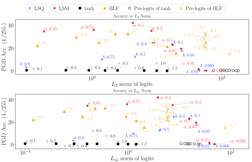
Figure 1: $L_{2}$ (top) and $L_{\infty}$ (bottom) norms of $\bm{z}$ or $\gamma g(\bm{z})$ vs robust accuracies. Pre-logits of BLF and tanh denote accuracies against norms of $\bm{z}$ instead of norms of $\gamma g(\bm{z})$. We omit $\gamma$ on Inputs of tanh to increase visibility.

3.2 Empirical evaluation of logit regularization

As shown above, logit regularization can induce the finite logit values, and tanh and sigmoid functions cannot keep pre-logits small. In this section, we empirically investigate the relation between logit norms and adversarial robustness. We evaluated the average norms of logits on clean data of CIFAR10 and accuracies on adversarial examples of CIFAR10 (PGD $\varepsilon\!=\!4/255$ and 100 iterations) for various logit regularization methods. Note that we normalized CIFAR10 such that their pixel values are in [0,1]. We used logit squeezing (LSQ), label smoothing (LSM), and bounded logits by tanh with various $\alpha$, $\lambda$, and $\gamma$. The detailed experimental conditions are provided in appendix B.

Figure 1 shows adversarial robustness against the average norms of logit vectors. Note that results of BLF in Fig. 1 are discussed in the next section. In this figure, each point corresponds to each hyper-parameter. For tanh, we also plot adversarial robustness against average norms of pre-logit vectors $\bm{z}$ as well as logit vectors $\gamma g(\bm{z})$. In Fig. 1, models learned using logit regularization methods have various norms and robustness depending on $\alpha$ and $\lambda$, and the robust accuracies become almost zero when norms exceed about seven. The results of tanh indicate that even if models have small logits by adding bounded functions, they are vulnerable when their pre-logit norms are large. In addition, the results of tanh imply that just scaling logits $\gamma\bm{z}$ does not improve the robustness. From the observation, we need a new function that has bounded outputs and inputs.

Figure 2: Comparison of BLF and tanh

4 Proposed method

We propose constraining logits by the addition of a new activation function called bounded logit function (BLF) just before softmax. BLF is defined as follows:

Definition 1.

Bounded logit function (BLF) is defined as

$$g(z)=2\left\{z\sigma(z)+\sigma(z)-z\sigma^{2}(z)\right\}-1,$$ (5)

where $\sigma$ is sigmoid function. When $z$ is a vector, BLF becomes element-wise operation.

BLF is similar to tanh as shown in Fig. 2. In fact, BLF has some of the same properties of tanh, e.g., $\lim_{z\rightarrow+\infty}g(z)=1$, $\lim_{z\rightarrow-\infty}g(z)\!=\!-1$, and $\left.\partial g(z)/\partial z\right|_{z=0}\!\!=\!z$. However, this function has the maximum and minimum points in $-\sqrt{5}\!-\!1\!<\!z\!<\!-2$ and $2\!<\!z\!<\!\sqrt{5}\!+\!1$ while tanh does not have the finite maximum and minimum points. Therefore, we have the following theorem:

Theorem 3.

Let $g(z)$ be BLF and $\gamma$ be a hyper-parameter satisfying $0\!<\!\gamma\!<\!\infty$. If we use $g(z)$ before softmax as $\bm{f}_{s}(\gamma g(\bm{z}_{\bm{\theta}}(\bm{x})))$, all elements of the optimal pre-logit vector $\bm{z}_{\bm{\theta}^{*}}(\bm{x}^{(i)})\!=\!\mathrm{arg}\!\min_{\bm{z}_{\bm{\theta}}}\mathcal{L}_{\mathrm{CE}}(\gamma g(\bm{z}_{\bm{\theta}}(\bm{x}^{(i)})),\bm{p}^{(i)})$ have finite values, and all elements of the optimal logit vector $\gamma g(\bm{z}_{\bm{\theta}^{*}})$ also have finite values. Specifically, we have the following equalities and inequalities:

$$\textstyle\gamma g(z_{\bm{\theta}^{*},k}(\bm{x}^{(i)})) \textstyle=\begin{cases}\gamma\max_{z}g(z)~{}~{}~{}k=t\\ \textstyle\gamma\min_{z}g(z)~{}~{}~{}\mathrm{otherwise},\end{cases}$$ (6)

$$\textstyle\gamma< \textstyle|\gamma g(z_{\bm{\theta}^{*},k}(\bm{x}^{(i)}))|<\gamma\frac{\sqrt{5}+1}{2},$$

$$z_{\theta^{*},k}(\bm{x}^{(i)}) \textstyle=\begin{cases}\textstyle\mathrm{arg}\!\max_{z}g(z)~{}~{}~{}k=t\\ \textstyle\mathrm{arg}\!\min_{z}g(z)~{}~{}~{}\mathrm{otherwise},\end{cases}$$ (7)

$$\textstyle 2< \textstyle|z_{\bm{\theta}^{*},k}(\bm{x}^{(i)})|<\sqrt{5}+1.$$

Theorem 3 indicates that this function gives finite logits and pre-logits unlike tanh. Therefore, we can keep both logits and pre-logits as small values when we add BLF before softmax. We can control the scale of logits by using the hyper-parameter $\gamma$. We conducted experiments using various $\gamma$ in the same manner as mentioned in the previous section, and evaluated adversarial robustness against norms of logits and pre-logits (Fig. 1). From this figure, BLF keeps the logits and pre-logits small, and its robust accuracy is higher than that of logit squeezing. Furthermore, since the optimal pre-logits $z_{\bm{\theta}^{*},j}(\bm{x}^{(i)})$ do not depend on $\gamma$, pre-logits of BLF on some $\gamma$ can have almost the same norms; the $L_{\infty}$ norms are vertically aligned on about 2.4 despite the difference in $\gamma$. The result indicates that the empirical optimal pre-logits follow Theorem 3, though our theoretical results are based on the Assumption in Section 3.1.

$\gamma$ can be used as a learnable parameter. However, the optimal $\gamma$ becomes infinitely large by minimization of softmax cross-entropy, and the logit norms become infinite values. Thus, the learnable $\gamma$ does not improve adversarial robustness. We also evaluated a learnable version of BLF (L-BLF) in the next section. In this setting, we used $\gamma=\mathrm{softplus}(\tilde{\gamma})$ and optimized $\tilde{\gamma}$ to keep $\gamma$ non-negative.

Note that one of the reasons why we use BLF is that BLF is similar to tanh, so it is easy to verify the effect of the finite optimal points. We can use other bounded functions, which are not monotonically increasing, instead of BLF. We evaluate some such functions in appendix D.

5 Experiments

In this section, we conducted experiments to evaluate the proposed method in terms of (a) robustness against gradient-based attacks, (b) robustness against gradient-free attacks, and (c) operator norms of models. In the experiments, we evaluated the models using only clean training data (standard training) and using adversarially perturbed training data (adversarial training), respectively.

5.1 Experimental Conditions

This section gives an outline of the experimental conditions and the details are provided in appendix B. Datasets of the experiments were MNIST (LeCun et al. 1998) and CIFAR10 (Krizhevsky and Hinton 2009). Our method was compared with a model trained without any logit regularization methods (Baseline), logit squeezing (LSQ), and label smoothing (LSM). In our method, we evaluated BLF with fixed $\gamma$ (BLF) and BLF with learnable $\gamma$ (L-BLF). We also compared them with TRADES, which is a strong defense method using adversarial examples (Zhang et al. 2019b), in the adversarial training setting.

For MNIST, we used a convolutional neural network (CNN) composed of two convolutional layers and two fully connected layers (2C2F) and one that is composed of four convolutional layers and three fully connected layers (4C3F) following (Zhang et al. 2019b). For CIFAR10, we used ResNet-18 (RN18) (He et al. 2016) and WideResNet-34-10 (WRN) (Zagoruyko and Komodakis 2016) also following (Zhang et al. 2019b).

We used untargeted projected gradient descent (PGD), which is the most popular white box attack, as a gradient-based attack and used SPSA and Square Attacks as gradient-free attacks. The hyper-parameters for PGD were based on (Madry et al. 2018). The $L_{\infty}$ norm of the perturbation $\varepsilon$ was set to $\varepsilon\!=\!0.3$ for MNIST and $\varepsilon\!=\!8/255$ for CIFAR10 at training time. For PGD, we randomly initialized the perturbation and updated it for 40 iterations with a step size of 0.01 on MNIST at training and evaluation times, and on CIFAR10 for 7 iterations with a step size of 2/255 at training time and 100 iterations with the same step size at evaluation time. At evaluation time, we use $\varepsilon\!=\![0,0.05,\dots,0.3]$ on MNIST and $\varepsilon\!=\![0,2/255,\dots,20/255]$ on CIFAR10. $\varepsilon\!=\!0$ corresponds to clean data. For TRADES, we set hyper-parameters of adversarial examples based on the code provided by the authors. On MNIST, step size was set to 0.01, and the number of steps was set to 40, and $\varepsilon$ was set to 0.3. On CIFAR10, step size was set to 2/255, and the number of steps was set to 10, and $\varepsilon$ was set to 8/255. We selected the best hyper-parameters of our method $\gamma$, logit squeezing $\lambda$, label smoothing $\alpha$, and TRADES $\beta$ among five parameters. The selected hyper-parameters are shown in Figs. 3 and 4 for MNIST and CIFAR10, respectively. For WRN, we used the same hyper-parameters as those of RN18. We trained models for five times for MNIST and three times for CIFAR10 and show the average and standard deviation of test accuracies. To generate adversarial examples, we used advertorch (Ding, Wang, and Jin 2019).

5.2 Robustness against gradient-based methods

Accuracy against PGD

Figures 3 (a)-(d) show accuracies on MNIST attacked by PGD. In these figures, results of $\varepsilon\!=\!0$ correspond to clean accuracy. For 2C2F (Fig. 3(a)) in the standard training setting, label smoothing is the most robust against PGD until $\varepsilon$ is smaller than 0.2. For 2C2F and 4C3F (Figs. 3(a) and (c)) with $\varepsilon>0.15$, BLF is the most robust in standard training. When we use the learnable $\tilde{\gamma}$, L-BLF does not improve the robustness. This is because $\tilde{\gamma}$ becomes large to minimize the loss function, and norms of logits have large values. In the adversarial training setting, our proposed function improves robustness the most for 2C2F and is comparable to TRADES for 4C3F. Note that TRADES of 2C2F (Fig. 3(b)) is not more robust than Baseline in our experiments. This might be because we train models on training data attacked by PGD with $\varepsilon=0.3$ following (Madry et al. 2018) while Zhang et al. (2019b) train them on training data attacked by PGD with $\varepsilon=0.1$ in Table 4 of (Zhang et al. 2019b).

Figure 4 shows the results on CIFAR10. In the standard training setting, label smoothing improves robustness the most for RN18, and our proposed method improves robustness the most for WRN. In the adversarial training setting, our method improves the robustness the most. It is more robust than TRADES even though the number of iteration for TRADES is larger than that of our method.

The reason label smoothing and logit squeezing are not so effective in the adversarial training might be due to the complexity of the objective function: regularization terms might disturb the mini-max problem for adversarial robustness. On the other hand, our method does not change the objective function. Thus, it is more suitable for adversarial training.

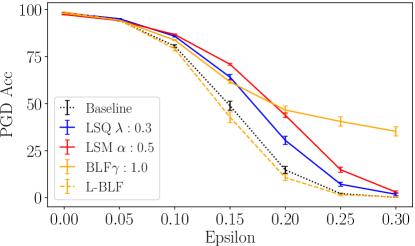
(a) Standard training

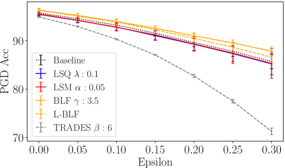
(b) Adversarial training

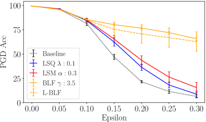
(c) Standard training

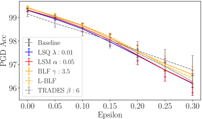
(d) Adversarial training

Figure 3: Accuracy of 2C2F (top) and 4C3F (bottom) on MNIST attacked by PGD (40 iterations). Error bars correspond to standard deviations.

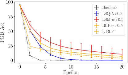
(a) Standard training

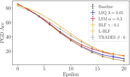
(b) Adversarial training

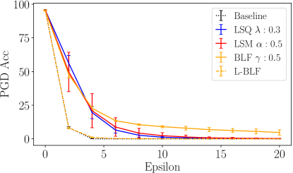
(c) Standard training

(d) Adversarial training

Figure 4: Accuracy of RN18 (top) and WRN (bottom) on CIFAR10 attacked by PGD (100 iterations). Error bars correspond to standard deviations.

Evaluation of misleading gradients of BLF

As shown in Fig. 2, the absolute values of BLF $|g(z)|$ does not become smaller than one in intervals of $z\!<\!\mathrm{arg}\!\min_{z}g(z)$ and $z\!>\!\mathrm{arg}\!\max_{z}g(z)$. In the intervals, the gradient of BLF might mislead the gradient-based attacks because the absolute values of outputs of BLF only change in $1\!<\!|g(z)|\!<\!\max_{z}|g(z)|$. This might be a cause of robustness of BLF, which is not expected. To investigate the effect of the intervals, we replaced a BLF with tanh to generate PGD attacks. We conducted this experiment by the following procedure: (i) we trained BLF models in standard and adversarial settings, (ii) we replaced BLF with tanh in models trained at the previous step, (iii) we generated PGD attacks by using replaced models, (iv) we replaced tanh with BLF again and evaluated robust accuracies of BLF models against PGD attacks generated at the previous step. Since tanh is similar to BLF and is a monotonically increasing function, gradient-based attacks can effectively avoid the misleading gradients in the above mentioned intervals. In fact, we observed that replaced models achieved almost the same clean accuracy as BLF models even though their parameters are optimized for BLF: Clean accuracies of BLF (standard training), replaced models (standard training)), BLF (adversarial training), and replaced models (adversarial training) are 94.58, 94.58, 82.42, and 83.38, respectively.

Robust accuracies of RN18 on CIFAR10 is shown in Fig. 5. In this figure, we show robust accuracies of BLF models against PGD by using replaced models and using the BLF models. Though PGD for replaced models succeeded in attacking BLF models more than PGD for BLF models when $\varepsilon$ is set to be greater than $10$ in standard training settings, it could not attack BLF models well in the adversarial training setting and in the standard training setting when $\varepsilon<10$. Therefore, BLF does not only employ the misleading gradients in $z\!<\!\mathrm{arg}\!\min_{z}g(z)$ and $z\!>\!\mathrm{arg}\!\max_{z}g(z)$ for improving adversarial robustness.

(a) Standard training

(b) Adversarial training

Figure 5: Robust accuracy against PGD by using models replaced tanh. We compare robust accuracies against PGD naively generated by using BLF models and against PGD generated by using tanh.

5.3 Robustness against gradient-free attacks

Since Mosbach et al. (2018) pointed out that logit regularization only masks or obfuscates gradient to improve robustness, we evaluated the robustness against gradient-free attacks. In the experiments, we tuned hyperparameters ($\lambda$, $\alpha$, $\gamma$, $\beta$) for each attack and train the model for one time for each hyper-parameter.

Accuracy against SPSA attacks

We used SPSA as a gradient-free attack because it can operate when the loss surface is difficult to optimize (Carlini et al. 2019; Uesato et al. 2018). We set the hyper-parameters of SPSA as epsilons of 0.15 for MNIST and 8/255 for CIFAR10, perturbation size of 0.01, Adam learning rate of 0.01, maximum iterations of 40 for MNIST and 10 for CIFAR10, and batchsize of 2048.

Table 1 lists the accuracies of 2C2F and 4C3F with each method on MNIST attacked by SPSA and RN18 and WRN with each method on CIFAR10 attacked by SPSA. We can see that in the standard training setting, BLF improves robustness against SPSA the most on MNIST even though robustness against PGD of BLF is lower than those of label smoothing and logit squeezing in Fig. 3 (a). On CIFAR10, label smoothing and logit squeezing improve robustness more than BLF. In adversarial training settings, however, our method improves robustness the most in a majority of settings. These results are in agreement with the results of gradient-based attacks.

Table 1: Robust accuracies against SPSA on MNIST ($\varepsilon\!=\!0.15$) and CIFAR10 ($\varepsilon\!=\!8/255$). ST and AT represent standard training and adversarial training, respectively.

	Baseline	LSQ	LSM	BLF	TRADES
2C2F ST	$53.5$	$60.8$	$67.4$	$\bm{68.4}$	N/A
2C2F AT	$90.2$	$92.3$	$90.0$	$\bm{92.7}$	$86.4$
4C3F ST	$51.3$	$69.2$	$73.8$	$\bm{82.4}$	N/A
4C3F AT	$\bm{98.3}$	$\bm{98.3}$	$98.2$	$98.2$	$98.1$
RN18 ST	$0.3$	$23.5$	$\bm{24.9}$	$23.4$	N/A
RN18 AT	$56.6$	$56.8$	$56.6$	$\bm{58.7}$	$57.4$
WRN ST	$0.1$	$\bm{42.1}$	$16.3$	$13.9$	N/A
WRN AT	$60.6$	$61.5$	$60.0$	$\bm{62.3}$	$61.3$

Table 2: Robust accuracies against Square Attack on MNIST ($\varepsilon\!=\!0.15$) and CIFAR10 ($\varepsilon\!=\!8/255$). ST and AT represent standard training and adversarial training, respectively.

	Baseline	LSQ	LSM	BLF	TRADES
2C2F ST	51.5	53.0	$\bm{64.0}$	59.4	N/A
2C2F AT	91.4	90.3	91.0	$\bm{92.1}$	85.3
4C3F ST	35.6	46.2	51.5	$\bm{56.1}$	N/A
4C3F AT	97.9	$\bm{98.0}$	97.9	$\bm{98.0}$	$\bm{98.0}$
RN18 ST	$0.3$	$20.1$	$27.6$	$\bm{31.7}$	N/A
RN18 AT	$54.5$	$55.4$	$\bm{55.6}$	$53.8$	$55.3$
WRN ST	$0.2$	30.2	$\bm{38.4}$	30.8	N/A
WRN AT	$59.7$	$59.7$	$60.0$	$\bm{60.9}$	$59.4$

Accuracy against Square Attacks

Although the SPSA attack does not use exact gradients, it still approximates gradients to generate attacks. Thus, obfuscating gradients might be still effective for the SPSA attack. To investigate whether logit regularization methods just obfuscate gradients, we evaluate the robustness against Square Attack (Andriushchenko et al. 2020), which is a query-based black box attack. Since the Square Attack uses random search to generate attacks, obfuscating gradients are ineffective for the Square Attack. To generate Square Attacks, we set the number of queries to 5000 and use the code in (Croce and Hein 2020). Note that untargeted Square Attacks use a margin loss instead of cross entropy loss.

Robust accuracies against Square Attacks are listed in Tab. 2. In this table, BLF achieves the highest or the second highest accuracies on almost all settings. In addition, all logit regularization methods without adversarial training can improve the robust accuracies though Square Attacks do not use gradients. Therefore, logit constraints does not only just obfuscate gradients for improving robustness.

5.4 Evaluation of operator norms

As discussed in Section 3, softmax cross-entropy can cause large Lipschitz constants, and it might be a cause of vulnerabilities. To investigate Lipschitz constants of models, we computed averages of $L_{\infty}$ operator norms of convolution layers of RN18 (Tab. 3) by following (Gouk et al. 2018). The $L_{\infty}$ operator norms of convolution layers can be a criterion of Lipschitz constants since one of Lipschitz constants of composite functions is the product of Lipschitz constants of composing functions and $L_{\infty}$ operator norm is a Lipschitz constant for a linear function. Table 3 shows that logit regularization methods induce small $L_{\infty}$ operator norms of convolution layers compared with Baseline even though they do not explicitly impose the penalty of parameter values. This table indicates that BLF can outperform other methods when using adversarial training because it effectively induces small Lipschitz constants. On the other hand, the $L_{\infty}$ norm of L-BLF is almost the same as that of Baseline. Thus, BLF with learnable $\gamma$ does not improve the robustness. Note that the $L_{\infty}$ norm of Baseline does not become extremely large because we applied some regularization methods, e.g., weight decay and early stopping, into all methods to obtain good generalization performance.

Table 3: Averages of $L_{\infty}$ operator norms of convolution layers of RN18.

	Baseline	LSQ	LSM	BLF	L-BLF	TRADES
ST	$19.6$	$17.1$	$10.1$	$11.2$	$20.1$	N/A
AT	$17.1$	$16.5$	$11.4$	$4.4$	$16.8$	$13.3$

6 Conclusion

We proposed a method of constraining the logits by adding a bounded activation function just before softmax following the hypothesis that small logits improve the adversarial robustness. We developed a new bounded function that has the finite maximum and minimum points so that logits and pre-logits have small values. Compared with other logit regularization methods, our method can effectively improve the robustness in adversarial training despite its simplicity.

Though we provided insights into the vulnerabilities of softmax cross-entropy and empirical evidence of the effectiveness of logit regularization methods, it is still an open question why small logits can improve robustness. Our experiments of tanh indicate that small logits are not sufficient for adversarial robustness. Even so, our experiments showed that our method is comparable to the recent defense method in terms of adversarial robustness against both gradient-based and gradient-free attacks in adversarial training. Thus, our results indicate that the investigation into the relation between logit regularization and robustness is still an important research direction to reveal the cause of vulnerabilities of DNNs.

Appendix A Proofs

In this section, we show proofs of theoretical results in the paper following the assumption.

Assumption.

We assume that (a) if data points have the same values as $\bm{x}^{(i)}\!=\!\bm{x}^{(j)}$, they have the same labels as $\bm{p}^{(i)}\!=\!\bm{p}^{(j)}$, (b) the logit vector $\bm{z}_{\bm{\theta}}(\bm{x})$ can be an arbitrary vector for each data point, and (c) the optimal point $\bm{\theta}^{*}\!=\!\mathrm{arg}\!\min_{\bm{\theta}}\!\frac{1}{N}\!\sum_{i=1}^{N}\!\mathcal{L}(\bm{z}_{\bm{\theta}}(\bm{x}^{(i)}),\bm{p}^{(i)})$ achieves $\mathcal{L}(\bm{z}_{\bm{\theta}^{*}}(\bm{x}^{(i)}),\bm{p}^{(i)})\!=\min_{\bm{\theta}}\mathcal{L}(\bm{z}_{\bm{\theta}}(\bm{x}^{(i)}),\bm{p}^{(i)})$ for all $i$.

Theorem 1.

If we use softmax cross-entropy and one-hot vectors as target values, at least one element of the optimal logits $\bm{z}_{\bm{\theta}^{*}}(\bm{x}^{(i)})\!=\!\mathrm{arg}\min_{\bm{z}_{\bm{\theta}}}\mathcal{L}_{\mathrm{CE}}(\bm{z}_{\bm{\theta}}(\bm{x}^{(i)}),\bm{p}^{(i)})$ does not have a finite value.

Proof.

Let $t$ be a target label for $\bm{x}^{(i)}$. The objective function of softmax cross-entropy loss for $\bm{x}^{(i)}$ is

$$\textstyle J=\mathcal{L}_{\mathrm{CE}}(\bm{z}_{\bm{\theta}}(\bm{x}^{(i)}),\bm{p}^{(i)})=-\mathrm{log}[\bm{f}_{s}(\bm{z}_{\bm{\theta}}(\bm{x}^{(i)}))]_{t}.$$

At the minimum point, we have $\left.\frac{\partial J}{\partial\bm{z}_{\bm{\theta}}(\bm{x}^{(i)})}\right|_{\bm{z}_{\bm{\theta}^{*}}}=\bm{0}$ since we assume $\bm{z}_{\bm{\theta}}(\bm{x}^{(i)})$ can be an arbitrary vector in Assumption. By differentiating softmax cross-entropy, we obtain

$$\textstyle\frac{\partial J}{\partial z_{\bm{\theta},k}(\bm{x}^{(i)})}=\begin{cases}-1+[\bm{f}_{s}(\bm{z}_{\bm{\theta}}(\bm{x}^{(i)}))]_{k}&k\textstyle=t,\\ \textstyle[\bm{f}_{s}(\bm{z}_{\bm{\theta}}(\bm{x}^{(i)}))]_{k}&\mathrm{otherwise}.\end{cases}$$ (8)

Thus, $\left.\frac{\partial J}{\partial\bm{z}_{\bm{\theta}}(\bm{x}^{(i)})}\right|_{\bm{z}_{\bm{\theta}^{*}}}\!\!=\!\bm{0}$ means that a softmax output vector $\bm{f}_{s}(\bm{z}_{\bm{\theta}^{*}}(\bm{x}^{(i)}))$ is a one hot-vector; $[\bm{f}_{s}(\bm{z}_{\bm{\theta}^{*}}(\bm{x}^{(i)}))]_{t}\!=\!1$ and $[\bm{f}_{s}(\bm{z}_{\bm{\theta}^{*}}(\bm{x}^{(i)}))]_{k}\!=\!0$ for $k\!\neq\!t$. Since $[\bm{f}_{s}(\bm{z}_{\bm{\theta}}(\bm{x}^{(i)}))]_{t}\neq 0$, we have $0<\sum_{m=1}^{M}\mathrm{exp}(z_{\bm{\theta},m}(\bm{x}^{(i)}))$. The $t$-th output of softmax becomes

$$\textstyle\frac{\mathrm{exp}(z_{\bm{\theta},t}(\bm{x}^{(i)}))}{\sum_{m=1}^{M}\mathrm{exp}(z_{\bm{\theta},m}(\bm{x}^{(i)}))} \textstyle=1,$$

$$\textstyle\mathrm{exp}(z_{\bm{\theta},t}(\bm{x}^{(i)})) \textstyle=\sum_{m=1}^{M}\mathrm{exp}(z_{\bm{\theta},m}(\bm{x}^{(i)})),$$

$$\textstyle\sum_{m\neq t}\mathrm{exp}(z_{\bm{\theta},m}(\bm{x}^{(i)})) \textstyle=0.$$

Since $\mathrm{exp}(z)\geq 0$, we have $\mathrm{exp}(z_{\bm{\theta},m}(\bm{x}^{(i)}))=0$ for $m\neq t$. Since $\lim_{z\rightarrow-\infty}\mathrm{exp}(z)=0$, the element of the optimal logits $z_{\bm{\theta}^{*},m}(\bm{x}^{(i)})$ does not have a finite value for $m\neq t$. Therefore, at least one element of the optimal logits has an infinite value. ∎

Corollary 1.

If all elements of inputs $x_{k}^{(i)}$ are normalized as $0\leq x_{k}^{(i)}\leq 1$ and training dataset has at least two different labels, the optimal logit function $\bm{z}_{\bm{\theta}^{*}}(\bm{x})$ for softmax cross-entropy is not globally Lipschitz continuous function, i.e., there is not a finite constant $C\geq 0$ as

$$\textstyle||\bm{z}_{\bm{\theta}^{*}}(\bm{x}^{(i)})-\bm{z}_{\bm{\theta}^{*}}(\bm{x}^{(j)})||_{\infty} \leq C||\bm{x}^{(i)}-\bm{x}^{(j)}||_{\infty},$$

$$\forall\bm{x}^{(i)},\bm{x}^{(j)} \in\mathcal{X}.$$

Proof.

If Corollary 1 does not hold, there is a finite constant $C$ satisfying

$$\textstyle||\bm{z}_{\bm{\theta}^{*}}(\bm{x}^{(i)})-\bm{z}_{\bm{\theta}^{*}}(\bm{x}^{(j)})||_{\infty} \leq C||\bm{x}^{(i)}-\bm{x}^{(j)}||_{\infty}$$ (9)

$$\forall\bm{x}^{(i)},\bm{x}^{(j)} \in\mathcal{X},$$

and $0\leq C<\infty$. We assume that $t$ and $t^{\prime}$ are labels of $\bm{x}^{(i)}$ and $\bm{x}^{(j)}$, respectively, and $t\neq t^{\prime}$. As shown in the proof of Theorem 1, $z_{\bm{\theta},m}(\bm{x}^{(i)})$ for $m\neq t$ does not have finite values and $-\infty<z_{\bm{\theta},t}(\bm{x}^{(i)})\leq\infty$. On the other hand $z_{\bm{\theta},m}(\bm{x}^{(j)})$ for $m\neq t^{\prime}$ does not have finite values. Thus, $[\bm{z}_{\bm{\theta}^{*}}(\bm{x}^{(i)})-\bm{z}_{\bm{\theta}^{*}}(\bm{x}^{(j)})]_{t}=z_{\bm{\theta},t}(\bm{x}^{(i)})-z_{\bm{\theta},t}(\bm{x}^{(j)})$ does not have finite values. Thus, the left-hand side of eq. (9) is not finite values. On the other hand, we have $||\bm{x}^{(i)}-\bm{x}^{(j)}||_{\infty}\leq 1$ because we assume $0\leq x_{k}\leq 1$. As a result, $\infty\leq C||\bm{x}^{(i)}-\bm{x}^{(j)}||_{\infty}\leq C$, and it contradicts the statement $0\leq C<\infty$, which completes the proof. ∎

Proposition 1.

The optimal logits for label smoothing $\bm{z}_{\bm{\theta}^{*}}(\bm{x}^{(i)})\!=\!\mathrm{arg}\min_{\bm{z}_{\bm{\theta}}}\mathcal{L}_{\mathrm{CE}}(\bm{z}_{\bm{\theta}}(\bm{x}^{(i)}),\bm{p}^{(i)})$ satisfy

$$\textstyle z_{\bm{\theta}^{*},k}(\bm{x}^{(i)})\!=\!\begin{cases}\!\log(\frac{1\!-\!\alpha}{\alpha}\!\sum_{m\neq t}\!\mathrm{exp}((z_{\bm{\theta}^{*},m}(\bm{x}^{(i)}))))&\!\!\!\!\!k=t\\ \!\log(\frac{\alpha}{M\!-\!1\!-\!\alpha}\!\sum_{m\neq k}\mathrm{exp}(z_{\bm{\theta}^{*},m}(\bm{x}^{(i)})))&\!\!\!\!\!k\neq t.\end{cases}$$

If an element of $\mathrm{exp}(\bm{z_{\bm{\theta}^{*}}}(\bm{x}^{(i)}))$ has a finite value, all elements of $\bm{z}_{\bm{\theta}^{*}}(\bm{x}^{(i)})$ have finite values.

Proof.

Let $t$ be a label of data point $\bm{x}^{(i)}$. The objective function of label smoothing for $\bm{x}^{(i)}$ is

$$\textstyle J \textstyle=-\sum_{m}p_{m}\mathrm{log}[\bm{f}_{s}(\bm{z}_{\bm{\theta}}(\bm{x}^{(i)}))]_{m}$$

$$\textstyle=-(1-\alpha)\mathrm{log}[\bm{f}_{s}(\bm{z}_{\bm{\theta}}(\bm{x}^{(i)}))]_{t}$$

$$\textstyle~{}~{}~{}~{}~{}-\frac{\alpha}{M-1}\sum_{m\neq t}\mathrm{log}[\bm{f}_{s}(\bm{z}_{\bm{\theta}}(\bm{x}^{(i)}))]_{m}$$

since $p_{t}=1-\alpha$ and $p_{m}=\frac{\alpha}{M-1}$ for $m\neq t$. By differentiating softmax cross-entropy, we obtain

$$\textstyle\frac{\partial J}{\partial z_{\bm{\theta},k}}=\begin{cases}[\bm{f}_{s}(\bm{z}_{\bm{\theta}^{*}}(\bm{x}^{(i)}))]_{k}+\alpha-1&k=t,\\ \textstyle[\bm{f}_{s}(\bm{z}_{\bm{\theta}^{*}}(\bm{x}^{(i)}))]_{k}-\frac{\alpha}{M-1}&\textstyle\mathrm{otherwise}.\end{cases}$$ (10)

Since we assume that one of the elements of $\bm{z}_{\bm{\theta}^{*}}$ has a finite value, we have $\sum_{m}\mathrm{exp}z_{\bm{\theta}^{*},m}>0$. Thus, eq. (10) for $k=t$ becomes

$$\textstyle[\bm{f}_{s}(\bm{z}_{\bm{\theta}^{*}}(\bm{x}^{(i)}))]_{t} \textstyle=1-\alpha,$$ (11)

$$\textstyle\frac{\mathrm{exp}z_{\bm{\theta}^{*},t}}{\sum_{m}\mathrm{exp}z_{\bm{\theta}^{*},m}} \textstyle=1-\alpha,$$

$$\textstyle\mathrm{exp}z_{\bm{\theta}^{*},t} \textstyle=(1-\alpha)(\sum_{m}\mathrm{exp}z_{\bm{\theta}^{*},m}),$$

$$\textstyle\alpha\mathrm{exp}z_{\bm{\theta}^{*},t} \textstyle=(1-\alpha)(\sum_{m\neq t}\mathrm{exp}z_{\bm{\theta}^{*},m}),$$

$$\textstyle z_{\bm{\theta}^{*},t} \textstyle=\log(\frac{1-\alpha}{\alpha}(\sum_{m\neq t}\mathrm{exp}z_{\bm{\theta}^{*},m})).$$ (12)

In the same manner, we have

$$[\bm{f}_{s}(\bm{z}_{\bm{\theta}^{*}}(\bm{x}^{(i)}))]_{k}\textstyle=\frac{\alpha}{M-1},$$ (13)

$$z_{\bm{\theta}^{*},k}\textstyle=\log(\frac{\alpha}{M-1-\alpha}\sum_{m\neq k}\mathrm{exp}(z_{\bm{\theta}^{*},m}(\bm{x}^{(i)}))),$$ (14)

for $k\neq t$. It is difficult to obtain the solutions of eqs. (12) and (14) in closed form, but we can show they have finite values as follows. If $z_{\bm{\theta}^{*},k^{\prime}}(\bm{x}^{(i)}))\rightarrow-\infty$ where $k^{\prime}\neq t$, eq. (13) does not hold because the left side of eq. (13) becomes 0 and $0<\alpha<M-1$. If $z_{\bm{\theta}^{*},t}(\bm{x}^{(i)}))\rightarrow\infty$, eq. (11) does not hold because the left side of eq. (11) becomes 1. Therefore, all elements of the logits have finite values. ∎

Proposition 2.

The optimal logits for logit squeezing $\!\bm{z}_{\bm{\theta}^{*}}(\bm{x}^{(i)})\!=\!\mathrm{arg}\!\min_{\bm{z}_{\bm{\theta}}}\mathcal{L}_{\mathrm{CE}}(\bm{z}_{\bm{\theta}}(\bm{x}^{(i)}),\bm{p}^{(i)}\!)\!+\!\frac{\lambda}{2}\!||\bm{z}_{\bm{\theta}}(\bm{x}^{(i)})||_{2}$ satisfy

$$\!z_{\bm{\theta}^{*}\!,k}(\bm{x}^{(i)})\!=\!\begin{cases}(-[f_{s}(\bm{z}_{\bm{\theta}^{*}}(\bm{x}^{(i)})\!)]_{t}+1)/\lambda&k=t\\ \!=\!-[f_{s}(\bm{z}_{\bm{\theta}^{*}}(\bm{x}^{(i)})\!)]_{k}/\lambda&k\neq t.\end{cases}$$

Namely, all elements of the optimal logit vector $\bm{z}_{\bm{\theta}^{*}}(\bm{x}^{(i)})$ have finite values.

Proof.

Let $t$ be a label of data point $\bm{x}^{(i)}$. The objective function of logit squeezing for $\bm{x}^{(i)}$ is $J=-\mathrm{log}[\bm{f}_{s}(\bm{z}_{\bm{\theta}}(\bm{x}^{(i)}))]_{t}+\frac{\lambda}{2}||\bm{z}_{\bm{\theta}}(\bm{x}^{(i)})||_{2}$. Since we assume $\bm{z}_{\bm{\theta}}(\bm{x}^{(i)})$ can be an arbitrary vector, $\left.\frac{\partial J}{\partial\bm{z}_{\bm{\theta}}}\right|_{\bm{z}_{\bm{\theta}}=\bm{z}_{\bm{\theta}^{*}}}=\bm{0}$ at the minimum points. By differentiating $J$, we obtain

$$\textstyle\frac{\partial J}{\partial z_{\bm{\theta},k}}=\begin{cases}-1+[\bm{f}_{s}(\bm{z}_{\bm{\theta}}(\bm{x}^{(i)}))]_{k}+\lambda z_{\bm{\theta},k}&k=t,\\ [\bm{f}_{s}(\bm{z}_{\bm{\theta}}(\bm{x}^{(i)}))]_{k}+\lambda z_{\bm{\theta},k}&\mathrm{otherwise},\end{cases}$$

thus have

$$\textstyle-1+[\bm{f}_{s}(\bm{z}_{\bm{\theta}^{*}}(\bm{x}^{(i)}))]_{t}+\lambda z_{\bm{\theta}^{*},t} =0,$$

$$\textstyle z_{\bm{\theta}^{*},t} =\frac{1-[\bm{f}_{s}(\bm{z}_{\bm{\theta}^{*}}(\bm{x}^{(i)}))]_{t}}{\lambda}.$$

Since each element of softmax functions is bounded as $0\leq[\bm{f}_{s}(\bm{z}_{\bm{\theta}^{*}}(\bm{x}^{(i)}))]_{k}\leq 1$, we have $0\leq z_{\bm{\theta}^{*},t}\leq\frac{1}{\lambda}$. In the same manner, we have $-\frac{1}{\lambda}\leq z_{\bm{\theta}^{*},k}\leq 0$ for $k\neq t$. Therefore, all elements of the optimal logits have finite values. ∎

Theorem 2.

Let $g(z)$ be tanh or sigmoid function and $\gamma$ be a hyper-parameter satisfying $0\!<\!\gamma\!<\!\infty$. If we use tanh or sigmoid function before softmax as $\bm{f}_{s}(\gamma g(\bm{z}_{\bm{\theta}}(\bm{x}^{(i)})))$, all elements of the optimal pre-logit vector $\bm{z}_{\bm{\theta}^{*}}(\bm{x}^{(i)})\!=\!\mathrm{arg}\min_{\bm{z}_{\bm{\theta}}}\mathcal{L}_{\mathrm{CE}}(\gamma g(\bm{z}_{\bm{\theta}}(\bm{x}^{(i)})),\bm{p}^{(i)})$ do not have finite values while all elements of the optimal logit vector $\gamma g(\bm{z}_{\bm{\theta}^{*}})$ has finite values.

Proof.

First, we show the case using tanh as $g(z)=\mathrm{tanh}(z)$. Let $t$ be a target label for $\bm{x}^{(i)}$. The objective function of softmax cross-entropy loss for $\bm{x}^{(i)}$ is

Since we assume that $\bm{z}_{\bm{\theta}}(\bm{x}^{(i)})$ can be an arbitrary vector, $\left.\frac{\partial J}{\partial\bm{z}_{\bm{\theta}}}\right|_{\bm{z}_{\bm{\theta}}^{*}(\bm{x}^{(i)})}=\bm{0}$ at the minimum point. Since $\mathrm{tanh}$ is an element-wise function, $\frac{\partial J}{\partial z_{\bm{\theta}^{*},k}}$ is written as

$$\textstyle\frac{\partial J}{\partial z_{\bm{\theta},k}}=\gamma\frac{\partial J}{\partial\gamma\mathrm{tanh}(z_{\bm{\theta},k})}\frac{\partial\mathrm{tanh}(z_{\bm{\theta},k})}{\partial z_{\bm{\theta},k}}.$$

$\gamma\frac{\partial J}{\partial\gamma\mathrm{tanh}(z_{\bm{\theta},k})}$ is obtained as in eq. (8) and does not become 0 since $-1\leq\mathrm{tanh}(z_{\bm{\theta},k})\leq 1$ and $0<\gamma<\infty$. Thus, $\left.\frac{\partial J}{\partial z_{\bm{\theta},k}}\right|_{z_{\bm{\theta}^{*},k}(\bm{x}^{(i)})}=0$ corresponds to $\left.\frac{\partial\mathrm{tanh}(z_{\bm{\theta},k})}{\partial z_{\bm{\theta},k}}\right|_{z_{\bm{\theta}^{*},k}(\bm{x}^{(i)})}=0$. We have

$$\textstyle\frac{\partial\mathrm{tanh}(z_{\bm{\theta},k})}{\partial z_{\bm{\theta},k}}=1-\mathrm{tanh}^{2}(z_{\bm{\theta},k}).$$

Only if $z_{\bm{\theta}^{*},k}(\bm{x}^{(i)})\rightarrow\pm\infty$, the following equation holds: $\left.\frac{\partial\mathrm{tanh}(z_{\bm{\theta},k})}{\partial z_{\bm{\theta},k}}\right|_{z_{\bm{\theta}^{*},k}(\bm{x}^{(i)})}=0$. Therefore, all elements of the optimal input vector $\bm{z}_{\bm{\theta}^{*}}$ do not have finite values. The case using sigmoid function $\sigma(z)$ can be shown in the same manner. Since the derivative of sigmoid becomes $\frac{\partial\sigma(z_{\bm{\theta},k})}{\partial z_{\bm{\theta},k}}=\sigma(z_{\bm{\theta},k})(1-\sigma(z_{\bm{\theta},k}))$, the equation $\left.\frac{\partial\sigma(z_{\bm{\theta},k})}{\partial z_{\bm{\theta},k}}\right|_{z_{\bm{\theta}^{*},k}(\bm{x}^{(i)})}=0$ holds when $z_{\bm{\theta}^{*},k}(\bm{x}^{(i)})\rightarrow\pm\infty$. ∎

Theorem 3.

Let $g(z)$ be BLF and $\gamma$ be a hyper-parameter satisfying $0\!<\!\gamma\!<\!\infty$. If we use $g(z)$ before softmax as $\bm{f}_{s}(\gamma g(\bm{z}_{\bm{\theta}}(\bm{x})))$, all elements of the optimal pre-logit vector $\bm{z}_{\bm{\theta}^{*}}(\bm{x}^{(i)})\!=\!\mathrm{arg}\!\min_{\bm{z}_{\bm{\theta}}}\mathcal{L}_{\mathrm{CE}}(\gamma g(\bm{z}_{\bm{\theta}}(\bm{x}^{(i)})),\bm{p}^{(i)})$ have finite values, and all elements of the optimal logit vector $\gamma g(\bm{z}_{\bm{\theta}^{*}})$ also have finite values. Specifically, we have the following equalities and inequalities:

$$\textstyle\gamma g(z_{\bm{\theta}^{*},k}(\bm{x}^{(i)})) \textstyle=\begin{cases}\gamma\max_{z}g(z)~{}~{}~{}k=t\\ \textstyle\gamma\min_{z}g(z)~{}~{}~{}\mathrm{otherwise},\end{cases}$$ (15)

$$\gamma< |\gamma g(z_{\bm{\theta}^{*},k}(\bm{x}^{(i)}))|<\gamma\frac{\sqrt{5}+1}{2},$$

$$z_{\theta^{*},k}(\bm{x}^{(i)}) \textstyle=\begin{cases}\mathrm{arg}\!\max_{z}g(z)~{}~{}~{}k=t\\ \textstyle\mathrm{arg}\!\min_{z}g(z)~{}~{}~{}\mathrm{otherwise},\end{cases}$$ (16)

$$2< |z_{\bm{\theta}^{*},k}(\bm{x}^{(i)})|<\sqrt{5}+1.$$

Proof.

Let $t$ be a target label for $\bm{x}^{(i)}$. The objective function of softmax cross-entropy loss for $\bm{x}^{(i)}$ is

$$J=\mathcal{L}_{\mathrm{CE}}(\gamma g(\bm{z}_{\bm{\theta}}(\bm{x}^{(i)})),\bm{p}^{(i)})=-\mathrm{log}[\bm{f}_{s}(\gamma g(\bm{z}_{\bm{\theta}}(\bm{x}^{(i)})))]_{t},$$

where $g(z)=2\left\{z\sigma(z)+\sigma(z)-z\sigma^{2}(z)\right\}-1$. Since we assume that $\bm{z}_{\bm{\theta}}(\bm{x}^{(i)})$ can be an arbitrary vector, $\left.\frac{\partial J}{\partial\bm{z}_{\bm{\theta}}}\right|_{\bm{z}_{\bm{\theta}^{*}}(\bm{x}^{(i)})}=\bm{0}$ at the minimum point. Similary to tanh, BLF $g(z)$ is an element-wise function and bounded by finite values. Therefore, $\gamma\frac{\partial J}{\partial\gamma g(z_{\bm{\theta},k})}$ does not become 0. As a result, $\left.\frac{\partial J}{\partial\bm{z}_{\bm{\theta}}}\right|_{\bm{z}_{\bm{\theta}}^{*}(\bm{x}^{(i)})}=\bm{0}$ holds when $\left.\frac{\partial g(z_{\bm{\theta},k})}{\partial z_{\bm{\theta},k}}\right|_{z_{\bm{\theta},k}^{*}(\bm{x}^{(i)})}=0$ for all $k$. We have

thus, candidates of the optimal points satisfy one of the following conditions: $\sigma(z)=0$, $\sigma(z)=1$, and $2+z-2z\sigma(z)=0$. Inputs that satisfy $\sigma(z)=0$ and $\sigma(z)=1$ correspond to $z\rightarrow-\infty$ and $z\rightarrow\infty$, respectively. Their outputs $g(z)$ become $\lim_{z\rightarrow-\infty}g(z)=-1$ and $\lim_{z\rightarrow\infty}g(z)=1$, respectively. To investigate points satisfying $2+z-2z\sigma(z)=0$, we define $f(z)=2+z-2z\sigma(z)$, which is a continuous function. This function can be written as

$$\textstyle f(z) \textstyle=2+z-2z\sigma(z),$$

$$\textstyle=2+z-2z\frac{1}{1+e^{-z}},$$

$$\textstyle=2+\frac{z(1+e^{-z})-2z}{1+e^{-z}},$$

$$\textstyle=2-z\frac{1-e^{-z}}{1+e^{-z}},$$ (17)

$$\textstyle=2-z\mathrm{tanh}(\frac{z}{2}).$$

Since $\mathrm{tanh(z)}<z$ for $z>0$ and $\mathrm{tanh(z)}>z$ for $z<0$, we have

$$\textstyle f(z)=2-z\mathrm{tanh}(z/2)>2-\frac{z^{2}}{2}~{}~{}\mathrm{for}~{}~{}z\neq 0.$$

By using this equation, we have $f(z)>0$ for $-2<z<2$. In addition, since $\frac{z}{1+z}<1-e^{-z}$ for $z>-1$, we have the following inequality from eq. (17):

$$\textstyle f(z) \textstyle=2-z\frac{1-e^{-z}}{1+e^{-z}},$$

$$\textstyle=\frac{2(1+e^{-z})-z(1-e^{-z})}{1+e^{-z}},$$ (18)

$$\textstyle=\frac{-(2+z)(1-e^{-z})+4}{1+e^{-z}},$$

$$\textstyle<\frac{-(2+z)z+4(z+1)}{(1+e^{-z})(z+1)},$$

$$\textstyle=\frac{-(z-1)^{2}+5}{(1+e^{-z})(z+1)}.$$

Thus, we have $f(z)<0$ for $z>\sqrt{5}+1$. On the other hand, since we have $e^{z}<\frac{1}{1-z}$ for $z<1$, we have the following inequality from eq. (18):

$$\textstyle f(z) \textstyle=\frac{2(1+e^{-z})-z(1-e^{-z})}{1+e^{-z}},$$

$$\textstyle=\frac{2(e^{z}+1)-z(e^{z}-1)}{e^{z}+1},$$

$$\textstyle=\frac{e^{z}(2-z)+2+z}{e^{z}+1},$$

$$\textstyle<\frac{2-z+(2+z)(1-z)}{(e^{z}+1)(1-z)},$$

$$\textstyle=\frac{-(z+1)^{2}+5}{(1+e^{-z})(1-z)}.$$

Thus, we have $f(z)<0$ for $z<-\sqrt{5}-1$. Therefore, the points satisfying $\frac{\partial g(z)}{\partial z}=0$ are included in $-\sqrt{5}-1<z<-2$ and $2<z<\sqrt{5}+1$ from intermediate value theorem. The $g(z)$ can be written using $f(z)$ as

$$g(z) =2\left\{z\sigma(z)+\sigma(z)-z\sigma^{2}(z)\right\}-1,$$

$$=2\sigma(z)\left\{\frac{z}{2}+\frac{f(z)}{2}\right\}-1.$$

Let $\underline{z}^{*}$ be inputs satisfying $f(\underline{z}^{*})=0$ and $\sqrt{5}-1<\underline{z}^{*}<-2$, and $\bar{z}^{*}$ be inputs satisfying $f(\bar{z}^{*})=0$ and $2<\bar{z}^{*}<\sqrt{5}+1$. We have

$$\textstyle g(\underline{z}^{*}) \textstyle=\sigma(\underline{z}^{*})\underline{z}^{*}-1=1+\frac{\underline{z}^{*}}{2}-1=\frac{\underline{z}^{*}}{2},$$

$$\textstyle g(\bar{z}^{*}) \textstyle=\sigma(\bar{z}^{*})\bar{z}^{*}-1=1+\frac{\bar{z}^{*}}{2}-1=\frac{\bar{z}^{*}}{2},$$

where we use $f(\underline{z}^{*})=f(\bar{z}^{*})=2+z^{*}-2z^{*}\sigma(z^{*})=0$. Thus, we have $-\frac{\sqrt{5}+1}{2}<g(\underline{z}^{*})<-1$ and $1<g(\bar{z}^{*})<\frac{\sqrt{5}+1}{2}$. Since $g(\underline{z}^{*})$ is lesser than $\lim_{z\rightarrow-\infty}g(z)=-1$ and $g(\bar{z}^{*})$ is greater than $\lim_{z\rightarrow+\infty}g(z)=1$, $\underline{z}^{*}$ is the minimum point $\underline{z}^{*}=\mathrm{arg}\min_{z}g(z)$ and $\bar{z}^{*}$ is the maximum point $\bar{z}^{*}=\mathrm{arg}\max_{z}g(z)$. Therefore, the optimal inputs $z_{\bm{\theta}^{*},k}(\bm{x}^{(i)})$ and logits $g(z_{\bm{\theta}^{*},k}(\bm{x}^{(i)}))$ are finite values for BLF, and each element of the optimal inputs $z_{\bm{\theta}^{*},k}(\bm{x}^{(i)})$ is $\underline{z}^{*}$ or $\bar{z}^{*}$. The objective function $J=-\mathrm{log}[\bm{f}_{s}(\gamma g(\bm{z}_{\bm{\theta}}(\bm{x}^{(i)})))]_{t}=-\mathrm{log}\frac{\mathrm{exp}(\gamma g(z_{\bm{\theta},t}(\bm{x}^{(i)})))}{\sum_{m=1}^{M}\mathrm{exp}(\gamma g(z_{\bm{\theta},m}(\bm{x}^{(i)})))}$ becomes the smallest when

$$g(z_{\bm{\theta},k}(\bm{x}^{(i)}))=\begin{cases}\textstyle g(\bar{z}^{*})&\textstyle k=t,\\ \textstyle g(\underline{z}^{*})&\textstyle\mathrm{otherwise}.\end{cases}$$

Therefore, the optimal logits are

$$\textstyle\gamma g(z_{\bm{\theta}^{*},k}(\bm{x}^{(i)})) \textstyle=\begin{cases}\gamma\max_{z}g(z)~{}~{}~{}k=t,\\ \textstyle\gamma\min_{z}g(z)~{}~{}~{}\mathrm{otherwise},\end{cases}$$

and the optimal inputs are

$$\textstyle z_{\bm{\theta}^{*},k}(\bm{x}^{(i)}) \textstyle=\begin{cases}\mathrm{arg}\max_{z}g(z)~{}~{}~{}k=t,\\ \textstyle\mathrm{arg}\min_{z}g(z)~{}~{}~{}\mathrm{otherwise},\end{cases}$$

Thus, we have

$$\textstyle\gamma <|\gamma g(z_{\bm{\theta}^{*},k}(\bm{x}^{(i)}))|<\textstyle\gamma\frac{\sqrt{5}+1}{2},$$

$$2 <|z_{\bm{\theta}^{*},k}(\bm{x}^{(i)})|<\sqrt{5}+1.$$

∎

We developed BLF inspired by the derivative of swish (Ramachandran, Zoph, and Le 2017) since it has finite maximum and minimum points and is a continuous function.

Appendix B Detailed experimental conditions

To generate PGD and SPSA attacks, we used advertorch (Ding, Wang, and Jin 2019). Since previous studies did not split the training datasets of MNIST and CIFAR10 into validation sets and training sets (Zhang et al. 2019b; Madry et al. 2018), we did not split them. Our codes for experiments are based on the open-source code (Kuang 2017)

B.1 Conditions for empirical evaluation of logit regularization in Section 3.2

In this experiment, the model architecture was ResNet-18 (RN18). For tanh and BLF, we added these activation function before softmax. We trained all models by using SGD with momentum of 0.9 for 350 epochs and used weight decay of 0.0005. The initial learning rate was set to 0.1. After the 150-th epoch and the 250-th epoch, we divided the learning rate by 10. The minibatch size was set to 128. We used models at the epoch when they achieved the largest clean accuracy. To make average logit norms obtain various values, we use various hyperparameters for each logit regularization method. For label smoothing, we set $\alpha$ to [0.005, 0.01, 0.05, 0.1, 0.3, 0.5, 0.75, 0.85]; for logit squeezing, we set $\lambda$ to [0.005, 0.01, 0.05, 0.1, 0.3, 0.5, 0.75, 0.9]; for tanh, we set $\gamma$ to [0.1, 0.2, 0.3, 0.4, 0.5, 0.8, 1.0, 1.2]; and for BLF, we set $\gamma$ to [0.1, 0.2, 0.3, 0.4, 0.5, 0.8, 1.0, 1.2]. After standard training of the models, we evaluate their accuracies on the test data of CIFAR-10 attacked by PGD. We set the step size of PGD to 2/255 and the number of iteration to 100. The $L_{\infty}$ norm of perturbations was set to 4/255.

B.2 Experimental conditions for experiments discussed in Section 5

Our experimental conditions depend on the model architectures.

Experimental conditions for small CNNs

For MNIST, we used a CNN composed of two convolutional layers and two fully connected layers (2C2F) and one composed of four convolutional layers and three fully connected layers (4C3F). The details of these model architectures are as follows:

2C2F The first convolutional layer had the 10 output channels and the second convolutional layer had 20 output channels. The kernel sizes of the convolutional layers were set to 5, and their strides were set to 1. We did not use zero-padding in these layers. We added max pooling with the stride of 2 and ReLU activation after each convolutional layer. The size of the first fully connected layer was set to $320\times 50$, and we used the ReLU activation after this layer. The size of the second fully connected layer was set to $50\times 10$, and we used softmax as the output function. Between the first and the second convolution layer and between the first and the second fully connected layer, we applied 50 % dropout. We used the default initialization of PyTorch 1.0.0 to initialize all parameters.

4C3F We used an implementation of this model architecture released by the authors of (Zhang et al. 2019b). The first and second convolutional layers had 32 output channels, and the third and fourth convolutional layer had 64 output channels. The kernel sizes of the convolutional layers were set to 3, and their strides were set to 1. We did not use zero-padding in these layers. We used the ReLU activation after each convolution layer and added max pooling with the stride of 2 after the second and fourth ReLU activation. Three fully connected layers followed these convolution layers. The size of the first fully connected layer was set to $1024\times 200$, and that of the size of the second fully connected layer was set to $200\times 200$. The size of the last fully connected layer was set to $200\times 10$. After the first and the second fully connected layers, we added ReLU activation and applied 50 % dropout into the output of the first fully connected layers. We used softmax as the output function. We used the default initialization of PyTorch 1.0.0 to initialize all parameters except for biases and weights of the last fully connected layer. All these biases and weights were initialized as zero.

We trained models by using SGD with momentum of 0.5 and learning rate of 0.01 for 100 epochs. For 2C2F, we used weight decay of 0.01 in both the standard training and adversarial training settings. For 4C3F, the learning rate SGD was divided by 10 after the 55-th, 75-th, and 90-th epoch. We did not use weight decay for training of 4C3F in both the standard training and adversarial training settings . The minibatch size was set to 64. We used the models at the epoch when they achieved the largest clean accuracy. We evaluate the following hyper-parameter sets: $\lambda$ of [0.01, 0.05, 0.1, 0.3, 0.5] for logit squeezing, $\alpha$ of [0.05, 0.1, 0.3, 0.5, 0.7] for label smoothing, $\gamma$ of [0.5, 0.8, 1.0, 1.5, 3.5] for BLF , and $\beta$ of [3, 6, 9, 12, 15] for TRADES, and we select hyperparameters that achieve the largest clean accuracy for standard training, and those that achieve the largest adversarial accuracy against PGD ($\varepsilon=0.3$) for adversarial training. We initialized $\tilde{\gamma}$ as -1 in L-BLF.

Experimental conditions for RN18

We trained models by using SGD with momentum of 0.9 for 350 epochs in the standard training setting and for 120 epochs in the adversarial training setting. In both standard and adversarial training settings, we used weight decay of 0.0005. The initial learning rate was set to 0.1. After the 150-th epoch and the 250-th epoch, we divided the learning rate by 10 in the standard training setting. In the adversarial training setting, we divided the learning rate by 10 after the 50-th epoch and 100-th epoch. The minibatch size was set to 128. We used the default initialization of PyTorch 1.0.0 to initialize all parameters except for $\tilde{\gamma}$. We initialized $\tilde{\gamma}$ as -1 in L-BLF. We used the models at the epoch when they achieved the largest clean accuracy. We evaluate the following hyper-parameter sets: $\lambda$ of [0.01, 0.05, 0.1, 0.3, 0.5] for logit squeezing, $\alpha$ of [0.05, 0.1, 0.3, 0.5, 0.7] for label smoothing, $\gamma$ of [0.1, 0.5, 0.8, 1.0, 1.2] for BLF, and $\beta$ of [3, 6, 9, 12, 15] for TRADES, and we selected hyperparameters that achieve the largest clean accuracy for the standard training setting and those that achieves the largest adversarial accuracy against PGD ($\varepsilon=8/255$) for the adversarial training setting.

Experimental conditions for WRN

We used an implementation of WRN released by the authors of (Zhang et al. 2019b). We trained models by using SGD with momentum of 0.9 for 350 epochs in the standard training setting and for 120 epochs in the adversarial training setting. In both standard and adversarial training settings, we used weight decay of 0.0005. The initial learning rate was set to 0.1. After the 150-th epoch and the 250-th epoch, we divided the learning rate by 10 in the standard training setting. In the adversarial training setting, we divided learning rate by 10 after the 75-th epoch and 100-th epoch following (Zhang et al. 2019b). We used the default initialization of PyTorch 1.0.0 to initialize all parameters except $\tilde{\gamma}$. We initialized $\tilde{\gamma}$ as -1 in L-BLF. We used models at the epoch when models achieved the largest clean accuracy. We used the same hyper-parameters $\alpha$, $\lambda$, $\gamma$, and $\beta$ used in the experiments of RN18.

Appendix C Limitation of logit regularization methods

Engstrom, Ilyas, and Athalye (2018) have shown that adversarial logit pairing, which is similar to logit regularization, is sensitive to targeted attacks, and Mosbach et al. (2018) have shown that logit squeezing is sensitive to PGD attacks with multi-restart. In this section, we evaluate logit regularization methods with strong untargeted and targeted PGD attacks with multi-start. As strong PGD attacks, we used AutoPGD (APGD) with cross-entropy and targeted AutoPGD with difference of logits Ratio Loss (TAPGD) in (Croce and Hein 2020). APGD is more sophisticated than PGD; APGD uses momentum and adaptively selects the step size. We restarted APGD and TAPGD five times. In the experiments, we tuned hyperparameters ($\lambda$, $\alpha$, $\gamma$, $\beta$) for each attack and train the model for one time for each hyper-parameter.

Results are listed in Tab. 4. In this table, logit regularization methods are superior or comparable to Baseline. In particular, logit regularization methods outperform TRADES on MNIST. On CIFAR10, robust accuracies against TAPGD become zero when standard training. However, when using adversarial training, logit regularization methods can outperform Baseline; i.e., logit regularization contributes to general adversarial robustness. Robust accuracies against APGD of BLF become the highest on a majority of settings. Thus, BLF is effective in defending against untargeted strong attacks.

Indeed, logit regularization methods without adversarial training are not robust enough for strong attacks. However, they are still effective against practical threat models, e.g., untargeted attacks or black box attacks. Furthermore, when combining adversarial training with these methods, they can be comparable to strong defense methods.

Table 4: Robust accuracies against APGD attacks on MNIST ($\varepsilon\!=\!0.15$) and CIFAR10 ($\varepsilon\!=\!8/255$). Logit regularization methods are weak to targeted attacks in the standard training setting, especially on CIFAR10.

	Baseline	LSQ	LSM	BLF	TRADES
APGD (2C2F, ST)	43.8	58.9	$\bm{69.2}$	60.5	N/A
APGD (2C2F, AT)	91.8	90.9	91.4	$\bm{92.3}$	86.8
TAPGD (2C2F,ST)	44.2	49.7	$\bm{61.70}$	57.0	N/A
TAPGD (2C2F,AT)	91.9	90.7	91.2	$\bm{92.4}$	85.2
APGD (4C3F, ST)	31.6	41.8	48.5	$\bm{75.8}$	N/A
APGD (4C3F,AT)	98.0	$\bm{98.2}$	98.0	98.1	98.0
TAPGD (4C3F,ST)	27.7	$\bm{39.8}$	37.9	38.6	N/A
TAPGD (4C3F,AT)	98.1	$\bm{98.3}$	98.1	98.2	98.1
APGD (RN18, ST)	0.0	0.3	1.4	$\bm{3.8}$	N/A
APGD (RN18, AT)	48.6	50.8	50.5	51.5	$\bm{52.6}$
TAPGD (RN18, ST)	0.0	0.0	0.0	0.0	N/A
TAPGD (RN18, AT)	46.1	47.4	47.6	46.2	$\bm{49.9}$
APGD (WRN, ST)	0.0	0.0	0.8	$\bm{6.0}$	N/A
APGD (WRN, AT)	53.1	53.0	54.0	$\bm{55.9}$	$\bm{55.9}$
TAPGD (WRN, ST)	0.0	0.0	0.0	0.0	N/A
TAPGD (WRN, AT)	51.6	51.4	52.0	51.0	$\bm{53.8}$

Appendix D Comparison with other bounded functions

(a) sine wave

(b) single wave

Figure 6: Other bounded functions

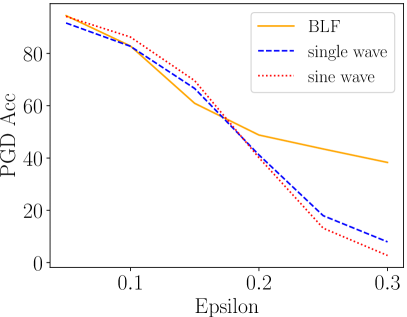
(a) MNIST Standard training

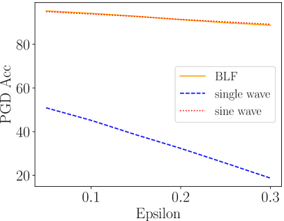
(b) MNIST Adversarial training

(c) CIFAR10 Standard training

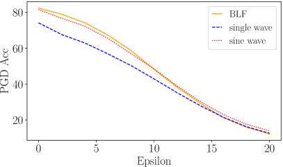
(d) CIFAR10 Adversarial training

Figure 7: Robust accuracy of 2C2F on MNIST and RN18 on CIFAR10.

In this section, we compare BLF with other bounded functions. As bounded functions, we evaluated sine wave $z=\sin(z)$ (Fig. 6 (a)) and single wave $z=\sin(z)/(\mathrm{exp}(z)+\mathrm{exp}(-z))^{2}$ (Fig. 6 (b)). We used 2C2F on MNIST and RN18 on CIFAR10 and the same experimental conditions in Section 5.2. Robust accuracies against PGD attacks are shown in Fig. 7. This figure shows that single wave is inferior to BLF, and sine wave is comparable to BLF. Note that our proposal is using bounded functions, which have finite maximum and minimum points, and not limited to using BLF. We use BLF because BLF is similar to tanh and we can evaluate the effect of finite optimal points. Even so, BLF can achieve better performance than single wave and as good performance as sine wave.

Appendix E Evaluation of input loss surface

Since Mosbach et al. (2018) have pointed out that logit regularization methods cause distorted input loss surfaces, we visualized input loss surface of each method. In this experiment, we randomly selected eight data points $\{\bm{x}^{(}i)\}_{i=1}^{8}$ from the training dataset of CIFAR10 and generated two noise vectors $\bm{v}_{1},\bm{v}_{2}$ whose elements are randomly selected from {-1, +1}. Then, we evaluated $\mathcal{L}_{CE}(\bm{x}+\varepsilon_{1}\bm{v}_{1}+\varepsilon_{2}\bm{v}_{2})$ for each dat point. $\varepsilon_{1}$ and $\varepsilon_{2}$ are noise levels, and we changed $\varepsilon_{1}$ and $\varepsilon_{2}$ from -16/255 to 16/255, in 0.5/255 increments. Note that we used the same data points and noise vectors among Baseline, logit regularization methods and TRADES. In this experiment, we used RN18 trained on CIFAR10 in the standard training and adversarial training settings.

Figures 8-11 are input loss surfaces of models trained in the standard setting, and Figures 12-16 are input loss surfaces of models trained in the adversarial setting. In the standard training setting, when we compare Baseline (Fig. 8) with logit regularization methods (Figs. 9-11), logit regularization methods seem to make the flat input space small (e.g., Data No.2, No.5, and No.6). However, we should pay attention to the scale of loss surfaces. Scales of loss surfaces for logit regularization methods are smaller than those for Baseline. For example, losses of Data No.2, No.5, and No.6 for Baseline can exceed ten by noise injection while losses for logit regularization methods are smaller than three. Thus, logit regularization methods improve the robustness against random noise. This is because logit regularization methods induce the small Lipschitz constants. Similarly, in the adversarial training settings, logit regularization methods make the amount of loss changes small, e.g., the amount of change of the loss of No.2 in Fig. 15 is smaller than the loss scale of No.2 in Fig. 12. We list the difference between the maximum loss and minimum loss ($\max_{\varepsilon_{1},\varepsilon_{2}}\mathcal{L}_{CE}(\bm{x}+\varepsilon_{1}\bm{v}_{1}+\varepsilon_{2}\bm{v}_{2})-\min_{\varepsilon_{1},\varepsilon_{2}}\mathcal{L}_{CE}(\bm{x}+\varepsilon_{1}\bm{v}_{1}+\varepsilon_{2}\bm{v}_{2})$) in Tab. 5. We can see that BLF can make the difference of losses by noise injection the smallest, and thus, BLF can improve the robustness of cross entropy loss against the random noise injection. These results support that logit regularization methods can improve the robustness against untargeted attack using cross entropy.

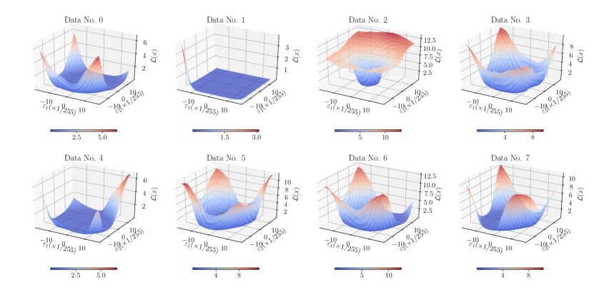
Figure 8: Loss Surface over input spaces of Baseline (standard training) on CIFAR10.

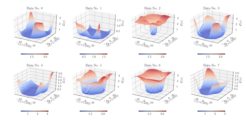
Figure 9: Loss Surface over input spaces of LSQ (standard training) on CIFAR10.

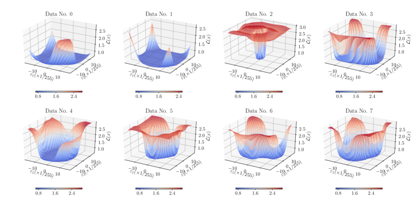
Figure 10: Loss Surface over input spaces of LSM (standard training) on CIFAR10.

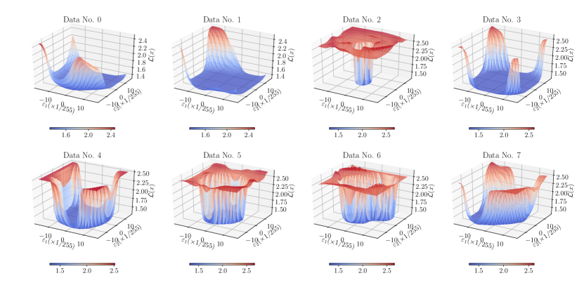
Figure 11: Loss Surface over input spaces of BLF (standard training) on CIFAR10.

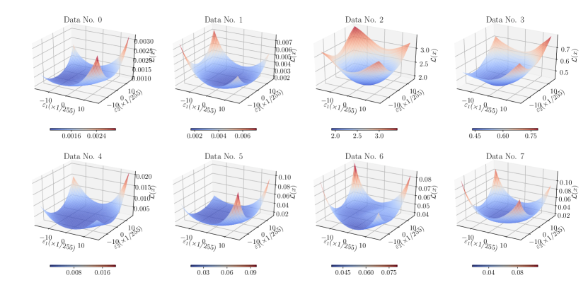
Figure 12: Loss Surface over input spaces of Baseline (adversarial training) on CIFAR10.

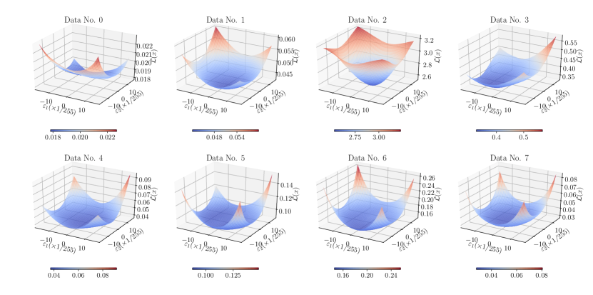
Figure 13: Loss Surface over input spaces of LSQ (adversarial training) on CIFAR10.

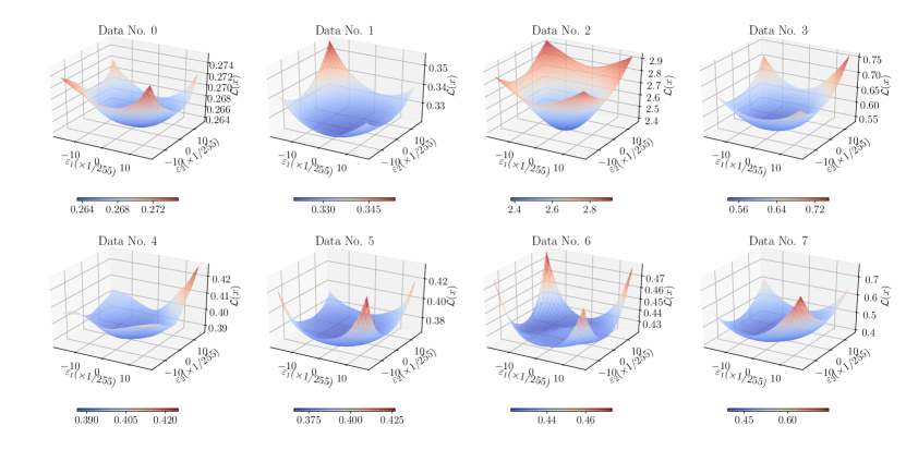
Figure 14: Loss Surface over input spaces of LSM (adversarial training) on CIFAR10.

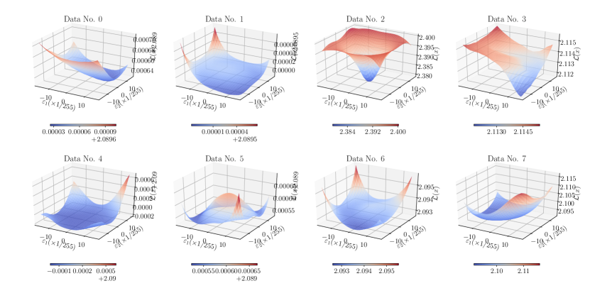
Figure 15: Loss Surface over input spaces of BLF (adversarial training) on CIFAR10.

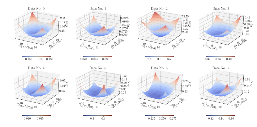
Figure 16: Loss Surface over input spaces of TRADES (adversarial training) on CIFAR10.

Table 5: The difference between the maximum loss and minimum loss for random noise in the input loss surface experiment: $\max_{\varepsilon_{1},\varepsilon_{2}}\mathcal{L}_{CE}(\bm{x}+\varepsilon_{1}\bm{v}_{1}+\varepsilon_{2}\bm{v}_{2})-\min_{\varepsilon_{1},\varepsilon_{2}}\mathcal{L}_{CE}(\bm{x}+\varepsilon_{1}\bm{v}_{1}+\varepsilon_{2}\bm{v}_{2})$ where $-16/255\leq\varepsilon_{*}\leq 16/255$. Results are averaged over eight data points.

	Baseline	LSQ	LSM	BLF	TRADES
ST	9.38	2.89	2.21	1.28	N/A
AT	0.269	0.160	0.168	0.00680	0.263

References

- Andriushchenko et al. (2020) Andriushchenko, M.; Croce, F.; Flammarion, N.; and Hein, M. 2020. Square attack: a query-efficient black-box adversarial attack via random search. In Proc. ECCV.
- Athalye, Carlini, and Wagner (2018) Athalye, A.; Carlini, N.; and Wagner, D. 2018. Obfuscated Gradients Give a False Sense of Security: Circumventing Defenses to Adversarial Examples. In Proc. ICML, 274–283.
- Carlini et al. (2019) Carlini, N.; Athalye, A.; Papernot, N.; Brendel, W.; Rauber, J.; Tsipras, D.; Goodfellow, I.; Madry, A.; and Kurakin, A. 2019. On evaluating adversarial robustness. arXiv preprint arXiv:1902.06705 .
- Carmon et al. (2019) Carmon, Y.; Raghunathan, A.; Schmidt, L.; Duchi, J. C.; and Liang, P. S. 2019. Unlabeled data improves adversarial robustness. In Proc. NeurIPS, 11190–11201.
- Cisse et al. (2017) Cisse, M.; Bojanowski, P.; Grave, E.; Dauphin, Y.; and Usunier, N. 2017. Parseval networks: Improving robustness to adversarial examples. In Proc. ICML, 854–863.
- Croce and Hein (2020) Croce, F.; and Hein, M. 2020. Reliable evaluation of adversarial robustness with an ensemble of diverse parameter-free attacks. In Proc. ICML. URL https://github.com/fra31/auto-attack.
- Ding, Wang, and Jin (2019) Ding, G. W.; Wang, L.; and Jin, X. 2019. AdverTorch v0.1: An Adversarial Robustness Toolbox based on PyTorch. arXiv preprint arXiv:1902.07623 .
- Du et al. (2019) Du, S.; Lee, J.; Li, H.; Wang, L.; and Zhai, X. 2019. Gradient descent finds global minima of deep neural networks. In Proc. ICML, 1675–1685.
- Du et al. (2018) Du, S. S.; Zhai, X.; Poczos, B.; and Singh, A. 2018. Gradient descent provably optimizes over-parameterized neural networks. arXiv preprint arXiv:1810.02054 .