Recyclable Gaussian Processes

Abstract

We present a new framework for recycling independent variational approximations to Gaussian processes. The main contribution is the construction of variational ensembles given a dictionary of fitted Gaussian processes without revisiting any subset of observations. Our framework allows for regression, classification and heterogeneous tasks, i.e. mix of continuous and discrete variables over the same input domain. We exploit infinite-dimensional integral operators based on the Kullback-Leibler divergence between stochastic processes to re-combine arbitrary amounts of variational sparse approximations with different complexity, likelihood model and location of the pseudo-inputs. Extensive results illustrate the usability of our framework in large-scale distributed experiments, also compared with the exact inference models in the literature.

1 Introduction

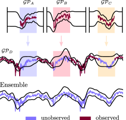
Figure 1: Recyclable GPs (A, B, C and D) are re-combined without accessing to the subsets of observations.

One of the most desirable properties for any modern machine learning method is the handling of very large datasets. Since this goal has been progressively achieved in the literature with scalable models, much attention is now paid to the notion of efficiency. For instance, in the way of accessing data. The fundamental assumption used to be that samples can be revisited without restrictions a priori. In practice, we encounter cases where the massive storage or data centralisation is not possible anymore for preserving the privacy of individuals, e.g. health and behavioral data. The mere limitation of data availability forces learning algorithms to derive new capabilities, such as i) distributing the data for federated learning (Smith et al., 2017), ii) observe streaming samples for continual learning (Goodfellow et al., 2014) and iii) limiting data exchange for private-owned models (Peterson et al., 2019).

A common theme in the previous approaches is the idea of model memorising and recycling, i.e. using the already fitted parameters in another problem or joining it with others for an additional global task without revisiting any data. If we look to the functional view of this idea, uncertainty is still much harder to be repurposed than parameters. This is the point where Gaussian process (GP) models (Rasmussen and Williams, 2006) play their role.

In this paper, we investigate a general framework for recycling distributed variational sparse approximations to GPs, illustrated in Figure 1. Based on the properties of the Kullback-Leibler divergence between stochastic processes (Matthews et al., 2016) and Bayesian inference, our method ensembles an arbitrary amount of variational GP models with different complexity, likelihood and location of pseudo-inputs, without revisiting any data.

1.1   Background.  The flexible nature of GP models for definining prior distributions over non-linear function spaces has made them a suitable alternative in many probabilistic regression and classification problems. However, GP models are not immune to settings where the model needs to adapt to irregular ways of accessing the data, e.g. asynchronous observations or missings input areas. Such settings, together with GP model’s well-known computational cost for the exact solutions, typically $\mathcal{O}(N^{3})$ where $N$ is the data size, has motivated plenty of aproaches focused on parallelising inference. Regarding the task of distributing the computational load between learning agents, GP models have been inspired by local experts (Jacobs et al., 1991, Hinton, 2002). Two seminal works exploited this connection before the modern era of GP approximations. While the Bayesian committee machine (BCM) of Tresp (2000) focused on merging independently trained GP regression models on subsets of the same data, the infinite mixture of GP experts (Rasmussen and Ghahramani, 2002) increased the model expresiveness by combining local GP experts. Our proposed method will be closer to the first approach whilst the second one is also amenable but out of the spirit of this work.

The emergence of large datasets, with size $N$$>$$10^{4}$, led to the introduction of approximate models, that in combination with variational inference (Titsias, 2009), succeed in scaling up GPs. Two more recent approaches that combine sparse GPs with ideas from distributed models or computations are Gal et al. (2014) and Deisenroth and Ng (2015). Based on the variational GP inference of Titsias (2009), Gal et al. (2014) presented a new re-parameterisation of the lower bounds that allows to distribute the computational load accross nodes, also applicable to GPs with stochastic variational inference (Hensman et al., 2013) and with non-Gaussian likelihoods (Hensman et al., 2015, Saul et al., 2016). Out of the sparse GP approach and more inspired in Tresp (2000) and product of experts (Bordley, 1982), the distributed GPs of Deisenroth and Ng (2015) scaled up the parallelisation mechanism of local experts to the range of $N$$>$$10^{6}$. Their approach is focused on exact GP regression, not considering classification or other non-Gaussian likelihoods. Table 1 provides a description of these different methods and their main properties, also if each distributed node is a GP model itself.

Table 1: Properties of distributed GP models

Model	$\mathcal{N}$ reg.	non-$\mathcal{N}$ reg.	class.	het.	inference	$\mathcal{GP}_{\textsc{node}}$	data st.
Tresp (2000)	✓	✗	✗	✗	Analytical	✓	✓
Ng and Deisenroth (2014)	✓	✗	✗	✗	Analytical	✓	✓
Cao and Fleet (2014)	✓	✗	✗	✗	Analytical	✓	✓
Deisenroth and Ng (2015)	✓	✗	✗	✗	Analytical	✓	✓
Gal et al. (2014)	✓	✓	✓	✗	Variational	✗	✗
This work	✓	✓	✓	✓	Variational	✓	✗

$(^{*})$ Respectively, Gaussian and non-Gaussian regression ($\mathcal{N}$ & non-$\mathcal{N}$ reg), classification (class), heterogeneous (het) and storage (st).

Our contribution in this paper is to provide a new framework for recycling already fitted variational approximations with the purpose of building a global GP ensemble. We use infinite-dimensional integral operators, that can be understood in the context of the Kullback-Leibler (KL) divergence between stochastic processes (Matthews et al., 2016). Here, we borrow the reparameterisation of Gal et al. (2014) to distribute the inference computation. The recyclable framework is amenable for both regression, classification and heterogeneous tasks, e.g. outputs are a mix of continuous and discrete variables. We are not restricted to any specific sparse GP approach, and several of them are suitable for combination under the ensemble GP, for instance, Hensman et al. (2013, 2015), Saul et al. (2016). We experimentally provide evidence of the performance of the recyclable GP framework in different settings and under several architectures. Our model can be viewed as an extension of Gal et al. (2014) and Deisenroth and Ng (2015) but generalised to multiple variational models without restrictions on the learning task or the likelihood distribution adopted.

2 Recyclable Gaussian Processes

We consider a supervised learning problem, where we have an input-output training dataset $\mathcal{D}=\{\bm{x}_{i},y_{i}\}^{N}_{i=1}$ with $\bm{x}\in\mathbb{R}^{p}$. We assume i.i.d. outputs $y_{i}$, that can be either continuous or discrete variables. For convenience, we will refer to the likelihood term $p(y|\bm{\theta})$ as $p(y|f)$ where the generative parameters are linked via $\bm{\theta}=f(\bm{x})$, being $f(\cdot)$ a non-linear function drawn from a zero-mean GP prior $f\sim\mathcal{GP}(\bm{0},k(\cdot,\cdot))$, and $k(\cdot,\cdot)$ is the covariance function or kernel. Importantly, when non-Gaussian outputs are considered, the GP output function $f(\cdot)$ might need an extra deterministic mapping $\Phi(\cdot)$ that transforms it to the appropriate parametric domain of $\bm{\theta}$.

The data $\mathcal{D}$ is assumed to be partitioned into an arbitrary number of $K$ subsets that we aim to observe and process independently, that is, $\{\mathcal{D}_{1},\mathcal{D}_{2},\dots,\mathcal{D}_{K}\}$. There is not any restriction on the amount of subsets or learning nodes. The subsets $\{\mathcal{D}_{k}\}_{k=1}^{K}$ do not need to have the same size, and we only restrict them to be $N_{k}$$<$$N$. However, since we treat with a huge number of observations, we still consider that $N_{k}$ for all $k\in\{1,2,\dots,K\}$ is sufficiently large for not accepting exact GP inference due to temporal and computational demand. Notice that $k$ is an index while $k(\cdot,\cdot)$ refers to the kernel.

2.1 Sparse variational approximations for distributed subsets

We adopt the sparse GP approach based on inducing variables, together with the variational framework of Titsias (2009) for the partitioned subsets. The use of auxiliary variables within approximate inference methods is widely known in the GP literature (Hensman et al., 2013, 2015, Matthews et al., 2016). In the context of $K$ distributed partitions and their adjacent samples, we define subsets of $M_{k}$$\ll$$N_{k}$ inducing inputs $\bm{Z}_{k}=\{\bm{z}_{m}\}^{M_{k}}_{m=1}$, where $\bm{z}_{m}\in\mathbb{R}^{p}$ and their non-linear function evaluations by $f(\cdot)$ are denoted as $\bm{u}_{k}=[f(\bm{z}_{1}),f(\bm{z}_{2}),\cdots,f(\bm{z}_{M_{k}})]^{\top}$. We remark that $f$ is considered to be stationary across all distributed tasks, being $\bm{u}_{k}$ $\forall k\in\{1,2,\dots,K\}$ values of the same function.

To obtain multiple independent approximations to the posterior distribution $p(f|\mathcal{D})$ of the GP function, we introduce $K$ variational distributions $q_{k}(f)$, one per distributed partition $\mathcal{D}_{k}$. In particular, each variational distribution factorises as $q_{k}(f)=p(f_{\neq\bm{u}_{k}}|\bm{u}_{k})q_{k}(\bm{u}_{k})$, with $q_{k}(\bm{u}_{k})=\mathcal{N}(\bm{u}_{k}|\bm{\mu}_{k},\bm{S}_{k})$ and $p(f_{\neq\bm{u}_{k}}|\bm{u}_{k})$ being the standard conditional GP prior distribution given the hyperparameters $\bm{\psi}_{k}$ of each $k$-th kernel. To fit the local variational distributions $q_{k}(\bm{u}_{k})$, we build lower bounds $\mathcal{L}_{k}$ on the marginal log-likelihood (ELBO) of every data partition $\mathcal{D}_{k}$. Then, we use optimisation methods, typically gradient-based, to maximise the $K$ objective functions $\mathcal{L}_{k}$, one per distributed task, separately. Each local ELBO is obtained as follows

$$\mathcal{L}_{k}=\sum_{i=1}^{N_{k}}\mathbb{E}_{q_{k}({\mathbf{f}}_{i})}\left[\log p(y_{i}|{\mathbf{f}}_{i})\right]-\text{KL}[q_{k}(\bm{u}_{k})||p_{k}(\bm{u}_{k})],$$ (1)

with $p_{k}(\bm{u}_{k})=\mathcal{N}(\bm{u}_{k}|\bm{0},{\mathbf{K}}_{kk})$, where ${\mathbf{K}}_{kk}\in\mathbb{R}^{M_{k}\times M_{k}}$ has entries $k(\bm{z}_{m},\bm{z}_{m^{\prime}})$ with $\bm{z}_{m},\bm{z}_{m^{\prime}}\in\bm{Z}_{k}$ and conditioned to certain kernel hyperparameters $\bm{\psi}_{k}$ that we also aim to optimise. The variable ${\mathbf{f}}_{i}$ corresponds to $f(\bm{x}_{i})$ and the marginal posterior comes from $q_{k}({\mathbf{f}}_{i})=\int p({\mathbf{f}}_{i}|\bm{u}_{k})q_{k}(\bm{u}_{k})d\bm{u}_{k}$. In practice, the distributed local bounds $\mathcal{L}_{k}$ are identical to the one presented in Hensman et al. (2015) and also accept stochastic variational inference (Hoffman et al., 2013, Hensman et al., 2013). An important detail is that, while the GP function is restricted to be stationary between tasks, the likelihood distribution model $p(y_{i}|f)$ is not. An example of the heterogeneous setting is shown the experiments, where we combine a Gaussian and a Bernoulli likelihood.

2.2 Global inference from local learning

Having a dictionary which contains the already fitted local variational solutions, while others can be still under computation, we focus on how using them for performing global inference of the GP. Such dictionary consists, for instance, of a list of objects $\mathcal{E}=\{\mathcal{E}_{1},\mathcal{E}_{2},\dots,\mathcal{E}_{K}\}$ without any specific order, where each $\mathcal{E}_{k}=\{\bm{\phi_{k}},\bm{\psi_{k}},\bm{Z}_{k}\}$, $\bm{\phi_{k}}$ being the corresponding variational parameters $\bm{\mu}_{k}$ and $\bm{S}_{k}$.

Ideally, to obtain a global inference solution given the GP models included in the dictionary, the resulting posterior distribution should be valid for all the local subsets of data. This is only possible if we consider the entire data set $\mathcal{D}$ in a maximum likelihood criterion setting. Specifically, our goal now is to obtain an approximate posterior $q(f)\approx p(f|\mathcal{D})$ by maximising a lower bound $\mathcal{L}_{\mathcal{E}}$ under the log-marginal likelihood $\log p(\mathcal{D})$ without revisiting the data already observed by the local models. We begin by considering the full posterior distribution of the stochastic process, similarly as Burt et al. (2019) does for obtaining an upper bound on the KL divergence. The idea is to use infinite-dimensional integral operators that were introduced by Matthews et al. (2016) in the context of variational inference, and previously by Seeger (2002) for standard GP error bounds. The use of the infinite-dimensional integrals is equivalent to an augment-and-reduce strategy (Ruiz et al., 2018). It consists of two steps: i) we augment the model to accept the conditioning on the infinite-dimensional stochastic process and ii) we use properties of Gaussian marginals to reduce the infinite-dimensional integral operators to a finite amount of GP function values of interest. Similar strategies have been used in continual learning for GPs (Bui et al., 2017, Moreno-Muñoz et al., 2019).

Global objective.  The construction considered is as follows. We first denote $\bm{y}$ as all the output targets $\{y_{i}\}^{N}_{i=1}$in the dataset $\mathcal{D}$ and $f_{\infty}$ as the augmented infinite-dimensional GP. Notice that $f_{\infty}$ contains all the function values taken by $f(\cdot)$, including that ones at $\{\bm{x}_{i}\}^{N}_{i=1}$ and $\{\bm{Z}_{k}\}^{K}_{k=1}$ for all partitions. The augmented log-marginal expression is therefore

$$\log p(\bm{y})=\log p(\bm{y}_{1},\bm{y}_{2},\dots,\bm{y}_{K})=\log\int p(\bm{y},f_{\infty})df_{\infty},$$ (2)

where each $\bm{y}_{k}=\{y_{i}\}^{N_{k}}_{i=1}$ is the subset of output values already used for training the local GP models. The joint distribution in (7) factorises according to $p(\bm{y},f_{\infty})=p(\bm{y}|f_{\infty})p(f_{\infty})$, where the l.h.s. term is the augmented likelihood distribution and the r.h.s. term would correspond to the full GP prior over the entire stochastic process. Then, we introduce a global variational distribution $q(\bm{u_{*}})=\mathcal{N}(\bm{u_{*}}|\bm{\mu_{*}},\bm{S_{*}})$ that we aim to fit by maximising a lower bound under $\log p(\bm{y})$. The variables $\bm{u_{*}}$ correspond to function values of $f(\cdot)$ given a new subset of inducing inputs $\bm{Z_{*}}=\{\bm{z}_{m}\}^{M}_{m=1}$, where $M$ is the free-complexity degree of the global variational distribution. To derive the bound, we exploit the reparameterisation introduced by Gal et al. (2014) for distributing the computational load of the expectation term. It is based in a double application of the Jensen’s inequality and obtained as

$$\log p(\bm{y})=\log\iint q(\bm{u_{*}})p(f_{\infty\neq\bm{u_{*}}}|\bm{u_{*}})p(\bm{y}|f_{\infty})\frac{p(\bm{u_{*}})}{q(\bm{u_{*}})}df_{\infty\neq\bm{u_{*}}}d\bm{u_{*}}\\ \geq\mathbb{E}_{q(\bm{u_{*}})}\left[\mathbb{E}_{p(\bm{f}_{\infty\neq\bm{u_{*}}}|\bm{u_{*}})}\left[\log p(\bm{y}|f_{\infty})\right]+\log\frac{p(\bm{u_{*}})}{q(\bm{u_{*}})}\right],$$ (3)

where we applied the properties of Gaussian conditionals to factorise the GP prior as $p(f_{\infty})=p(\bm{f}_{\infty\neq\bm{u_{*}}}|\bm{u_{*}})p(\bm{u_{*}})$. Here, the last prior distribution is $p(\bm{u_{*}})=\mathcal{N}(\bm{u_{*}}|\bm{0},{\mathbf{K}}_{\bm{**}})$ where $\left[{\mathbf{K}}_{\bm{**}}\right]_{m,n}:=k(\bm{z}_{m},\bm{z}_{n})$, with $\bm{z}_{m},\bm{z}_{n}\in\bm{Z_{*}}$, conditioned to the global kernel hyperparameters $\bm{\psi_{*}}$ that we also aim to estimate. The double expectation in (3) comes from the factorization of the infinite-dimensional integral operator and the application of the Jensen’s inequality twice. Its derivation is in the appendix.

Local likelihood reconstruction.  The augmented likelihood distribution is perhaps, the most important point of the derivation. It allows us to apply conditional independence (CI) between the subsets of distributed output targets. This gives a factorized term that we will later use for introducing the local variational experts in the bound, that is, $\log p(\bm{y}|f_{\infty})=\sum_{k=1}^{K}\log p(\bm{y}_{k}|f_{\infty})$. To avoid revisiting local likelihood terms, and hence, evaluating distributed subsets of data that might not be available, we use the Bayes theorem but conditioned to the infinite-dimensional augmentation. It indicates that the local variational distributions can be approximated as

$$q_{k}(f_{\infty})\approx p(f_{\infty}|\bm{y}_{k})\propto p(f_{\infty})p(\bm{y}_{k}|f_{\infty}),$$ (4)

where the augmented approximate distribution factorises as $q_{k}(f_{\infty})=p(f_{\infty\neq\bm{u}_{k}}|\bm{u}_{k})q_{k}(\bm{u}_{k})$ as in the variational framework of Titsias (2009). Similar expressions consisting on the full stochastic process conditionals were previously used in Bui et al. (2017) and Matthews et al. (2016), with emphasis on the theoretical consistency of augmentation. Thus, we can find an approximation for each local likelihood term $p(\bm{y}_{k}|f_{\infty})$ by inverting the Bayes theorem in (4). Then, the conditional expectation in (3) turns to be

$$\mathbb{E}_{p(\bm{f}_{\infty\neq\bm{u_{*}}}|\bm{u_{*}})}\left[\log p(\bm{y}|f_{\infty})\right]\approx\sum_{k=1}^{K}\mathbb{E}_{p(\bm{f}_{\infty\neq\bm{u_{*}}}|\bm{u_{*}})}\left[\log\frac{q_{k}(f_{\infty})}{p(f_{\infty})}\right]=\sum_{k=1}^{K}\mathbb{E}_{p(\bm{u}_{k}|\bm{u_{*}})}\left[\log\frac{q_{k}(\bm{u}_{k})}{p(\bm{u}_{k})}\right],$$

where we applied properties of Gaussian marginals to reduce the infinite-dimensional expectation, and factorised the distributions to be explicit on each subset of fixed inducing-variables $\bm{u}_{k}$ rather than $f_{\infty}$. For instance, the integral $\int p(f_{\infty})d\bm{f}_{\infty\neq\bm{u}_{k}}$ is analogous to $\int p(\bm{f}_{\infty\neq\bm{u}_{k}},\bm{u}_{k})d\bm{f}_{\infty\neq\bm{u}_{k}}=p(\bm{u}_{k})$ via marginalisation.

Variational contrastive expectations.  The introduction of $K$ expectation terms over the log-ratios in the bound of (3) as a substitution of the local likelihoods, leads to particular advantages. If we have a nested integration in (3), first over $\bm{u_{*}}$ at the conditional prior distribution, and second over $\bm{u}_{k}$ given the log-ratio $q_{k}(\bm{u}_{k})/p(\bm{u}_{k})$, we can exploit the GP predictive equation to write down

$$\sum_{k=1}^{K}\mathbb{E}_{q(\bm{u_{*}})}\left[\mathbb{E}_{p(\bm{u}_{k}|\bm{u_{*}})}\left[\log\frac{q_{k}(\bm{u}_{k})}{p(\bm{u}_{k})}\right]\right]=\sum_{k=1}^{K}\mathbb{E}_{q_{\mathcal{C}}(\bm{u}_{k})}\left[\log\frac{q_{k}(\bm{u}_{k})}{p(\bm{u}_{k})}\right],$$ (5)

where we obtained $q_{\mathcal{C}}(\bm{u}_{k})$ via the integral $q_{\mathcal{C}}(\bm{u}_{k})=\int q(\bm{u_{*}})p(\bm{u}_{k}|\bm{u_{*}})d\bm{u_{*}}$, that coincides with the approximate predictive GP posterior. This distribution can be obtained analytically for each $k$-th subset $\bm{u}_{k}$ using the following expression, whose complete derivation is provided in the appendix,

$$q_{\mathcal{C}}(\bm{u}_{k})=\mathcal{N}(\bm{u}_{k}|{\mathbf{K}}_{\bm{*}k}^{\top}{\mathbf{K}}_{\bm{**}}^{-1}\bm{\mu_{*}},{\mathbf{K}}_{kk}+{\mathbf{K}}_{\bm{*}k}^{\top}{\mathbf{K}}_{\bm{**}}^{-1}(\bm{S_{*}}-{\mathbf{K}}_{\bm{**}}){\mathbf{K}}_{\bm{**}}^{-1}{\mathbf{K}}_{\bm{*}k}),$$

where, once again, $\bm{\phi_{*}}=\{\bm{\mu_{*}},\bm{S_{*}}\}$ are the global variational parameters that we aim to learn. One important detail of the sum of expectations in (16) is that it works as an average contrastive indicator that measures how well the global $q(\bm{u_{*}})$ is being fitted to the local experts $q_{k}(\bm{u}_{k})$. Without the need of revisiting any distributed subset of data samples, the GP predictive $q_{\mathcal{C}}(\bm{u}_{k})$ is playing a different role in contrast with the usual one. Typically, we assume the approximate posterior fixed and fitted, and we evaluate its performance on some test data points. In this case, it goes in the opposite way, the approximate variational distribution is unfixed, and it is instead evaluated over each $k$-th local subset of inducing-inputs $\bm{Z}_{k}$.

Lower ensemble bounds.  We are now able to simplify the initial bound in (3) by substituting the first term with the contrastive expectations presented in (16). This substitution gives the final version of the lower bound $\mathcal{L}_{\mathcal{E}}\leq\log p(\bm{y})$ on the log-marginal likelihood for the global GP,

$$\mathcal{L}_{\mathcal{E}}=\sum_{k=1}^{K}\mathbb{E}_{q_{\mathcal{C}}(\bm{u}_{k})}\left[\log q_{k}(\bm{u}_{k})-\log p(\bm{u}_{k})\right]-\text{KL}\left[q(\bm{u_{*}})||p(\bm{u_{*}})\right].$$ (6)

The maximisation of (6) is w.r.t. the parameters $\bm{\phi_{*}}$, the hyperparameters $\bm{\psi_{*}}$ and $\bm{Z_{*}}$. To assure the positive-definitiness of variational covariance matrices $\{\bm{S}_{k}\}^{K}_{k=1}$ and $\bm{S_{*}}$ on both local and global cases, we consider that they all factorize according to the Cholesky decomposition $\bm{S}={\mathbf{L}}{\mathbf{L}}^{\top}$. We can then use unconstrained optimization to find optimal values for the lower-triangular matrices ${\mathbf{L}}$.

A priori, the ensemble GP bound is agnostic with respect to the likelihood model. There is a general derivation in Matthews et al. (2016) of how stochastic processes and their integral operators are affected by projection functions, that is, different linking mappings of the function $f(\cdot)$ to the parameters $\bm{\theta}$. In such cases, the local lower bounds $\mathcal{L}_{k}$ in (1) might include expectation terms that are intractable. Since we build the framework to accept any possible data-type, we propose to solve the integrals via Gaussian-Hermite quadratures as in Hensman et al. (2015), Saul et al. (2016) and if this is not possible, an alternative would be to apply Monte-Carlo methods.

Computational cost and connections.  The computational cost of the local models is $\mathcal{O}(N_{k}M_{k}^{2})$, while the global GP reduces to $\mathcal{O}((\sum_{k}M_{k})M^{2})$ and $\mathcal{O}(M^{2})$ in training and prediction, respectively. The methods in Table 1 typically need $\mathcal{O}(\sum_{k}N_{k}^{2})$ for global prediction. A last theoretical aspect is the link between the global bound in (6) and the underlying idea in Tresp (2000), Deisenroth and Ng (2015). Distributed GP models are based on the application of CI to factorise the likelihood terms of subsets. To approximate the posterior predictive, they combine local estimates, divided by the GP prior. It is analogous to (6), but in the logarithmic plane and the variational inference setup.

2.3 Capabilities of recyclable GPs

We highlight several use cases for the proposed framework. The idea of recycling GP models opens the door to multiple extensions, with particular attention to the local-global modelling of heterogeneous data problems and the adaptation of model complexity in a data-driven manner.

Global prediction.  Our purpose might be to predict how likely an output test datum $y_{t}$ is at some point $\bm{x}_{t}$ of the input space $\mathbb{R}^{p}$. In this case, the global predictive distribution can be approximated as $p(y_{t}|\mathcal{D})\approx\int p(y_{t}|{\mathbf{f}}_{t})q({\mathbf{f}}_{t})d{\mathbf{f}}_{t}$, with $q({\mathbf{f}}_{t})=\int p({\mathbf{f}}_{t}|\bm{u_{*}})q(\bm{u_{*}})d\bm{u_{*}}$. As mentioned in the previous subsection, the integral can be obtained by quadratures when the solution is intractable.

Heterogeneous single-output GP.  Extensions to GPs with heterogeneous likelihoods, that is, a mix of continuous and discrete variables $\bm{y}_{i}$, have been proposed for multi-output GPs (Moreno-Muñoz et al., 2018). However, there are no restrictions in our single-output model to accept different likelihoods $p(y_{i}|f(\bm{x}_{i}))$ per data point $\{\bm{x}_{i},y_{i}\}$. An inconvenience of the bound in (1), is that, each $i$-th expectation term could be imbalanced with respect to the others. For example, if mixing Bernoulli and Gaussian variables, binary outputs could contribute more to the objective function than the rest, due to the dimensionality. To overcome this issue, we fit a local GP model to each heterogeneous variable. We join all models together using the ensemble bound in (6) to propagate the uncertainty in a principled way. Although, data-types need to be known beforehand, perhaps as additional labels.

Recyclable GPs and new data.  In practice, it might not be necessary to distribute the whole dataset $\mathcal{D}$ in parallel tasks, with some subsets $\mathcal{D}_{k}$ available at the global ensemble. It is possible to combine the samples in $\mathcal{D}_{k}$ with the dictionary of local GP variational distributions. In such cases, we would only approximate the likelihood terms in (3) related to the distributed subsets of samples. The resulting combined bound would be equivalent to (6) with an additional expectation term on the new data. We provide the derivation of this combined bound in the supplementary material.

Stationarity and expressiveness.  We assume that the non-linear function $f$ is stationary across subsets of data. If this assumption is relaxed, some form of adaptation or forgetting should be included to match the local GPs. Other types of models can be considered for the ensemble, as for instance, with several latent functions (Lázaro-Gredilla and Titsias, 2011) or sparse multi-output GPs (Álvarez and Lawrence, 2011). The model also accepts GPs with increased expressiveness. For example, to get multi-modal likelihoods, we can use mixture of GP experts (Rasmussen and Ghahramani, 2002).

Data-driven complexity and recyclable ensembles.  One of the main advantages of the recyclable GP framework is that it allows data-driven updates of the complexity. That is, if an ensemble ends in a new variational GP model, it also can be recycled. Hence, the number of global inducing-variables $M$ can be iteratively increased conditioned to the amount of samples considered. A similar idea was already commented as an application of the sparse order-selection theorems by Burt et al. (2019).

Model recycling and use cases.  The ability of recycling GPs in future global tasks have a significant impact in behavioral applications, where fitted private-owned models in smartphones can be shared for global predictions rather than data. Its application to medicine is also of high interest. If one has personalized GPs for patients, epidemiologic surveys can be built without centralising private data.

3 Related Work

In terms of distributed inference for scaling up computation, that is, the delivery of calculus operations across parallel nodes but not data or independent models, we are similar to Gal et al. (2014). Their approach can be understood as a specific case of our framework. Alternatively, if we look to the property of having nodes that contain usable GP models (Table 1), we are similar to Deisenroth and Ng (2015), Cao and Fleet (2014) and Tresp (2000), with the difference that we introduce variational approximation methods for non-Gaussian likelihoods. An important detail is that the idea of exploiting properties of full stochastic processes (Matthews et al., 2016) for substituting likelihood terms in a general bound has been previously considered in Bui et al. (2017) and Moreno-Muñoz et al. (2019). Whilst the work of Bui et al. (2017) ends in the derivation of expectation-propagation (EP) methods for streaming inference in GPs, the introduction of the reparameterisation of Gal et al. (2014) makes our inference and performance different from Moreno-Muñoz et al. (2019). There is also the inference framework of Bui et al. (2018) for both federated and continual learning, but focused on EP and the Bayesian approach of Nguyen et al. (2018). A short analysis of its application to GPs is included for continual learning settings but far from the large-scale scope of our paper. Moreover, the spirit of using inducing-points as pseudo-approximations of local subsets of data is shared with Bui and Turner (2014), that comments its potential application to distributed setups. More oriented to dynamical modular models, we find the work by Velychko et al. (2018), whose factorisation across tasks is similar to Ng and Deisenroth (2014) but oriented to state-space models.

4 Experiments

In this section, we evaluate the performance of our framework for multiple recyclable GP models and data access settings. To illustrate its usability, we present results in three different learning scenarios: i) regression, ii) classification and iii) heterogeneous data. All experiments are numbered from one to nine in roman characters. Performance metrics are given in terms of the negative log-predictive density (nlpd), root mean square error (rmse) and mean-absolute error (mae). We provide Pytorch code that allows to easily learn the GP ensembles. It also includes the baseline methods. The syntax follows the spirit of providing a list of  recyclable_models = [$\texttt{GP}_{1}$, $\texttt{GP}_{2}$, $\texttt{GP}_{3}$], where each $\texttt{GP}_{k}$ contains exclusively parameters of the local approximations. Further details about initialization, optimization and metrics are in the appendix. Importantly, we remark that data is never revisited and its presence in the ensemble plots is just for clarity in the comprehension of results.

4.1   Regression.  In our first experiments for variational GP regression with distributed models, we provide both qualitative and quantitative results about the performance of recyclable ensembles. (i) Toy concatenation: In Figure 2, we show three of five tasks united in a new GP model. Tasks are GPs fitted independently with $N_{k}$$=$$500$ synthetic data points and $M_{k}$$=$$15$ inducing variables per distributed task. The ensemble fits a global variational solution of dimension $M$$=$$35$. Notice that the global variational GP tends to match the uncertainty of the local approximations. (ii) Distributed GPs: We provide error metrics for the recyclable GP framework compared with the state-of-the-art models in Table 3. The training data is synthetic and generated as a combination of $\sin(\cdot)$ functions (in the appendix). For the case with 10k observations, we used $K$$=$$50$ tasks with $N_{k}$$=$$200$ data-points and $M_{k}$$=$$3$ inducing variables in the sparse GP. The scenario for 100k is similar but divided into $K$$=$$250$ tasks with $N_{k}$$=$$400$. Our method obtains better results than the exact distributed solutions due to the ensemble bound searches the average solution among all recyclable GPs. The baseline methods are based on a combination of solutions, if one is bad-fitted, it has a direct effect on the predictive performance. We also tested the data with the inference setup of Gal et al. (2014), obtaining an nlpd of $2.58\pm 0.11$ with $250$ nodes for 100k data. It is better than ours and the baseline methods, but without a GP reconstruction, only distributes the computation of matrix terms. (iii) Recyclable ensembles: For a large synthetic dataset ($N$$=$$10^{6}$), we tested the recyclable GPs with $K$$=$$5\cdot 10^{3}$ tasks as shown in Table 3. However, if we ensemble large amount of local GPs, e.g. $K$$\gg$$10^{3}$, it is problematic for baseline methods, due to partitions must be revisited for building predictions and if one-of-many GP fails, performance decreases. Then, we repeated the experiment in a pyramidal way. That is, building ensembles of recyclable ensembles, inspired in Deisenroth and Ng (2015). Our method obtained $\{\textsc{nlpd}$$=$$4.15,\textsc{rmse}$$=$$2.71$$,\textsc{mae}$$=$$2.27\}$. The results in Table 3 indicate that our model is more robust under the concatenation of approximations rather than overlapping them in the input space. (iv) Solar physics dataset: We tested the framework on solar data (available at https://solarscience.msfc.nasa.gov/), which consists of more than $N$$=$$10^{3}$ monthly average estimates of the sunspot counting numbers from 1700 to 1995. We applied the mapping $\log(1+y_{i})$ to the output targets for performing Gaussian regression. Metrics are provided in Table 2, where std. values were small, so we do not include them. The perfomance with $50$ tasks is close to the baseline solutions, but without storing all distributed subsets of data.

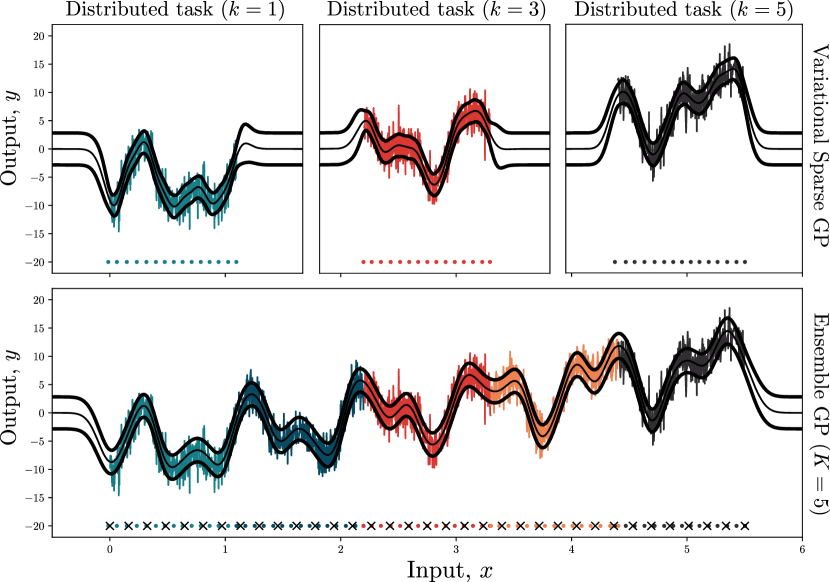
Figure 2: Recyclable GPs with synthetic data.

Table 2: Performance metrics for distributed GP regression with the solar physics dataset. (std. $\times 10^{2}$)

Model	nlpd	rmse
BCM	$-$	$17.25$
PoE	$1.51\pm 0.01$	$1.08$
GPoE	$1.51\pm 0.07$	$1.08$
RBCM	$1.53\pm 0.01$	$1.11$
This work	$1.68\pm 0.14$	$1.17\pm 0.12$

Table 3: Comparative error metrics for distributed GP models

Data size $\rightarrow$		10k			100k			1m
Model	nlpd	rmse	mae	nlpd	rmse	mae	nlpd	rmse	mae
BCM	$2.99\pm 0.94$	$11.94\pm 18.89$	$2.05\pm 1.31$	$3.51\pm 0.73$	$2.33\pm 0.96$	$1.34\pm 1.03$	na	$9.56\pm 14.87$	$1.19\pm 0.86$
PoE	$2.79\pm 0.16$	$2.32\pm 0.22$	$1.86\pm 0.22$	$2.82\pm 0.67$	$2.19\pm 0.91$	$1.71\pm 0.84$	$2.91\pm 0.63$	$1.98\pm 0.61$	$1.32\pm 0.05$
GPoE	$2.79\pm 0.56$	$2.43\pm 0.52$	$1.96\pm 0.48$	${\color[rgb]{1,0,0}\mathbf{2.73}\pm\mathbf{0.72}}$	$2.19\pm 0.91$	$1.71\pm 0.84$	$2.72\pm 0.52$	$1.98\pm 0.61$	$\mathbf{1.32}\pm\mathbf{0.05}$
RBCM	$2.96\pm 0.51$	$2.49\pm 0.51$	$2.02\pm 0.46$	$3.03\pm 0.86$	$2.51\pm 1.12$	$1.99\pm 1.04$	$\mathbf{2.56}\pm\mathbf{0.06}$	$\mathbf{1.82}\pm\mathbf{0.02}$	$1.37\pm 0.03$
This work	${\color[rgb]{0,0,1}\mathbf{2.71}\pm\mathbf{0.11}}$	${\color[rgb]{0,0,1}\mathbf{1.56}\pm\mathbf{0.04}}$	${\color[rgb]{0,0,1}\mathbf{0.97}\pm\mathbf{0.05}}$	$2.89\pm 0.07$	${\color[rgb]{1,0,0}\mathbf{1.73}\pm\mathbf{0.01}}$	${\color[rgb]{1,0,0}\mathbf{1.23}\pm\mathbf{0.02}}$	$2.87\pm 0.09$	$1.87\pm 0.07$	$1.34\pm 0.09$

Acronyms: BCM (Tresp, 2000), PoE (Ng and Deisenroth, 2014), GPoE (Cao and Fleet, 2014) and RBCM (Deisenroth and Ng, 2015).

4.2   Classification.  We adapted the entire recyclable GP framework to accept non-Gaussian likelihoods, and in particular, binary classification with Bernoulli distributions. We use the sigmoid mapping to link the GP function and the probit parameters. (iv) Pixel-wise MNIST classification: Inspired in the MNIST $\{0,1\}$ experiments of Van der Wilk et al. (2017), we threshold images of zeros and ones to black and white pixels. Then, to simulate a pixel-wise learning scenario, we used each pixel as an input-output datum whose input $\bm{x}_{i}$ contains the two coordinates ($x_{1}$ and $x_{2}$ axes). Plots in Figure 4 illustrate that a predictive ensemble can be built from smaller pieces of GP models, four corners in the case of the number zero and two for the number one. (v) Compositional number: As an illustration of potential applications of the recyclable GP approach, we build a number eight predictor using exclusively two subsets of the approximations learned in the previous experiment with the image of a zero. The trick is to shift $\bm{Z}_{k}$ to place the local approximations in the desired position. (vi) Banana dataset: We used the popular dataset in sparse GP classification for testing our method with $M$$=$$25$. We obtained a test nlpd$=7.21\pm 0.04$, while the baseline variational GP test nlpd was $7.29\pm 7.85$$\times$$10^{-4}$. The improvement is understandable as the total number of inducing points, including the local ones, is higher in the recyclable GP scenario.

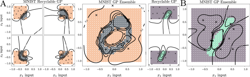
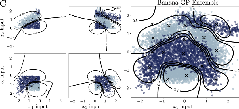
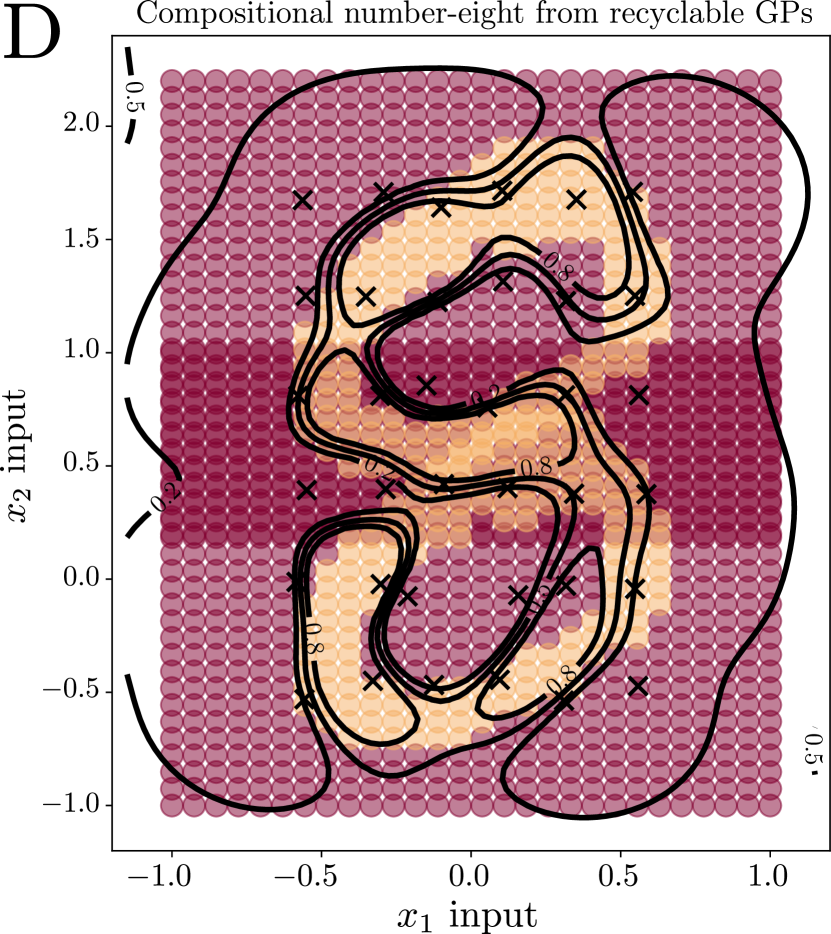
Figure 4: Recyclable GPs for $\{0,1\}$ MNIST (A-B), banana (C) and compositional number eight (D) experiments.

4.3   Heterogeneous tasks.  We analysed how ensembles of recyclable GPs can be used if one of the local tasks is regression and the other a GP classifier. (viii) London household data: We have two subsets of input-output variables: the binary contract of houses (leasehold vs. freehold) and the price per latitude-longitude coordinate in the London area. Three quadrants (Q) of the city $\{$Q2, Q3, Q4$\}$ are trained with a GP classifier and Q1 as regression. To clarify, Q1 is the right-upper corner given the central axes. Our purpose is to combine the local latent $\bm{u}_{k}$, learned with the binary data on $\{$Q2, Q3, Q4$\}$ and the $\bm{u}_{k}$ learned on Q1 via regression. Then, we search the global $f$ to be predict with a Bernoulli likelihood in Q1. The ensemble shows a test nlpd of $7.94\pm 0.01$ in classification while the recyclable task predicts with an nlpd of $8.00\pm 0.01$ in the Q1. We asses that the heterogeneous GP prediction is better in Q1 than the local GP classifier. The mean GP of regression is passed through the sigmoid function to show the multimodality.

5 Conclusion

We introduced a novel framework for building global approximations from already fitted GP models. Our main contribution is the construction of ensemble bounds that accept parameters from regression, classification and heterogeneous GPs with different complexity without revisiting any data. We analysed its performance on synthetic and real data with different structure and likelihood models. Experimental results show evidence that the method is robust. In future work, it would be interesting to extend the framework to include convolutional kernels (Van der Wilk et al., 2017) for image processing and functional regularisation (Titsias et al., 2020) for continual learning applications.

Acknowledgements

This work was supported by the Ministerio de Ciencia, Innovación y Universidades under grant TEC2017-92552-EXP (aMBITION), by the Ministerio de Ciencia, Innovación y Universidades, jointly with the European Commission (ERDF), under grants TEC2017-86921-C2-2-R (CAIMAN) and RTI2018-099655-B-I00 (CLARA), and by the Comunidad de Madrid under grant Y2018/TCS-4705 (PRACTICO-CM). PMM acknowledges the support of his FPI grant BES-2016-077626 from the Ministerio of Economía of Spain. MAA has been financed by the EPSRC Research Projects EP/R034303/1 and EP/T00343X/1. MAA has also been supported by the Rosetrees Trust (ref: A2501).

Appendix A.  Detailed Derivation of the Lower Ensemble Bound

The construction of ensemble variational bounds from recyclable GP models is based on the idea of augmenting the marginal likelihood to be conditioned on the infinite-dimensional GP function $f_{\infty}$. Notice that $f_{\infty}$ contains all the function values taken by $f(\cdot)$ over the input-space $\mathbb{R}^{p}$, including the input targets $\{\bm{x}_{i}\}^{N}_{i=1}$, the local inducing-inputs $\{\bm{Z}_{k}\}^{K}_{k=1}$ and the global ones $\bm{Z}_{*}$. Having $K$ partitions of the dataset $\mathcal{D}$ with their corresponding outputs $\bm{y}=\{\bm{y}_{1},\bm{y}_{2},\dots,\bm{y}_{K}\}$, we begin by augmenting the marginal log-likelihood as

$$\log p(\bm{y})=\log p(\bm{y}_{1},\bm{y}_{2},\dots,\bm{y}_{K})=\log\int p(\bm{y},f_{\infty})df_{\infty},$$ (7)

that factorises according to

$$\log\int p(\bm{y},f_{\infty})df_{\infty}=\log\int p(\bm{y}|f_{\infty})p(f_{\infty})df_{\infty},$$ (8)

where $p(\bm{y}|f_{\infty})$ is the augmented likelihood term of all the output targets of interest and $p(f_{\infty})$ the GP prior over the infinite amount of points in the input-space $\mathbb{R}^{p}$. This last distribution takes the form of an infinite-dimensional Gaussian, that we avoid to evaluate explicitly in the equations. To build the lower bound on the log-marginal likelihood, we first introduce the global variational distribution $q(\bm{u_{*}})=\mathcal{N}(\bm{u_{*}}|\bm{\mu_{*}},\bm{S_{*}})$ into the equation,

$$\log p(\bm{y})=\log\int p(\bm{y}|f_{\infty})p(f_{\infty})df_{\infty}=\log\int\frac{q(\bm{u_{*}})}{q(\bm{u_{*}})}p(\bm{y}|f_{\infty})p(f_{\infty})df_{\infty}\\ =\log\iint\frac{q(\bm{u_{*}})}{q(\bm{u_{*}})}p(\bm{y}|f_{\infty})p(f_{\infty\neq\bm{u_{*}}}|\bm{u_{*}})p(\bm{u_{*}})df_{\infty\neq\bm{u_{*}}}d\bm{u_{*}}.$$ (9)

Notice that the differentials $df_{\infty}$ have been splitted into $df_{\infty\neq\bm{u_{*}}}d\bm{u_{*}}$, and at the same time, we applied properties of Gaussian conditionals in the GP prior to rewrite $p(f_{\infty})$ as $p(f_{\infty\neq\bm{u_{*}}}|\bm{u_{*}})p(\bm{u_{*}})$. When the target variables $\bm{u_{*}}$ are explicit in the expression, our second step is the application of the Jensen inequality twice as it is done in the reparameterisation of (Gal et al., 2014), that is

$$\log p(\bm{y})=\log\iint\frac{q(\bm{u_{*}})}{q(\bm{u_{*}})}p(\bm{y}|f_{\infty})p(f_{\infty\neq\bm{u_{*}}}|\bm{u_{*}})p(\bm{u_{*}})df_{\infty\neq\bm{u_{*}}}d\bm{u_{*}}\\ =\log\iint q(\bm{u_{*}})p(f_{\infty\neq\bm{u_{*}}}|\bm{u_{*}})p(\bm{y}|f_{\infty})\frac{p(\bm{u_{*}})}{q(\bm{u_{*}})}df_{\infty\neq\bm{u_{*}}}d\bm{u_{*}}\\ =\log\left(\mathbb{E}_{q(\bm{u}_{*})}\left[\mathbb{E}_{p(\bm{f}_{\infty\neq\bm{u}_{*}}|\bm{u}_{*})}\left[p(\bm{y}|f_{\infty})\frac{p(\bm{u_{*}})}{q(\bm{u_{*}})}\right]\right]\right)\\ \geq\mathbb{E}_{q(\bm{u}_{*})}\left[\log\left(\mathbb{E}_{p(\bm{f}_{\infty\neq\bm{u}_{*}}|\bm{u}_{*})}\left[p(\bm{y}|f_{\infty})\frac{p(\bm{u_{*}})}{q(\bm{u_{*}})}\right]\right)\right]\\ \geq\mathbb{E}_{q(\bm{u}_{*})}\left[\mathbb{E}_{p(\bm{f}_{\infty\neq\bm{u}_{*}}|\bm{u}_{*})}\left[\log\left(p(\bm{y}|f_{\infty})\frac{p(\bm{u_{*}})}{q(\bm{u_{*}})}\right)\right]\right]=\mathcal{L}_{\mathcal{E}}.$$ (10)

Then, if we have (10), which is the first version of our ensemble lower bound $\mathcal{L}_{\mathcal{E}}$, we can use the augmented likelihood term $p(\bm{y}|f_{\infty})$ to introduce the local approximations to $f$ instead of revisiting the data. This is,

$$\mathcal{L}_{\mathcal{E}}=\mathbb{E}_{q(\bm{u}_{*})}\left[\mathbb{E}_{p(\bm{f}_{\infty\neq\bm{u}_{*}}|\bm{u}_{*})}\left[\log p(\bm{y}|f_{\infty})+\log\left(\frac{p(\bm{u_{*}})}{q(\bm{u_{*}})}\right)\right]\right]\\ =\mathbb{E}_{q(\bm{u}_{*})}\left[\mathbb{E}_{p(\bm{f}_{\infty\neq\bm{u}_{*}}|\bm{u}_{*})}\left[\log p(\bm{y}|f_{\infty})\right]-\log\left(\frac{q(\bm{u_{*}})}{p(\bm{u_{*}})}\right)\right]\\ =\mathbb{E}_{q(\bm{u}_{*})}\left[\mathbb{E}_{p(\bm{f}_{\infty\neq\bm{u}_{*}}|\bm{u}_{*})}\left[\sum^{K}_{k=1}\log p(\bm{y}_{k}|f_{\infty})\right]-\log\left(\frac{q(\bm{u_{*}})}{p(\bm{u_{*}})}\right)\right]\\ =\mathbb{E}_{q(\bm{u}_{*})}\left[\sum^{K}_{k=1}\mathbb{E}_{p(\bm{f}_{\infty\neq\bm{u}_{*}}|\bm{u}_{*})}\left[\log p(\bm{y}_{k}|f_{\infty})\right]-\log\left(\frac{q(\bm{u_{*}})}{p(\bm{u_{*}})}\right)\right],$$ (11)

where the log-ratio $q(\bm{u_{*}})/p(\bm{u_{*}})$ acts as a constant to the second expectation $\mathbb{E}_{p(\bm{f}_{\infty\neq\bm{u}_{*}}|\bm{u}_{*})}\left[\cdot\right]$ and we applied conditional independence (CI) among all the output partitions given the latent function $f_{\infty}$. That is, we introduced $p(\bm{y}|f_{\infty})=\prod^{K}_{k=1}p(\bm{y}_{k}|f_{\infty})$ to factorise the expectation term in (11) across the $K$ tasks.

Under the approximation of $p(\bm{y}_{k}|f_{\infty})$ obtained by inverting the Bayes theorem, we use $p(\bm{y}_{k}|f_{\infty})\approx q_{k}(f_{\infty})/p_{k}(f_{\infty})$ to introduce the local posterior distributions $q_{k}(\cdot)$ and priors $p_{k}(\cdot)$ in the bound $\mathcal{L}_{\mathcal{E}}$. This leads to

$$\mathcal{L}_{\mathcal{E}}=\mathbb{E}_{q(\bm{u}_{*})}\left[\sum^{K}_{k=1}\mathbb{E}_{p(\bm{f}_{\infty\neq\bm{u}_{*}}|\bm{u}_{*})}\left[\log p(\bm{y}_{k}|f_{\infty})\right]-\log\left(\frac{q(\bm{u_{*}})}{p(\bm{u_{*}})}\right)\right]\\ \approx\mathbb{E}_{q(\bm{u}_{*})}\left[\sum^{K}_{k=1}\mathbb{E}_{p(\bm{f}_{\infty\neq\bm{u}_{*}}|\bm{u}_{*})}\left[\log\left(\frac{q_{k}(f_{\infty})}{p_{k}(f_{\infty})}\right)\right]-\log\left(\frac{q(\bm{u_{*}})}{p(\bm{u_{*}})}\right)\right]\\ =\mathbb{E}_{q(\bm{u}_{*})}\left[\sum^{K}_{k=1}\mathbb{E}_{p(\bm{f}_{\infty\neq\bm{u}_{*}}|\bm{u}_{*})}\left[\log\left(\frac{\cancel{p(\bm{f}_{\infty\neq\bm{u}_{k}}|\bm{u}_{k})}q_{k}(\bm{u}_{k})}{\cancel{p(\bm{f}_{\infty\neq\bm{u}_{k}}|\bm{u}_{k})}p_{k}(\bm{u}_{k})}\right)\right]-\log\left(\frac{q(\bm{u_{*}})}{p(\bm{u_{*}})}\right)\right]\\ =\mathbb{E}_{q(\bm{u}_{*})}\left[\sum^{K}_{k=1}\mathbb{E}_{p(\bm{f}_{\infty\neq\bm{u}_{*}}|\bm{u}_{*})}\left[\log\left(\frac{q_{k}(\bm{u}_{k})}{p_{k}(\bm{u}_{k})}\right)\right]-\log\left(\frac{q(\bm{u_{*}})}{p(\bm{u_{*}})}\right)\right],$$ (12)

where we now have the explicit local distributions $q_{k}(\bm{u}_{k})$ and $p_{k}(\bm{u}_{k})$ on the subsets of inducing-inputs $\{\bm{Z}_{k}\}^{K}_{k=1}$. The cancellation of conditionals is a result of the variational factorization (Titsias, 2009). Looking to the last version of the bound in (12), there is still one point that maintains the infinite-dimensionality, the conditional prior $p(\bm{f}_{\infty\neq\bm{u}_{*}}|\bm{u}_{*})$ and its corresponding expectation term $\mathbb{E}_{p(\bm{f}_{\infty\neq\bm{u}_{*}}|\bm{u}_{*})}\left[\cdot\right]$. To adapt it to the local inducing variables $\bm{u}_{k}$, we apply the following simplification to each $k$-th integral in (12) based in the properties of Gaussian marginals (see section A.1),

$$\mathbb{E}_{p(\bm{f}_{\infty\neq\bm{u}_{*}}|\bm{u}_{*})}\left[\log\left(\frac{q_{k}(\bm{u}_{k})}{p_{k}(\bm{u}_{k})}\right)\right]=\int p(\bm{f}_{\infty\neq\bm{u}_{*}}|\bm{u}_{*})\log\left(\frac{q_{k}(\bm{u}_{k})}{p_{k}(\bm{u}_{k})}\right)d\bm{f}_{\infty\neq\bm{u}_{*}}\\ =\iint p(\bm{f}_{\infty\neq\{\bm{u}_{*},\bm{u}_{k}\}},\bm{u}_{k}|\bm{u}_{*})\log\left(\frac{q_{k}(\bm{u}_{k})}{p_{k}(\bm{u}_{k})}\right)d\bm{f}_{\infty\neq\{\bm{u}_{*},\bm{u}_{k}\}}d\bm{u}_{k}\\ =\int p(\bm{u}_{k}|\bm{u}_{*})\log\left(\frac{q_{k}(\bm{u}_{k})}{p_{k}(\bm{u}_{k})}\right)d\bm{u}_{k}=\mathbb{E}_{p(\bm{u}_{k}|\bm{u}_{*})}\left[\log\left(\frac{q_{k}(\bm{u}_{k})}{p_{k}(\bm{u}_{k})}\right)\right].$$ (13)

This is the expectation that we plug in the final version of the bound, to obtain

$$\mathcal{L}_{\mathcal{E}}=\mathbb{E}_{q(\bm{u}_{*})}\left[\sum^{K}_{k=1}\mathbb{E}_{p(\bm{u}_{k}|\bm{u}_{*})}\left[\log\left(\frac{q_{k}(\bm{u}_{k})}{p_{k}(\bm{u}_{k})}\right)\right]-\log\left(\frac{q(\bm{u_{*}})}{p(\bm{u_{*}})}\right)\right]\\ =\sum^{K}_{k=1}\mathbb{E}_{q(\bm{u}_{*})}\left[\mathbb{E}_{p(\bm{u}_{k}|\bm{u}_{*})}\left[\log\left(\frac{q_{k}(\bm{u}_{k})}{p_{k}(\bm{u}_{k})}\right)\right]\right]-\mathbb{E}_{q(\bm{u}_{*})}\left[\log\left(\frac{q(\bm{u_{*}})}{p(\bm{u_{*}})}\right)\right]\\ =\sum^{K}_{k=1}\mathbb{E}_{q(\bm{u}_{*})}\left[\mathbb{E}_{p(\bm{u}_{k}|\bm{u}_{*})}\left[\log\left(\frac{q_{k}(\bm{u}_{k})}{p_{k}(\bm{u}_{k})}\right)\right]\right]-\text{KL}\left[q(\bm{u_{*}})||p(\bm{u_{*}})\right]\\ =\sum^{K}_{k=1}\mathbb{E}_{q_{\mathcal{C}}(\bm{u}_{k})}\left[\log q_{k}(\bm{u}_{k})-\log p_{k}(\bm{u}_{k})\right]-\text{KL}\left[q(\bm{u_{*}})||p(\bm{u_{*}})\right],$$ (14)

where $q_{\mathcal{C}}(\bm{u}_{k})$ is the contrastive predictive GP posterior, whose derivation is provided in the section A.2. Importantly, the ensemble bound in (14) is the one that we aim to maximise w.r.t. some variational parameters and hyperparameters. For a better comprehension of this point, we provide an extra-view of the bound and the presence of (fixed) local and (unfixed) global parameters in each term. See section A.3. for this.

Appendix A.1.  Gaussian marginals for infinite-dimensional integral operators

The properties of Gaussian marginal distributions indicate that, having two normal-distributed random variables $\bm{a}$ and $\bm{b}$, its joint probability distribution is given by

$$p(\bm{a},\bm{b})=\mathcal{N}\left(\begin{bmatrix}\bm{\mu}_{a}\\ \bm{\mu}_{b}\end{bmatrix},\begin{bmatrix}\bm{\Sigma}_{aa}&\bm{\Sigma}_{ab}\\ \bm{\Sigma}_{ba}&\bm{\Sigma}_{bb}\end{bmatrix}\right),$$

and if we want to marginalize one of that variables out, such as $\int p(\bm{a},\bm{b})d\bm{b}$. It turns to be

$$\int p(\bm{a},\bm{b})d\bm{b}=p(\bm{a})=\mathcal{N}(\bm{\mu}_{a},\bm{\Sigma}_{aa}).$$

This same property is applicable to every derivation with GPs. In our case, it is the key point that we use to reduce the infinite-dimensional integral operators over the full stochastic processes. An example can be found in the expectation $\mathbb{E}_{p(\bm{f}_{\infty\neq\bm{u}_{*}}|\bm{u}_{*})}\left[\cdot\right]$ of (12). Its final derivation to only integrate on $\bm{u}_{k}$ rather than on $\bm{f}_{\infty\neq\bm{u}_{*}}$ comes from

$$p(\bm{f}_{\infty\neq\bm{u}_{*}}|\bm{u}_{*})=p(\bm{f}_{\infty\neq\{\bm{u_{*}},\bm{u}_{k}\}},\bm{u}_{k}|\bm{u_{*}})\\ =\mathcal{N}\left(\begin{bmatrix}\bm{m}_{\bm{f}_{\infty\neq\{\bm{u_{*}},\bm{u}_{k}\}}|\bm{u_{*}}}\\ \bm{m}_{\bm{u}_{k}|\bm{u_{*}}}\end{bmatrix},\begin{bmatrix}\bm{Q}_{\bm{f}_{\infty\neq\{\bm{u_{*}},\bm{u}_{k}\}}|\bm{u_{*}}}&\bm{Q}_{\bm{f}_{\infty\neq\{\bm{u_{*}},\bm{u}_{k}\}},\bm{u}_{k}|\bm{u_{*}}}\\ \bm{Q}_{\bm{u}_{k},\bm{f}_{\infty\neq\{\bm{u_{*}},\bm{u}_{k}\}}|\bm{u_{*}}}&\bm{Q}_{\bm{u}_{k}|\bm{u_{*}}}\end{bmatrix}\right),$$

and if we marginalize over $\bm{f}_{\infty\neq\{\bm{u_{*}},\bm{u}_{k}\}}|\bm{u_{*}}$, ends in the following reduction of the conditional prior expectation

$$\mathbb{E}_{p(\bm{f}_{\infty\neq\bm{u}_{*}}|\bm{u}_{*})}\left[g(\bm{u}_{k})\right]=\int p(\bm{f}_{\infty\neq\bm{u}_{*}}|\bm{u}_{*})g(\bm{u}_{k})d\bm{f}_{\infty\neq\bm{u}_{*}}\\ =\iint p(\bm{f}_{\infty\neq\{\bm{u}_{*},\bm{u}_{k}\}},\bm{u}_{k}|\bm{u}_{*})g(\bm{u}_{k})d\bm{f}_{\infty\neq\{\bm{u}_{*},\bm{u}_{k}\}}d\bm{u}_{k}\\ =\int p(\bm{u}_{k}|\bm{u}_{*})g(\bm{u}_{k})d\bm{u}_{k}=\mathbb{E}_{p(\bm{u}_{k}|\bm{u}_{*})}\left[g(\bm{u}_{k})\right],$$ (15)

where we denote $g(\bm{u}_{k})=\log\left(q_{k}(\bm{u}_{k})/p_{k}(\bm{u}_{k})\right)$ and we used

$$\int p(\bm{f}_{\infty\neq\{\bm{u_{*}},\bm{u}_{k}\}},\bm{u}_{k}|\bm{u_{*}})d\bm{f}_{\infty\neq\{\bm{u}_{*},\bm{u}_{k}\}}=p(\bm{u}_{k})=\mathcal{N}(\bm{m}_{\bm{u}_{k}|\bm{u_{*}}},\bm{Q}_{\bm{u}_{k}|\bm{u_{*}}}).$$

Appendix A.2.  Contrastive posterior GP predictive

The contrastive predictive GP posterior distribution $q_{\mathcal{C}}(\bm{u}_{k})$ is obtained from the nested integration in (14). We begin its derivation with the l.h.s. expectation term in (14), then

$$\sum^{K}_{k=1}\mathbb{E}_{q(\bm{u_{*}})}\left[\mathbb{E}_{p(\bm{u}_{k}|\bm{u_{*}})}\left[\log\left(\frac{q_{k}(\bm{u}_{k})}{p_{k}(\bm{u}_{k})}\right)\right]\right]\\ =\sum^{K}_{k=1}\iint q(\bm{u_{*}})p(\bm{u}_{k}|\bm{u_{*}})\log\left(\frac{q_{k}(\bm{u}_{k})}{p_{k}(\bm{u}_{k})}\right)d\bm{u}_{k}d\bm{u_{*}}\\ =\sum^{K}_{k=1}\int\underset{q_{\mathcal{C}}(\bm{u}_{k})}{\underline{\left(\int q(\bm{u_{*}})p(\bm{u}_{k}|\bm{u_{*}})d\bm{u_{*}}\right)}}\log\left(\frac{q_{k}(\bm{u}_{k})}{p_{k}(\bm{u}_{k})}\right)d\bm{u}_{k},$$ (16)

where the conditional GP prior distribution between the local inducing-inputs $\bm{u}_{k}$ and the global ones $\bm{u_{*}}$, is $p(\bm{u}_{k}|\bm{u_{*}})=\mathcal{N}(\bm{u}_{k}|\bm{m}_{k|*},\bm{Q}_{k|*})$ with

$$\bm{m}_{k|*} ={\mathbf{K}}_{\bm{*}k}^{\top}{\mathbf{K}}_{\bm{**}}^{-1}\bm{u_{*}},$$

$$\bm{Q}_{k|*} ={\mathbf{K}}_{k}-{\mathbf{K}}_{\bm{*}k}^{\top}{\mathbf{K}}_{\bm{**}}^{-1}{\mathbf{K}}_{\bm{*}k},$$

and where covariance matrices are built from $\left[{\mathbf{K}}_{\bm{**}}\right]_{m,n}:=k(\bm{z}_{m},\bm{z}_{n})$ with $\bm{z}_{m},\bm{z}_{n}\in\mathbb{R}^{p}$. Finally, the contrastive predictive GP posterior $q_{\mathcal{C}}(\bm{u}_{k})$ can be computed from the expectation term in (16) as

$$\int q(\bm{u_{*}})p(\bm{u}_{k}|\bm{u_{*}})d\bm{u_{*}}=q_{\mathcal{C}}(\bm{u}_{k})=\mathcal{N}(\bm{u}_{k}|\bm{m}_{\mathcal{C}},\bm{S}_{\mathcal{C}}),$$ (17)

where the parameters $\bm{m}_{\mathcal{C}}$ and $\bm{S}_{\mathcal{C}}$ are

$$\bm{m}_{\mathcal{C}} ={\mathbf{K}}_{\bm{*}k}^{\top}{\mathbf{K}}_{\bm{**}}^{-1}\bm{\mu_{*}},$$

$$\bm{S}_{\mathcal{C}} ={\mathbf{K}}_{k}-{\mathbf{K}}_{\bm{*}k}^{\top}{\mathbf{K}}_{\bm{**}}^{-1}(\bm{S_{*}}-{\mathbf{K}}_{\bm{**}}){\mathbf{K}}_{\bm{**}}^{-1}{\mathbf{K}}_{\bm{*}k}.$$

Appendix A.3.  Parameters in the lower ensemble bound

We approximate the global approximation to the GP posterior distribution as $q(f)\approx p(f|\mathcal{D})$. Additionally, we introduce the subset of global inducing-inputs $\bm{Z_{*}}=\{\bm{z}_{m}\}^{M}_{m=1}$ and their corresponding function evaluations are $\bm{u_{*}}$. Then, the explicit variational distribution given the pseudo-observations $\bm{u_{*}}$ is $q(\bm{u_{*}})=\mathcal{N}(\bm{u_{*}}|\bm{\mu_{*}},\bm{S_{*}})$. Previously, we have obtained the list of objects $\mathcal{E}=\{\mathcal{E}_{1},\mathcal{E}_{2},\dots,\mathcal{E}_{K}\}$ without any specific order, where each $\mathcal{E}_{k}=\{\bm{\phi_{k}},\bm{\psi_{k}},\bm{Z}_{k}\}$, $\bm{\phi_{k}}$ being the corresponding local variational parameters $\bm{\mu}_{k}$ and $\bm{S}_{k}$.

If we look to the ensemble lower bound in (14), we omitted the conditioning on both variational parameters and hyperparameters for clarity. However, to make this point clear, we will now rewritte (14) to show the influence of each parameter variable over each term in the global bound. We remark that $\{\bm{\phi_{k}},\bm{\psi_{k}}\}^{K}_{k=1}$ are given and fixed, whilst $\{\bm{\phi_{*}},\bm{\psi_{*}}\}$ are the variational parameters and hyperparameters that we aim to fit,

$$\mathcal{L}_{\mathcal{E}}({\color[rgb]{0,0,1}\bm{\phi_{*}},\bm{\psi_{*}}})=\sum^{K}_{k=1}\mathbb{E}_{q_{\mathcal{C}}(\bm{u}_{k}|{\color[rgb]{0,0,1}\bm{\phi_{*},\psi_{*}}})}\left[\log q_{k}(\bm{u}_{k}|{\color[rgb]{1,0,0}\bm{\phi_{k}}})-\log p_{k}(\bm{u}_{k}|{\color[rgb]{1,0,0}\bm{\psi_{k}}})\right]-\text{KL}\left[q(\bm{u_{*}}|{\color[rgb]{0,0,1}\bm{\phi_{*}}})||p(\bm{u_{*}}|{\color[rgb]{0,0,1}\bm{\psi_{*}}})\right].$$

We remind that the global variational parameters are $\bm{\phi_{*}}=\{\bm{\mu_{*}},\bm{S_{*}}\}$, while the hyperparameters would correspond to $\bm{\psi_{*}}=\{\ell,\sigma_{a}\}$ in the case of using the vanilla kernel, with $\ell$ being the lengthscale and $\sigma_{a}$ the amplitude variables. The notation of the local counterpart is equivalent.

The dependencies of parameters in our Pytorch implementation (https://github.com/pmorenoz/RecyclableGP) are clearly shown and evident from the code structure oriented to objects. It is also amenable for the introduction of new covariance functions and more structured variational approximations if needed.

Appendix B.  Distributions and Expectations

To assure the future and easy reproducibility of our recyclable GP framework, we provide the exact expression of all distributions and expectations involved in the lower ensemble bound in (14).

Distributions:  The log-distributions and distributions that appear in (14) are $\log q(\bm{u}_{k})$, $\log p(\bm{u}_{k})$, $q(\bm{u_{*}})$, $p(\bm{u_{*}})$ and $q_{\mathcal{C}}(\bm{u}_{k})$. First, the computation of the logarithmic distributions is

$$\log q(\bm{u}_{k})=\log\left(\mathcal{N}(\bm{u}_{k}|\bm{\mu}_{k},\bm{S}_{k})\right)=-\frac{1}{2}(\bm{u}_{k}-\bm{\mu}_{k})^{\top}\bm{S}_{k}^{-1}(\bm{u}_{k}-\bm{\mu}_{k})-\frac{1}{2}\log\det(2\pi\bm{S}_{k}),$$

$$\log p(\bm{u}_{k})=\log\left(\mathcal{N}(\bm{u}_{k}|\bm{0},{\mathbf{K}}_{kk})\right)=-\frac{1}{2}\bm{u}_{k}^{\top}{\mathbf{K}}_{kk}^{-1}\bm{u}_{k}-\frac{1}{2}\log\det(2\pi{\mathbf{K}}_{kk}),$$

while $q(\bm{u_{*}})$ and $p(\bm{u_{*}})$ are just $q(\bm{u_{*}})=\mathcal{N}(\bm{u_{*}}|\bm{\mu_{*}},\bm{S_{*}})$ and $p(\bm{u_{*}})=\mathcal{N}(\bm{u_{*}}|\bm{0},{\mathbf{K}}_{\bm{**}})$. The exact expression of the distribution $q_{\mathcal{C}}(\bm{u}_{k})$ is provided in the section A.2.

Expectations and divergences: The $K$ expectations in the l.h.s. term in (14) can be rewritten as

$$\sum^{K}_{k=1}\mathbb{E}_{q_{\mathcal{C}}(\bm{u}_{k})}\left[\log q_{k}(\bm{u}_{k})-\log p_{k}(\bm{u}_{k})\right]\\ =\sum^{K}_{k=1}\left[\mathbb{E}_{q_{\mathcal{C}}(\bm{u}_{k})}\left[\log q_{k}(\bm{u}_{k})\right]-\mathbb{E}_{q_{\mathcal{C}}(\bm{u}_{k})}\left[\log p_{k}(\bm{u}_{k})\right]\right]\\ =\sum^{K}_{k=1}\left[\Big{\langle}\log q_{k}(\bm{u}_{k})\Big{\rangle}_{q_{\mathcal{C}}(\bm{u}_{k})}-\Big{\langle}\log p_{k}(\bm{u}_{k})\Big{\rangle}_{q_{\mathcal{C}}(\bm{u}_{k})}\right],$$ (18)

where the $k$-th expectations over both $\log q_{k}(\bm{u}_{k})$ and $\log p_{k}(\bm{u}_{k})$ take the form

$$\Big{\langle}\log q_{k}(\bm{u}_{k})\Big{\rangle}_{q_{\mathcal{C}}(\bm{u}_{k})}=-\frac{1}{2}\left(\text{Tr}\left(\bm{S}_{k}^{-1}\bm{S}_{\mathcal{C}}\right)+(\bm{m}_{\mathcal{C}}-\bm{\mu}_{k})^{\top}\bm{S}_{k}^{-1}(\bm{m}_{\mathcal{C}}-\bm{\mu}_{k})+\log\det\left(2\pi\bm{S}_{k}\right)\right),$$

$$\Big{\langle}\log p_{k}(\bm{u}_{k})\Big{\rangle}_{q_{\mathcal{C}}(\bm{u}_{k})}=-\frac{1}{2}\left(\text{Tr}\left({\mathbf{K}}_{kk}^{-1}\bm{S}_{\mathcal{C}}\right)+\bm{m}_{\mathcal{C}}^{\top}{\mathbf{K}}_{kk}^{-1}\bm{m}_{\mathcal{C}}+\log\det\left(2\pi{\mathbf{K}}_{kk}\right)\right).$$

Appendix C.  Combined Ensemble Bounds with Unseen Data

As we already mentioned in the manuscript, there might be scenarios where it could be not necessary to distribute the whole dataset $\mathcal{D}$ in $K$ local tasks or, for instance, a new unseen subset $k+1$ of observations might be available for processing. In such case, it is still possible to obtain a combined global solution that fits both to the local GP approximations and the new data. For clarity on this point, we rewrite the principal steps of the ensemble bound derivation in section A but without substituting all the log-likelihood terms by its Bayesian approximation, that is

$$\mathcal{L}_{\mathcal{E}}=\mathbb{E}_{q(\bm{u}_{*})}\left[\mathbb{E}_{p(\bm{f}_{\infty\neq\bm{u}_{*}}|\bm{u}_{*})}\left[\sum^{K}_{k=1}\log p(\bm{y}_{k}|f_{\infty})+\log p(\bm{y}_{k+1}|f_{\infty})\right]-\log\left(\frac{q(\bm{u_{*}})}{p(\bm{u_{*}})}\right)\right]\hskip 28.45274pt\\ =\mathbb{E}_{q(\bm{u}_{*})}\left[\sum^{K}_{k=1}\mathbb{E}_{p(\bm{f}_{\infty\neq\bm{u}_{*}}|\bm{u}_{*})}\left[\log p(\bm{y}_{k}|f_{\infty})\right]+\mathbb{E}_{p(\bm{f}_{\infty\neq\bm{u}_{*}}|\bm{u}_{*})}\left[\log p(\bm{y}_{k+1}|f_{\infty})\right]-\log\left(\frac{q(\bm{u_{*}})}{p(\bm{u_{*}})}\right)\right]\\ =\mathbb{E}_{q(\bm{u}_{*})}\left[\sum^{K}_{k=1}\mathbb{E}_{p(\bm{u}_{k}|\bm{u}_{*})}\left[\log\left(\frac{q_{k}(\bm{u}_{k})}{p_{k}(\bm{u}_{k})}\right)\right]+\mathbb{E}_{p(\bm{f}_{k+1}|\bm{u}_{*})}\left[\log p(\bm{y}_{k+1}|\bm{f}_{k+1})\right]-\log\left(\frac{q(\bm{u_{*}})}{p(\bm{u_{*}})}\right)\right]\\ =\sum^{K}_{k=1}\mathbb{E}_{q_{\mathcal{C}}(\bm{u}_{k})}\left[\log q_{k}(\bm{u}_{k})-\log p_{k}(\bm{u}_{k})\right]+\sum_{i=1}^{N_{k+1}}\mathbb{E}_{q({\mathbf{f}}_{i})}\left[\log p(y_{i}|{\mathbf{f}}_{i})\right]-\text{KL}\left[q(\bm{u_{*}})||p(\bm{u_{*}})\right],$$ (19)

where $q({\mathbf{f}}_{i})$ is the result of the integral $q({\mathbf{f}}_{i})=\int q(\bm{u_{*}})p({\mathbf{f}}_{i}|\bm{u_{*}})d\bm{u_{*}}$ and we applied the factorisation to the new $(k+1)$-th expectation term as in Hensman et al. (2015).

Appendix D.  Intractable Expectations

When we consider a binary classification task, the likelihood function use to be a Bernoulli distribution, such as $p(y_{i}|{\mathbf{f}}_{i})=\text{Ber}(y_{i}|\rho=\phi({\mathbf{f}}_{i}))$. The non-linear linking mapping $\phi(\cdot)$ is the sigmoid function in our case. However, for training the local GP approximations, the expectation term of the ELBO is still intractable over the log-likelihood distribution. To solve the following integrals

$$\mathbb{E}_{q({\mathbf{f}}_{i})}\left[\log p(y_{i}|{\mathbf{f}}_{i})\right]=\int q({\mathbf{f}}_{i})\log p(y_{i}|{\mathbf{f}}_{i})d{\mathbf{f}}_{i},$$

we make use of the Gaussian-Hermite quadratures. In the univariate case with binary observations, the previous integral can be approximated as

$$\mathbb{E}_{q({\mathbf{f}}_{i})}\left[\log p(y_{i}|{\mathbf{f}}_{i})\right]\approx\frac{1}{\sqrt{\pi}}\sum_{s=1}^{S}w_{s}\log p(y_{i}|\sqrt{2\bm{v}_{i}}{\mathbf{f}}_{s}+\bm{m}_{i}),$$

where $\bm{m}_{i}$ and $\bm{v}_{i}$ are the corresponding mean and variance of the marginal variational distribution $q({\mathbf{f}}_{i})$. Additionally, the pairs of weight-point values $(w_{s},{\mathbf{f}}_{s})$ are obtained by sampling $S$ times the Hermite polynomial $H_{n}(x)=(-1)^{n}e^{x^{2}}\frac{d^{n}}{dx^{n}}e^{-x^{2}}$. This computation is also used for the calculus of predictive distributions and nlpd metrics.

Appendix E.  Experiments, Optimization Algorithms and Metrics

The code for the experiments is written in Python 3.7 and uses the Pytorch syntax for the automatic differentiation of the probabilistic models. It can be found in the repository https://github.com/pmorenoz/RecyclableGP, where we also use the library GPy for some algebraic utilities. In this section, we provide a detailed description of the experiments and the data used, the initialization of both variational parameters and hyperparameters, the optimization algorithm for both the local and the global GP and the performance metrics included in the main manuscript, e.g. the negative log-predictive density (nlpd), the root mean square error (rmse) and the mean absolute error (mae).

Appendix E.1.  Detailed description of experiments

In our experiments with toy data, we used two versions of the same sinusoidal function, one of them with an incremental bias. The true expressions of $f(\cdot)$ are

$$f(x)=\frac{9}{2}\cos\left(2\pi x+\frac{3\pi}{2}\right)-3\sin\left(\frac{43\pi}{10}x+\frac{3\pi}{10}\right),$$

and

$$f(x)_{\text{bias}}=f(x)+3x-\frac{15}{2}.$$

i) Toy concatenation: For the first experiment, whose results are illustrated in the Figure 2 of the main manuscript, we generated $K=5$ subsets of observations in the input-space range $\bm{x}\in[0.0,5.5]$. Each subset was formed by $N_{k}=500$ uniform samples of $\bm{x}_{k}$ that were later evaluated by $f(x)_{\text{bias}}$. Having the values of the true underlying function $\bm{f}_{k}=f(\bm{x}_{k})$, we generated the true output targets as $\bm{y}_{k}=\bm{f}_{k}+\epsilon_{k}$, where $\epsilon_{k}\sim\mathcal{N}(0,2)$. For each local task, we set a number of $M_{k}=15$ inducing-inputs $\bm{Z}_{k}$ that were initially equally spaced in each local input region. The chosen number of global inducing-inputs $\bm{Z_{*}}$ was $M=35$, initialized in the same manner as in the local case. For all the posterior predictive GPs plotted, we used $N_{\text{test}}=400$ also equally spaced in the global input-space. The setup of the VEM algorithm (see section E.3) was {$\textsc{ve}=30$, $\textsc{vm}=10$, $\eta_{m}=10^{-3}$, $\eta_{L}=10^{-6}$, $\eta_{\psi}=10^{-8}$, $\eta_{Z}=10^{-8}$} for the ensemble GP. The previous variables $\eta$ and vm refer to the learning rates used for each type of parameter and the number of iterations in the optimization algorithm.

ii) Distributed GPs: In this second experiment, our goal is to compare the performance of the recyclable framework with the distributed GP methods in the literature (Tresp, 2000, Ng and Deisenroth, 2014, Cao and Fleet, 2014, Deisenroth and Ng, 2015). To do so, we begin by generating toy samples from the sinusoidal function $f(x)$. The comparative experiment is divided in two parts, in one, we observe $N=10^{3}$ and in the other, $N=10^{4}$ input-output data points. In the first case, we splitted the dataset $\mathcal{D}$ in $K=50$ tasks with $N_{k}=200$ and $M_{k}=3$ per partition. Any of these distributed subsets were overlapping, and their corresponding input-spaces concatenated perfectly in the range $\bm{x}\in[0.0,5.5]$. For the setting with $N=10^{4}$ samples, we used $K=500$ local tasks, that in this case, were overlapping. As we already commented in the main manuscript, the baseline methods underperform more than our framework in problems where partitions do not overlap in the input-space. Additionally, standard deviation (std.) values in Table 3 indicate that we are more robust to the fitting crash of some task. This fact is understandable as our method searches a global solution $q(\bm{u_{*}})$ that fits to all the local GPs in average. In contrast, the baseline methods are based on a final ensemble solution that is an analytical combination of all the distributed ones. Then, if one or more fails, the final predictive performance might be catastrophic. Notice that the baseline methods only require to train the local GPs separately, thing that we did with the LBFGS optimization algorithm. The setup of the VEM algorithm during the ensemble fitting was {$\textsc{ve}=30$, $\textsc{vm}=10$, $\eta_{m}=10^{-3}$, $\eta_{L}=10^{-6}$, $\eta_{\psi}=10^{-8}$, $\eta_{Z}=10^{-8}$}. As in the previous experiment with toy data, we set $M=35$ inducing-inputs.

iii) Recyclable ensembles: For simulating potential scenarios with at least $N=10^{6}$ input-output data points, we used the setting of the previous experiment, but with $K=5\cdot 10^{3}$ tasks of $N_{k}=800$ instead. However, as explained in the paper, its performance was hard to evaluate in the baseline methods, due to the problem of combining bad-fitted GP models. Then, based on the experiments of Deisenroth and Ng (2015) and the idea of building ensembles of ensembles, we set a pyramidal way for joining the distributed local GPs. It was formed by two layers, that is, we joined ensembles twice as shown in the Figure 5 of this appendix.

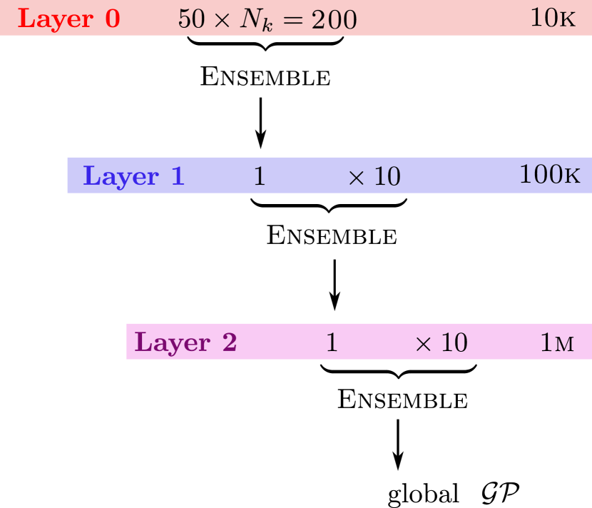
Figure 5: Graphical depiction of the pyramidal structure for ensembles of ensemble GPs.

iv) Solar physics dataset: We used the solar physics dataset (https://solarscience.msfc.nasa.gov/) which consists of $N=3196$ samples. Each input-output data point corresponds to the monthly average estimate of the sunspot counting numbers from 1700 to 1995. The output targets $\bm{y}$ were transformed to the real-valued domain via the mapping $\log(y_{i}+1)$ to use a normal likelihood distribution. We also scaled the input area to the range $\bm{x}\in[0,100]$ and normalized the outputs to be zero-mean. The number of tasks was $K=50$ and $20\%$ of the data observations were reserved for test. The initial values of kernel and likelihood hyperparameters was $\{\ell=0.2,\sigma^{2}_{a}=1.0,\sigma^{2}_{n}=0.1\}$ where $\sigma^{2}_{n}$ is the initial likelihood variance, that we also learn. In this case, the setup of the VEM algorithm was {$\textsc{ve}=20$, $\textsc{vm}=20$, $\eta_{m}=10^{-5}$, $\eta_{L}=10^{-8}$, $\eta_{\psi}=10^{-10}$, $\eta_{Z}=10^{-10}$}. The number of global inducing-inputs used for the ensemble was $M=90$, whilst we used $M_{k}=6$ for each distributed approximation.

v) Pixel-wise MNIST classification: We took images of ones and zeros from the MNIST dataset. To simulate a pixel-wise unsupervised classification problem, true labels of images were ignored. Instead, we threshold the pixels to be greater or smaller than $0.5$, and labeled as $y_{i}=0$ or $y_{i}=1$. That is, we turned the grey-scaled values to a binary coding. Then, all pixels were described by a two-dimensional input in the range $[-1.0,1.0]$, that indicates the coordinate of each output datum. In the case of the zero image, we splitted the data in four areas, i.e. the four corners, as is shown in the subfigure (A) of Figure 4. Each one of the local tasks was initialized with an equally spaced grid of $M_{k}=16$ inducing-inputs. The ensemble GP required $M=25$ in the case of the number zero and $M=16$ for the one. The plotted curves correspond to the test GP predictive posterior at the probit levels $[0.2,0.5,0.8]$. The setup of the VEM algorithm was {$\textsc{ve}=20$, $\textsc{vm}=10$, $\eta_{m}=10^{-3}$, $\eta_{L}=10^{-5}$, $\eta_{\psi}=10^{-6}$, $\eta_{Z}=10^{-5}$}.

vi) Compositional number: As an illustrative experiment of the capabilities shown by the recyclable GP framework, we generated a number eight pixel-wise predictor whitout observing any picture. Instead, we used the $K=4$ distributed tasks of the previous experiment with the number zero. We replicated the objects $\mathcal{E}_{k}$ twice, so the final ensemble input list was $\{\mathcal{E}_{1},\dots,\mathcal{E}_{4},\mathcal{E}_{5},\dots,\mathcal{E}_{8}\}$. The set of partitions $\{\mathcal{E}_{5},\dots,\mathcal{E}_{8}\}$ was identical to the previous ones but we shifted the inducing-inputs $\bm{Z}_{k}$ by adding $1.2$ in the vertical axis. That is, with smaller distributed tasks of two number zeros, we generated an ensemble of a number eight. We remark that this experiment is purely illustrative to show the potential uses of the framework in compositional learning applications. The initial values of hyperparameters and the setup of the optimization algorithm was equivalent to the previous experiment.

vii) Banana dataset: The banana experiment is perhaps one of the most used datasets for testing GP classification models. We followed a similar strategy as the one used in the MNIST experiment. After removing the $33\%$ of samples for testing, we partitioned the input-area in four quadrants, i.e. as is shown in Figure 4. For each partition we set a grid of $M_{k}=9$ inducing-inputs and later, the maximum complexity of the global sparse model was set to $M=25$. The baseline GP classification method also used $M=25$ inducing-inputs and obtained an nlpd value of $7.29\pm 7.85\times 10^{-4}$ after ten trials with different initializations. Our method obtained a test nlpd of $7.21\pm 0.04$. As we mentioned in the main manuscript, the difference is understandable as the recyclable GP framework used a total amount of $4\times 16$ inducing-inputs, that capture more uncertainty than the $16$ of the baseline method. The setup of the VEM algorithm was {$\textsc{ve}=20$, $\textsc{vm}=10$, $\eta_{m}=10^{-3}$, $\eta_{L}=10^{-5}$, $\eta_{\psi}=10^{-6}$, $\eta_{Z}=10^{-5}$}.

viii) London household data: Based on the large scale experiments in Hensman et al. (2013), we obtained the register of properties sold in the Greater London county during the 2017 year (https://www.gov.uk/government/collections/price-paid-data). All addresses of household registers were translated to latitude-longitude coordinates, that we used as the input data points. In our experiment, we selected two heterogeneous registers, one real-valued and the other binary. The real-valued output targets correspond to the log-price of the properties included in the registers. Moreover, the binary values make reference to the type of contract, $y_{i}=1$ if it was a leasehold and $y_{i}=0$ if freehold. Interestingly, we appreciated that both tasks share modes accross the input region, as they are correlated. That is, if there is more presence of some type of contract, it makes sense that the price increases or decreases accordingly. Therefore, after dividing the area of London in the four quadrants $\{Q1,Q2,Q3,Q4\}$ shown in the last Figure of the manuscript, we trained the $Q1$ exclusively with the regression data. Our assumption is that there exists an underlying function $f$ that is linked differently to the parameters depending if the problem is regression or classification. With this in mind, we trained the ensemble bound on the entire area of the city with two local GPs, one coming from regression in $Q1$ and the other from classification in $\{Q2,Q3,Q4\}$. To check if the error results showed an improvement in prediction, we compared the posterior GP prediction of the ensemble GP on $Q1$ with the local GP that did not observe any data on $Q1$. Results showed us, that even after not observing any binary data in $Q1$, the global GP performed better that the local GP with no regression information. The setup of the VEM algorithm was {$\textsc{ve}=20$, $\textsc{vm}=10$, $\eta_{m}=10^{-5}$, $\eta_{L}=10^{-7}$, $\eta_{\psi}=10^{-8}$, $\eta_{Z}=10^{-7}$} and we used $M=25$ inducing-inputs.

Appendix E.2.  Performance metrics

In our experiments, we used three metrics for evaluating the predictive performance of the global GP solutions: i) negative log-predictive density (nlpd), ii) root mean square error (rmse) and iii) mean absolute error (mae). Given a test input datum $\bm{x}_{t}$ and $\{\hat{f}_{t},\hat{y}_{t}\}$ being the predictive mean of the GP function and output prediction respectively, the metrics can be computed as

nlpd $$=-\sum_{t=1}^{N_{t}}\log p(y_{t}|\mathcal{D}),$$

rmse $$=\sqrt{\frac{1}{N_{t}}\sum_{t=1}^{N_{t}}(\hat{f}_{t}-f_{t})^{2}},$$

mae $$=\frac{1}{N_{t}}\sum_{t=1}^{N_{t}}\left|\hat{f}_{t}-f_{t}\right|,$$

where $y_{t}$ and $f_{t}$ are the true output target and function values. $N_{t}$ is the number of test data points.

Appendix E.3.  Optimization algorithms

The following version of the variational expectation-maximization (VEM) algorithm is used both for the local and global inference of GPs. That is the reason why we do not include the sub-scripts $\{k,*\}$ in the parameter variables.

Algorithm 1 — Variational EM for recyclable GPs

1:  Initialize $\bm{\psi},\bm{\phi}$ and $\bm{Z}$

2:  while not $\mathcal{L}^{(t)}_{\mathcal{E}}\approx\mathcal{L}^{(t-1)}_{\mathcal{E}}$ do

3:     # Variational Expectation (VE)

4:     for $j\in 1,\dots,\textsc{ve}$ do

5:        update $\bm{\mu}_{(j)}\leftarrow\bm{\mu}_{(j-1)}+\eta_{\mu}\nabla_{\mu}\mathcal{L}_{\mathcal{E}}$

6:        update $\bm{L}_{(j)}\leftarrow\bm{L}_{(j-1)}+\eta_{L}\nabla_{L}\mathcal{L}_{\mathcal{E}}$

7:     end for

8:     # Variational Maximization (VM)

9:     # Hyperparameters

10:     for $j\in 1,\dots,\textsc{vm}$ do

11:        update $\ell_{(j)}\leftarrow\ell_{(j-1)}+\eta_{\psi}\nabla_{\ell}\mathcal{L}_{\mathcal{E}}$

12:        update $\sigma_{a,(j)}\leftarrow\sigma_{a,(j-1)}+\eta_{\psi}\nabla_{\sigma_{a}}\mathcal{L}_{\mathcal{E}}$

13:     end for

14:     # Inducing-inputs

15:     for $j\in 1,\dots,\textsc{vm}$ do

16:        update $\bm{Z}_{(j)}\leftarrow\bm{Z}_{(j-1)}+\eta_{Z}\nabla_{Z}\mathcal{L}_{\mathcal{E}}$

17:     end for

18:  end while

For the distributed GP regression models needed for the baseline methods, we used the LBFGS optimization algorithm with a learning rate $\eta=10^{-2}$. We set a default maximum of $50$ iterations.

References

- Álvarez and Lawrence (2011) M. A. Álvarez and N. D. Lawrence. Computationally efficient convolved multiple output Gaussian processes. Journal of Machine Learning Research, 12(May):1459–1500, 2011.
- Bordley (1982) R. F. Bordley. A multiplicative formula for aggregating probability assessments. Management Science, 28(10):1137–1148, 1982.
- Bui and Turner (2014) T. D. Bui and R. E. Turner. Tree-structured Gaussian process approximations. In Advances in Neural Information Processing Systems (NIPS), pages 2213–2221, 2014.
- Bui et al. (2017) T. D. Bui, C. Nguyen, and R. E. Turner. Streaming sparse Gaussian process approximations. In Advances in Neural Information Processing Systems (NIPS), pages 3299–3307, 2017.
- Bui et al. (2018) T. D. Bui, C. V. Nguyen, S. Swaroop, and R. E. Turner. Partitioned variational inference: A unified framework encompassing federated and continual learning. arXiv preprint arXiv:1811.11206, 2018.
- Burt et al. (2019) D. R. Burt, C. E. Rasmussen, and M. Van der Wilk. Rates of convergence for sparse variational Gaussian process regression. In International Conference on Machine Learning (ICML), pages 862–871, 2019.
- Cao and Fleet (2014) Y. Cao and D. J. Fleet. Generalized product of experts for automatic and principled fusion of Gaussian process predictions. arXiv preprint arXiv:1410.7827, 2014.
- Deisenroth and Ng (2015) M. Deisenroth and J. W. Ng. Distributed Gaussian processes. In International Conference on Machine Learning (ICML), pages 1481–1490, 2015.
- Gal et al. (2014) Y. Gal, M. Van Der Wilk, and C. E. Rasmussen. Distributed variational inference in sparse Gaussian process regression and latent variable models. In Advances in Neural Information Processing Systems (NIPS), pages 3257–3265, 2014.
- Goodfellow et al. (2014) I. J. Goodfellow, M. Mirza, D. Xiao, A. Courville, and Y. Bengio. An empirical investigation of catastrophic forgetting in gradient-based neural networks. In International Conference on Learning Representations (ICLR), 2014.
- Hensman et al. (2013) J. Hensman, N. Fusi, and N. D. Lawrence. Gaussian processes for big data. In Uncertainty in Artificial Intelligence (UAI), pages 282–290, 2013.
- Hensman et al. (2015) J. Hensman, A. Matthews, and Z. Ghahramani. Scalable variational Gaussian process classification. In Artificial Intelligence and Statistics (AISTATS), pages 351–360, 2015.
- Hinton (2002) G. E. Hinton. Training products of experts by minimizing contrastive divergence. Neural Computation, 14(8):1771–1800, 2002.
- Hoffman et al. (2013) M. D. Hoffman, D. M. Blei, C. Wang, and J. Paisley. Stochastic variational inference. Journal of Machine Learning Research (JMLR), 14(1):1303–1347, 2013.
- Jacobs et al. (1991) R. A. Jacobs, M. I. Jordan, S. J. Nowlan, and G. E. Hinton. Adaptive mixtures of local experts. Neural Computation, 3(1):79–87, 1991.
- Lázaro-Gredilla and Titsias (2011) M. Lázaro-Gredilla and M. K. Titsias. Variational heteroscedastic Gaussian process regression. In International Conference on Machine Learning (ICML), pages 841–848, 2011.
- Matthews et al. (2016) A. G. d. G. Matthews, J. Hensman, R. Turner, and Z. Ghahramani. On sparse variational methods and the Kullback-Leibler divergence between stochastic processes. In Artificial Intelligence and Statistics (AISTATS), pages 231–239, 2016.
- Moreno-Muñoz et al. (2018) P. Moreno-Muñoz, A. Artés-Rodríguez, and M. A. Álvarez. Heterogeneous multi-output Gaussian process prediction. In Advances in Neural Information Processing Systems (NeurIPS), pages 6711–6720, 2018.
- Moreno-Muñoz et al. (2019) P. Moreno-Muñoz, A. Artés-Rodríguez, and M. A. Álvarez. Continual multi-task Gaussian processes. arXiv preprint arXiv:1911.00002, 2019.
- Ng and Deisenroth (2014) J. W. Ng and M. P. Deisenroth. Hierarchical mixture-of-experts model for large-scale Gaussian process regression. arXiv preprint arXiv:1412.3078, 2014.
- Nguyen et al. (2018) C. V. Nguyen, Y. Li, T. D. Bui, and R. E. Turner. Variational continual learning. In International Conference on Learning Representations (ICLR), 2018.
- Peterson et al. (2019) D. Peterson, P. Kanani, and V. J. Marathe. Private federated learning with domain adaptation. Workshop on Federated Learning for Data Privacy and Confidentiality at NeurIPS, 2019.
- Rasmussen and Ghahramani (2002) C. E. Rasmussen and Z. Ghahramani. Infinite mixtures of Gaussian process experts. In Advances in neural information processing systems (NIPS), pages 881–888, 2002.
- Rasmussen and Williams (2006) C. E. Rasmussen and C. K. Williams. Gaussian processes for machine learning, volume 2. MIT Press, 2006.
- Ruiz et al. (2018) F. J. Ruiz, M. K. Titsias, A. B. Dieng, and D. M. Blei. Augment and reduce: Stochastic inference for large categorical distributions. In International Conference on Machine Learning (ICML), 2018.
- Saul et al. (2016) A. D. Saul, J. Hensman, A. Vehtari, and N. D. Lawrence. Chained Gaussian processes. In Artificial Intelligence and Statistics (AISTATS), pages 1431–1440, 2016.
- Seeger (2002) M. Seeger. PAC-Bayesian generalisation error bounds for Gaussian process classification. Journal of Machine Learning Research (JMLR), 3(Oct):233–269, 2002.
- Smith et al. (2017) V. Smith, C.-K. Chiang, M. Sanjabi, and A. S. Talwalkar. Federated multi-task learning. In Advances in Neural Information Processing Systems (NIPS), pages 4424–4434, 2017.
- Titsias (2009) M. Titsias. Variational learning of inducing variables in sparse Gaussian processes. In Artificial Intelligence and Statistics (AISTATS), pages 567–574, 2009.
- Titsias et al. (2020) M. K. Titsias, J. Schwarz, A. G. de G. Matthews, R. Pascanu, and Y. W. Teh. Functional regularisation for continual learning with Gaussian processes. In International Conference on Learning Representations (ICLR), 2020.
- Tresp (2000) V. Tresp. A Bayesian committee machine. Neural Computation, 12(11):2719–2741, 2000.
- Van der Wilk et al. (2017) M. Van der Wilk, C. E. Rasmussen, and J. Hensman. Convolutional Gaussian processes. In Advances in Neural Information Processing Systems (NIPS), pages 2849–2858, 2017.
- Velychko et al. (2018) D. Velychko, B. Knopp, and D. Endres. Making the coupled Gaussian process dynamical model modular and scalable with variational approximations. Entropy, 20(10):724, 2018.