Please Mind the Root: Decoding Arborescences for Dependency Parsing
rz279@cam.ac.uk tim.f.vieira@gmail.com
ryan.cotterell@inf.ethz.ch
Abstract
The connection between dependency trees and spanning trees is exploited by the NLP community to train and to decode graph-based dependency parsers. However, the NLP literature has missed an important difference between the two structures: only one edge may emanate from the root in a dependency tree. We analyzed the output of state-of-the-art parsers on many languages from the Universal Dependency Treebank: although these parsers are often able to learn that trees which violate the constraint should be assigned lower probabilities, their ability to do so unsurprisingly degrades as the size of the training set decreases. In fact, the worst constraint-violation rate we observe is . Prior work has proposed an inefficient algorithm to enforce the constraint, which adds a factor of to the decoding runtime. We adapt an algorithm due to Gabow and Tarjan (1984) to dependency parsing, which satisfies the constraint without compromising the original runtime.111Our Python library is available at https://github.com/rycolab/spanningtrees.
1 Introduction
Developing probabilistic models of dependency trees requires efficient exploration over a set of possible dependency trees, which grows exponentially with the length of the input sentence .
Under an edge-factored model (McDonald et al., 2005; Ma and Hovy, 2017; Dozat and Manning, 2017), finding the maximum-a-posteriori dependency tree is equivalent to finding the maximum weight spanning tree in a weighted directed graph. More precisely, spanning trees in directed graphs are known as arborescences. The maximum-weight arborescence can be found in (Tarjan, 1977; Camerini et al., 1979).222Several authors (e.g., Qi et al. (2020); McDonald et al. (2005)) opt for the simpler CLE algorithm (Chu and Liu, 1965; Bock, 1971; Edmonds, 1967), which has a worst-case bound of , but is often fast in practice.
However, an oversight in the relationship between dependency trees and arborescences has gone largely unnoticed in the dependency parsing literature. Most dependency annotation standards enforce a root constraint: Exactly one edge may emanate from the root node.333A notable exception is the Prague Dependency Treebank Bejček et al. (2013), which allows for multi-rooted trees. For example, the Universal Dependency Treebank (UD; Nivre et al. (2018)), a large-scale multilingual syntactic annotation effort, states in their documentation (UD Contributors, ):
There should be just one node with the root dependency relation in every tree.
This oversight implies that parsers may return malformed dependency trees. Indeed, we examined the output of a state-of-the-art parser (Qi et al., 2020) for UD treebanks. We saw that decoding without a root constraint resulted in (on average) of the decoded dependency trees being malformed. This increased to on languages that contain less than one thousand training instances with the worst case of on Kurmanji.
The NLP literature has proposed two solutions to enforce the root constraint: (1) Allow invalid dependency trees—hoping that the model can learn to assign them low probabilities and decode singly rooted trees, or (2) return the best of runs of the CLE each with a fixed edge emanating from the root (Dozat et al., 2017).444In practice, if constraint violations are infrequent, this strategy should be used as a fallback for when the unconstrained solution fails. However, this will not necessarily be the case, and is rarely the case during model training. The first solution is clearly problematic as it may allow parsers to predict malformed dependency trees. This issue is further swept under the rug with “forgiving” evaluation metrics, such as attachment scores, which give partial credit for malformed output.555We note exact match metrics, which consider the entire arborescence, do penalize root constraint violations The second solution, while correct, adds an unnecessary factor of to the runtime of root-constrained decoding.
In this paper, we identify a much more efficient solution than (2). We do so by unearthing an algorithm due to Gabow and Tarjan (1984) from the theoretical computer science literature. This algorithm appears to have gone unnoticed in NLP literature;666There is one exception: Corro et al. (2016) mention Gabow and Tarjan (1984)’s algorithm in a footnote. we adapt the algorithm to correctly and efficiently handle the root constraint during decoding in edge-factored non-projective dependency parsing.777Much like this paper, efficient root-constrained marginal inference is also possible without picking up an extra factor of , but it requires some attention to detail (Koo et al., 2007; Zmigrod et al., 2020).
[hide label]
{deptext}[column sep=0.1em, row sep=0ex]
& & & & & & & &
root & Someplace & that & is & like & $ & & an & entree &
\depedge[edge height=0.3cm]12
\depedge[edge height=0.9cm]63
\depedge[edge height=0.6cm]64
\depedge[edge height=0.3cm]65
\depedge[edge height=1.2cm]26
\depedge[edge height=0.3cm]67
\depedge[edge height=0.3cm]98
\depedge[edge height=1.5cm, edge style=Crimson, very thick]19
\depedge[edge height=0.6cm, edge style=MediumBlue, very thick, dotted]69
2 Approach
In this section, the marker ![]() indicates that a recently introduced concept is illustrated the worked example in Fig. 2.
Let be a rooted weighted directed graph
where
is a set of nodes,
is a set of weighted edges, ,888When there is no ambiguity, we may abuse notation using to refer to either its node or edge set,
e.g., we may write to mean , and to mean .
and is a designated root node with no incoming edges.
In terms of dependency parsing, each non- node corresponds to a token in the sentence, and represents the special root token that is not a token in the sentence.
Edges represent possible dependency relations between tokens. The edge weights are scores from a model (e.g., linear McDonald et al. (2005), or neural network Dozat et al. (2017)).
Fig. 1 shows an example.
We allow to be a multi-graph, i.e., we allow multiple edges between pairs of nodes.
Multi-graphs are a natural encoding of labeled dependency relations where possible labels between words are captured by multiple edges between nodes in the graph.
Multi-graphs pose no difficulty as only the highest-weight edge between two nodes may be selected in the returned tree.
indicates that a recently introduced concept is illustrated the worked example in Fig. 2.
Let be a rooted weighted directed graph
where
is a set of nodes,
is a set of weighted edges, ,888When there is no ambiguity, we may abuse notation using to refer to either its node or edge set,
e.g., we may write to mean , and to mean .
and is a designated root node with no incoming edges.
In terms of dependency parsing, each non- node corresponds to a token in the sentence, and represents the special root token that is not a token in the sentence.
Edges represent possible dependency relations between tokens. The edge weights are scores from a model (e.g., linear McDonald et al. (2005), or neural network Dozat et al. (2017)).
Fig. 1 shows an example.
We allow to be a multi-graph, i.e., we allow multiple edges between pairs of nodes.
Multi-graphs are a natural encoding of labeled dependency relations where possible labels between words are captured by multiple edges between nodes in the graph.
Multi-graphs pose no difficulty as only the highest-weight edge between two nodes may be selected in the returned tree.
An arborescence of is a subgraph where such that:
-
(C1)
Each non-root node has exactly one incoming edge (thus, );
-
(C2)
has no cycles.
A dependency tree of is an arborescence that additionally satisfies
-
(C3)
In words, (C3) says contains exactly one out-edge from . Let and denote the sets of arborescences and dependency trees, respectively.
The weight of a graph or subgraph is defined as
| (1) |
In § 2.1, we describe an efficient algorithm for finding the best (highest-weight) arborescence
| (2) |
and, in § 2.2, the best dependency tree.999Probabilistic models of arborescences (e.g., Koo et al. (2007); Dozat and Manning (2017)) typically seek the maximum a posteriori structure, . This case can be solved as 1 by taking the weight of to be because .
| (3) |
2.1 Finding the best arborescence
A first stab at finding would be to select the best (non-self-loop) incoming edge for each node. Although, this satisfies (C1), it does not (necessarily) satisfy (C2). We call this subgraph the greedy graph, denoted . Clearly, since it is subject to fewer restrictions. Furthermore, if happens to be acyclic, it is clearly equal to . What are we to do in the event of a cycle? That answer has two parts.
Part 1: We call any cycle in a critical cycle. Naturally, (C2) implies that critical cycles can never be part of an arborescence. However, they help us identify optimal arborescences for certain subproblems. Specifically, if we were to “break” the cycle at any node by removing its (unique) incoming edge, we would have an optimal arborescence rooted at for the subgraph over the nodes in . Let be a subgraph of rooted at that denotes the broken cycle at . Let be the subgraph rooted at where contains all the nodes in and all edges between them from . Since is a critical cycle, is the greedy graph of . Moreover, as it is acyclic, we have that . The key to finding the best arborescence of the entire graph is, thus, determining where to break critical cycles.
Part 2: Breaking cycles is done with a recursive algorithm that solves the “outer problem” of fitting the (unbroken) cycle into an optimal arborescence. The algorithm treats the cycle as a single contracted node. Formally, a cycle contraction takes a graph and a (not necessarily critical) cycle , and creates a new graph denoted with the same root, nodes where is a new node that represents the cycle, and contains the following set of edges: For any
-
•
enter: if , then where . Akin to dynamic programming, this choice edge weight (due to Georgiadis (2003)) gives the best “cost-to-go” for breaking the cycle at .
-
•
exit: if , then
-
•
external: if , then
-
•
dead: if , then no edge related to is in . This is because such an edge would be a self-cycle, which can never be part of an arborescence.
Additionally, we define a bookkeeping function, , which maps the nodes and edges of to their counterparts in . We overload to apply point-wise to the constituent nodes and edges.
By (C1), we have that for any , there exists exactly one incoming edge to the cycle node . We can use to infer where the cycle was broken with . We call the entrance site of . Consequently, we can stitch together an arborescence as . We use the shorthand for this operation due to its visual similarity to unraveling a cycle.
may also have a critical cycle, so we have to apply this reasoning recursively. This is captured by Karp (1971)’s Theorem 1.101010We have lightly modified the original theorem. For completeness, App. A provides a proof in our notation.
Theorem 1.
For any graph , either or contains a critical cycle and where is the entrance site of . Furthermore, .
Theorem 1 suggests a recursive strategy for finding , which is the basis of many efficient algorithms (Tarjan, 1977; Camerini et al., 1979; Georgiadis, 2003; Chu and Liu, 1965; Bock, 1971; Edmonds, 1967). We detail one such algorithm in Alg 1. Alg 1 can be made to run in time for dense with the appropriate implementation choices, such as Union-Find (Hopcroft and Ullman, 1973) to maintain membership of nodes to contracted nodes, as well as radix sort Knuth (1973) to sort incoming edges to contracted nodes; using a regular sort would add a factor of to the runtime.
2.2 Finding the best dependency tree
Gabow and Tarjan (1984) propose an algorithm that does additional recursion at the base case of (the additional if-statement at 5) to recover instead of .
Suppose that the set of edges emanating from the root in is given by and . We consider removing each edge in from . Since may have multiple edges from to , we write to mean deleting all edges with the same edge points as . Let be the graph where is chosen greedily to maximize . Consider the two possible cases:
Optimization case. If has no critical cycles, then must be the best arborescence with one fewer edges emanating from the root than by our greedy choice of .
Reduction case. If has a critical cycle , then all edges in that do not point to are in . If , then is critical cycle in the context of constrained problem and so we can apply Theorem 1 to recover . Otherwise, and we can break at to get , which is comprised of edges in . Therefore, we can find to retrieve . This notion is formalized in the following theorem.111111For completeness, App. B provides a proof of Theorem 2.
Theorem 2.
For any graph with , let be the set of outgoing edges from in . If , then . Otherwise, let for that maximizes , then either or there exists a critical cycle in such that where is the entrance site of .
Theorem 2 suggests a recursive strategy (Alg 1) for finding given . Gabow and Tarjan (1984, Theorem 7.1) prove that such a strategy will execute in and so when combined with (Alg 1) leads to a runtime for finding given a graph . The efficiency of the algorithm amounts to requiring a bound of calls to that will lead to the reduction case in order to obtain any number optimization cases. Each recursive call does a linear amount of work to search for the edge to remove and to stitch together the results of recursion. Rather than computing the greedy graph from scratch, implementations should exploit that each edge removal will only change one element of the greedy graph. Thus, we can find in constant time.
| Setting | # Languages | Malformed rate | Rel. UAS | Rel. Exact Match |
|---|---|---|---|---|
| High | ||||
| Medium | ||||
| Low |
3 Experiment
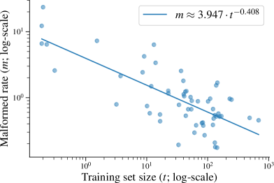
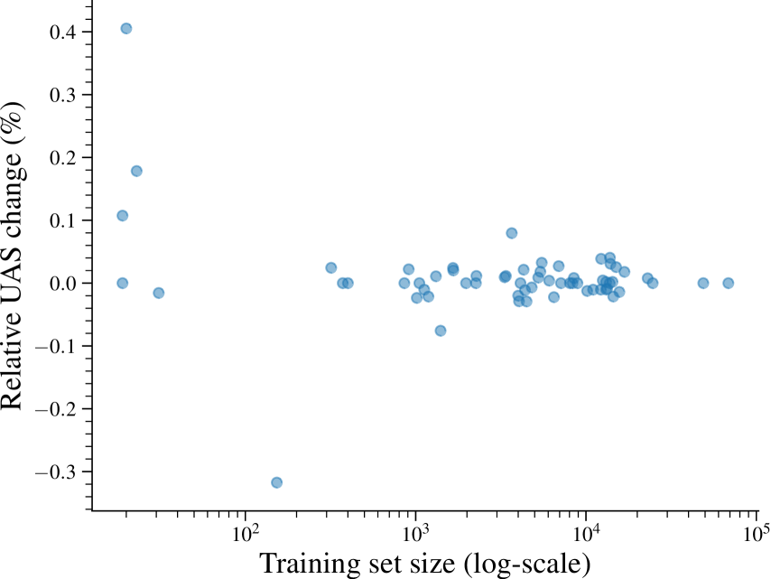
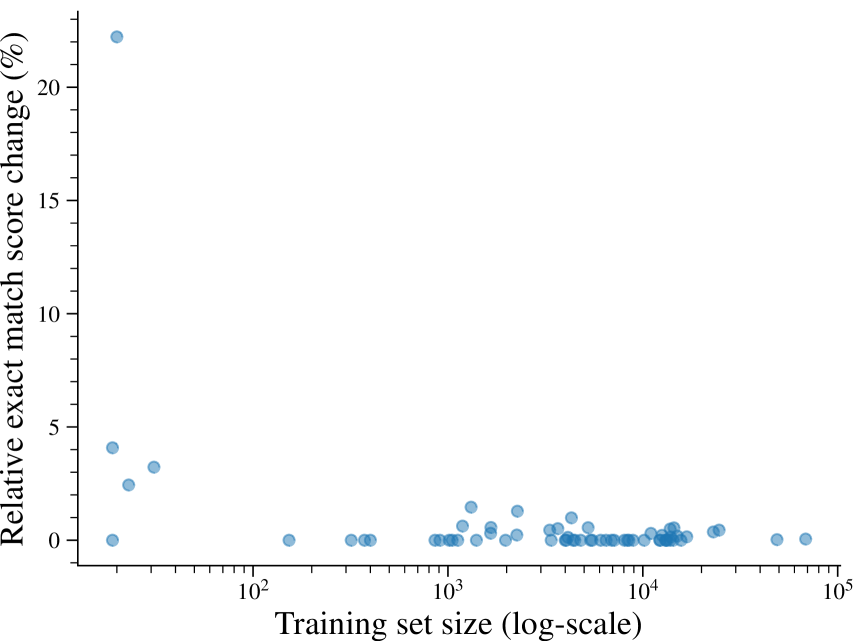
How often do state-of-the-art parsers generate malformed dependency trees? We examined Universal Dependency Treebanks (Nivre et al., 2018) and computed the rate of malformed trees when decoding using edge weights generated by pre-trained models supplied by Qi et al. (2020). On average, we observed that of trees are malformed. We were surprised to see that—although the edge-factored model used is not expressive enough to capture the root constraint exactly—there are useful correlates of the root constraint in the surface form of the sentence, which the model appears to use to workaround this limitation. This becomes further evident when we examine the relative change121212The relative difference is computed with respect to the unconstrained algorithm’s scores. in UAS () and exact match scores () when using the constrained algorithm as opposed to the unconstrained algorithm.
Nevertheless, given less data, it is harder to learn to exploit the surface correlates; thus, we see an increasing average rate of violation, , when examining languages with training set sizes of less than sentences. Similarly, the relative change in UAS and exact match score increases to and respectively. Indeed, the worst violation rate was was seen for Kurmanji which only contains sentences in the training set. Kurmanji consequently had the largest relative changes to both UAS and exact match scores of and . We break down the malformed rate and accuracy changes by training size in Tab. 1. Furthermore, the correlation between training size and malformed tree rate can be seen in Fig. 3 while the correlation between training size and relative accuracy change can be seen in Fig. 4. We provide a full table of the results in App. C.
4 Conclusion
In this paper, we have bridged the gap between the graph-theory and dependency parsing literature. We presented an efficient for finding the maximum arborescence of a graph. Furthermore, we highlighted an important distinction between dependency trees and arborescences, namely that dependency trees are arborescences subject to a root constraint. Previous work uses inefficient algorithms to enforce this constraint. We provide a solution which runs in . Our hope is that this paper will remind future research in dependency parsing to please mind the root.
Acknowledgments
We would like to thank all reviewers for their valuable feedback and suggestions. The first author is supported by the University of Cambridge School of Technology Vice-Chancellor’s Scholarship as well as by the University of Cambridge Department of Computer Science and Technology’s EPSRC.
References
- Bejček et al. (2013) Eduard Bejček, Eva Hajičová, Jan Hajič, Pavlína Jínová, Václava Kettnerová, Veronika Kolářová, Marie Mikulová, Jiří Mírovský, Anna Nedoluzhko, Jarmila Panevová, Lucie Poláková, Magda Ševčíková, Jan Štěpánek, and Šárka Zikánová. 2013. Prague dependency treebank 3.0.
- Bock (1971) F. C. Bock. 1971. An algorithm to construct a minimum directed spanning tree in a directed network. Developments in Operations Research.
- Camerini et al. (1979) Paolo M. Camerini, Luigi Fratta, and Francesco Maffioli. 1979. A note on finding optimum branchings. Networks, 9(4).
- Chu and Liu (1965) Yoeng-Jin Chu and Tseng-Hong Liu. 1965. On the shortest arborescence of a directed graph. Science Sinica, 14.
- Corro et al. (2016) Caio Corro, Joseph Le Roux, Mathieu Lacroix, Antoine Rozenknop, and Roberto Wolfler Calvo. 2016. Dependency parsing with bounded block degree and well-nestedness via Lagrangian relaxation and branch-and-bound. In Proceedings of the 54th Annual Meeting of the Association for Computational Linguistics (Volume 1: Long Papers), pages 355–366, Berlin, Germany. Association for Computational Linguistics.
- Dozat and Manning (2017) Timothy Dozat and Christopher D. Manning. 2017. Deep biaffine attention for neural dependency parsing. In Proceedings of the International Conference on Learning Representations.
- Dozat et al. (2017) Timothy Dozat, Peng Qi, and Christopher D. Manning. 2017. Stanford’s graph-based neural dependency parser at the CoNLL 2017 shared task. In Proceedings of the CoNLL 2017 Shared Task: Multilingual Parsing from Raw Text to Universal Dependencies, Vancouver, Canada. Association for Computational Linguistics.
- Edmonds (1967) Jack Edmonds. 1967. Optimum branchings. Journal of Research of the National Bureau of Standards, Section B: Mathematics and Mathematical Physics, 71(4).
- Gabow and Tarjan (1984) Harold N. Gabow and Robert Endre Tarjan. 1984. Efficient algorithms for a family of matroid intersection problems. Journal of Algorithms, 5(1).
- Georgiadis (2003) Leonidas Georgiadis. 2003. Arborescence optimization problems solvable by Edmonds’ algorithm. Theoretical Computer Science, 301(1-3).
- Hopcroft and Ullman (1973) John E. Hopcroft and Jeffrey D. Ullman. 1973. Set merging algorithms. SIAM J. Comput., 2(4).
- Karp (1971) Richard M. Karp. 1971. A simple derivation of Edmonds’ algorithm for optimum branchings. Networks, 1(3).
- Knuth (1973) Donald E. Knuth. 1973. The Art of Computer Programming, Volume III: Sorting and Searching. Addison-Wesley.
- Koo et al. (2007) Terry Koo, Amir Globerson, Xavier Carreras, and Michael Collins. 2007. Structured prediction models via the matrix-tree theorem. In Proceedings of the Joint Conference on Empirical Methods in Natural Language Processing and Computational Natural Language Learning (EMNLP-CoNLL).
- Ma and Hovy (2017) Xuezhe Ma and Eduard Hovy. 2017. Neural probabilistic model for non-projective MST parsing. In Proceedings of the Eighth International Joint Conference on Natural Language Processing (Volume 1: Long Papers), Taipei, Taiwan. Asian Federation of Natural Language Processing.
- McDonald et al. (2005) Ryan McDonald, Fernando Pereira, Kiril Ribarov, and Jan Hajič. 2005. Non-projective dependency parsing using spanning tree algorithms. In Proceedings of Human Language Technology Conference and Conference on Empirical Methods in Natural Language Processing, Vancouver, British Columbia, Canada. Association for Computational Linguistics.
- Nivre et al. (2018) Joakim Nivre, Mitchell Abrams, Željko Agić, Lars Ahrenberg, Lene Antonsen, Katya Aplonova, Maria Jesus Aranzabe, Gashaw Arutie, Masayuki Asahara, Luma Ateyah, Mohammed Attia, Aitziber Atutxa, Liesbeth Augustinus, Elena Badmaeva, Miguel Ballesteros, Esha Banerjee, Sebastian Bank, Verginica Barbu Mititelu, Victoria Basmov, John Bauer, Sandra Bellato, Kepa Bengoetxea, Yevgeni Berzak, Irshad Ahmad Bhat, Riyaz Ahmad Bhat, Erica Biagetti, Eckhard Bick, Rogier Blokland, Victoria Bobicev, Carl Börstell, Cristina Bosco, Gosse Bouma, Sam Bowman, Adriane Boyd, Aljoscha Burchardt, Marie Candito, Bernard Caron, Gauthier Caron, Gülşen Cebiroğlu Eryiğit, Flavio Massimiliano Cecchini, Giuseppe G. A. Celano, Slavomír Čéplö, Savas Cetin, Fabricio Chalub, Jinho Choi, Yongseok Cho, Jayeol Chun, Silvie Cinková, Aurélie Collomb, Çağrı Çöltekin, Miriam Connor, Marine Courtin, Elizabeth Davidson, Marie-Catherine de Marneffe, Valeria de Paiva, Arantza Diaz de Ilarraza, Carly Dickerson, Peter Dirix, Kaja Dobrovoljc, Timothy Dozat, Kira Droganova, Puneet Dwivedi, Marhaba Eli, Ali Elkahky, Binyam Ephrem, Tomaž Erjavec, Aline Etienne, Richárd Farkas, Hector Fernandez Alcalde, Jennifer Foster, Cláudia Freitas, Katarína Gajdošová, Daniel Galbraith, Marcos Garcia, Moa Gärdenfors, Sebastian Garza, Kim Gerdes, Filip Ginter, Iakes Goenaga, Koldo Gojenola, Memduh Gökırmak, Yoav Goldberg, Xavier Gómez Guinovart, Berta Gonzáles Saavedra, Matias Grioni, Normunds Grūzītis, Bruno Guillaume, Céline Guillot-Barbance, Nizar Habash, Jan Hajič, Jan Hajič jr., Linh Hà Mỹ, Na-Rae Han, Kim Harris, Dag Haug, Barbora Hladká, Jaroslava Hlaváčová, Florinel Hociung, Petter Hohle, Jena Hwang, Radu Ion, Elena Irimia, Ọlájídé Ishola, Tomáš Jelínek, Anders Johannsen, Fredrik Jørgensen, Hüner Kaşıkara, Sylvain Kahane, Hiroshi Kanayama, Jenna Kanerva, Boris Katz, Tolga Kayadelen, Jessica Kenney, Václava Kettnerová, Jesse Kirchner, Kamil Kopacewicz, Natalia Kotsyba, Simon Krek, Sookyoung Kwak, Veronika Laippala, Lorenzo Lambertino, Lucia Lam, Tatiana Lando, Septina Dian Larasati, Alexei Lavrentiev, John Lee, Phuong Lê Hồng, Alessandro Lenci, Saran Lertpradit, Herman Leung, Cheuk Ying Li, Josie Li, Keying Li, KyungTae Lim, Nikola Ljubešić, Olga Loginova, Olga Lyashevskaya, Teresa Lynn, Vivien Macketanz, Aibek Makazhanov, Michael Mandl, Christopher Manning, Ruli Manurung, Cătălina Mărănduc, David Mareček, Katrin Marheinecke, Héctor Martínez Alonso, André Martins, Jan Mašek, Yuji Matsumoto, Ryan McDonald, Gustavo Mendonça, Niko Miekka, Margarita Misirpashayeva, Anna Missilä, Cătălin Mititelu, Yusuke Miyao, Simonetta Montemagni, Amir More, Laura Moreno Romero, Keiko Sophie Mori, Shinsuke Mori, Bjartur Mortensen, Bohdan Moskalevskyi, Kadri Muischnek, Yugo Murawaki, Kaili Müürisep, Pinkey Nainwani, Juan Ignacio Navarro Horñiacek, Anna Nedoluzhko, Gunta Nešpore-Bērzkalne, Luong Nguyễn Thị, Huyền Nguyễn Thị Minh, Vitaly Nikolaev, Rattima Nitisaroj, Hanna Nurmi, Stina Ojala, Adédayọ Olúòkun, Mai Omura, Petya Osenova, Robert Östling, Lilja Øvrelid, Niko Partanen, Elena Pascual, Marco Passarotti, Agnieszka Patejuk, Guilherme Paulino-Passos, Siyao Peng, Cenel-Augusto Perez, Guy Perrier, Slav Petrov, Jussi Piitulainen, Emily Pitler, Barbara Plank, Thierry Poibeau, Martin Popel, Lauma Pretkalniņa, Sophie Prévost, Prokopis Prokopidis, Adam Przepiórkowski, Tiina Puolakainen, Sampo Pyysalo, Andriela Rääbis, Alexandre Rademaker, Loganathan Ramasamy, Taraka Rama, Carlos Ramisch, Vinit Ravishankar, Livy Real, Siva Reddy, Georg Rehm, Michael Rießler, Larissa Rinaldi, Laura Rituma, Luisa Rocha, Mykhailo Romanenko, Rudolf Rosa, Davide Rovati, Valentin Roșca, Olga Rudina, Jack Rueter, Shoval Sadde, Benoît Sagot, Shadi Saleh, Tanja Samardžić, Stephanie Samson, Manuela Sanguinetti, Baiba Saulīte, Yanin Sawanakunanon, Nathan Schneider, Sebastian Schuster, Djamé Seddah, Wolfgang Seeker, Mojgan Seraji, Mo Shen, Atsuko Shimada, Muh Shohibussirri, Dmitry Sichinava, Natalia Silveira, Maria Simi, Radu Simionescu, Katalin Simkó, Mária Šimková, Kiril Simov, Aaron Smith, Isabela Soares-Bastos, Carolyn Spadine, Antonio Stella, Milan Straka, Jana Strnadová, Alane Suhr, Umut Sulubacak, Zsolt Szántó, Dima Taji, Yuta Takahashi, Takaaki Tanaka, Isabelle Tellier, Trond Trosterud, Anna Trukhina, Reut Tsarfaty, Francis Tyers, Sumire Uematsu, Zdeňka Urešová, Larraitz Uria, Hans Uszkoreit, Sowmya Vajjala, Daniel van Niekerk, Gertjan van Noord, Viktor Varga, Eric Villemonte de la Clergerie, Veronika Vincze, Lars Wallin, Jing Xian Wang, Jonathan North Washington, Seyi Williams, Mats Wirén, Tsegay Woldemariam, Tak-sum Wong, Chunxiao Yan, Marat M. Yavrumyan, Zhuoran Yu, Zdeněk Žabokrtský, Amir Zeldes, Daniel Zeman, Manying Zhang, and Hanzhi Zhu. 2018. Universal dependencies 2.3. LINDAT/CLARIN digital library at the Institute of Formal and Applied Linguistics (ÚFAL), Faculty of Mathematics and Physics, Charles University.
- Qi et al. (2020) Peng Qi, Yuhao Zhang, Yuhui Zhang, Jason Bolton, and Christopher D. Manning. 2020. Stanza: A Python natural language processing toolkit for many human languages. In Proceedings of the Association for Computational Linguistics: System Demonstrations.
- Tarjan (1977) Robert Endre Tarjan. 1977. Finding optimum branchings. Networks, 7(1).
- (20) UD Contributors. Root relation in universal dependencies. https://universaldependencies.org/u/dep/root.html. Accessed: 2020-05-30.
- Zmigrod et al. (2020) Ran Zmigrod, Tim Vieira, and Ryan Cotterell. 2020. Efficient computation of expectations under spanning tree distributions. Transactions of the Association for Computational Linguistics.
Appendix A Proof of Theorem 1
To prove Theorem 1, we note a correspondence between graphs and contracted graphs.
Proposition 1.
Given a rooted graph and a (not necessarily critical) cycle in . For any that has a single edge such that and , there exists and such that . Furthermore,
| (4) |
Proof.
Since is the only edge in from a non-cycle node to a cycle node ( enter), every edge such that forms an arborescence . Note that the set of edges in for which there is no corresponding edge in are dead edges. In fact, as satisfies (C1), these edges form an arborescence . Therefore, .
As a corollary, we also have that every arborescence in the contracted graph can be expanded into an arborescence in .
Corollary 1 (Expansion lemma).
Given a rooted graph with a cycle , every arborescence is related to an arborescence by where is the entrance site of . Furthermore .
Proof.
Let be the entrance site of into . As and , Proposition 1 constructs as desired. Furthermore, . ∎
Note that Proposition 1 does not account for all arborescences in . We next show that such arborescences which cannot be constructed using Proposition 1 will never be .
Lemma 1.
Given a rooted graph with a critical cycle . We have that for all
| (10) |
Proof.
Since is a subgraph of it must be that is also a subgraph of . Since is a critical cycle, does not have cycles and equals . Therefore . ∎
Lemma 2.
Given a rooted graph with a critical cycle and . If and such that and , then there exists a with and such that .
Proof.
Construct such that for every edge , if and , then . Additionally, let be in as well as the edges in . Then has no cycles and each non-root node contains a single incoming edge, so . Since and contain identical edges except for those pointing to nodes in , by Lemma 1, . ∎
Theorem 1.
For any graph , either or contains a critical cycle and where is the entrance site of . Furthermore, .
Proof.
There are two cases to consider.
Case 1: does not contain a critical cycle. Trivially, .
Case 2: contains a critical cycle . By Corollary 1, we can construct an arborescence , we now prove that no other can have a higher weight. Firstly, by Lemma 2, we only need to consider that satisfy Proposition 1. Therefore, must be decomposable into an arborescence and an arborescence in where is the entrance site of . Then since is optimal, we have that and . As is optimal (by Lemma 1), must also be optimal and so . ∎
Appendix B Proof of Theorem 2
We prove Theorem 2 by showing that both the optimization and reduction cases described in the main text lead to progress towards finding .
Lemma 3.
For any graph with , let be the set of outgoing edges from in . If , let for that maximizes . If there exists a critical cycle in , then where is the entrance site of .
Proof.
Let and such that . We know that always exists as emanates from the root. By Corollary 1, we know that where is the entrance site of . Furthermore, As has no edges emanating from the root, . There are two cases to consider:
Case 1 (): As is a subgraph of , must have the highest weight in , so .
Case 2 (): Then cannot be in , and the edge pointing to in is the next best possible edge incoming to . Therefore, whichever way we break in , we will get a set of edges with maximal weight and so . ∎
Lemma 4.
For any graph with , let be the set of outgoing edges from in . If , let for that maximizes . Either or there exists a critical cycle in such that where is the entrance site of .
Proof.
Let be the entrance site of . Proof by induction on .
Base case (): If does not contain a critical cycle, then clearly . Since we choose to maximize and is a subgraph of , . Otherwise, has a critical cycle . Then by Lemma 3, .
Inductive case (): Let be the set of outgoing edge from in . Then clearly . If does not contain a critical cycle, then and we satisfy the induction hypothesis. Otherwise, has a critical cycle . Then by Lemma 3, . ∎
Theorem 2.
For any graph with , let be the set of outgoing edges from in . If , then , otherwise if for that maximizes , then either or there exists a critical cycle in such that where is the entrance site of .
Proof.
There are two cases to consider.
Case 1 (): Then has one edge emanating from the root so clearly .
Case 2 (). This is immediate from Lemma 4. ∎
Appendix C Decoding UD Treebanks
| Language | Malformed Rate | Rel. UAS | Rel. Exact Match | ||
|---|---|---|---|---|---|
| Czech | 68495 | 10148 | 0.45% | 0.000% | 0.052% |
| Russian | 48814 | 6491 | 0.49% | 0.000% | 0.027% |
| Estonian | 24633 | 3214 | 0.93% | 0.000% | 0.448% |
| Korean | 23010 | 2287 | 0.96% | 0.008% | 0.366% |
| Latin | 16809 | 2101 | 0.52% | 0.018% | 0.151% |
| Norwegian | 15696 | 1939 | 0.52% | -0.014% | 0.000% |
| Ancient Greek | 15014 | 1047 | 0.57% | 0.026% | 0.186% |
| French | 14450 | 416 | 1.68% | -0.021% | 0.546% |
| Spanish | 14305 | 1721 | 0.17% | 0.002% | 0.000% |
| Old French | 13909 | 1927 | 0.52% | 0.031% | 0.145% |
| German | 13814 | 977 | 1.54% | 0.040% | 0.495% |
| Polish | 13774 | 1727 | 0.00% | 0.000% | 0.000% |
| Hindi | 13304 | 1684 | 0.18% | -0.009% | 0.000% |
| Catalan | 13123 | 1846 | 0.54% | 0.002% | 0.000% |
| Italian | 13121 | 482 | 0.21% | -0.010% | 0.000% |
| English | 12543 | 2077 | 0.48% | 0.004% | 0.217% |
| Dutch | 12264 | 596 | 0.67% | 0.039% | 0.000% |
| Finnish | 12217 | 1555 | 0.39% | -0.010% | 0.000% |
| Classical Chinese | 11004 | 2073 | 0.96% | -0.010% | 0.304% |
| Latvian | 10156 | 1823 | 0.88% | -0.012% | 0.000% |
| Bulgarian | 8907 | 1116 | 0.27% | 0.000% | 0.000% |
| Slovak | 8483 | 1061 | 0.38% | 0.008% | 0.000% |
| Portuguese | 8328 | 477 | 0.42% | 0.000% | 0.000% |
| Romanian | 8043 | 729 | 0.41% | 0.000% | 0.000% |
| Japanese | 7125 | 550 | 0.00% | 0.000% | 0.000% |
| Croatian | 6914 | 1136 | 0.88% | 0.027% | 0.000% |
| Slovenian | 6478 | 788 | 0.38% | -0.022% | 0.000% |
| Arabic | 6075 | 680 | 0.29% | 0.004% | 0.000% |
| Ukrainian | 5496 | 892 | 0.90% | 0.032% | 0.000% |
| Basque | 5396 | 1799 | 0.67% | 0.018% | 0.000% |
| Hebrew | 5241 | 491 | 1.02% | 0.009% | 0.556% |
| Persian | 4798 | 600 | 0.67% | -0.007% | 0.000% |
| Indonesian | 4477 | 557 | 1.26% | -0.029% | 0.000% |
| Danish | 4383 | 565 | 0.53% | -0.011% | 0.000% |
| Swedish | 4303 | 1219 | 1.23% | 0.021% | 0.988% |
| Old Church Slavonic | 4124 | 1141 | 1.05% | 0.000% | 0.128% |
| Urdu | 4043 | 535 | 1.12% | -0.029% | 0.000% |
| Chinese | 3997 | 500 | 1.80% | -0.020% | 0.000% |
| Turkish | 3664 | 983 | 2.54% | 0.080% | 0.513% |
| Gothic | 3387 | 1029 | 0.78% | 0.011% | 0.000% |
| Serbian | 3328 | 520 | 0.19% | 0.009% | 0.446% |
| Galician | 2272 | 861 | 1.16% | 0.011% | 1.282% |
| North Sami | 2257 | 865 | 1.27% | 0.000% | 0.230% |
| Armenian | 1975 | 278 | 0.00% | 0.000% | 0.000% |
| Greek | 1662 | 456 | 0.44% | 0.020% | 0.565% |
| Uyghur | 1656 | 900 | 0.56% | 0.024% | 0.309% |
| Vietnamese | 1400 | 800 | 3.38% | -0.076% | 0.000% |
| Afrikaans | 1315 | 425 | 6.35% | 0.011% | 1.460% |
| Wolof | 1188 | 470 | 1.49% | -0.021% | 0.625% |
| Maltese | 1123 | 518 | 0.58% | -0.010% | 0.000% |
| Telugu | 1051 | 146 | 0.00% | 0.000% | 0.000% |
| Scottish Gaelic | 1015 | 536 | 0.75% | -0.024% | 0.000% |
| Hungarian | 910 | 449 | 4.23% | 0.022% | 0.000% |
| Irish | 858 | 454 | 2.42% | 0.000% | 0.000% |
| Tamil | 400 | 120 | 0.00% | 0.000% | 0.000% |
| Marathi | 373 | 47 | 2.13% | 0.000% | 0.000% |
| Belarusian | 319 | 253 | 0.79% | 0.024% | 0.000% |
| Lithuanian | 153 | 55 | 7.27% | -0.317% | 0.000% |
| Kazakh | 31 | 1047 | 2.58% | -0.016% | 3.226% |
| Upper Sorbian | 23 | 623 | 6.42% | 0.178% | 2.439% |
| Kurmanji | 20 | 734 | 23.57% | 0.405% | 22.222% |
| Buryat | 19 | 908 | 6.61% | 0.107% | 4.082% |
| Livvi | 19 | 106 | 12.26% | 0.000% | 0.000% |