Testing a Data-driven Active Region Evolution Model with Boundary Data at Different Heights from a Solar Magnetic Flux Emergence Simulation

Abstract

A data-driven active region evolution (DARE) model has been developed to study the complex structures and dynamics of solar coronal magnetic fields. The model is configured with typical coronal environment of tenuous gas governed by strong magnetic field, and thus its lower boundary is set at the base of the corona, but driven by magnetic fields observed in the photosphere. A previous assessment of the model using data from a flux emergence simulation (FES) showed that the DARE failed to reproduce the coronal magnetic field in the FES, which is attributed to the fact that the photospheric data in the FES has a very strong Lorentz force and therefore spurious flows are generated in the DARE model. Here we further test the DARE by using three sets of data from the FES sliced at incremental heights, which correspond to the photosphere, the chromosphere and the base of the corona. It is found that the key difference in the three sets of data is the extent of the Lorentz force, which makes the data-driven model perform very differently. At the two higher levels above the photosphere, the Lorentz force decreases substantially, and the DARE model attains results in much better agreement with the FES, confirming that the Lorentz force in the boundary data is a key issue affecting the results of the DARE model. However, unlike the FES data, the photospheric field from SDO/HMI observations has recently been found to be very close to force-free. Therefore, we suggest that it is still reasonable to use the photospheric magnetic field as approximation of the field at the coronal base to drive the DARE model.

1 Introduction

On the solar surface, i.e., the photosphere, magnetic fields are seen to change continuously; magnetic flux emergence brings new flux from the solar interior into the atmosphere, and meanwhile the flux is advected and dispersed by surface motions such as granulation, differential rotation and meridional circulation. Although we are still not able to measure directly the three-dimensional (3D) magnetic field in the atmosphere, in particular, the solar corona, it is believed that the coronal field evolves in response to (or driven by) the changing of the photospheric field. Consequently, complex dynamics occur ubiquitously in the corona, including the interaction of newly emerging field with the pre-existing one, twisting and shearing of the magnetic arcade fields, magnetic reconnection, and magnetic explosions which are manifested as flares and coronal mass ejections.

In macroscopic scale, evolution of the magnetic field in the solar atmosphere is governed by the magnetohydrodynamic (MHD) equations. With magnetic field in the photosphere measured routinely, data-driven models using the photospheric magnetograms as boundary conditions have been proposed in recent years to study the dynamic evolution of solar coronal magnetic field (e.g., Wu et al., 2006; Feng et al., 2012; Cheung & DeRosa, 2012; Jiang et al., 2016; Leake et al., 2017; Inoue et al., 2018; Hayashi et al., 2019; Guo et al., 2019; Pomoell et al., 2019). Due to the limited constraint from observation, data-driven models are developed with very different settings from each other. For simplicity, some used the magneto-frictional model (Cheung & DeRosa, 2012; Pomoell et al., 2019), in which the Lorentz force is balanced by a fictional plasma friction force, and the magnetic field evolves mainly in a quasi-static way. Some used the so-called zero-$\beta$ model (Inoue et al., 2018; Guo et al., 2019), in which the gas pressure and gravity are neglected. It is more realistic to solve the full MHD equations to deal with the nonlinear interaction of the magnetic field with the plasma.

To solve the MHD equations, one needs to specify eight variables (namely plasma density, temperature, and three components of velocity and magnetic field, respectively) in a self-consistent way at the lower boundary as well as in the initial conditions. However, due to the limited observations, they are under-specified. Thus, different choices of initial and boundary conditions have been adopted. For the initial conditions, the background atmosphere was set as a uniformly distributed gas (e.g., Hayashi et al., 2019), an isothermal gas stratified by solar gravity (e.g., Jiang et al., 2016), or a more realistic, highly stratified one with a temperature profile of different levels representing the photosphere, chromosphere and corona (e.g., Jiang et al., 2016a; Guo et al., 2019). The initial settings depend mainly on the interest of study; for instance, if one focuses on the coronal magnetic field, an isothermal gas with typical coronal temperature (e.g., $\sim 10^{6}$ K) and number density (e.g., $\sim 10^{9}$ cm^-3) would be sufficient. However, the choice of typical plasma $\beta$ and Alfvén speed in the calculation is more relevant since in the numerical models it is the dimensionless parameters that matter. So, if one simulates the corona using the full MHD model, the plasma $\beta$ should be typically much less than unity, and the Alfvén speed should be much larger than the sound speed.

Even using the MHD model with typical coronal plasma settings, it is still problematic to specify the lower boundary conditions by using observed data in the photosphere, since the bottom surface in the model is assumed to be the coronal base rather than the photosphere. Certainly, the physical behavior of the photosphere is distinct from that at the coronal height. For example, the key parameter, the plasma $\beta$ in the photosphere is of order unity, and the plasma controls evolution of the magnetic fields. The Alfvén speed in the photosphere is of the order of several km s ^-1, much smaller than the coronal values. Thus, in principle, it is required to use a highly stratified atmosphere model including all the layers from the photosphere to the corona. For example, the simplest form of such stratified atmosphere has been extensively used in MHD simulations of magnetic flux tube emergence from below the photosphere (e.g., Fan, 2001; Archontis et al., 2004; Toriumi & Yokoyama, 2010), which includes a thin isothermal layer representing the photospheric/chromospheric layer (with temperature of about $5000$ K), a narrow transition layer with temperature sharply rising by about two orders of magnitude, and another isothermal layer for the corona. But such settings demand a considerably large amount of computing resources, mainly to resolve the small scale heights in the photosphere and the transition layer, in which the gas density varies by more than eight orders of magnitude within a few megameters. Thus, most of the flux emergence simulations (FESs) currently available only deal with relatively small spatial scales of a few tens of megameters in full three dimensions and short time durations of, typically, hours. The burden of computational resources would be too much if one wants to simulate the long-term (e.g., days) evolution of active-region (AR) size (e.g., hundreds of megameters), which is the main purpose of the data-driven models.

An alternative way to circumvent such technical obstacles is to consider the photospheric data as a reasonable approximation of the corresponding variables at the coronal base. This is what has been done in static extrapolation of coronal magnetic field from the photospheric magnetograms, for instance, the most frequently-used nonlinear force-free field extrapolations from vector magnetograms (e.g., Wiegelmann, 2004; Valori et al., 2007; Wiegelmann & Sakurai, 2012; Jiang & Feng, 2013; Inoue et al., 2014). At relatively large scales, e.g., size of a typical AR, it is generally accepted to approximate the magnetic field at the coronal base by the photospheric field, considering that the large-scale AR field with typical scales of hundreds of megameters do not change much within the thin layer of several megameters from the photosphere, where it is measured, to the coronal base. For instance, Jiang et al. (2016) developed the first full MHD model for data-driven active region evolution (DARE) by using time-sequence of vector magnetograms obtained from SDO/HMI as boundary conditions at the coronal base. They managed to simulate the coronal magnetic field evolution in a flux-emerging AR leading to an eruption and attained a reasonable agreement with SDO/AIA observations. Further applications of this DARE model, e.g., in Jiang et al. (2016b) and He et al. (2020), reveals the formation and reconnection of current sheet and magnetic flux rope involved in major solar flares. See Toriumi & Wang (2019) for further review on DARE models of flare-productive active regions.

Nevertheless, such approximation of magnetic field at the coronal base by the photospheric field should be taken with cautions. For instance, smoothing is required because magnetic structures are broadened from the photosphere to the corona due to the expansion of the fields. Yamamoto & Kusano (2012) showed that the field measured at the chromosphere is best correlated with the simultaneously observed photospheric field that is smoothed by a Gaussian window of about 2 arcsecs (see also Kawabata et al., 2020). A more critical issue is the Lorentz force contained in the photospheric field. Since the plasma $\beta$ is large, it is thought that the photospheric field has a strong Lorentz force to balance the gas pressure gradients. For instance, in classical models of solar magnetic flux emergence, the toroidal flux generated in the tachocline can rise through the convection zone with the aid of magnetic buoyancy force. However, at the photosphere, it is trapped because of the strongly sub-adiabatic stratification there, and its subsequent rising into the atmosphere must resort to the Parker instability (Parker, 1955; Shibata et al., 1989; Archontis et al., 2004), which is a kind of magnetic Rayleigh-Taylor instability. To trigger the Parker instability, the magnetic flux piles up shallowly below the photosphere, until the Lorentz force is built up as large as the gas pressure gradient to hold up an extra amount of mass against gravity, and further ascent of the magnetic flux depends mainly on liberation of the gravity potential energy of this extra amount of mass (Newcomb, 1961; Acheson, 1979; Archontis et al., 2004). This process has been termed “two-step emergence” (e.g., Toriumi & Yokoyama, 2010), and it naturally results in a strongly non-force-free photosphere, which has been indeed shown in typical numerical simulations of idealized flux tube emergence from below the photosphere into the corona.

Thus, if the photospheric magnetic field is introduced in the data-driven MHD model that uses typical settings of atmosphere in the corona, such a strong Lorentz force cannot be balanced by the tenuous plasma. It can induce largely spurious plasma motions, which in turn amplify the magnetic field by the magnetic induction equation, and could make the evolution runaway. This is indeed observed in a recent joint comparative study of 4 different data-driven models (Cheung & DeRosa, 2012; Jiang et al., 2016; Guo et al., 2019; Hayashi et al., 2019) using the photospheric magnetograms produced in a FES as input to their bottom boundaries (Toriumi et al., 2020). It was found in Toriumi et al. (2020) that, although all data-driven models successfully reproduced a flux rope structure, the quantitative discrepancies are very large, and this is attributed mainly to the highly non-force-free input photospheric field and to the different settings of the background atmosphere in the models. Especially, the simulated magnetic flux rope in Jiang et al. (2016)’s DARE model, which uses typical settings of tenuous atmosphere in the corona (i.e., low plasma $\beta$ and high Alfvén speed), exhibits a significantly larger size and stronger magnetic twist than those in the FES as well as the other data-driven MHD models that use much denser plasma at the lower boundary (e.g., Hayashi et al., 2019; Guo et al., 2019). Moreover, the magnetic energy and helicity produced by the DARE model are approximately ten times larger than their original values in the FES. By checking the simulation data near the lower boundary, Toriumi et al. (2020) showed clearly such a big discrepancy arises from the fact that the strong Lorentz force (and torque) in the photospheric field in the FES, originally balanced by the photospheric plasma gravity and pressure, exerts directly on the tenuous plasma in the DARE model. As a result, the plasma is pushed upward and rotated strongly there, making the magnetic field expands quickly and twisted freely, which finally leads to an over-amplification of magnetic energy and helicity in the corona.

However, such a strong runaway expansion of the coronal field as well as its unreasonable level of energy and helicity are not seen in DARE simulations by using the observed magnetograms as the driving boundary conditions (e.g., Jiang et al., 2016, 2016b; He et al., 2020). That is, the result of DARE simulation driven by the FES output data behaves quite distinctly from that driven by actual observational data; the former shows an unreasonable runaway expansion while the latter does not. As mentioned before, the runaway expansion results from strong Lorentz force and torque resident in the boundary data from the FES. This led us to a hypothesis that the actual photospheric field is close to force free, unlike the simulated one in the flux emergence model. Very recently, Duan et al. (2020) statistically surveyed how large Lorentz force is contained in the photospheric magnetic fields observed by SDO/HMI. They computed the normalized Lorentz forces and torques for emerging ARs using a substantially large sample of vector magnetograms (a total number of 3536 set of vector magnetograms from 51 ARs covering the time from 2010 to 2019), and concluded that the photospheric field is very close to a force-free state, since they have a rather small Lorentz force and torque on average with normalized values of $\sim 0.1$, which is clearly not consistent with theories as well as idealized simulations of flux emergence. Furthermore, such a result appears to be not influenced by the sizes of emerging ARs, the emergence rate, or the non-potentiality of the emerging field.

As mentioned before, if a highly forced bottom boundary data is introduced to the DARE model, it fails to reproduce the coronal magnetic field. On the other hand, the observed photospheric field is actually close to force-free. So, the purpose of this paper is to confirm that with a more force-free boundary field, the DARE model can reproduce the coronal magnetic field that is in better agreement with the FES. Although the magnetic field in the photospheric level in the FES is far from force-free, it relaxes quickly to an approximately force-free state when the field emerges into the atmosphere by a few scale heights above the photosphere, because of the fast decreasing of the plasma density and pressure with height (Fan, 2009). Thus, to obtain such a more force-free boundary field from the FES model, we use the data sliced at two more heights above $z=0$ (corresponding to the height of photosphere in the FES model), which is used to mimic the data at the chromosphere and coronal base.

The paper is organized as follows. In Section 2, we give a brief description of the FES and DARE models, and the Lorentz force and torque in the data sets from FES that are used to drive the DARE model. The results of using different boundary data for the DARE are compared in Section 3. Then we conclude in Section 4.

Figure 1: Magnetic flux (top), normalized Lorentz force (middle) and torque (bottom) in the FES data. From left to right are results for the Z00, Z10, and Z20 slices, respectively

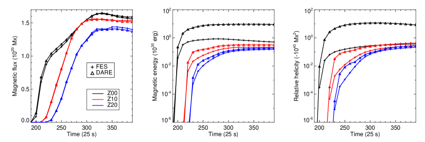
Figure 2: Comparison of magnetic flux, energy and relative helicity in the three DARE tests with their original values.

2 Flux Emergence Simulation and Data-driven MHD Model

Same as Toriumi et al. (2020), we use the boundary data sliced from the FES carried out by Toriumi & Takasao (2017). The numerical code is based on Takasao et al. (2015), and it solves the MHD process of an isolated, twisted magnetic flux tube, initially placed in the convection zone, buoyantly rising into the atmosphere. The full set of basic resistive, adiabatic MHD equations in conservative form are solved by a finite difference scheme with the spatial derivatives by the fourth-order central differences and the temporal derivatives by the four-step Runge-Kutta scheme. Periodic boundary conditions are applied for the $x$-direction and symmetric boundaries for both the $y$- and $z$-directions. The initial background atmosphere of the simulation is gravitationally stratified, which consists of an adiabatically temperature-gradient convection zone ($z/H_{0}<0$, where $H_{0}=170$ km is the length unit of the FES model), the cool isothermal photosphere/chromosphere ($0\leq z/H_{0}<18$), and the hot isothermal corona ($z/H_{0}\geq 18$). The flux tube is initially placed at $z=-30H_{0}$ with the form of $B_{x}(r)=B_{\rm tube}\exp(-r^{2}/R_{\rm tube})$ and $B_{\phi}(r)=qrB_{x}(r)$, where $r$ is the radial distance from the tube’s axis, $R_{\rm tube}=3H_{0}$ the radius, $B_{\rm tube}=7.5$ kG the axial field strength, and $q=-0.2/H_{0}$ the twist intensity (the negative sign indicates a left-handed twist). The middle of the tube is made buoyant by a small density deficiency and the tube started to emerge due to its own buoyancy.

As the time-dependent bottom boundary data for data-driven model, we extracted the time sequence of 2D data at fixed heights from the FES model. To test the behavior of the data-driven model with different inputs, data sets at three different slices from the FES model are used, including $z/H_{0}=0$ (referred to Z00, representing the photosphere), $z/H_{0}=10$ (Z10, i.e., the chromospheric layer) and $z/H_{0}=20$ (Z20, i.e., the coronal base). The slices were sampled at every $\Delta t/\tau_{0}=1$ (where $\tau_{0}=25$ s is the time unit of the FES model) from $t/\tau_{0}=$ 0 to 500. The slices spanned over $(-165,-165)\leq(x/H_{0},y/H_{0})\leq(165,165)$, resolved by the uniform grid spacing of $200\times 200$, thus the resolution is $\Delta=1.65H_{0}$. The data sets include three components of magnetic and velocity field, i.e., $B_{x},B_{y},B_{z},v_{x},v_{y}$, and $v_{z}$.

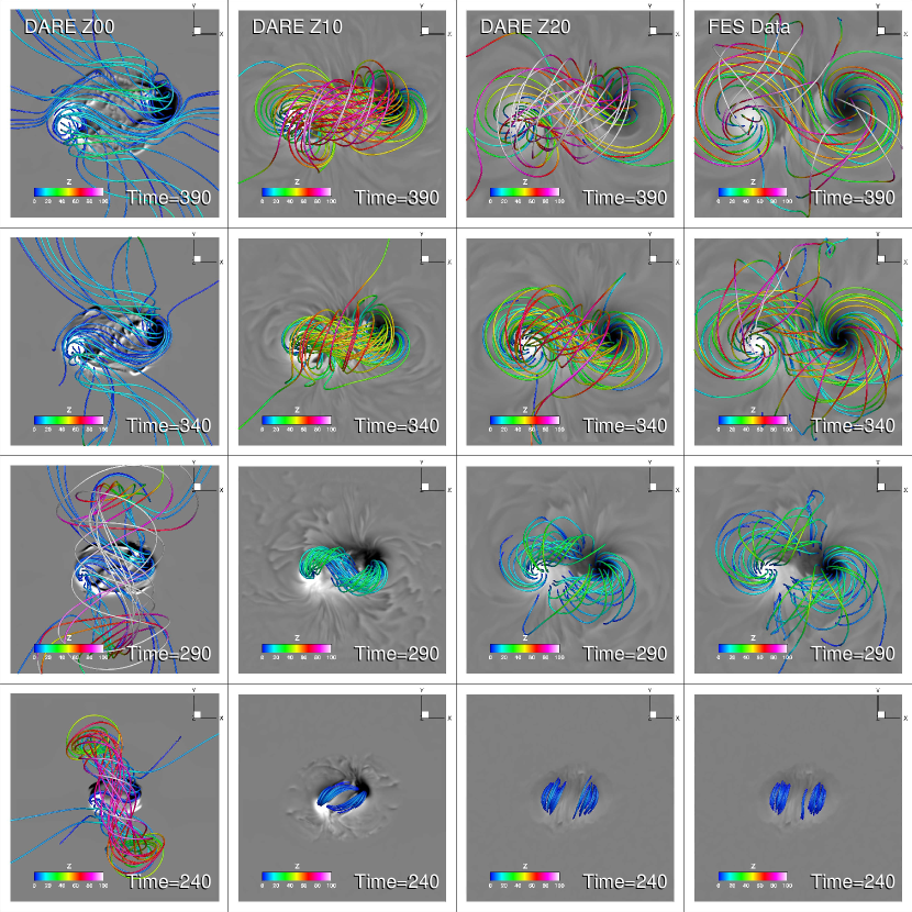
Figure 3: Comparison of magnetic field lines at four time snapshots in the three DARE tests with the original FES data. Note that since different models have different bottom boundaries, the footpoints of the magnetic field lines are not generally idential, but they are all located within the main polarities. Colors of the field lines denote the height above the bottom surface.

As we have mentioned in Section 1, the Lorentz force in the boundary data is an important factor affecting the output of the data-driven model. Thus we quantitatively assess the Lorentz force as well as torque in the data of different layers. The sum of Lorentz force ${\mathbf{F}}$ (and torque ${\mathbf{T}}$) in a volume can be expressed by surface integral (Aly, 1989; Sakurai, 1989), and by neglecting contribution from the side and top boundaries, they can be written as integrals of the 2D data sets:

$$\begin{split}F_{x}=-\frac{1}{4\pi}\int B_{x}B_{z}dxdy,\\ F_{y}=-\frac{1}{4\pi}\int B_{y}B_{z}dxdy,\\ F_{z}=-\frac{1}{8\pi}\int(B_{z}^{2}-B_{x}^{2}-B_{y}^{2})dxdy,\end{split}$$ (1)

and

$$\begin{split}T_{x}=-\frac{1}{8\pi}\int y(B_{z}^{2}-B_{x}^{2}-B_{y}^{2})dxdy,\\ T_{y}=\frac{1}{8\pi}\int x(B_{z}^{2}-B_{x}^{2}-B_{y}^{2})dxdy,\\ T_{z}=\frac{1}{4\pi}\int(yB_{x}B_{z}-xB_{y}B_{z})dxdy.\end{split}$$ (2)

Following Duan et al. (2020), to assess the data with respect to the force-free condition, the forces can be normalized by the integrated magnetic pressure force $F_{p}$ that is given by

$$F_{p}=\left|\int\left(-\nabla\frac{B^{2}}{8\pi}\right)dV\right|=\frac{1}{8\pi}\int(B_{x}^{2}+B_{y}^{2}+B_{z}^{2})dxdy,$$ (3)

and the normalized forces are ratios defined as $f_{x}=|{F_{x}}|/{F_{p}}$, $f_{y}=|{F_{y}}|/{F_{p}}$, and $f_{z}=|{F_{z}}|/{F_{p}}$, respectively. Similarly, the normalized torques are defined as $t_{x}=|{T_{x}}|/{T_{p}}$, $t_{y}=|{T_{y}}|/{T_{p}}$, and $t_{z}=|{T_{z}}|/{T_{p}}$, where $T_{p}$ is magnitude of the net torque induced by only the magnetic pressure force, $T_{p}=|\int{\mathbf{r}}\times(-\nabla\frac{B^{2}}{8\pi})dV|=\sqrt{T_{px}^{2}+T_{py}^{2}}$ where

$$\begin{split}T_{px}=\frac{1}{8\pi}\int y(B_{x}^{2}+B_{y}^{2}+B_{z}^{2})dxdy,\\ T_{py}=\frac{1}{8\pi}\int x(B_{x}^{2}+B_{y}^{2}+B_{z}^{2})dxdy.\end{split}$$ (4)

For a field being close to force-free, it must have all the ratios much less than unity, i.e., $(f_{x},f_{y},f_{z})\ll 1$ and $(t_{x},t_{y},t_{z})\ll 1$. Metcalf et al. (1995) suggested that the magnetic field can be considered as force-free if the normalized forces are all less than or equal to $0.1$, and this criterion is widely accepted by the later studies (Moon et al., 2002; Tiwari, 2012; Liu et al., 2013; Liu & Hao, 2015; Jiang & Zhang, 2019; Duan et al., 2020). On the other hand, for a strongly non force-free field, the ratios can be close to unity, meaning that the magnetic pressure force and the tension force are so unbalanced that the net Lorentz force is comparable to one of its components, the total magnetic pressure force.

In Figure 1, we show these metrics of the FES data. As can be seen, the FES data at the photosphere (i.e., Z00 slice) has a very large verical Lorentz force and horizontal torque, since $f_{z}$, $t_{x}$ and $t_{y}$ are close to $1$ for the whole duration of evolution with the flux injection to its saturation. Note that it is due to the perfect symmetry of two emerging polarities in the simulations that the net forces in horizontal directions (i.e., $f_{x}$ and $f_{y}$) and the net torques in vertical direction ($t_{z}$) are both nearly zero. For comparison, Duan et al. (2020) showed that these parameters derived from SDO/HMI data of emerging ARs are close to $0.1$, which is much smaller than those of the simulated data . At the two higher levels (i.e., Z10 and Z20), the Lorentz force and torque in the early phase of emergence are still large, but decrease substantially with the increase of the magnetic flux, indicating that at these levels the fields are relaxing to a more force-free state. But it should be noted that they are still larger than typical observed values (see also Duan et al., 2020).

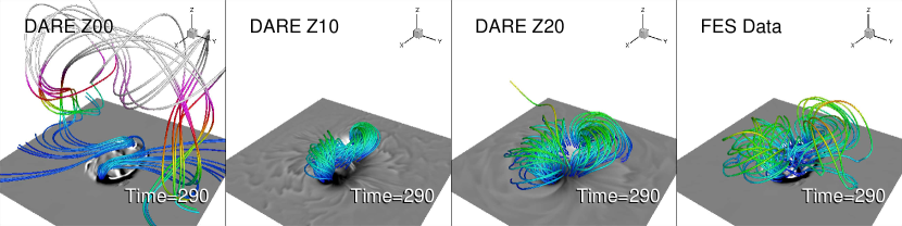
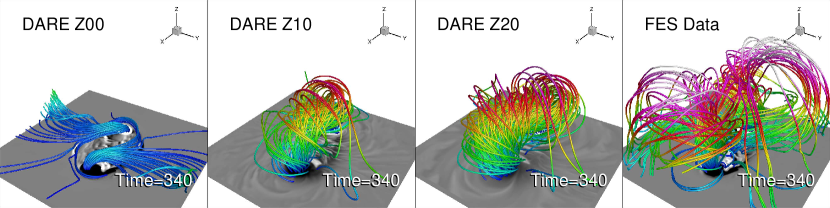
Figure 4: Comparison of magnetic field lines at $t=290$ and $t=340$ in a 3D view.

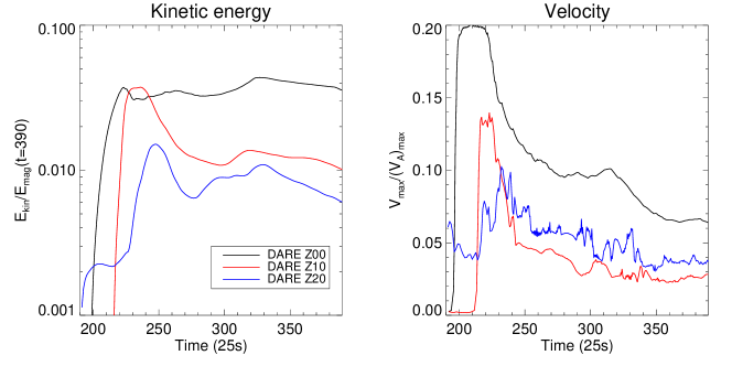
Figure 5: Comparison of kinetic energy and maximal velocity in the three tests.

Jiang et al. (2016)’s data-driven active-region evolution (DARE) model is aimed for reproducing the coronal magnetic field evolution by assuming the bottom surface as the base of the corona. Like the FES model, it solves the full set of the MHD equations with both gas pressure and solar gravity. Also the adiabatic energy equation is used. The numerical code that solves the MHD equations is developed based on the space-time conservative element and solution element (CESE) scheme (Jiang et al., 2010) with a second-order accuracy, and in this code, all MHD variables are specified at the corners of the grid cells and no ghost cells (or guard cells) are used at the boundaries. Since the data-driven simulation is started before the field emerges into the photosphere, the initial conditions consist of a zero magnetic field and a plasma in hydrostatic equilibrium. In all experiments, we used the same initial background atmosphere: plasma stratified by the solar gravity with a uniform temperature of typical coronal value ($T=10^{6}$ K). The bottom boundary of the model is placed at the coronal base with a fixed number density of $10^{9}$ cm^-3 (also a typical value in the corona). After non-dimensionalization, the plasma density and gas pressure at the bottom boundary are both $1$. For all experiments, we used the same computational grid, which has an extent of $(-192,-192,0)\leq(x/\Delta,y/\Delta,z/\Delta)\leq(192,192,384)$ with grid resolution of $\Delta$, where $\Delta=1.65H_{0}$ is the resolution of the input FES data slice. Note that the computational box is nearly twice the size of the FES magnetogram, thus it can effectively reduce the influence from the side and top boundaries (where the plasma variables are all fixed, the horizontal magnetic field is linearly extrapolated and the normal magnetic field is modified to fulfill the divergence-free constraint). On the bottom boundary, the temporally-evolving magnetic field and velocity at a given slice from the FES model are introduced sequentially while the plasma density and temperature are fixed. The boundary data of the FES model is provided at a fixed time cadence of 25 s. However, because the time step of the DARE model is variable according to the CFL stable condition, we use a linear interpolation (in the time domain) at each DARE time step to obtain the boundary data at the exact moment. The magnetic field and velocity outside the field-of-view of the input FES slice are assumed to be zero. For saving computing time, we run all the data-driven simulation with time from $t/\tau_{0}=190$ to $390$, since before $t/\tau_{0}=190$ the magnetic flux has not yet reached the photosphere $z/H_{0}=0$.

3 Results

We test the behavior of the DARE model by driving it with different slices of FES data. Since the magnetic field strength of different slices are different, and to make the comparison within the very same conditions, the magnetic field of each slice are scaled such that the maximum of $B_{z}$ at the bottom boundary is $10$ (non-dimensionalized) in the whole evolution. Thus the maximum Alfvén speed is approximately $10$ (normalized by the sound speed), and smallest plasma $\beta$ is $0.02$, representing a typical low-$\beta$ environment in the corona.

We compare the DARE results with the original FES 3D data in exactly the same volume of $(-100,-100,z_{\rm FES})\leq(x/\Delta,y/\Delta,z/\Delta)\leq(100,100,z_{\rm FES}+200)$ where $z_{\rm FES}=$ Z00, Z10, and Z20, respectively, and the same resolution of $dx=dy=dz=\Delta$. Two global quantities of the magnetic field are calculated, which are the magnetic energy and relative magnetic helicity. Here the relative helicity is obtained by using the method of Valori et al. (2012). Figure 2 shows the results of magnetic energy and helicity. It can be seen that the DARE-Z00 results are larger than that of the FES by an order of magnitude in both magnetic energy and helicity, in agreement with the results shown by Toriumi et al. (2020). The DARE-Z10 and DARE-Z20 results appear to be increasingly better, in particular, the DARE-Z20 produces both energy and helicity matching their original values very closely.

Figures 3 and 4 present the magnetic field lines. The DARE-Z00 shows a drastic expansion at the very early phase like the previous result shown by Toriumi et al. (2020), which makes the magnetic field lines mostly extend out of the box after around $t=300$. Such a drastic expansion is not seen in the results of DARE-Z10 and Z20, both of which consist of a relatively coherent flux rope at $t=340$. As can be seen from the field lines, the DARE results are getting better agreement with the FES with the increasing geometrical level of input data.

Finally, Figure 5 shows the evolutions of the ratio of the kinetic energy (and the largest velocity) to the magnetic energy (and the largest Alfvén speed) in the three experiments. For DARE-Z00, the kinetic energy keeps at the level of 4% of the total magnetic energy over the whole computational duration. This is because the large Lorentz force at the boundary continuously drives the plasma flow. For DARE-Z10, the kinetic energy first rises to the same value as in DARE-Z00, but drops very quickly to roughly 1% of magnetic energy, as the Lorentz force at the bottom boundary deceases. As the Z20 data is even closer to force-free, the kinetic energy is smaller. The similar conclusions can be seen from the ratio of the flow speed to the Alfvén speed. For instance, the Z00 data drives a velocity reaching $0.2$ of the largest Alfvén speed, indicating that the strong Lorentz force results in a very dynamic flow. For the other two experiments, the velocity is smaller than the Alfvén speed by approximately two orders of magnitude, suggesting that the MHD system evolves in a quasi-static way.

4 Conclusions

Toriumi et al. (2020) have investigated different types of data-driven coronal field models using an FES as a reference or ground truth data set. It is found that in the FES the photospheric magnetic field contains a strong Lorentz force, which was too large for the DARE model to reasonably reproduce the coronal magnetic field because unphysical, spurious flows are excited.

In this paper, we have comprehensively compared the DARE simulations driven by three different levels of data from the FES, corresponding to the photosphere (Z00), the chromosphere (Z10) and the base of corona (Z20). The key difference of the three sets of data is the extents of the Lorentz force. In the Z00 data, the field is far from a force-free state with a normalized Lorentz force and torque approaching unity. In the Z10 and Z20, the normalized force and torque decrease substantially. As a result, the DARE model attains much better results of the coronal magnetic field by using the Z10 and Z20 data than using the Z00 data. In particular, by using the Z20 data, which has the smallest Lorentz force among all, the DARE model reproduced the magnetic energy and helicity in a high confidence. Thus, in this experiment, we have confirmed that the Lorentz force in the boundary data is a key issue influences the results of the DARE model. It would be better to use observations for the chromosphere, or even higher in the coronal base as the driving boundary data for the DARE model since the field at the higher levels would be more force-free. Nevertheless, as the recent statistical study by Duan et al. (2020) reveals, the photospheric field of dynamically emerging flux is in fact close to the force-free state unlike the FES model (in particular in Z00). Therefore, it is still possible to use the observed photospheric field as an approximate of coronal base field for driving the data-driven models, such as the DARE. Future investigations using realistic convective FES models that yield more relaxed emergence (e.g., Toriumi & Hotta, 2019; Hotta & Iijima, 2020) may allow us to understand how accurate the data-driven models actually are.

References

- Acheson (1979) Acheson, D. J. 1979, Solar Physics, 62, 23, doi: 10.1007/BF00150129
- Aly (1989) Aly, J. J. 1989, Sol. Phys., 120, 19, doi: 10.1007/BF00148533
- Archontis et al. (2004) Archontis, V., Moreno-Insertis, F., Galsgaard, K., Hood, A., & O’Shea, E. 2004, Astronomy & Astrophysics, 426, 1047, doi: 10.1051/0004-6361:20035934
- Cheung & DeRosa (2012) Cheung, M. C. M., & DeRosa, M. L. 2012, The Astrophysical Journal, 757, 147, doi: 10.1088/0004-637X/757/2/147
- Duan et al. (2020) Duan, A., Jiang, C., Toriumi, S., & Syntelis, P. 2020, arXiv:2005.10532 [astro-ph, physics:physics]. http://arxiv.org/abs/2005.10532
- Fan (2001) Fan, Y. 2001, ApJ, 554, L111, doi: 10.1086/320935
- Fan (2009) —. 2009, ApJ, 697, 1529, doi: 10.1088/0004-637X/697/2/1529
- Feng et al. (2012) Feng, X., Jiang, C., Xiang, C., Zhao, X., & Wu, S. T. 2012, The Astrophysical Journal, 758, 62, doi: 10.1088/0004-637X/758/1/62
- Guo et al. (2019) Guo, Y., Xia, C., Keppens, R., Ding, M. D., & Chen, P. F. 2019, The Astrophysical Journal, 870, L21, doi: 10.3847/2041-8213/aafabf
- Hayashi et al. (2019) Hayashi, K., Feng, X., Xiong, M., & Jiang, C. 2019, The Astrophysical Journal, 871, L28, doi: 10.3847/2041-8213/aaffcf
- He et al. (2020) He, W., Jiang, C., Zou, P., et al. 2020, The Astrophysical Journal, 892, 9, doi: 10.3847/1538-4357/ab75ab
- Hotta & Iijima (2020) Hotta, H., & Iijima, H. 2020, Monthly Notices of the Royal Astronomical Society, 494, 2523, doi: 10.1093/mnras/staa844
- Inoue et al. (2014) Inoue, S., Hayashi, K., Magara, T., Choe, G. S., & Park, Y. D. 2014, The Astrophysical Journal, 788, 182. http://stacks.iop.org/0004-637X/788/i=2/a=182
- Inoue et al. (2018) Inoue, S., Kusano, K., Büchner, J., & Skála, J. 2018, Nature communications, 9, 174
- Jiang & Feng (2013) Jiang, C., & Feng, X. 2013, ApJ, 769, 144, doi: 10.1088/0004-637X/769/2/144
- Jiang et al. (2016a) Jiang, C., Wu, S. T., & Feng, X. 2016a, Frontiers in Astronomy and Space Sciences, 3, 16
- Jiang et al. (2016b) Jiang, C., Wu, S. T., Yurchyshyn, V. B., et al. 2016b, ApJ, 828, 62
- Jiang & Zhang (2019) Jiang, C.-q., & Zhang, M. 2019, Chinese Astronomy and Astrophysics, 43, 252, doi: 10.1016/j.chinastron.2019.04.009
- Jiang et al. (2010) Jiang, C. W., Feng, X. S., Zhang, J., & Zhong, D. K. 2010, Sol. Phys., 267, 463
- Jiang et al. (2016) Jiang, C. W., Wu, S. T., Feng, X. S., & Hu, Q. 2016, Nature Comm., 7, 11522, doi: 10.1038/ncomms11522
- Kawabata et al. (2020) Kawabata, Y., Asensio Ramos, A., Inoue, S., & Shimizu, T. 2020, ApJ, 898, 32, doi: 10.3847/1538-4357/ab9816
- Leake et al. (2017) Leake, J. E., Linton, M. G., & Schuck, P. W. 2017, The Astrophysical Journal, 838, 113, doi: 10.3847/1538-4357/aa6578
- Liu & Hao (2015) Liu, S., & Hao, J. 2015, Advances in Space Research, 55, 1563, doi: 10.1016/j.asr.2015.01.010
- Liu et al. (2013) Liu, S., Su, J. T., Zhang, H. Q., et al. 2013, Publications of the Astronomical Society of Australia, 30, e005, doi: 10.1017/pasa.2012.005
- Metcalf et al. (1995) Metcalf, T. R., Jiao, L., McClymont, A. N., Canfield, R. C., & Uitenbroek, H. 1995, ApJ, 439, 474, doi: 10.1086/175188
- Moon et al. (2002) Moon, Y.-J., Choe, G. S., Yun, H. S., Park, Y. D., & Mickey, D. L. 2002, The Astrophysical Journal, 568, 422, doi: 10.1086/338891
- Newcomb (1961) Newcomb, W. A. 1961, Physics of Fluids, 4, 391, doi: 10.1063/1.1706342
- Parker (1955) Parker, E. N. 1955, The Astrophysical Journal, 122, 293, doi: 10.1086/146087
- Pomoell et al. (2019) Pomoell, J., Lumme, E., & Kilpua, E. 2019, Solar Physics, 294, 41, doi: 10.1007/s11207-019-1430-x
- Sakurai (1989) Sakurai, T. 1989, Space Sci. Rev., 51, 11, doi: 10.1007/BF00226267
- Shibata et al. (1989) Shibata, K., Tajima, T., Matsumoto, R., et al. 1989, The Astrophysical Journal, 338, 471, doi: 10.1086/167212
- Takasao et al. (2015) Takasao, S., Fan, Y., Cheung, M. C. M., & Shibata, K. 2015, ApJ, 813, 112, doi: 10.1088/0004-637X/813/2/112
- Tiwari (2012) Tiwari, S. K. 2012, The Astrophysical Journal, 744, 65, doi: 10.1088/0004-637X/744/1/65
- Toriumi & Hotta (2019) Toriumi, S., & Hotta, H. 2019, ApJ, 886, L21, doi: 10.3847/2041-8213/ab55e7
- Toriumi & Takasao (2017) Toriumi, S., & Takasao, S. 2017, The Astrophysical Journal, 850, 39, doi: 10.3847/1538-4357/aa95c2
- Toriumi et al. (2020) Toriumi, S., Takasao, S., Cheung, M. C. M., et al. 2020, ApJ, 890, 103, doi: 10.3847/1538-4357/ab6b1f
- Toriumi & Wang (2019) Toriumi, S., & Wang, H. 2019, Living Reviews in Solar Physics, 16, 3, doi: 10.1007/s41116-019-0019-7
- Toriumi & Yokoyama (2010) Toriumi, S., & Yokoyama, T. 2010, The Astrophysical Journal, 714, 505, doi: 10.1088/0004-637X/714/1/505
- Valori et al. (2012) Valori, G., Green, L. M., Démoulin, P., et al. 2012, Sol. Phys., 278, 73, doi: 10.1007/s11207-011-9865-8
- Valori et al. (2007) Valori, G., Kliem, B., & Fuhrmann, M. 2007, Sol. Phys., 245, 263, doi: 10.1007/s11207-007-9046-y
- Wiegelmann (2004) Wiegelmann, T. 2004, Sol. Phys., 219, 87, doi: 10.1023/B:SOLA.0000021799.39465.36
- Wiegelmann & Sakurai (2012) Wiegelmann, T., & Sakurai, T. 2012, Living Reviews in Solar Physics, 9, 5. https://arxiv.org/abs/1208.4693
- Wu et al. (2006) Wu, S. T., Wang, A. H., Liu, Y., & Hoeksema, J. T. 2006, ApJ, 652, 800, doi: 10.1086/507864
- Yamamoto & Kusano (2012) Yamamoto, T. T., & Kusano, K. 2012, ApJ, 752, 126, doi: 10.1088/0004-637X/752/2/126