Distributed Coding of
Quantized Random Projections

Abstract

In this paper we propose a new framework for distributed source coding of structured sources, such as sparse signals. Our framework capitalizes on recent advances in the theory of linear inverse problems and signal representations using incoherent projections. Our approach acquires and quantizes incoherent linear measurements of the signal, which are represented as separate bitplanes. Each bitplane is coded using a distributed source code of the appropriate rate, and transmitted. The decoder, starts from the least significant biplane and, using a prediction of the signal as side information, iteratively recovers each bitplane based on the source prediction and the signal, assuming all the previous bitplanes of lower significance have already been recovered. We provide theoretical results guiding the rate selection, relying only on the least squares prediction error of the source. This is in contrast to existing approaches which rely on difficult-to-estimate information-theoretic metrics to set the rate. We validate our approach using simulations on remote-sensing multispectral images, comparing them with existing approaches of similar complexity.

I Introduction

The increasing availability of data, due to the growth of sensing applications, has made compression indispensable in modern signal processing systems. Most modern approaches, such as JPEG, JPEG-2000 and HEVC, rely on some form of transform coding to exploit the signal structure, often after signal prediction is preformed at the encoder. These approaches typically exhibit higher computational complexity at the encoder, opting for a simpler decoder. However, in some applications, such as remote sensing, it is necessary to have lightweight encoders, and shift the complexity to the decoder.

One solution to this problem has been Distributed Source Coding (DSC), first introduced in [1] for lossless compression of discrete sources, and extended in [2] for lossy compression of continuous sources. Several practical approaches exploit DSC in the context of image [3, 4] and video data [5, 6], as well as remote sensing data [7, 8], among others. A common drawback of these approaches is that the encoder often has to be designed and tuned specifically for the application, in order to be able to exploit the structure of the source.

In addition to the design difficulties, one of the key issues in deploying practical DSC systems is the rate control at the encoder. In particular, DSC relies on side information available at the decoder to assist decoding of the compressed source. The choice of an appropriate compression rate, determined at the encoder as a function of the quality of side information available at the decoder, is critical for the success of these methods; at high compression rates, the decoder might not have sufficient side information to decode the source at all.

To control the rate, DSC literature typically relies on information-theoretic metrics, such as mutual information. Unfortunately, for many real-world sources, these can be difficult to quantify, especially using a lightweight encoder. Thus, a number of practical systems either reduce their compression rate to guarantee that the signal can be decoded, or rely on feedback to inform the encoder that the information received is sufficient for decoding. Nevertheless, both options have drawbacks: the former reduces compression efficiency and the later requires an active bidirectional connection between the encoder and the decoder. Rate-control methods using easier-to-quantify metrics, such as the mean squared prediction error, would make rate estimation easier at the encoder.

This paper introduces a new approach to lossy distributed compression, assuming a prediction of the source signal is available at the decoder. Our approach capitalizes on recent advances in linear inverse problems, to apply DSC to quantized linear measurements. Specifically, we rely on efficiently obtaining quantized linear measurements of the source at the encoder, separating measurements to bitplanes and coding each bitplane using syndrome-based DSC. The decoder exploits the prediction and the syndromes to iteratively predict bitplanes and decode the quantized measurements. Once the quantized measurements are recovered, the decoder solves an inverse problem to recover the signal, taking its structure into account.

Our approach has three distinct advantages:

1. Universality: in contrast to most approaches, the encoder design requires no knowledge of the source structure. Only the decoder uses the source structure, during reconstruction and, possibly, in forming the prediction.

2. Simple Rate Control: the rate required to transmit syndromes can be explicitly computed based on an upper bound of the $\ell_{2}$ error of the decoder’s signal prediction. This is much easier to estimate, and more readily available at the encoder, than information-theoretic measures used in existing DSC-based approaches.

3. Low Encoding Complexity: even compared to DSC-based schemes, the proposed encoding method is very lightweight and straightforward to implement. Complexity is dominated by a matrix-vector multiplication, which can exploit efficient fast transforms such as the Hadamard transform.

To demonstrate the applicability of our approach, we provide an example on multispectral satellite image compression. This work significantly improves on [9] by introducing a DSC framework to encode the signal. A preliminary version of this work, focused on the multispectral image compression application, appeared in [10]. In this paper we significantly expand on [10] by (a) introducing new tools that improve the decoding of DSC syndromes and incorporate likelihood estimates in the belief propagation, and (b) introducing a successive decoding approach, in which the decoding of each spectral band is exploited to improve the side information and the prediction at the decoder for decoding the next band.

The next section establishes notation and provides a brief background on distributed source coding and linear inverse problems. Section III presents the core framework of our approach. Section IV discusses practical aspects for efficient implementation. Section V discusses the application to multispectral image compression and presents our experimental results. Section VI provides a brief discussion and concludes.

II Background

II-A Distributed Source Coding

Distributed source coding, introduced for lossless compression by Slepian and Wolf [1], allows compression of a source by an encoder, given side information which is only available at the decoder, to be made as efficient as if the side information was also available at the encoder. More generally, the Slepian-Wolf theorem states that lossless compression, with separate encoders and a joint decoder, of two sources $U$ and $V$ drawn from $p(u,v)$, can be achieved with any rate satisfying

$$R_{U}\geq H(U|V),~{}R_{V}\geq H(V|U),~{}R_{U}+R_{V} \geq H(U,V),$$

where $H(\cdot|\cdot)$ and $H(\cdot,\cdot)$ denote conditional and joint entropies, respectively. An extension of the results to lossy compression was later developed by Wyner and Ziv [2]. A comprehensive treatment of DSC can be found in [11, Ch. 15] and [12, Ch. 10-12].

The connection between distributed source coding and channel coding also has roots in the same period [13, 14]. Nonetheless, it was only about 30 years later that a practical approach to perform DSC using syndrome decoding of channel codes was developed by Pradhan and Ramchandran [15].

In this approach, the side information at the receiver generates a prediction of the source. Since the prediction contains errors, the encoder needs to transmit sufficient information to correct these errors. The prediction is treated as the output of a noisy channel, introducing the errors. Thus, the transmitter can use a channel code to provide redundancy and correct the errors introduced by the channel/prediction. The channel code is designed to use a parity check matrix that computes a syndrome comprising of parity check bits that provide sufficient redundancy to correct the prediction errors. The rate of the syndrome, i.e., the number of bits required to correct the errors, depends on the quality of the prediction, which characterizes the capacity of the implied channel.

In particular, assuming a binary source $\mathbf{u}\in\mathbb{F}_{2}^{n}$ and its prediction $\mathbf{v}\in\mathbb{F}_{2}^{n}$, the prediction can be expressed as an unknown additive error $\mathbf{e}\in\mathbb{F}_{2}^{n}$ to the source, $\mathbf{v}=\mathbf{u}+\mathbf{e}$. Assuming the coefficients of $\mathbf{e}$ are distributed as i.i.d Bernoulli-$p$ random variables, where $p$ is known both at the encoder and decoder, the decoder needs sufficient error correcting information to infer $\mathbf{e}$ and correct the prediction $\mathbf{v}$ to $\mathbf{u}$. In a channel coding context, $\mathbf{v}$ can be considered as the output of a binary symmetric channel (BSC) with crossover probability $p$ (BSC-($p$)) and input $\mathbf{u}$.

To correct the channel effect, and recover $\mathbf{u}$ from $\mathbf{v}$, we can use a parity-check matrix $\mathbf{H}\in\mathbb{F}_{2}^{(n-k)\times n}$ for a code with rate $R$ and consider $\mathbf{s}_{\mathbf{u}}=\mathbf{H}\mathbf{u}$ and $\mathbf{s}_{\mathbf{v}}=\mathbf{H}\mathbf{v}$, the syndromes of $\mathbf{u}$ and $\mathbf{u}$, respectively. The sum of those syndromes, equal to

$$\mathbf{s}_{\mathbf{u}}+\mathbf{s}_{\mathbf{v}}=\mathbf{H}(\mathbf{u}+\mathbf{v})=\mathbf{H}(\mathbf{u}+\mathbf{u}+\mathbf{e})=\mathbf{H}\mathbf{e}=\mathbf{s}_{\mathbf{e}},$$ (1)

is the syndrome of the error pattern $\mathbf{e}$. The decoder can use the syndrome $\mathbf{s}_{\mathbf{e}}$ to determine the most likely error pattern $\widehat{\mathbf{e}}$ and estimate the original source $\mathbf{u}$ as $\widehat{\mathbf{u}}=\mathbf{v}+\widehat{\mathbf{e}}$. The compression is attained by representing $\mathbf{u}\in\mathbb{F}_{2}^{n}$ via its syndrome $\mathbf{s}_{\mathbf{u}}\in\mathbb{F}_{2}^{n-k}$. The compression ratio $\rho$, defined as

$$\rho=\frac{\text{\# bits to represent }\mathbf{u}}{\text{\# bits to represent }\mathbf{s}_{\mathbf{u}}}=\frac{n}{n-k}=\frac{1}{1-\frac{k}{n}}=\frac{1}{1-R},$$ (2)

is maximized when $R$ is as large as possible while still allowing for decoding. Assuming the elements of $\mathbf{u}$ are distributed uniformly, the code can be designed with rate up to the channel capacity of the BSC-$(p)$, i.e., $R_{\mathrm{max}}=C_{\mathrm{BSC}-(p)}=1-H_{\mathrm{B}}(p)$ [11], where $H_{\mathrm{B}}(p)=-p\log_{2}(p)-(1-p)\log_{2}(1-p)$ is the binary entropy function. In that case, $H_{\mathrm{B}}(p)=H(V|U)=H(U|V)$ and the highest possible compression ratio is

$$\rho_{\mathrm{max}}=1/H_{\mathrm{B}}(p)=1/H(U|V).$$ (3)

This implies that $\mathbf{u}$ can be encoded at a rate $R_{U}=\frac{1}{\rho_{\mathrm{max}}}=H(U|V)$, achieving the Slepian-Wolf bound.

II-B Compressed Sensing and Linear Inverse Problems

The introduction of Compressive Sensing [16] invigorated interest in sparse signal models, sampling, and linear inverse problems. A typical linear inverse problem aims to recover an unknown signal $\mathbf{x}\in\mathbb{R}^{n}$ from measurements $\mathbf{y}\in\mathbb{R}^{m}$, acquired using an, often underdetermined, linear measurement matrix $\mathbf{A}\in\mathbb{R}^{m\times n}$. Measurements might also be distorted and noisy. Most relevant to this work are quantized formulations, possibly with additive dither $\mathbf{w}\in\mathbb{R}^{m}$, i.e., of the form

$$\mathbf{q}=Q(\mathbf{y})=Q(\mathbf{A}\mathbf{x}+\mathbf{w})$$ (4)

where $Q(\cdot)$ is a scalar quantizer. Signal recovery is typically formulated as a convex optimization problem,

$$\widehat{\mathbf{x}}=\arg\min_{\mathbf{x}}~{}\mathcal{D}\left(\mathbf{q},\mathbf{A}\mathbf{x}+\mathbf{w}\right)+\lambda\mathcal{R}(\mathbf{x}),$$ (5)

where $\mathcal{D}(\cdot,\cdot)$ is a data fidelity penalty, matching the measurements of the reconstructed signal with the acquired quantized measurements, and $\mathcal{R}(\cdot)$ is a regularization function, promoting a signal model, such as sparsity. Adherence to data fidelity is traded off with the enforcement of the signal model through the choice of $\lambda$. Reconstruction using (5) can be efficiently solved using, for example, proximal gradient methods [17].

The role of the regularizer is to promote solutions that exhibit properties consistent with the signal model of $\mathbf{x}$, e.g., sparsity or low total variation. Often the regularizer may exploit additional prior information, such as the existence of a signal that shares a similar sparsity pattern as $\mathbf{x}$, which can be incorporated by weighting the regularization function [18].

The role of the data fidelity term $\mathcal{D}(\cdot,\cdot)$ is to promote adherence to the measurements. In particular for quantized measurements, several data fidelity penalties have been proposed, mostly trying to enforce consistent reconstruction, i.e., the measurements of the original and reconstructed signals quantize to the same values [19, 20, 21]. Alternatively, a simple $\ell_{2}^{2}$ penalty, i.e., $\mathcal{D}\left(\mathbf{q},\mathbf{A}\mathbf{x}+\mathbf{w}\right)=\left\|\mathbf{q}-\mathbf{A}\mathbf{x}-\mathbf{w}\right\|_{2}^{2}$, may work as well or better, especially for fine quantization. While optimal measurement quantizers can be designed with a variety of criteria [22, 23]

II-C Source Coding and Compressive Sensing

The intersection of quantization and compressive sensing as a source coding approach has been studied extensively in the literature [24, 21, 20, 22, 25, 26, 27, 28, 23], including the development of optimal quantizer designs [22, 23] and reconstruction methods [26, 27, 28]. A survey of results, both theoretical and practical, can be found in [21]. It is by now well established that scalar quantization is suboptimal in terms of rate-distortion trade-off, compared to transform coding [24].

In particular, compressed sensing methods use a linear measurement process to acquire signals that lie in unions of lower-dimensional subspaces. Consequently, the resulting measurements are redundant. This redundancy can be exploited, e.g., to provide robustness to erasures [29]. However, it also diminishes the rate-distortion performance of quantized compressed sensing, even when using optimal quantizer designs. The shortcoming is inherent in the measurement process, not in the scalar nature of the quantizer. Thus, it is relatively straightforward to extend the results in [24] to demonstrate that more general union of subspace models, such as the ones introduced in [30], would also exhibit suboptimal rate-distortion trade-offs. So would common approaches to vector quantization, such as lattice quantizers [31].

Ideas from distributed source coding have also made their way in the compressive sensing literature. In particular, [32, 33] introduced the notion of distributed Compressive Sensing, in which multiple sensors are used to acquire different signals that exhibit some similarity in their structure. By combining all the measurements and jointly reconstructing the signals it is possible to exploit the common structure and reduce the required number of measurements per signal, compared to the measurements required if each signal was independently acquired and reconstructed, agnostic of the others. The resulting bounds demonstrate behavior analogous to classical DSC behavior. However, the framework is continuous and not immediately applicable as a source coding approach. Direct quantization of distributed compressive measurements, including optimal designs, have been proposed in a number of contexts, e.g., [34, 35, 36, 37]. Still, such schemes suffer from the same limitations as conventional compressive sensing: the measurements are redundant and direct measurement quantization is suboptimal in a rate-distortion sense.

In particular, after scalar quantization, the most significant bits (MSBs) of quantized compressive measurements contain more redundant information than the least significant bits. The redundancy is exaggerated if side information or a good prediction of the signal already exists. This observation, first made in [38], is developed and exploited in [39, 9, 40, 10] to reduce the coding rate by eliminating the redundancy in the MSBs. The framework we introduce in this paper significantly improves on these results by theoretically characterizing the redundancy of the MSBs in the presence of a prediction and using distributed coding to eliminate it. We should note that, while our approach significantly improves the rate-distortion trade-off, we make no claims of rate-distortion optimality.

To improve the rate of distributed compressive measurements, distributed source coding has also been proposed in [41], with some theoretical analysis in [42]. This approach requires very specific probabilistic source models, similar to [32], to be able to perform reconstruction. In addition, there is no analysis of how the syndrome rate should be determined, effectively relying on feedback to the transmitter. Similarly to [32, 18, 9, 40, 10] and our proposed approach, [41] further exploits the side information to improve the performance of the reconstruction algorithm. The option of quantizing the source before measuring is also considered and, as expected by the theory, performs worse. Another approach is [43], which requires coarse support estimation at the encoder and syndrome-base coding of the coefficients in the support, thus increasing the complexity of the encoder. Again, the approach requires a sparse signal model, making it impractical for approximately-sparse signals or for signals exhibiting different or additional structure, such as low total variation (TV) or signals on a manifold [44, 18, 45, 30].

III Methodology

Our goal is to compress, i.e., encode, an arbitrary source vector $\mathbf{x}\in\mathbb{R}^{n}$ using a low-complexity encoder, under the assumption that $\widehat{\mathbf{x}}$, a prediction of $\mathbf{x}$, is only available to the decoder and that the prediction error $\epsilon=\|\mathbf{x}-\widehat{\mathbf{x}}\|_{2}$, or an upper bound, is known by the encoder. Fig. 1 shows an end-to-end diagram of our approach, which we describe below.

III-A Encoding

The encoding process, shown in Fig. 1(a), consists of:

• Linear measurement and quantization of the source.

• Syndrome generation from the quantized measurements.

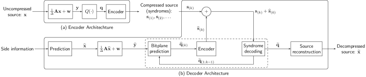
Figure 1: End-to-end high-level architecture and system diagram for (a) the compressor and (b) the decompressor.

III-A1 Measurement and Quantization

In the first stage, the encoder generates measurements $\mathbf{y}\in\mathbb{R}^{m}$ according to

$$\mathbf{y}=\frac{1}{\Delta}\mathbf{A}\mathbf{x}+\mathbf{w},$$ (6)

where $\mathbf{A}\in\mathbb{R}^{m\times n}$ is a measurement operator, $\Delta\in\mathbb{R}^{+}$ is a scaling parameter, and the vector $\mathbf{w}\in\mathbb{R}^{m}$ is a randomized dither with i.i.d. elements drawn uniformly in $[-1,0)$. The measurement parameters, $\Delta$, $\mathbf{A}$, and $\mathbf{w}$, are also available at the decoder.

The acquired measurements are quantized element-wise, using a $B$-bit scalar uniform integer quantizer $Q(\cdot)$. Quantization produces the quantized measurements $\mathbf{q}\in\mathbb{Z}^{m}$, with the $i^{\mathrm{th}}$ quantized measurement given by

$$\mathbf{q}_{i}=Q(\mathbf{y}_{i})=\left\lfloor\mathbf{y}_{i}+\frac{1}{2}\right\rfloor.$$ (7)

We assume that $B$ is selected sufficiently large, such that the quantizer does not saturate.

Since the quantizer rounds to the nearest integer, the scaling parameter $\Delta$ is equivalent to an effective quantization interval on unscaled measurements. Thus, the choice of $\Delta$ affects the reconstruction quality and the bit budget needed to encode $\mathbf{x}$. In particular, reducing $\Delta$ results in finer measurement quantization and, thus, improved reconstruction, at the cost of higher encoding rate. Note that particular rate points can be chosen simply by looking at the data and choosing $\Delta$ at the encoder, without a need for decoding. Furthermore, the random dither $\mathbf{w}$ ensures that the quantization error is uniformly distributed, i.e., $\left(Q(\mathbf{y}_{i})-\mathbf{y}_{i}\right)\stackrel{{\scriptstyle i.i.d}}{{\sim}}\mathcal{U}[-\frac{1}{2},\frac{1}{2})$ for $i=1,\dots,m$ [46], a property that facilitates the analysis necessary to determine the appropriate rate to use in encoding each syndrome.

III-A2 Syndrome Generation

In order to encode and generate syndromes for the quantized measurements, we first separate them into distinct bitplanes. In particular, we use $\mathbf{q}_{(k)}$, $k=1,\ldots,B$, to denote the $k^{\mathrm{th}}$ bitplane of the quantized measurements. We use the convention that $k=1$ and $k=B$ respectively represent the least significant bit (LSB) plane and the most significant bit (MSB) plane. The binary representation of $\mathbf{q}$ can be thought of as an $m\times B$ binary matrix whose $k^{\mathrm{th}}$ column, $\mathbf{q}_{(k)}\in\mathbb{F}_{2}^{m},$ is a binary vector containing the $k^{\mathrm{th}}$ significant bit of all $m$ quantized measurements of $\mathbf{x}$. The following is an example of the above described bitplane representation with $m=3$ and $B=4$:

$$\mathbf{q}=\left(\begin{array}[]{c}3\\ 0\\ 1\end{array}\right)\overset{\mathbb{F}_{2}}{\Longrightarrow}\blockarray{cccc}\mathbf{q}_{(4)}&\mathbf{q}_{(3)}\mathbf{q}_{(2)}\mathbf{q}_{(1)}\\ \block{(cccc)}0011\\ 0000\\ 0001\\ .$$

For each bitplane $\mathbf{q}_{(k)}$ the encoder generates a syndrome at a specific rate. The rate is different for each bitplane and is based on the expected number of errors in this bitplane that will need to be corrected. The syndromes are used by the decoder to correct these errors and reconstruct $\mathbf{x}$ via the iterative decoding procedure outlined in Section III-B.

In particular, for each bitplane, $\mathbf{q}_{(k)}$, the encoder assumes that the decoder has an estimate of the bitplane, $\widehat{\mathbf{q}}_{(k)}$ with a few errors, i.e., bitflips. This estimate is computed at the decoder using the side information and the previously corrected bitplanes $1,\ldots,k-1$. The encoder assumes that each bit in this estimate might be flipped with probability $p_{k}$, which is assumed known at the encoder. Thus, as described in Sec. II-A, the prediction acts as a binary symmetric channel with crossover probability $p_{k}$. The encoder can efficiently encode $\mathbf{q}_{(k)}$ by transmitting a syndrome that corrects the bitflips in the predicted bitplane, i.e., using a code with rate lower than:

$$C_{\mathrm{BSC}-(p_{k})}=1-H_{\mathrm{B}}(p_{k}).$$ (8)

Thus, the encoder uses a parity-check matrix $\mathbf{H}_{(k)}$ with associated rate lower than (8), to allow correction of bitplane prediction errors. In other words, the encoder computes syndromes $\mathbf{s}_{(k)}=\mathbf{H}_{(k)}\mathbf{q}_{(k)}$ for $k=1,\dots,B$ and transmits them to the decoder. In practice, as elaborated in Section IV-D, only few lower significance bitplanes need to be encoded; higher significance ones can be perfectly predicted at the receiver.

Of course, to be able to successfully recover $\mathbf{q}_{(k)}$, it is critical that the encoder accurately determines the probabilities $p_{k}$, or an upper bound for them. The following theorem makes this computation exact, as a function of the $\ell_{2}$ norm of the prediction error, assuming that the measurement matrix $\mathbf{A}$ is drawn from an i.i.d. Gaussian distribution.

Theorem 1.

Consider a signal $\mathbf{x}$ with measurements $\mathbf{y}$ acquired using (6) and quantized to $\mathbf{q}$ using (7), where $\mathbf{A}$ is randomly drawn with i.i.d. $\mathcal{N}(0,\sigma^{2})$ entries. Assume there exists a prediction $\widehat{\mathbf{x}}$, with prediction error $\epsilon=\|\mathbf{x}-\widehat{\mathbf{x}}\|_{2}$ and that the first $k-1$ least significant bitplanes of $\mathbf{q}$, namely $\mathbf{q}_{(i)},i=1,\ldots,k-1$, are perfectly known. Then $\mathbf{q}_{(k)}$, the $k^{\mathrm{th}}$ bitplane of $\mathbf{q}$, can be estimated from $\widehat{\mathbf{x}}$ and $\mathbf{q}_{(i)},i=1,\ldots,k-1$ with bit error probability equal to

$$p_{k} =\frac{1}{2}-\sum_{l=1}^{+\infty}e^{-\frac{1}{2}\left(\frac{\pi\sigma\epsilon l}{2^{k-1}\Delta}\right)^{2}}\mathrm{sinc}\left(\frac{l}{2^{k}}\right)\mathrm{sinc}\left(\frac{l}{2}\right).$$ (9)

Proof:

See Appendix A. ∎

As detailed in the proof, this error probability can be achieved using the decoding method described in Sec. III-B below. Fig. 2(a) plots the theoretical and empirical bit error probabilities for bit $k=3$. The theoretical values are calculated using Thm. 1 as a function of the prediction error $\epsilon=\|\mathbf{x}-\widehat{\mathbf{x}}\|_{2}$. The empirical values are calculated as $m^{-1}\|\mathbf{q}_{(3)}-\widehat{\mathbf{q}}_{(3)}\|_{0}$, where $\mathbf{q}_{(3)}$ and $\widehat{\mathbf{q}}_{(3)}$ correspond to the third bitplane of the quantized measurements of $\mathbf{x}$ and $\widehat{\mathbf{x}}$, respectively, generated from synthetic data such that $\epsilon=\|\mathbf{x}-\widehat{\mathbf{x}}\|_{2}$. As evident in the figure, the empirical probabilities closely match the ones predicted by Thm. 1.

Note that, even if the prediction error is not known but can be upper bounded, the theorem provides an upper bound on the probability of bitflips. Furthermore, as we discuss in Sec. IV, the theorem can be used to provide guidance even if other, more practical, measurement matrices are used.

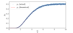
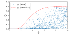
(a) (b) (c)

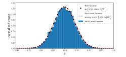
Figure 2: Empirical and theoretical bit error probabilities for quantized measurements as a function of the normalized prediction error $\frac{\epsilon\sigma}{\Delta}$ for $k=3$, (a) acquired using a Gaussian matrix, and (b) acquired using a SRHT operator. (c) Histogram of measurements acquired using the SRHT operator, a Gaussian fit using the empirical mean and variance of the measurements and the equivalent Gaussian sensing matrix statistics.

III-B Decoding

The decoder, shown in Fig. 1(b), uses the syndromes $\mathbf{s}_{(k)}$ of the quantized measurement bitplanes $\mathbf{q}_{(k)}$ and the side information to recover the quantized measurements and reconstruct the signal. Decoding, or decompression, consists of:

• Measurement prediction from the side information.

• Recovery of the original quantized measurements via iterative bitplane prediction and syndrome decoding.

• Source reconstruction from the quantized measurements.

III-B1 Prediction and Measurement

First, the decoder generates a prediction $\widehat{\mathbf{x}}$ of the source $\mathbf{x}$ using the side information and measures the prediction using the same measurement parameters $\mathbf{A},\Delta$, and $\mathbf{w}$ as used by the encoder:

$$\widehat{\mathbf{y}}=\frac{1}{\Delta}\mathbf{A}\widehat{\mathbf{x}}+\mathbf{w}.$$ (10)

III-B2 Recovery of Quantized Measurements

Next, the decoder reconstructs the original quantized measurements $\mathbf{q}$ one bitplane at a time, starting from the least significant bitplane. For the recovery of each bitplane, the decoder uses all the previously recovered bitplanes and the predicted measurements $\widehat{\mathbf{y}}$. As illustrated in Fig. 3, each syndrome-encoded bitplane $k$ is recovered via a two-stage scheme: bitplane prediction followed by syndrome decoding.

The quantized measurements are iteratively recovered starting with the least significant bitplane $k=1$. At iteration $k$, a new estimate of the quantized measurements $\widehat{\mathbf{q}}$ is computed using bitplane prediction, incorporating all the already decoded information from previous iterations. From that estimate, the $k^{\mathrm{th}}$ bitplane, $\widehat{\mathbf{q}}_{(k)}$, is predicted and then corrected using the syndrome $\mathbf{s}_{(k)}$, to recover the corrected bitplane $\widetilde{\mathbf{q}}_{(k)}$. If the syndrome rate has been correctly chosen, decoding is successful with high probability and $\widetilde{\mathbf{q}}_{(k)}=\mathbf{q}_{(k)}$.

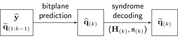
Figure 3: Recovering quantized measurements of bitplane $k$ from the predicted measurements $\widehat{\mathbf{y}}$ and the previously recovered $k-1$ bits $\widetilde{\mathbf{q}}_{(1:k-1)}$.

Specifically for $k=1$, the decoder estimates the quantized measurements $\overline{\mathbf{q}}=Q(\widehat{\mathbf{y}})$ and extracts the least significant bitplane $\widehat{\mathbf{q}}_{(1)}=\overline{\mathbf{q}}_{(1)}$. The corrected least significant bitplane, $\widetilde{\mathbf{q}}_{(1)}$, is obtained by correcting the mismatch between $\widehat{\mathbf{q}}_{(1)}$ and $\mathbf{q}_{(1)}$ using the syndromes $\mathbf{s}_{(1)}$ and $\widehat{\mathbf{s}}_{(1)}=\mathbf{H}_{(1)}\widehat{\mathbf{q}}_{(1)}$. For the remaining bitplanes, $k>1$, assuming $k-1$ bitplanes have already been successfully decoded, $\widehat{\mathbf{q}}$ is estimated by selecting the uniform quantization interval consistent with the decoded $k-1$ bitplanes and closest to the prediction $\widehat{\mathbf{y}}$. Having correctly decoded the first $k-1$ bitplanes is equivalent to the signal being encoded with a $(k-1)$-bit universal quantizer [38]. Thus, recovering $\widetilde{\mathbf{q}}$ uses the same decoding as in [9].

An example of $k-1=2$ is shown in Fig. 4. The left hand side of the figure plots a 2-bit universal quantizer, equivalent to a uniform scalar quantizer with all but the 2 least significant bits dropped. The right hand side shows the corresponding 3-bit uniform quantizer used to produce $q$. In this example, the two least significant bits decode to the universal quantization value of 1, which could correspond to $q=1$ or $-3$ in the uniform quantizer. However, the prediction of the measurement $\widehat{y}$ is closer to the interval corresponding to $q=-3$, and, therefore $\widehat{q}=-3$ is recovered. For a formal description of the bitplane prediction process see Appendix A.

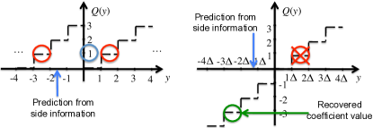
Figure 4: Bitplane prediction of a quantization point using the prediction measurement.

After the $k^{\mathrm{th}}$ bitplane is estimated, the estimate $\widehat{\mathbf{q}}_{(k)}$ is corrected via syndrome decoding of $\mathbf{s}_{(k)}$ and $\widehat{\mathbf{s}}_{(k)}$ to produce the corrected estimate $\widetilde{\mathbf{q}}_{(k)}$. As long as the syndromes satisfy the rate conditions of Thm. 1, decoding is reliable and $\widetilde{\mathbf{q}}_{(k)}=\mathbf{q}_{(k)}$.

Decoding continues iteratively until all $B$ bitplanes have been correctly decoded. Reliable decoding at every iteration guarantees that the decoded quantized measurements are equal to the encoded quantized measurements, i.e., $\widetilde{\mathbf{q}}=\mathbf{q}$. The described syndrome coding procedure bears conceptual similarity to multilevel coding schemes where information is encoded using a number of channel codes of different rates and decoding proceeds in a multistage fashion where each bitplane, starting from the LSB, is decoded by incorporating information from preceding stages [47]. We note that, although in theory the decoding order of the bitplanes should not matter—as long as the encoding provides the correct syndrome rates given this order, and the decoder is able to exploit all statistical dependencies—decoding from least to most significant bit can reduce the number of bitplanes that need to be coded. In practice, this reduces the rate overhead due to finite block lengths and other practical considerations.

We should also note that a common assumption in such schemes is that decoding is successful in each stage before decoding the next. Incorrect decoding of one stage will degrade the bitplane prediction for the next stage and affect the probability of correct decoding. Since the probability of incorrect decoding can, in principle, become arbitrarily low using good codes of the correct rates, the probability of failing to decode any of the $B$ bitplanes can be easily controlled using a union bound on the probability of failure to decode each bitplane separately. A careful analysis of the effects of incorrect prediction on the error probability at the next bit level could be performed using the tools used in proving Theorem 1. However, such an analysis is beyond the scope of this work.

III-B3 Source Reconstruction

The decoder solves an inverse problem to reconstruct the source from the recovered quantized measurements $\widetilde{\mathbf{q}}=\mathbf{q}$, as described in Sec. II-B:

$$\widetilde{\mathbf{x}}=\arg\min_{\mathbf{x}}~{}\mathcal{D}\left(\widetilde{\mathbf{q}},\frac{1}{\Delta}\mathbf{A}\mathbf{x}+\mathbf{w}\right)+\lambda\mathcal{R}(\mathbf{x}).$$ (11)

The regularizer $\mathcal{R}(\cdot)$ may exploit the side information, such as the prediction’s sparsity pattern, to improve the signal model.

IV Implementation Considerations

IV-A Efficient Measurements Operators

Using a Gaussian matrix for encoding, as assumed in Thm. 1, may prove challenging particularly when the encoder is implemented in finite-precision arithmetic with limited memory and computation. Instead, most practical implementations will use measurement approaches based on fast transforms [48], some of which have been shown to satisfy the restricted isometry property (RIP) or have other properties desirable for measurement systems. These approaches exploit the fast transform structure to reduce computation and storage to $\mathcal{O}(n\log n)$ and $\mathcal{O}(n)$, respectively, instead of $\mathcal{O}(nm)$.

Approaches based on the Walsh–Hadamard transform (WHT) are particularly appealing, as the transform only uses addition and subtraction operations, and no multiplications. Similarly to the approach used in [49], we measure by applying a random permutation to the signal $\mathbf{x}$, applying the WHT and randomly subsampling the output. We denote this SRHT, although it is slightly different than the SRHT in [50], in that our approach does not multiply the signal with a random diagonal $\pm 1$ operator before the permutation.

The histogram in Fig. 2(c) illustrates that our SRHT measurements behave similarly to measurements of the same signal using a Gaussian matrix that satisfies Thm. 1 conditions. Fig. 2(b) further suggests empirically that the bit error probability computed in Thm. 1 overestimates $p_{k}$, when the SRHT is used—we conjecture it is an upper bound. Thus, it seems reasonable to use (9) in this case, something we confirmed in our experiments in Section V.

IV-B Binary Representation

To represent the quantized measurements, we use an offset-binary representation. In other words, all measurements are made positive before quantization by an appropriate constant shift that can be removed in decoding. This representation produces quantization intervals that are uniform in all bitplanes. Furthermore, combined with the randomized measurements and our choice of dither, this representation produces uniform $\{0,1\}$ bit distribution in all bitplanes, which is important in designing the syndromes. A two’s complement binary representation has similar properties and could be used instead.

In contrast, sign-magnitude and one’s complement representations have two different binary strings representing zero; a positive and a negative one. These require special handling, and make the representation more cumbersome and slightly less efficient. In addition, such representations might introduce bias and correlations on the bit distribution in each bitplane.

IV-C Efficient Channel Codes

In order to maximize the syndrome-based compression, a rate-efficient channel code must be used to generate syndromes. One popular choice are low-density parity-check (LDPC) codes which are capacity-approaching, and hence allow high compression rates. LDPC codes are particularly appealing because their extremely sparse parity-check matrices allow syndrome generation with complexity $\sim\mathcal{O}(m)$, rather than $\mathcal{O}(m^{2})$. Furthermore, the sparsity enables simple efficient decoding using belief propagation.

Decoding using belief propagation is initialized using prior likelihoods associated with each of the bits to be decoded, reflecting the prior probability of a certain bit taking the value 0 versus 1. In our case, the likelihood corresponds to the probability that the predicted bit in question will be in error (when compared to the same bit of the measured signal). A simple agnostic option is to set the likelihood for all the bits of a given bitplane $k$ to its associated bitflip probability $p_{k}$. Since the bits in each bitplane are uniformly distributed by design, as described above, it is not necessary to adjust this prior, as described, for example, in [51, 52].

In addition, the prediction process in Fig. 4 provides more information that can be used to improve this likelihood estimate individually, for each bit in the bitplane, using the predicted measurements, $\widehat{\mathbf{y}}$, according to the following theorem.

Theorem 2.

Consider a signal $\mathbf{x}$ that is measured and quantized in the same manner as described in Thm. 1. Assume there exists a prediction $\widehat{\mathbf{x}}$, with prediction error $\epsilon=\|\mathbf{x}-\widehat{\mathbf{x}}\|_{2}$, and let $y$ and $\widehat{y}$ denote single measurements of $\mathbf{x}$ and $\widehat{\mathbf{x}}$, respectively. Assume also that the first $k-1$ least significant bits of $Q(y)$, namely $q_{(i)},i=1,\ldots,k-1$, are perfectly known. Then, the likelihood of error in $\widehat{q}_{(k)}$, the $k^{\mathrm{th}}$ bit of $Q(\widehat{y})$, can be estimated from $\widehat{y}$ and $q_{(i)},i=1,\ldots,k-1$, as

$$L_{k} =\mathrm{Pr}\left(\widehat{q}_{(k)}\neq q_{(k)}\mid\widehat{y},q_{(1)},\ldots,q_{(k-1)}\right)$$ (12)

$$=\frac{A_{2}(k,c)}{A_{1}(k,c)+A_{2}(k,c)},$$ (13)

where

$$A_{1}(k,c)$$

$$=\frac{1}{2^{k}}\left(1+2\sum_{l=1}^{+\infty}e^{-\frac{1}{2}\left(\frac{\pi\sigma\epsilon l}{2^{k-1}\Delta}\right)^{2}}\cos\left(\frac{\pi cl}{2^{k-1}}\right)\mathrm{sinc}\left(\frac{l}{2^{k}}\right)\right),$$ (14)

$$A_{2}(k,c)=A_{1}(k,2^{k-1}-c),$$ (15)

and where $c$ is the smallest distance from $\widehat{y}$ to the center of the quantization interval consistent with the $k-1$ LSBs, $q_{(i)},i=1,\ldots,k-1$.

Proof:

See Appendix B. ∎

Fig. 5(a) demonstrates how the error likelihood $L_{k}$ behaves as a function of the distance parameter $c$, for $k=3$ and different values of the normalized prediction error $\frac{\epsilon\sigma}{\Delta}$. As evident, the error likelihood maximum value of 0.5 is attained when $c=\frac{2^{3}}{2}=4$, namely when the prediction $\widehat{y}$ falls exactly in the middle between the two possible consistent quantization intervals (i.e., exactly in between the closest $A_{1}$ and $A_{2}$ regions, in which case $c=\frac{2^{k}}{2}=2^{k-1}$). In that case, the uncertainty in the $k^{\mathrm{th}}$ bit’s predicted value, is maximized, resulting in the maximum likelihood of error.

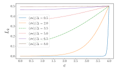
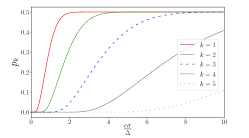
(a) (b) (c)

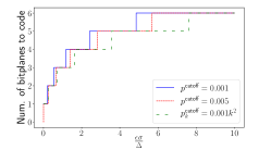
Figure 5: (a) The bit error likelihood $L_{k}$ as a function of the distance parameter $c$ when $k=3$. (b) Bit error probability $p_{k}$ as a function of the normalized prediction error $\frac{\epsilon\sigma}{\Delta}$ for different values of $k$. (c) The number of bitplanes that need to be coded as syndromes as a function of the normalized prediction error $\frac{\epsilon\sigma}{\Delta}$.

As expected, in our simulations we observe that this approach improves the LDPC decoding process. In particular, it allows successful belief propagation using higher code rates, compared to the agnostic prior, which translates to smaller syndrome sizes and hence increased compression rate.

IV-D Cutoff Probabilities for Syndrome Generation

The behavior of the bit error probability, calculated according to (9), as a function of the normalized prediction error $\frac{\epsilon\sigma}{\Delta}$ for different values of $k$ is shown in Fig. 5(b). As the figure illustrates, the error probability decreases sharply for bitplanes of higher significance. If the error $\epsilon$ is sufficiently small, bitplanes beyond a certain significance can be predicted error-free at the decoder, without the need to transmit syndromes. In practice, it is reasonable to set a cutoff probability $p^{\text{cutoff}}$ below which bitplanes are not encoded.

This cutoff can be chosen in a number of ways. For example, we may choose a fixed probability, e.g., $p^{\text{cutoff}}=0.001$, or one that is reciprocal to the syndrome length, i.e., $p^{\text{cutoff}}\propto 1/m$, where the constant of proportionality is chosen to “control” the expected frequency of bit errors in non-encoded bitplanes. Alternatively, since bitplanes are decoded sequentially from LSB to MSB, we may consider assigning different cutoffs to each bitplane, to prevent error propagation across bitplanes. Cutoffs can therefore be assigned in a progressive manner from lower to higher values, with lower significance bits treated more conservatively than higher significance bits, e.g., $p_{k}^{\text{cutoff}}=0.001k$ or $p_{k}^{\text{cutoff}}\propto k/m$.

Fig. 5(c) shows the number of bitplanes that need to be encoded as syndromes as a function of the normalized prediction error for three different cutoff probabilities. The $\Delta$ parameter controls the quantizer resolution. Increasing $\Delta$ is equivalent to using a coarser scalar quantizer, which results in higher distortion, but makes bitplanes more predictable. Thus, as the figure shows, fewer bitplanes need to be encoded as $\Delta$ increases, improving the compression rate. Hence, the $\Delta$ parameter, which is one of the algorithm’s design parameters, plays a key role in controlling the rate-distortion trade-off.

For some bitplanes of low significance, the error rate $p_{k}$ is so high, that the syndrome has effectively the same bit-size as the bitplane, i.e., requires a rate 0 code. In those cases it makes more sense to simply transmit the bitplane instead of spending the extra computation to code and decode it without reducing the number of bits. Thus another cutoff can be set in practice for the value of $p_{k}$, above which the bitplane is transmitted as is. This cutoff is not as critical. Setting it lower than necessary makes the compression slightly less efficient, but does not introduce any errors in the iterative process.

For simplicity, we chose a fixed probability for both cutoffs. In our experiments, typically 1 or 2 least significant bitplanes were transmitted as is. At most 3 additional bitplanes were transmitted by syndrome coding at code rates greater than 0 but less than 1. Syndrome coding and transmission of the remaining, higher significance, bitplanes was unnecessary, as they could be reliably recovered at the decoder from the source prediction.

IV-E Encoding Complexity

In general, the computational and storage cost of the linear measurement operation is $\mathcal{O}(nm)$, dominated by the matrix-vector multiplication $\mathbf{A}\mathbf{x}$. However, using a fast-transform-based measurement operator, as described above, the computational cost can reduce to $\mathcal{O}(n\log n)$ and storage to $\mathcal{O}(n)$. The measurements are quantized using an $\mathcal{O}(n)$ scalar quantizer.

The generation of syndromes involves multiplication of the parity-check matrices $\mathbf{H}_{(k)}$ of size $m(1-R_{k})\times m$, where $R_{k}\in\left[0,1\right]$ is the code rate used to encode the $k^{\mathrm{th}}$ bitplane, by the vectors of quantized measurements $\mathbf{q}_{(k)}$ of size $m$. The worst case complexity, when $R\approx 0$, is order $\mathcal{O}(m^{2})$. However, in practice, structured parity-check matrices can be used to generate syndromes more efficiently, with complexity as low as $\mathcal{O}(m)$. Obtaining the required code rates $R_{k}$ involves calculating the bit error probabilities $p_{k}$ according to Thm. 1, which can be done in constant time.

In summary, complexity is dominated by an $\mathcal{O}(n\log n)$ matrix-vector multiplication. Furthermore, the end-to-end encoder architecture is very simple, as typical in distributed coding schemes, and can be efficiently implemented in resource-constrained environments. Instead the complexity has been transferred to the decoder, which has the ability to exploit signal models through the prediction and the regularization process, even if these signal models are too expensive to be computed at the encoder.

V Application: Multispectral Image Compression

As an example use of our approach, we demonstrate its application to lightweight multispectral image compression targeted to on-board satellite systems.

Multispectal images comprise of four to eight spectral bands, which are typically highly correlated. Such images are often acquired on board satellites for remote sensing applications such as mineral exploration, surveillance and cartography. Advances in modern sensing technology have resulted in increases in the resolution and quality of the sensing instruments, with a corresponding increase in the data size. Thus, considering the communication constraints in space, compression has become a necessity for such systems. Furthermore, resource constraints make existing transform coding-based approaches, such as JPEG-2000, unsuitable. Hence, there is significant interest in rate-efficient compression algorithms with low-complexity encoders. For example, some low-complexity multispectral compression methods can be found in [7, 8, 53, 54, 9, 40].

The approach we present here expands on the approach in [10], by incorporating likelihood estimation in syndrome decoding and further exploiting inter-band correlations using successive prediction from already decoded bands. Consistent with [7, 8, 9, 40], we consider images comprising of four spectral bands $\mathbf{x}_{0},\ldots,\mathbf{x}_{3}$, corresponding to blue, green, red and infrared, respectively. We assume that the blue band, $\mathbf{x}_{0}$, is fully available at the decoder as side information and we explore the compression of the remaining three spectral bands. The approach we present can be naturally generalized to the compression of multiple correlated sources in other modalities.

V-A Encoding

To encode the images, we first separate them to non-overlapping blocks of size $n=64\times 64$, which are treated and compressed independently using the system in Fig. 6(b). Each block is measured with $m=4000$ measurements for each image band, $\mathbf{x}_{i},i=1,2,3$, according to (6), using the SRHT and an appropriate choice of $\Delta$ to achieve the desired rate. Preliminary experiments demonstrated that very low undersampling, with $m=4000$, provided better rate-distortion performance and allowed for better rate-distortion control through the choice of $\Delta$. This is consistent with some of the findings in [55]. The measurements are quantized with a $B=11$ bits scalar quantizer.

Figure 6: End-to-end system for the compression of a multispectral image. The source image (a) is compressed by the encoder (b) to produce syndromes and side information. The decoder (c) decodes the syndromes using the side information to produce the decompressed image (d).

In addition to syndromes, the encoder calculates statistics—specifically, the mean and variance of each band, and the covariance with the other bands—which are communicated to the decoder as part of the side information. These statistics allow the encoder to estimate the prediction error and determine the appropriate rate point for the syndromes. The statistics also enable the decoder to predict the source.

Due to the complexity of generating codes at arbitrary rates during operation, we maintain and select codes from a database of LDPC codes corresponding to rates $0.05,0.1,\dots,0.95$ of block length $m=4000$, stored on-board. Due to the effects of finite block lengths, to ensure accurate decoding, we heuristically back off and select a code with rate $0.05$ lower than the one closest to capacity. For example, if for some bitplane $k$ the error probability is $p_{k}=0.11$, the resulting channel capacity is $C=0.5$ and we select code rate $0.45$ to encode. Using this heuristic, we observed that belief propagation converged almost always in practice, with extremely rare failures. Without the back-off, we observed an increase in LDPC decoding errors, leading to deterioration in reconstruction quality.

More sophisticated approaches might improve code rate selection, and resulting performance. For example, recent work on finite blocklength codes derives improved bounds for rate selection [56, 57]. In our experiments, the additional complexity provided limited benefit. However, the benefit might be greater in applications with smaller block lengths.

V-B Decoding

The decoder, shown in Fig. 6(c), uses the syndromes and the side information, i.e., the reference blue band $\mathbf{x}_{0}$ and the signals statistics, to recover the remaining spectral bands.

V-B1 Image Prediction

To predict measurements at the decoder, we explore two approaches of different complexity and predictive power.

Linear Prediction

The simplest approach is to use a linear minimum mean-square error (LMMSE) estimator to predict each of the three bands $\mathbf{x}_{i},i=1,2,3$ from the blue band $\mathbf{x}_{0}$:

$$\widehat{\mathbf{x}}_{i}=\frac{\overline{\sigma}_{\mathbf{x}_{0}\mathbf{x}_{i}}}{\overline{\sigma}_{\mathbf{x}_{0}}^{2}}\left(\mathbf{x}_{0}-\overline{\mu}_{\mathbf{x}_{0}}\mathbbm{1}\right)+\overline{\mu}_{\mathbf{x}_{i}}\mathbbm{1},$$ (16)

where $\mathbbm{1}$ is the all-ones vector. Accordingly, the encoder must calculate and communicate to the decoder the mean of each band and its covariance with the blue band:

$$\overline{\mu}_{\mathbf{x}_{i}} =\frac{1}{n}\sum_{j=1}^{n}(\mathbf{x}_{i})_{j},$$

$$\overline{\sigma}_{\mathbf{x}_{0}\mathbf{x}_{i}} =\frac{1}{n}\sum_{j=1}^{n}\left((\mathbf{x}_{0})_{j}-\overline{\mu}_{\mathbf{x}_{0}}\right)\left((\mathbf{x}_{i})_{j}-\overline{\mu}_{\mathbf{x}_{i}}\right),$$

where $(\mathbf{x}_{i})_{j}$, $j=1,\ldots,4096$, represents the $j^{\mathrm{th}}$ pixel value of the $i^{\mathrm{th}}$ image band. Note that $\overline{\mu}_{\mathbf{x}_{0}}$ and $\overline{\sigma}_{\mathbf{x}_{0}}^{2}$ do not need to be transmitted, as they can be directly calculated at the decoder from $\mathbf{x}_{0}$. The coding overhead due to transmission of these parameters is small. For example, using 16 bits per parameter, the 3 covariances and 3 means require $6\times 16=96$ bits per $64\times 64$ block, an overhead of 0.00781 bits per pixel (bpp).

The prediction error for each band, which is also available at the encoder, is equal to

$$\epsilon_{i}^{2}=\|\mathbf{x}_{i}-\widehat{\mathbf{x}}_{i}\|_{2}^{2}=n\left(\overline{\sigma}_{\mathbf{x}_{i}}^{2}-\frac{\overline{\sigma}_{\mathbf{x}_{0}\mathbf{x}_{i}}^{2}}{\overline{\sigma}_{\mathbf{x}_{0}}^{2}}\right).$$ (17)

Successive Prediction

Since the decoder may recover the measurements of each band one at a time, it has additional information that can be used to predict subsequent bands. For example, the green band is spectrally closer to the red band than the blue band is, so, presumably, a successfully decoded green band contains additional information that can assist in the prediction of the red band. Thus, successive prediction leverages the results of all the previously decoded bands to improve the prediction error.

The source signals $\mathbf{x}_{i}$ are only available approximately at the decoder, with an unknown error that is difficult to quantify due to the non-linearity of the reconstruction process. On the other hand, their quantized measurements $\mathbf{q}_{i}=Q(\mathbf{y}_{i})$ are available exactly, i.e., assuming, as before, that measurement reconstruction is reliable with $\widetilde{\mathbf{q}}_{i}=\mathbf{q}_{i}$, and the quantization error can be exactly quantified thanks to the effects of dither. Thus, the already recovered measurements can be used for prediction and error estimation.

Measurements of band $i$, acquired according to (6), are

$$\mathbf{y}_{i}=\frac{1}{\Delta_{i}}\mathbf{A}\mathbf{x}_{i}+\mathbf{w}_{i}.$$ (18)

Furthermore, we use $\widetilde{\mathbf{y}}_{i}=\mathbf{y}_{i}-\mathbf{w}_{i}$ to denote the pre-dithered measurements, and $\widetilde{\mathbf{y}}_{i}^{q}=Q(\mathbf{y}_{i})-\mathbf{w}_{i}$ to denote the quantized measurements with dither removed after quantization. Since dither coefficients are drawn uniformly in $[-1,0)$, the quantization error $\mathbf{e}_{i}=Q(\mathbf{y}_{i})-\mathbf{y}_{i}=\widetilde{\mathbf{y}}_{i}^{q}-\widetilde{\mathbf{y}}_{i}$ also comprises of i.i.d. coefficients, uniformly distributed in $[-\frac{1}{2},\frac{1}{2})$ [46]. Thus, the quantization error is a random variable $E_{i}$ with mean $\mu_{E_{i}}=0$ and variance $\sigma_{E_{i}}^{2}=\frac{1}{12}$.

Successful decoding of all bitplanes of band $i$, provides the decoder with the quantized measurements $\mathbf{q}_{i}$ and, consequently, $\widetilde{\mathbf{y}}_{i}^{q}$. Instead of linearly predicting the measurements from the blue band only, successive prediction uses the quantized and dither-removed measurements of bands $i=1,\ldots,k-1$, i.e., $\widetilde{\mathbf{y}}_{i}^{q}$, to predict the pre-dithered measurements of band $k$ using a multi-variable LMMSE estimator:

$$\left(\widehat{\widetilde{\mathbf{y}}}_{k}\right)_{j} =C_{k,k-1}^{T}C_{k-1}^{-1}\begin{bmatrix}\left(\widetilde{\mathbf{y}}_{0}\right)_{j}-\overline{\mu}_{\widetilde{\mathbf{y}}_{0}}\\ \left(\widetilde{\mathbf{y}}_{1}^{q}\right)_{j}-\overline{\mu}_{\widetilde{\mathbf{y}}_{1}^{q}}\\ \vdots\\ \left(\widetilde{\mathbf{y}}_{k-1}^{q}\right)_{j}-\overline{\mu}_{\widetilde{\mathbf{y}}_{k-1}^{q}}\end{bmatrix}+\overline{\mu}_{\widetilde{\mathbf{y}}_{k}},$$ (19)

for $j=1,\dots,m$ and where

$$C_{k,k-1}=\begin{bmatrix}\overline{\sigma}_{\widetilde{\mathbf{y}}_{k}\widetilde{\mathbf{y}}_{0}},\overline{\sigma}_{\widetilde{\mathbf{y}}_{k}\widetilde{\mathbf{y}}_{1}^{q}},\dots,\overline{\sigma}_{\widetilde{\mathbf{y}}_{k}\widetilde{\mathbf{y}}_{k-1}^{q}}\end{bmatrix}^{T},$$ (20)

and

$$C_{k-1}=\begin{bmatrix}\overline{\sigma}_{\widetilde{\mathbf{y}}_{0}}^{2}&\overline{\sigma}_{\widetilde{\mathbf{y}}_{0}\widetilde{\mathbf{y}}_{1}^{q}}&\dots&\overline{\sigma}_{\widetilde{\mathbf{y}}_{0}\widetilde{\mathbf{y}}_{k-1}^{q}}\\ \overline{\sigma}_{\widetilde{\mathbf{y}}_{1}^{q}\widetilde{\mathbf{y}}_{0}}&\overline{\sigma}_{\widetilde{\mathbf{y}}_{1}^{q}}^{2}&\dots&\overline{\sigma}_{\widetilde{\mathbf{y}}_{1}^{q}\widetilde{\mathbf{y}}_{k-1}^{q}}\\ \vdots&\vdots&\ddots&\vdots\\ \overline{\sigma}_{\widetilde{\mathbf{y}}_{k-1}^{q}\widetilde{\mathbf{y}}_{0}}&\overline{\sigma}_{\widetilde{\mathbf{y}}_{k-1}^{q}\widetilde{\mathbf{y}}_{1}^{q}}&\dots&\overline{\sigma}_{\widetilde{\mathbf{y}}_{k-1}^{q}}^{2}\end{bmatrix}.$$ (21)

To predict $\mathbf{y}_{k}$ the decoder therefore requires $\mathbf{y}_{0}$ (which is available as side information) and $\mathbf{q}_{1},\dots,\mathbf{q}_{k-1}$ (which are recovered by the decoder prior to predicting $\mathbf{y}_{k}$).

Note that (19) implies that statistical parameters are available for non-quantized measurements (e.g., $\overline{\mu}_{\widetilde{\mathbf{y}}_{k}}$), quantized measurements (e.g., $\overline{\mu}_{\widetilde{\mathbf{y}}_{k-1}^{q}}$) and a mix of both (e.g., $\overline{\sigma}_{\widetilde{\mathbf{y}}_{0}\widetilde{\mathbf{y}}_{1}^{q}}$), which might not always be available at the encoder. However, the dither allows us to compute the statistics of quantized measurements from the non-quantized ones. If $\widetilde{Y}_{i}$ and $\widetilde{Y}_{i}^{q}$ denote the random variables corresponding to the entries of $\widetilde{\mathbf{y}}_{i}$ and $\widetilde{\mathbf{y}}_{i}^{q}$, respectively, then

$$\mu_{\widetilde{Y}_{i}^{q}}=\mathbb{E}{[\widetilde{Y}_{i}^{q}]}=\mathbb{E}{[\widetilde{Y}_{i}+E_{i}]}=\mathbb{E}{[\widetilde{Y}_{i}]}=\mu_{\widetilde{Y}_{i}},$$ (22)

since $E_{i}$ is zero mean, and

$$\sigma_{\widetilde{Y}_{j}^{q}}^{2} =\mathrm{Var}{[\widetilde{Y}_{j}]}+\mathrm{Var}{[E_{j}]}=\sigma_{\widetilde{Y}_{j}}^{2}+\frac{1}{12},$$ (23)

since $E_{j}$ and $\widetilde{Y}_{j}$ are independent. Furthermore,

$$\sigma_{\widetilde{Y}_{i}^{q}\widetilde{Y}_{j}} =\mathbb{E}{[(\widetilde{Y}_{i}+E_{i})\widetilde{Y}_{j}]}-\mathbb{E}{[\widetilde{Y}_{i}^{q}]}\mathbb{E}{[\widetilde{Y}_{j}]}=\sigma_{\widetilde{Y}_{i}\widetilde{Y}_{j}},$$ (24)

and, similarly

$$\sigma_{\widetilde{Y}_{i}^{q}\widetilde{Y}_{j}^{q}} =\mathbb{E}{[(\widetilde{Y}_{i}+E_{i})(\widetilde{Y}_{j}+E_{j})]}-\mathbb{E}{[\widetilde{Y}_{i}^{q}]}\mathbb{E}{[\widetilde{Y}_{j}]}=\sigma_{\widetilde{Y}_{i}\widetilde{Y}_{j}}.$$ (25)

Thus, empirical statistics of quantized measurements can be approximated using statistics of non-quantized measurements:

$$\overline{\mu}_{\widetilde{\mathbf{y}}^{q}}\approx\overline{\mu}_{\widetilde{\mathbf{y}}},~{}~{} ~{}~{}\overline{\sigma}_{\widetilde{\mathbf{y}}^{q}}^{2}\approx\overline{\sigma}_{\widetilde{\mathbf{y}}}^{2}+\frac{1}{12},$$ (26)

$$\overline{\sigma}_{\widetilde{\mathbf{y}}_{i}^{q}\widetilde{\mathbf{y}}_{j}}\approx\overline{\sigma}_{\widetilde{\mathbf{y}}_{i}\widetilde{\mathbf{y}}_{j}},~{}~{} ~{}~{}\overline{\sigma}_{\widetilde{\mathbf{y}}_{i}^{q}\widetilde{\mathbf{y}}_{j}^{q}}\approx\overline{\sigma}_{\widetilde{\mathbf{y}}_{i}\widetilde{\mathbf{y}}_{j}}.$$ (27)

Assuming approximations (26)–(27) are used, the encoder must calculate and communicate to the decoder the set $\{\overline{\mu}_{\widetilde{\mathbf{y}}_{i}},\overline{\sigma}_{\widetilde{\mathbf{y}}_{i}}^{2},\overline{\sigma}_{\widetilde{\mathbf{y}}_{i}\widetilde{\mathbf{y}}_{j}}:i,j=0,1,2,3,i\neq j\}$, except for $\overline{\sigma}_{\widetilde{\mathbf{y}}_{3}}^{2}$, which is not needed, and $\overline{\mu}_{\widetilde{\mathbf{y}}_{0}}$ and $\overline{\sigma}_{\widetilde{\mathbf{y}}_{0}}^{2}$, which are used but not transmitted because, as before, they can be computed at the decoder. Thus, 11 parameters need to be transmitted, with transmission overhead, assuming again 16 bits per coefficient, equal to $11\times 16=176$ bits, i.e., 0.01432 bpp.

TABLE I: Decoding PSNR at 2 bpp ($512\times 512$ image crop)

	PSNR (dB)				BPP
	green	red	infrared		green	red	infrared	overhead	overall
Benchmark [9]	37.79	32.76	34.24		2.00	2.00	2.00	—	2.00
Linear prediction
Prediction only	33.46	28.53	27.52		—	—	—	—	—
$\Delta_{\mathrm{green}}=\Delta_{\mathrm{red}}=\Delta_{\mathrm{infrared}}=10.395$	39.52	38.89	39.52		1.51	2.19	2.28	0.00781	2.00
$\Delta_{\mathrm{green}}=6.995;\Delta_{\mathrm{red}}=12.275;\Delta_{\mathrm{infrared}}=13$	42.19	38.10	38.15		1.99	1.99	2.00	0.00781	2.00
Successive prediction
$\Delta_{\mathrm{green}}=\Delta_{red}=\Delta_{\mathrm{infrared}}=9.925$	39.79	39.09	39.66		1.55	2.22	2.17	0.01432	2.00
$\Delta_{\mathrm{green}}=7.055;\Delta_{\mathrm{red}}=12.05;\Delta_{\mathrm{infrared}}=11.675$	42.12	38.21	38.92		1.98	1.99	1.98	0.01432	2.00

The encoder can calculate the prediction mean squared error (MSE) to estimate the rates required for the syndromes. The prediction MSE is

$$\mathrm{MSE}_{k} =\frac{1}{m}\|\widehat{\widetilde{\mathbf{y}}}_{k}-\widetilde{\mathbf{y}}_{k}\|_{2}^{2}=\overline{\sigma}_{\widetilde{\mathbf{y}}_{k}}^{2}-C_{k,k-1}^{T}C_{k-1}^{-1}C_{k,k-1}.$$ (28)

The dithered prediction is obtained by adding the dither to the pre-dithered prediction i.e., $\widehat{\mathbf{y}}_{k}=\widehat{\widetilde{\mathbf{y}}}_{k}+\mathbf{w}_{k}$. Thus, the prediction error is

$$\epsilon_{\mathbf{y}_{k}}^{2}=\|\mathbf{y}_{k}-\widehat{\mathbf{y}}_{k}\|_{2}^{2}=\|\widehat{\widetilde{\mathbf{y}}}_{k}-\widetilde{\mathbf{y}}_{k}\|_{2}^{2}.$$ (29)

To calculate the code rates for the syndromes as per Thm.1, we need to determine the distance $\epsilon_{\mathbf{x}_{k}}=\|\mathbf{x}_{k}-\widehat{\mathbf{x}}_{k}\|_{2}$ between a source $\mathbf{x}_{k}$ and its prediction $\widehat{\mathbf{x}}_{k}$. We use the RIP [16] to approximately relate the distance of the measurements and their predictions, $\epsilon_{\mathbf{y}_{k}}$, to $\epsilon_{\mathbf{x}_{k}}$ as follows

$$\epsilon_{\mathbf{x}_{k}}^{2}\approx\frac{n\Delta^{2}}{m}\epsilon_{\mathbf{y}_{k}}^{2}~{}.$$ (30)

Given that $\mathbf{A}$ is almost square and unitary, the RIP constants are very small, so the estimate in (30) is accurate.

TABLE II: Decoding PSNR at 1.68 bpp (full $7040\times 7936$ image)

	PSNR (dB)				BPP
	green	red	infrared		green	red	infrared	overhead	overall
Benchmark [9]	39.06	37.60	35.80		1.68	1.68	1.68	—	1.68
Linear prediction
Prediction only	37.05	31.67	27.32		—	—	—	—	—
$\Delta_{\mathrm{green}}=\Delta_{\mathrm{red}}=\Delta_{\mathrm{infrared}}=9.095$	41.84	41.07	40.08		1.17	1.70	2.15	0.00781	1.68
$\Delta_{\mathrm{green}}=5.225;\Delta_{\mathrm{red}}=9.4;\Delta_{\mathrm{infrared}}=14.385$	44.96	40.89	37.85		1.67	1.67	1.68	0.00781	1.68
Successive prediction
$\Delta_{\mathrm{green}}=\Delta_{\mathrm{red}}=\Delta_{\mathrm{infrared}}=8.7325$	42.08	41.27	40.28		1.20	1.70	2.09	0.01432	1.68
$\Delta_{\mathrm{green}}=5.275;\Delta_{\mathrm{red}}=8.95;\Delta_{\mathrm{infrared}}=13.15$	44.91	41.13	38.32		1.66	1.66	1.66	0.01432	1.68

V-B2 Image Recovery

Once all bitplanes have been successfully decoded, the quantized measurements $\widetilde{\mathbf{q}}_{i},i=1,2,3,$ are used to reconstruct the image by solving the sparse optimization problem (5) with an appropriately chosen data fidelity penalty and regularizer. In our experiments we found that, for our particular rate points of interest with low-distortion, the quadratic penalty performed better than penalties promoting consistent reconstruction. This, however might not be the case if the chosen operating point requires coarser quantization.

In reconstruction, similar to [18], we exploit the presence of the blue reference to weight the regularizer. In particular, we use a total variation (TV)-based regularizer, known to enforce a good model for images by imposing sparsity in their gradient. However, we also expect that if an edge is present in the blue reference band, the edge is likely to be present in the reconstructed band as well, i.e., at the same pixel locations there is going to be a large gradient spike that should not be penalized. To incorporate this additional information on the gradient from the blue reference, we use weighted-TV (WTV),

$$\mathcal{R}_{\mathrm{WTV}}(X)=\\ \sum_{s,t}\sqrt{W_{s,t}^{x}(X_{s,t}-X_{s-1,t})^{2}+W_{s,t}^{y}(X_{s,t}-X_{s,t-1})^{2}},$$ (31)

where $X$ is a 2D image, $W^{x}$ and $W^{y}$ are 2D sets of weights, and $(s,t)$ are image coordinates. Larger weights penalize edges more in the respective location and direction, while smaller weights reduce their significance. When all the weights are set to 1, the regularizer is the standard TV regularizer.

The regularizer weights at pixel spatial coordinate $(s,t)$ are chosen based on the norm of the gradient of the blue reference band at the corresponding pixel, denoted $\Phi(X_{0_{s,t}})$, which is computed using

$$\Phi(X_{0_{s,t}})=\sqrt{(X_{0_{s,t}}-X_{0_{s-1,t}})^{2}+(X_{0_{s,t}}-X_{0_{s,t-1}})^{2}},$$ (32)

where $X_{0_{s,t}}$ is the value of the image pixel of the reference band $\mathbf{x}_{0}$ at coordinate $(s,t)$.

The weights are then computed according to

$$W_{s,t}^{x}=W_{s,t}^{y}=\left\{\begin{array}[]{rl}0.2,&\mathrm{if}~{}\Phi(X_{0_{s,t}})>\tau,\\ 1,&\mathrm{otherwise},\end{array}\right.,$$ (33)

where $\tau=0.3$ is an experimentally tuned threshold, qualifying which gradient norms are considered to be significant and likely to be present in other bands.

To summarize, the decoder solves

$$\widetilde{\mathbf{x}}_{i}=\arg\min_{\mathbf{x}}\bigl{\|}\widetilde{\mathbf{q}}_{i}-\frac{1}{\Delta_{i}}\mathbf{A}\mathbf{x}-\mathbf{w}_{i}\bigr{\|}_{2}^{2}+\lambda\mathcal{R}_{\mathrm{WTV}}(\mathbf{x}),$$ (34)

where $\lambda=0.1$ was tuned experimentally using a small part of the data. Several ways exist to solve (34); we use a fast iterative shrinkage thresholding (FISTA)-based approach [58].

V-C Simulation Results

To measure the performance of our method we consider the trade-off between the compression rate and the quality of reconstruction, measured using the peak signal-to-noise ratio (PSNR) metric. In decibels (dB), PSNR is defined as

$$\text{PSNR}(\mathbf{x}_{i},\widetilde{\mathbf{x}}_{i})=10\log_{10}\left(\frac{\text{max}(\mathbf{x}_{i})^{2}}{\text{MSE}(\mathbf{x}_{i},\widetilde{\mathbf{x}}_{i})}\right),$$ (35)

where $\text{MSE}(\mathbf{x}_{i},\widetilde{\mathbf{x}}_{i})$ is the mean squared error between the source $\mathbf{x}_{i}$ and its reconstruction $\widetilde{\mathbf{x}}_{i}$ and $\text{max}(\mathbf{x}_{i})$ returns the value of the largest element of $\mathbf{x}_{i}$. As a benchmark, we use the results in [9] where a similar complexity encoder was used under the same settings to compress 4-band images acquired by the ALOS satellite [59]. We performed tests on an entire $7040\times 7936$ image, as well as more extensive testing on a smaller $512\times 512$ patch of the same image. This patch, shown in Fig. 6(a), was chosen as it was deemed challenging to compress.

The encoding parameters, $\Delta$ in particular, were chosen to match the rates used in [9]. We considered image blocks of size $n=64\times 64$, and examined the performance under both the simple linear prediction and the successive prediction approaches above. Note that our preliminary work [10] only considers the simple linear prediction approach and does not exploit likelihood computation using Thm. 2 in the decoding.

The results for the compression of the image patch in Fig. 6(a) are reported in Table I. The first row, titled Prediction only, lists the quality of the linear prediction using only side information and prediction parameters, i.e., without syndrome decoding and reconstruction. This quantifies the quality of predicting each band from the reference blue band and serves as a baseline. As expected, the quality of prediction matches the spectral distances between the predicted bands and blue band: the closest green band is easiest to predict, followed by the red band and the furthest infrared band.

We experimented with two different approaches to set the quantization resolution parameter $\Delta$, which controls the rate-distortion trade-off as discussed in Sec. IV-D. In the first approach we chose the same $\Delta$ for all 3 bands, such that the average compression rate is the target of 2 bpp. As expected, the reconstruction quality is fairly similar among the bands, while the bit budget is spread unevenly, with the easier to predict bands requiring lower code rates. In the second approach, the $\Delta$ was set such that each band is compressed at the target rate of 2 bpp. In this case, as expected, the reconstruction quality improves for the easier to predict bands. This improvement comes at the expense of the harder to predict bands, whose reconstruction quality deteriorates. Note that the effectively negligible overhead associated with transmitting the statistical parameters at 16 bits per parameter is included in a separate “overhead” column, and not counted in the calculation of the reported per-band bpp values.

As is apparent from Table I the approach significantly outperforms the benchmark in terms of quality of reconstruction. The ranges of improvements in reconstruction PSNR are summarized in the first two columns of Table III. The performance improvements of linear and successive predictions are quite similar, with successive prediction doing slightly better than linear prediction in most cases.

A similar set of experiments was conducted for the larger $7040\times 7936$ image with a target rate of 1.68 bpp, considering both linear and successive prediction and both fixed and variable $\Delta$. The results are shown in Table II. As expected, the results exhibit a similar behavior to the results of the smaller image patch. A common $\Delta$ for all bands leads to similar reconstruction quality at different compression rates, whereas varying $\Delta$ for each band, such that the rate is the same, leads to variations in reconstruction quality. The performance of the linear and successive prediction is quite similar. As with the smaller image patch, the proposed approach outperforms [9]. The improvements in reconstruction quality are summarized in the two right columns of Table III.

For the large $7040\times 7936$ image, we also examined the quality of reconstructed measurements $\widetilde{\mathbf{q}}_{i}$ with respect to decoding errors. Table IV lists the resulting average bit error rates of $\widetilde{\mathbf{q}}_{i}$, compared to the true $\mathbf{q}_{i}$ for the scenarios we simulated. We observe that the measurements are reliably reconstructed, with bit error rates on the order of $10^{-4}$. This provides some empirical support that our heuristic to accommodate the effects of finite block lengths by choosing slightly conservative code rates, described in Sec. V-A, works well in practice.

TABLE III: Quality improvement over benchmark approach

	$512\times 512$ image			$7040\times 7936$ image
	2.00 bpp			1.68 bpp
Prediction	same $\Delta$	variable $\Delta$		same $\Delta$	variable $\Delta$
Linear	1.7–6.1dB	3.9–5.3dB		2.8–4.3dB	2.0–5.9dB
Successive	2.0–6.3dB	4.3–5.5dB		3.0–4.5dB	2.5–5.9dB

TABLE IV: Average bit error rate of reconstructed measurements (units are $\times 10^{-4}$, for a 7040 $\times$ 7936 image)

	same $\Delta$				variable $\Delta$
Prediction	green	red	infrared		green	red	infrared
Linear	1.01	1.40	1.77		1.71	1.53	1.77
Successive	1.15	1.51	2.00		1.76	1.95	2.00

VI Discussion

The proposed approach exploits advances in sampling theory and signal representations, mostly due to the development of compressed sensing and sparse signal recovery. From this area we inherit several desirable properties, including the universality and the simplicity of the encoder, as well as the ability to incorporate complex signal models and signal dependencies during reconstruction. Because of that, the proposed approach is also future proof: an improvement in signal models can improve decoding performance, without requiring any change in the encoder.

Our development treads at the intersection of quantization, sparse signal processing, and information theory. While we provide a flexible framework for distributed coding, exploiting a modern signal processing paradigm, it is not evident that our approach is in any sense optimal. Optimality in an information-theoretic, rate-distortion sense is, in fact, difficult to quantify. Modern signal models, such as sparsity and structured sparsity, do not fit well the probabilistic information-theoretic framework typically used in deriving optimality bounds. While some progress has been made, e.g., see [23], understanding the information-theoretic properties of such sources is still an open problem and an active area of research. More recently developed learning-based signal models [60] pose even more theoretical questions.

A significant practical advantage of our approach is that the transmission rate can be estimated at the transmitter using only an estimate of the $\ell_{2}$ error at the decoder in Thm. 1. Thus, given a fixed quantization interval $\Delta$, the encoder can easily compute the transmission rate. Furthermore, typically the reconstruction error is expected to be approximately proportional to $\Delta$. A more complex encoder may take this general trend into account, potentially in a rate-distortion optimization component. However, due to the reconstruction’s non-linear nature, the exact relationship between $\Delta$ and the reconstruction error is still not well understood, complicating the development of such a component.

A proper, theoretically-motivated, approach for trading off the values of $m$ and $\Delta$ to achieve a certain rate-distortion trade-off remains an open question of practical importance. While we tuned $m$ empirically in our experiments, a more principled approach is desirable. A rate-distortion function that takes $m$ and $\Delta$ into account would be ideal, but still elusive.

Appendix A Proof of Theorem 1

Proof:

Consider a single measurement of the signal $\mathbf{x}\in\mathbb{R}^{n}$ and its prediction $\widehat{\mathbf{x}}\in\mathbb{R}^{n}$,

$$y=\frac{1}{\Delta}\langle\mathbf{a},\mathbf{x}\rangle+w,~{}\widehat{y}=\frac{1}{\Delta}\langle\mathbf{a},\widehat{\mathbf{x}}\rangle+w,$$ (36)

where $\mathbf{a}\in\mathbb{R}^{n}$ is the measurement vector, $\Delta\in\mathbb{R^{+}}$ is a scaling parameter, $w$ is dither, and $\mathbf{a}$, $\Delta$ and $w$ are common in both measurements. Assume entries of $\mathbf{a}$ are drawn from an i.i.d., $\mathcal{N}(0,\sigma^{2})$ distribution, and $w$ is drawn uniformly in $[-1,0)$. Let

$$Q_{n}(y)=q_{(n)}q_{(n-1)}\dots q_{(1)}$$ (37)

represent the values of the first $n$ LSBs of the quantized measurement $Q(y)$ of $y$.

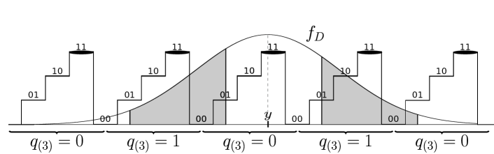
Figure 7: The error probability $p_{3}$ corresponds to the area of the union of inconsistent intervals (shaded).

The decoder predicts $q_{(k)}$ based solely on $\widehat{y}$ and $Q_{k-1}(y)$, which is assumed perfectly known or already correctly decoded. Knowledge of $Q_{k-1}(y)$ is equivalent to knowledge of $y$ quantized using a $(k-1)$-bit universal quantizer [38]. Such a quantizer is equivalent to a uniform scalar quantizer with only the $k-1$ LSBs preserved, i.e., one with $2^{k-1}$ distinct levels, which repeat every $2^{k-1}$ quantization intervals. An example $2$-bit universal quantizer is shown in Fig. 7. The value of the third bit, $q_{(3)}$, alternates every $2^{2}=4$ quantization intervals.

Let $\mathcal{I}_{Q_{k-1}(y)}$ denote the set of all quantization intervals that map to $Q_{k-1}(y)$, that is

$$\mathcal{I}_{Q_{k-1}(y)}=\{\left[a,b\right)\mid Q_{k-1}(t)=Q_{k-1}(y)~{}\forall t\in\left[a,b\right)\}.$$ (38)

Similarly, $\mathcal{I}_{0Q_{k-1}(y)}~{}(\mathcal{I}_{1Q_{k-1}(y)})$ naturally extends the above definition for the case when the $k^{\mathrm{th}}$ bit is $0~{}(1)$. In Fig. 7, $Q_{2}(y)=11$ therefore $\mathcal{I}_{Q_{k-1}(y)}=\mathcal{I}_{11}$ corresponds to the union of all the intervals shown in bold ellipses, while $\mathcal{I}_{0Q_{k-1}(y)}=\mathcal{I}_{011}$ corresponds to the union of the intervals shown in bold ellipses only in the non-shaded regions.

To generate a prediction $\widehat{q}_{(k)}$ of $q_{(k)}$, the decoder first finds the interval $\mathcal{I}^{\star}\in\mathcal{I}_{Q_{k-1}(y)}$ with midpoint closest to $\widehat{y}$:

$$\mathcal{I}^{\star}=\underset{\mathcal{I}\in\mathcal{I}_{Q_{k-1}(y)}}{\mathrm{argmin}}\left|\widehat{y}-\frac{\sup(\mathcal{I})+\inf(\mathcal{I})}{2}\right|.$$ (39)

The decoder then assigns $\widehat{q}_{(k)}$ the value associated with the $k$-bit quantization interval which contains $\mathcal{I}^{\star}$, that is

$$\widehat{q}_{(k)}=\begin{cases}0&\text{if }\exists\widetilde{\mathcal{I}}\in\mathcal{I}_{0Q_{k-1}(y)}\text{ such that }\mathcal{I}^{\star}\subset\widetilde{\mathcal{I}}\\ 1&\text{otherwise }\end{cases}.$$ (40)

This bitplane prediction process is illustrated in Fig. 7. If $\widehat{y}$ is inside the shaded regions, it will be closest to an interval $\mathcal{I}^{\star}\in\mathcal{I}_{Q_{2}(y)}=\mathcal{I}_{11}$ which is contained in an interval of $\mathcal{I}_{1Q_{2}(y)}=\mathcal{I}_{111}$, thus predicting $\widehat{q}_{(3)}=1$. Similarly, if $\widehat{y}$ is inside a non-shaded region, the decoder assigns $\widehat{q}_{(3)}=0$.

For a given $y$, we call intervals of $\mathbb{R}$ which would result in the $k^{\mathrm{th}}$ bit of $\widehat{y}$ to be mapped to $\widehat{q}_{(k)}=q_{(k)}$, consistent intervals. The width of any consistent interval is $2^{k-1}$ and the distance from its center to the center of a neighboring consistent interval is $2^{k}$. In Fig. 7, consistent intervals correspond to the non-shaded regions, each of which has a width of $2^{2}=4$. The union of all consistent intervals $\mathcal{C}(y)$ is given by

$$\mathcal{C}(y) =\lfloor y+\frac{1}{2}\rfloor+\bigcup\limits_{l\in\mathbb{Z}}\left[-2^{k-2}+l2^{k},l2^{k}+2^{k-2}\right].$$ (41)

The signed distance of the measurements, $D$, is defined as

$$D=y-\widehat{y}=\frac{1}{\Delta}\langle\mathbf{a},\mathbf{x}-\widehat{\mathbf{x}}\rangle=\frac{1}{\Delta}\sum_{i=1}^{n}\mathbf{a}_{i}\left(\mathbf{x}_{i}-\widehat{\mathbf{x}}_{i}\right),$$ (42)

where $\mathbf{a}_{i},\mathbf{x}_{i}$ and $\widehat{\mathbf{x}}_{i}$ denote the $i^{\mathrm{th}}$ element of the $\mathbf{a},\mathbf{x}$ and $\widehat{\mathbf{x}}$ vectors, respectively. Since $D$ is a linear combination of $n$ independent Gaussian random variables, it is also a random variable with Gaussian distribution with mean equal to

$$\mathbb{E}{\left[D\right]}=\mathbb{E}{\left[\frac{1}{\Delta}\sum_{i=1}^{n}\mathbf{a}_{i}\left(\mathbf{x}_{i}-\widehat{\mathbf{x}}_{i}\right)\right]}=\frac{1}{\Delta}\sum_{i=1}^{n}\mathbb{E}{\left[\mathbf{a}_{i}\right]}\!\left(\mathbf{x}_{i}-\widehat{\mathbf{x}}_{i}\right)=0,$$ (43)

where we recall that the $\mathbf{x}$ and $\widehat{\mathbf{x}}$ are arbitrary, non-random, vectors. The variance of $D$ equals

$$\mathrm{Var}{\left(D\right)} =\mathbb{E}{\left[D^{2}\right]}=\frac{1}{\Delta^{2}}\mathbb{E}{\left[\left(\sum_{i=1}^{n}\mathbf{a}_{i}\left(\mathbf{x}_{i}-\widehat{\mathbf{x}}_{i}\right)\right)^{2}\right]}$$ (44)

$$=\frac{1}{\Delta^{2}}\sum_{i=1}^{n}\mathbb{E}{\left[\mathbf{a}_{i}^{2}\right]}\left(\mathbf{x}_{i}-\widehat{\mathbf{x}}_{i}\right)^{2}=\left(\frac{\sigma\epsilon}{\Delta}\right)^{2}.$$ (45)

In other words, $D\sim\mathcal{N}\left(0,\left(\frac{\sigma\epsilon}{\Delta}\right)^{2}\right)$ and $f_{D}(\cdot)$ denotes its probability density function (pdf).

For a given $y$, the probability that $\widehat{q}_{(k)}=q_{(k)}$ is the probability that $\widehat{y}\in\mathcal{C}(y)$. This probability can be determined by integrating $f_{D}(\cdot)$ over the coset $\mathcal{C}(y)-y$ as follows:

$$\Pr(\widehat{q}_{(k)}=q_{(k)}\mid y)=\int\limits_{u\in\mathcal{C}(y)-y}f_{D}(u)du.$$ (46)

In order to evaluate (46), we introduce the function $g(\cdot)$, which is a rectangular function of width $2^{k-1}$, repeated at intervals of $2^{k}$, defined as

$$g(u)=\mathrm{rect}\left(\frac{u}{2^{k-1}}\right)\ast\sum_{l=-\infty}^{\infty}\delta\left(u-l2^{k}\right),$$ (47)

where $\delta(\cdot)$ is the Dirac delta function, $\ast$ is the convolution operator on a pair of functions $f$ and $h$ defined as

$$\left(f\ast h\right)\left(u\right)=\int_{-\infty}^{\infty}f\left(\tau\right)h\left(u-\tau\right)d\tau$$ (48)

and $\mathrm{rect}\left(\cdot\right)$ is the rectangular function of unit width and height

$$\mathrm{rect}\left(u\right)=\begin{cases}0&\text{for }\left|u\right|>\frac{1}{2}\\ 1&\text{for }\left|u\right|\leq\frac{1}{2}\end{cases}.$$ (49)

Noting that the support of $g(u-\lfloor y+\frac{1}{2}\rfloor)$ is exactly equal to $\mathcal{C}(y)$, we evaluate (46) as

$$\Pr(\widehat{q}_{(k)}=q_{(k)}\mid y)=\int_{-\infty}^{\infty}f_{D}\left(u\right)g\left(u-t\right)du,$$ (50)

where $t=\lfloor y+\frac{1}{2}\rfloor-y$. Note that the value of $t$ (rather than direct knowledge of $y$) suffices for evaluation of the right-hand side of (50), so we can equivalently write $\Pr(\widehat{q}_{(k)}=q_{(k)}\mid y)=\Pr(\widehat{q}_{(k)}=q_{(k)}\mid t)$ i.e.,

$$\Pr(\widehat{q}_{(k)}=q_{(k)}\mid t)=\int_{-\infty}^{\infty}f_{D}\left(u\right)g\left(u-t\right)du,$$ (51)

As $y$ is a random variable and not known at the decoder, $t$ is also a random variable. Due to the additive dither $w$, the position of $y$ is uniformly distributed across the quantization interval and therefore $t$ is distributed uniformly in $\left[-\frac{1}{2},\frac{1}{2}\right]$[46]. Thus, the pdf of $t$ is $f_{t}\left(\cdot\right)=\mathrm{rect}(\cdot)$.

To determine the probability that $\widehat{q}_{(k)}=q_{(k)}$, we marginalize out the dependence in (51) on $t$ i.e.,

$$\Pr \left(\widehat{q}_{(k)}=q_{(k)}\right)=\int_{-\frac{1}{2}}^{\frac{1}{2}}\Pr\left(\widehat{q}_{(k)}=q_{(k)}\mid\tau\right)f_{t}\left(\tau\right)d\tau$$ (52)

$$=\int_{-\infty}^{\infty}\left[\int_{-\infty}^{\infty}f_{D}\left(u\right)g\left(u-\tau\right)du\right]f_{t}\left(\tau\right)d\tau$$ (53)

$$=\int_{-\infty}^{\infty}f_{D}\left(u\right)\left[\left(g\ast f_{t}\right)(u)\right]du$$ (54)

$$=\int_{-\infty}^{\infty}\mathcal{F}\left\{f_{D}\left(u\right)\right\}\left[\mathcal{F}\left\{g\left(u\right)\right\}\mathcal{F}\left\{f_{t}\left(u\right)\right\}\right]d\xi,$$ (55)

where in (53) we note that the support of $f_{t}(\cdot)$ is only $\left[-\frac{1}{2},\frac{1}{2}\right]$, and in (55) $\mathcal{F}\left\{\cdot\right\}$ denotes the Fourier transform, defined as

$$\mathcal{F}\left\{x\left(u\right)\right\}=\int_{-\infty}^{\infty}x\left(u\right)e^{-j2\pi\xi u}d\xi.$$ (56)

Line (55) follows from the equivalence of convolution in time with multiplication in frequency and Plancherel’s theorem. The Fourier transforms of the functions in (55) equal

$$\mathcal{F}\left\{f_{D}\left(u\right)\right\}=\mathcal{F}\left\{\frac{1}{\sqrt{2\pi\left(\frac{\sigma\epsilon}{\Delta}\right)^{2}}}e^{-\frac{u^{2}}{2\left(\frac{\sigma\epsilon}{\Delta}\right)^{2}}}\right\}=e^{-2\left(\frac{\pi\sigma\epsilon\xi}{\Delta}\right)^{2}},$$ (57)

$$\mathcal{F}\left\{f_{t}\left(u\right)\right\}=\mathcal{F}\left\{\mathrm{rect}(u)\right\}=\mathrm{sinc}\left(\xi\right),$$ (58)

where $\mathrm{sinc}\left(u\right)=\frac{\sin(\pi u)}{\pi u}$ is the normalized sinc function, and

$$\mathcal{F} \left\{g\left(u\right)\right\}=\mathcal{F}\left\{\mathrm{rect}\left(\frac{u}{2^{k-1}}\right)\ast\sum_{l=-\infty}^{+\infty}\delta\left(u-l2^{k}\right)\right\}$$ (59)

$$=\mathcal{F}\left\{\mathrm{rect}\left(\frac{u}{2^{k-1}}\right)\right\}\mathcal{F}\left\{\sum_{l=-\infty}^{\infty}\delta\left(u-l2^{k}\right)\right\}$$ (60)

$$=\frac{1}{2}\mathrm{sinc}(2^{k-1}\xi)\sum_{l=-\infty}^{\infty}\delta\left(\xi-\frac{l}{2^{k}}\right).$$ (61)

Substituting (57), (58) and (61) into (55), we get

$$\Pr\left(\widehat{q}_{(k)}=q_{(k)}\right)$$

$$=\frac{1}{2}\int\limits_{-\infty}^{\infty}\!e^{-2\left(\frac{\pi\sigma\epsilon\xi}{\Delta}\right)^{2}}\!\mathrm{sinc}\left(\xi\right)\mathrm{sinc}(2^{k-1}\xi)\!\!\sum_{l=-\infty}^{\infty}\!\delta\left(\xi-\frac{l}{2^{k}}\right)d\xi$$

$$=\frac{1}{2}\sum_{l=-\infty}^{\infty}e^{-2\left(\frac{\pi\sigma\epsilon l}{\Delta 2^{k}}\right)^{2}}\mathrm{sinc}\left(\frac{l}{2^{k}}\right)\mathrm{sinc}\left(\frac{2^{k-1}l}{2^{k}}\right)$$ (62)

$$=\frac{1}{2}+\sum_{l=1}^{\infty}e^{-\frac{1}{2}\left(\frac{\pi\sigma\epsilon l}{\Delta 2^{k-1}}\right)^{2}}\mathrm{sinc}\left(\frac{l}{2^{k}}\right)\mathrm{sinc}\left(\frac{l}{2}\right).$$ (63)

Finally, the probability of a bit error is

$$p_{k} =\Pr\left(\widehat{q}_{(k)}\neq q_{(k)}\right)=1-\Pr\left(\widehat{q}_{(k)}=q_{(k)}\right)$$ (64)

$$=\frac{1}{2}-\sum_{l=1}^{\infty}e^{-\frac{1}{2}\left(\frac{\pi\sigma\epsilon l}{\Delta 2^{k-1}}\right)^{2}}\mathrm{sinc}\left(\frac{l}{2^{k}}\right)\mathrm{sinc}\left(\frac{l}{2}\right).$$ (65)

∎

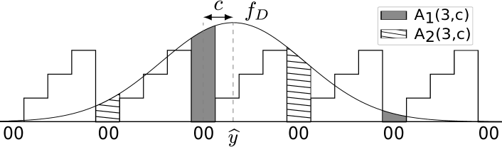
Figure 8: Calculating $L_{3}(\widehat{y})$ by determining the areas $A_{1}(3,c)$ (gray) and $A_{2}(3,c)$ (striped).

Appendix B Proof of Theorem 2

Proof:

The proof is similar to the proof of Thm. 1 and uses $Q_{k-1}(y)$ and $\mathcal{I}_{Q_{k-1}(y)}$, as defined, respectively, in (37) and (38) in Appendix A. When decoding, the quantity $c$ denotes the distance from $\widehat{y}$ to the center of the closest interval consistent with $Q_{k-1}(\widehat{y})$, that is

$$c=\underset{\mathcal{I}\in\mathcal{I}_{Q_{k-1}(\widehat{y})}}{\mathrm{min}}\left|\widehat{y}-\frac{\sup(\mathcal{I})+\inf(\mathcal{I})}{2}\right|.$$ (66)

Fig. 8 illustrates the case where the first $k-1=2$ bits are $00$. The quantity $c$ extends from the predicted measurement $\widehat{y}$ to the center of the closest $00$ quantization interval.

Consider the random variable $D=y-\widehat{y}$, with pdf $f_{D}\left(\cdot\right)$, distributed as $\mathcal{N}(0,\left(\frac{\sigma\epsilon}{\Delta}\right)^{2})$, as shown in Thm. 1. Let $A_{1}(k,c)$ denote the probability that $D$ takes values in the quantization intervals which are consistent with the $k$ bits, $\mathcal{I}_{Q_{k}(\widehat{y})}$, that is

$$A_{1}(k,c)=\int_{t\in\mathcal{T}}f_{D}(t)dt,$$ (67)

where $\mathcal{T}=\bigcup_{\mathcal{I}\in\mathcal{I}_{Q_{k}(\widehat{y})}}\mathcal{I}$. Similarly, let $A_{2}(k,c)$ denote the probability that $D$ takes values in the quantization intervals which are not consistent with $\mathcal{I}_{Q_{k}(\widehat{y})}$. The areas under $f_{D}(\cdot)$ associated with these two probabilities are shown in Fig. 8.

We estimate the likelihood that the $k^{\mathrm{th}}$ bit is flipped as

$$L_{k} =\mathrm{Pr}\left(\widehat{q}_{(k)}\neq q_{(k)}\mid\widehat{y},Q_{k-1}(\widehat{y})\right)$$ (68)

$$=\frac{A_{2}(k,c)}{A_{1}(k,c)+A_{2}(k,c)}.$$ (69)

We use the $2^{k}$-periodic rectangular function of unit width

$$g(t)=\mathrm{rect}(t)\ast\sum_{l=-\infty}^{+\infty}\delta\left(t-l2^{k}\right),$$ (70)

to express (67) as $A_{1}(k,c)=\int_{-\infty}^{+\infty}f_{D}(t)g(t-c)dt$, i.e.,

$$A_{1}(k,c)=\int_{-\infty}^{+\infty}\mathcal{F}\left\{f_{D}(t)\right\}\mathcal{F}\left\{g(t-c)\right\}d\xi$$ (71)

$$=\int\limits_{-\infty}^{+\infty}\!\!\!\!\left(e^{-2\left(\frac{\pi\sigma\epsilon\xi}{\Delta}\right)^{\!2}}\right)\!\!\left(\!e^{-i2\pi\xi c}\mathrm{sinc}(\xi)\frac{1}{2^{k}}\!\!\!\sum_{l=-\infty}^{+\infty}\!\!\!\delta\left(\xi-\frac{l}{2^{k}}\right)\!\right)\!d\xi$$

$$=\frac{1}{2^{k}}\int\limits_{-\infty}^{+\infty}\!e^{-2\left(\frac{\pi\sigma\epsilon\xi}{\Delta}\right)^{2}}\cos(2\pi\xi c)\mathrm{sinc}(\xi)\!\!\sum_{k=-\infty}^{+\infty}\!\!\!\delta\left(\xi-\frac{k}{2^{k}}\right)\!d\xi$$

$$=\frac{1}{2^{k}}\!\Biggl{(}1+2\!\sum_{l=1}^{+\infty}\!e^{-\frac{1}{2}\!\left(\frac{\pi\sigma\epsilon l}{2^{k-1}\Delta}\right)^{\!2}}\!\!\cos\!\left(\!\frac{\pi ck}{2^{k-1}}\!\right)\!\mathrm{sinc}\!\left(\!\frac{l}{2^{k}}\!\right)\!\!\Biggr{)}.$$ (72)

Similarly, we note that inconsistent quantization intervals are shifted by $2^{k-1}$ with respect to consistent intervals, and hence

$$A_{2}(k,c)=A_{1}(k,2^{k-1}-c)$$

$$=\frac{1}{2^{k}}\!\Biggl{(}\!1+2\!\sum_{l=1}^{+\infty}\!e^{-\frac{1}{2}\!\left(\!\frac{\pi\sigma\epsilon l}{2^{k-1}\Delta}\!\right)^{2}}\!\!\!\cos\!\left(\!\!\frac{\pi l\!\left(2^{k-1}-c\right)}{2^{k-1}}\!\!\right)\!\!\mathrm{sinc}\!\left(\!\frac{l}{2^{k}}\!\right)\!\!\Biggr{)}.$$ (73)

∎

Maxim Goukhshtein (GS’16) is currently pursuing a Ph.D. degree in electrical and computer engineering at the University of Toronto, Toronto, ON, Canada. He received the B.Eng. degree in electrical engineering from McGill University, Montreal, QC, Canada in 2015, and the M.A.Sc. degree in electrical and computer engineering from the University of Toronto in 2017. He completed engineering internships at National Instruments, Austin, TX, USA and Ericsson, Ottawa, ON, Canada, and was a Research Intern at the Mitsubishi Electric Research Laboratories (MERL), Cambridge, MA, USA. His research interests lie at the intersection of information theory, coding theory and signal processing. Most recently he has been working on probabilistic shaping and source resolvability. He was previously supported by the Queen Elizabeth II Graduate Scholarship and the Ontario Graduate Scholarship, and currently by the NSERC Postgraduate Scholarship.

Petros T. Boufounos (S’02-M’06-SM’13) is a Senior Principal Research Scientist and the Computational Sensing Team Leader at Mitsubishi Electric Research Laboratories (MERL), and a visiting scholar at the Rice University Electrical and Computer Engineering department. Dr. Boufounos completed his undergraduate and graduate studies at MIT. He received the S.B. degree in Economics in 2000, the S.B. and M.Eng. degrees in Electrical Engineering and Computer Science (EECS) in 2002, and the Sc.D. degree in EECS in 2006. Between September 2006 and December 2008, he was a postdoctoral associate with the Digital Signal Processing Group at Rice University. He joined MERL in January 2009. Dr. Boufounos’ immediate research focus includes signal acquisition and processing, inverse problems, frame theory, quantization and data representations. He is also interested into how signal acquisition interacts with other fields that use sensing extensively, such as machine learning, robotics and dynamical system theory. Dr. Boufounos has served as an Associate Editor and a Senior Area Editor at IEEE Signal Processing Letters, has been part of the SigPort editorial board, and is currently a member of the IEEE Signal Processing Society Theory and Methods technical committee and an Associate Editor at IEEE Transactions on Computational Imaging.

Toshiaki Koike-Akino (M’05–SM’11) received the B.S. degree in electrical and electronics engineering, M.S. and Ph.D. degrees in communications and computer engineering from Kyoto University, Kyoto, Japan, in 2002, 2003, and 2005, respectively. During 2006–2010 he was a Postdoctoral Researcher at Harvard University, and joined MERL, Cambridge, MA, USA, in 2010. His research interests include signal processing for data communications and sensing. He received the YRP Encouragement Award 2005, the 21st TELECOM System Technology Award, the 2008 Ericsson Young Scientist Award, the IEEE GLOBECOM’08 Best Paper Award, the 24th TELECOM System Technology Encouragement Award, and the IEEE GLOBECOM’09 Best Paper Award.

Stark C. Draper (S’99-M’03-SM’15) is a Professor of Electrical and Computer Engineering at the University of Toronto (UofT) and was an Associate Professor at the University of Wisconsin, Madison. As a research scientist he has worked at the Mitsubishi Electric Research Labs (MERL), Disney’s Boston Research Lab, Arraycomm Inc., the C. S. Draper Laboratory, and Ktaadn Inc. He completed postdocs at the University of Toronto and at the University of California, Berkeley. He received the M.S. and Ph.D. degrees from the Massachusetts Institute of Technology (MIT), and the B.S. and B.A. degrees in Electrical Engineering and in History from Stanford University. His research interests include information theory, optimization, error-correction coding, security, and the application of tools and perspectives from these fields in communications, computing, and learning. Prof. Draper has received the NSERC Discovery Award, the NSF CAREER Award, the 2010 MERL President’s Award, and teaching awards from the University of Toronto, the University of Wisconsin, and MIT. He received an Intel Graduate Fellowship, Stanford’s Frederick E. Terman Engineering Scholastic Award, and a U.S. State Department Fulbright Fellowship. He spent the 2019-20 academic year on sabbatical at the Chinese University of Hong Kong, Shenzhen, and visiting the Canada-France-Hawaii Telescope (CFHT) in Hawaii, USA. He chairs the Machine Intelligence major at UofT and serves on the IEEE Information Theory Society Board of Governors.

References

- [1] D. Slepian and J. Wolf, “Noiseless coding of correlated information sources,” IEEE Trans. Inf. Theory, vol. 19, no. 4, pp. 471–480, Sep. 1973.
- [2] A. Wyner and J. Ziv, “The rate-distortion function for source coding with side information at the decoder,” IEEE Trans. Inf. Theory, vol. 22, no. 1, pp. 1–10, Jan 1976.
- [3] D. Schonberg, S. Draper, and K. Ramchandran, “On compression of encrypted images,” in Int. Conf. Image Proc., Oct. 2006, pp. 269–272.
- [4] D. Schonberg, S. C. Draper, C. Yeo, and K. Ramchandran, “Toward compression of encrypted images and video sequences,” IEEE Trans. Inf. Forensics Security, vol. 3, no. 4, pp. 749–762, Dec. 2008.
- [5] B. Girod, A. M. Aaron, S. Rane, and D. Rebollo-Monedero, “Distributed video coding,” Proc. IEEE, vol. 93, no. 1, pp. 71–83, Jan 2005.
- [6] V. Toto-Zarasoa, A. Roumy, and C. Guillemot, “Source modeling for distributed video coding,” IEEE Trans. Circuits Syst. Video Technol., vol. 22, no. 2, pp. 174–187, 2012.
- [7] S. Rane, Y. Wang, P. Boufounos, and A. Vetro, “Wyner-Ziv coding of multispectral images for space and airborne platforms,” in Proc. 28th Picture Coding Symp. (PCS), Nagoya, Japan, Dec. 2010.
- [8] Y. Wang, S. Rane, P. T. Boufounos, and A. Vetro, “Distributed compression of zerotrees of wavelet coefficients,” in Proc. IEEE Int. Conf. Image Proc. (ICIP), Brussels, Belgium, Sep. 2011.
- [9] D. Valsesia and P. T. Boufounos, “Universal encoding of multispectral images,” in Proc. IEEE Int. Conf. Acoust. Speech Sig. Proc. (ICASSP), Shanghai, China, Mar. 2016.
- [10] M. Goukhshtein, P. T. Boufounos, T. Koike-Akino, and S. Draper, “Distributed coding of multispectral images,” in Proc. IEEE Int. Symp. Info. Theory (ISIT), Aachen, Germany, Jun. 2017, pp. 3240–3244.
- [11] T. M. Cover and J. A. Thomas, Elements of Information Theory. New York, NY, USA: Wiley-Interscience, 2006.
- [12] A. El Gamal and Y.-H. Kim, Network Information Theory. Cambridge University Press, 2011.
- [13] A. Wyner, “Recent results in the Shannon theory,” IEEE Trans. Inf. Theory, vol. 20, no. 1, pp. 2–10, Jan 1974.
- [14] T. Ancheta, “Syndrome-source-coding and its universal generalization,” IEEE Trans. Inf. Theory, vol. 22, no. 4, pp. 432–436, Jul 1976.
- [15] S. S. Pradhan and K. Ramchandran, “Distributed source coding using syndromes (DISCUS): design and construction,” IEEE Trans. Inf. Theory, vol. 49, no. 3, pp. 626–643, Mar 2003.
- [16] E. J. Candes and T. Tao, “Decoding by linear programming,” IEEE Trans. Inf. Theory, vol. 51, no. 12, pp. 4203–4215, Dec 2005.
- [17] N. Parikh and S. Boyd, “Proximal algorithms,” Found. Trends Optim., vol. 1, no. 3, pp. 127–239, Jan. 2014.
- [18] M. Friedlander, H. Mansour, R. Saab, and O. Yilmaz, “Recovering compressively sampled signals using partial support information,” IEEE Trans. Inf. Theory, vol. 58, no. 2, pp. 1122–1134, Feb 2012.
- [19] L. Jacques, D. K. Hammond, and J. M. Fadili, “Dequantizing compressed sensing: When oversampling and non-Gaussian constraints combine,” IEEE Trans. Info. Theory, vol. 57, no. 1, pp. 559–571, Jan 2011.
- [20] W. Dai, H. V. Pham, and O. Milenkovic, “Distortion-rate functions for quantized compressive sensing,” in Proc. IEEE Info. Theory Workshop on Netw. and Info. Theory, Volos, Greece, Jun. 2009, pp. 171–175.
- [21] P. T. Boufounos, L. Jacques, F. Krahmer, and R. Saab, “Quantization and compressive sensing,” in Compressed sensing and its applications. Springer, 2015, pp. 193–237.
- [22] J. Z. Sun and V. K. Goyal, “Optimal quantization of random measurements in compressed sensing,” in Proc. IEEE Int. Symp. on Info. Theory (ISIT), Seoul, South Korea, June 2009, pp. 6–10.
- [23] A. Kipnis, G. Reeves, Y. C. Eldar, and A. J. Goldsmith, “Compressed sensing under optimal quantization,” in Proc. IEEE Int. Symp. on Info. Theory (ISIT), Aachen, Germany, June 2017, pp. 2148–2152.
- [24] P. Boufounos and R. Baraniuk, “Quantization of sparse representations,” in Proc. Data Compression Conf., Snowbird, UT, USA, Mar. 2007, pp. 378–378.
- [25] A. Zymnis, S. Boyd, and E. Candes, “Compressed sensing with quantized measurements,” IEEE Signal Proc. Lett., vol. 17, no. 2, pp. 149–152, Feb 2010.
- [26] W. Dai, H. V. Pham, and O. Milenkovic, “A comparative study of quantized compressive sensing schemes,” in Proc. IEEE Int. Symp. on Info. Theory (ISIT), Seoul, South Korea, June 2009, pp. 11–15.
- [27] U. Kamilov, “Optimal quantization for sparse reconstruction with relaxed belief propagation,” Master’s thesis, EPFL/MIT, 2001.
- [28] L. Jacques, K. Degraux, and C. De Vleeschouwer, “Quantized iterative hard thresholding: Bridging 1bit and high-resolution quantized compressed sensing,” in Proc. 10th Int. Conf. Sampling Theory Appl. (SampTA), Bremen, Germany, Jul. 2013, pp. 105–108.
- [29] J. N. Laska, P. T. Boufounos, M. A. Davenport, and R. G. Baraniuk, “Democracy in action: Quantization, saturation, and compressive sensing,” Applied and Computational Harmonic Analysis, vol. 31, no. 3, pp. 429–443, Nov. 2011.
- [30] R. G. Baraniuk, V. Cevher, M. F. Duarte, and C. Hegde, “Model-based compressive sensing,” IEEE Trans. Inf. Theory, vol. 56, no. 4, pp. 1982–2001, 2010.
- [31] A. Gersho and R. M. Gray, Vector Quantization and Signal Compression. USA: Kluwer Academic Publishers, 1991.
- [32] D. Baron, M. F. Duarte, M. B. Wakin, S. Sarvotham, and R. G. Baraniuk, “Distributed compressive sensing,” 2009, arXiv:0901.3403.
- [33] M. F. Duarte, M. B. Wakin, D. Baron, S. Sarvotham, and R. G. Baraniuk, “Measurement bounds for sparse signal ensembles via graphical models,” IEEE Trans. Inf. Theory, vol. 59, no. 7, pp. 4280–4289, 2013.
- [34] L. Kang and C. Lu, “Distributed compressive video sensing,” in Proc. IEEE Int. Conf. Acoust. Speech Sig. Proc. (ICASSP), Taipei, Taiwan, Apr. 2009, pp. 1169–1172.
- [35] H. Liu, Y. Li, S. Xiao, and C. Wu, “Distributed compressive hyperspectral image sensing,” in Proc. Sixth Int. Conf on Intelligent Information Hiding and Multimedia Sig. Proc. (IIH-MSP), Darmstadt, Germany, Oct. 2010, pp. 607–610.
- [36] A. Shirazinia, S. Chatterjee, and M. Skoglund, “Distributed quantization for compressed sensing,” in Proc. IEEE Int. Conf. Acoust. Speech Sig. Proc. (ICASSP), Florence, Italy, May 2014, pp. 6439–6443.
- [37] A. Shirazinia, S. Chatterjee, and M. Skoglund, “Distributed quantization for measurement of correlated sparse sources over noisy channels,” 2014, arXiv:1404.7640.
- [38] P. Boufounos, “Universal rate-efficient scalar quantization,” IEEE Trans. Inf. Theory, vol. 58, no. 3, pp. 1861–1872, Mar. 2012.
- [39] P. T. Boufounos, “Hierarchical distributed scalar quantization,” in Proc. 9th Int. Conf. Sampling Theory Appl. (SampTA), Singapore, May 2011.
- [40] D. Valsesia and P. T. Boufounos, “Multispectral image compression using universal vector quantization,” in Proc. IEEE Inf. Theory Workshop (ITW), Cambridge, UK, Sept. 2016.
- [41] G. Coluccia, E. Magli, A. Roumy, and V. Toto-Zarasoa, “Lossy compression of distributed sparse sources: A practical scheme,” in Proc. 19th European Sig. Proc. Conf., Barcelona, Spain, Aug.-Sep. 2011.
- [42] G. Coluccia, C. Ravazzi, and E. Magli, Compressed sensing for distributed systems. Springer, 2015.
- [43] A. Elzanaty, A. Giorgetti, and M. Chiani, “Lossy compression of noisy sparse sources based on syndrome encoding,” IEEE Trans. Commun., vol. 67, no. 10, pp. 7073–7087, 2019.
- [44] A. Eftekhari and M. B. Wakin, “New analysis of manifold embeddings and signal recovery from compressive measurements,” Applied and Computational Harmonic Analysis, vol. 39, no. 1, pp. 67 – 109, 2015.
- [45] D. Van Veen, A. Jalal, M. Soltanolkotabi, E. Price, S. Vishwanath, and A. G. Dimakis, “Compressed sensing with deep image prior and learned regularization,” 2018, arXiv:1806.06438.
- [46] L. Schuchman, “Dither signals and their effect on quantization noise,” IEEE Trans. Commun. Technol., vol. 12, no. 4, pp. 162–165, Dec. 1964.
- [47] H. Imai and S. Hirakawa, “A new multilevel coding method using error-correcting codes,” IEEE Trans. Inf. Theory, vol. 23, no. 3, pp. 371–377, May 1977.
- [48] N. Ailon and H. Rauhut, “Fast and RIP-optimal transforms,” Discrete Comput. Geom., vol. 52, no. 4, pp. 780–798, Dec. 2014.
- [49] M. F. Duarte, M. A. Davenport, D. Takhar, J. N. Laska, T. Sun, K. F. Kelly, and R. G. Baraniuk, “Single-pixel imaging via compressive sampling,” IEEE Sig. Proc. Mag., vol. 25, no. 2, pp. 83–91, Mar. 2008.
- [50] J. A. Tropp, “Improved analysis of the subsamples randomized Hadamard transform,” Adv. Adaptive Data Analysis, vol. 03, 11 2010.
- [51] J. Chen, D. . He, and A. Jagmohan, “The equivalence between slepian-wolf coding and channel coding under density evolution,” IEEE Trans. Commun, vol. 57, no. 9, pp. 2534–2540, 2009.
- [52] J. Chen, D. He, and A. Jagmohan, “On the duality between slepian–wolf coding and channel coding under mismatched decoding,” IEEE Trans. Inf. Theory, vol. 55, no. 9, pp. 4006–4018, 2009.
- [53] A. Abrardo, M. Barni, E. Magli, and F. Nencini, “Error-resilient and low-complexity onboard lossless compression of hyperspectral images by means of distributed source coding,” IEEE Trans. Geosci. Remote Sens., vol. 48, no. 4, pp. 1892–1904, Apr. 2010.
- [54] D. Valsesia and E. Magli, “A novel rate control algorithm for onboard predictive coding of multispectral and hyperspectral images,” IEEE Trans. Geosci. Remote Sens., vol. 52, no. 10, pp. 6341–6355, Oct. 2014.
- [55] J. N. Laska and R. G. Baraniuk, “Regime change: Bit-depth versus measurement-rate in compressive sensing,” IEEE Trans. Sig. Proc., vol. 60, no. 7, pp. 3496–3505, July 2012.
- [56] Y. Polyanskiy, H. V. Poor, and S. Verdu, “Channel coding rate in the finite blocklength regime,” IEEE Trans. Inf. Theory, vol. 56, no. 5, pp. 2307–2359, 2010.
- [57] V. Y. F. Tan, “Asymptotic estimates in information theory with non-vanishing error probabilities,” Foundations and Trends® in Communications and Information Theory, vol. 11, no. 1-2, pp. 1–184, 2014.
- [58] U. Kamilov, “A parallel proximal algorithm for anisotropic total variation minimization,” IEEE Trans. Image Proc., vol. 26, no. 2, pp. 539–548, 2017.
- [59] Japan Aerospace Exploration Agency Earth Observation Research Center. “About ALOS - AVNIR-2”. [Online]. Available: http://www.eorc.jaxa.jp/ALOS/en/about/avnir2.htm
- [60] A. Bora, A. Jalal, E. Price, and A. G. Dimakis, “Compressed sensing using generative models,” in Proc. 34th Int. Conf. Machine Learning (ICML), Sydney, NSW, Australia, 2017, pp. 537–546.