A Query-Efficient Quantum Algorithm for Maximum Matching on General Graphs

Abstract

We design quantum algorithms for maximum matching. Working in the query model, in both adjacency matrix and adjacency list settings, we improve on the best known algorithms for general graphs, matching previously obtained results for bipartite graphs. In particular, for a graph with $n$ vertices and $m$ edges, our algorithm makes $O(n^{7/4})$ queries in the matrix model and $O(n^{3/4}(m+n)^{1/2})$ queries in the list model. Our approach combines Gabow’s classical maximum matching algorithm [Gabow, Fundamenta Informaticae, ’17] with the guessing tree method of Beigi and Taghavi [Beigi and Taghavi, Quantum, ’20].

1 Introduction

A matching is a set of non-adjacent edges in an undirected graph. In the maximum matching problem, one tries to find the matching with the largest number of edges. Finding the maximum matching in a graph is a problem that is both of fundamental and practical importance. Its practical applications range from kidney exchange to scheduling to characterizing chemical structures [17, 7, 14]. As a fundamental problem, it has stimulated a string of algorithmic developments, such as the use of blossoms and dual variables [6], which have been useful in the development of a broad range of algorithms. Additionally, maximum matching in general (bipartite and non-bipartite) graphs is notable for the difficulty researchers have had in finding a simple and correct algorithm for this seemingly straightforward problem [15, 8].

We study maximum matching in the query setting: We are given a graph $G$ as an adjacency matrix or adjacency list and the goal is to find a maximum matching with as few queries as possible. A query in the matrix model takes the form, “Do vertices $\operatorname*{\mathnormal{x}}$ and $\operatorname*{\mathnormal{y}}$ share an edge?” A query in the list model takes the form, “What is the $i$th vertex adjacent to vertex $\operatorname*{\mathnormal{x}}$?”

The best classical algorithms for maximum matching solve the problem in $O(m\sqrt{n})$ time for both bipartite and general graphs [8, 9, 15, 18]. The query complexity of these classical algorithms is the trivial $O(n^{2})$ in the matrix model and $O(m)$ in the list model. In fact, using an adversarial argument, it is easy to see that any classical algorithm must query all pairs of vertices or all edges to find a maximum matching in the worst case.

Using quantum computers, however, we can do better. Lin and Lin found a quantum algorithm that solves maximum matching on a bipartite graph in $O(n^{7/4})$ queries in the matrix model [13]. Beigi and Taghavi created an algorithm that uses $O(n^{3/4}\sqrt{m+n})$ queries in the list model for bipartite graphs [3], which in the worst case when $m=\Omega(n^{2})$, matches the result of Lin and Lin. Both results use the guessing tree method: Lin and Lin introduced the method for functions with binary input and Beigi and Taghavi generalized it to functions with non-binary input.

Our contribution is a quantum maximum matching algorithm for general graphs that uses $O(n^{7/4})$ queries in the matrix model and $O(n^{3/4}\sqrt{m+n})$ in the list model, matching the prior results for bipartite graphs. We combine two powerful techniques to obtain our result: Beigi and Taghavi’s guessing tree method and Gabow’s relatively simple algorithm for maximum matching [3, 8]. The key technical issues in combining these two approaches are a careful accounting of which steps of the classical algorithm actually require queries, slight modifications to the classical algorithm that help us bound the number of queries, and a well-chosen definition of the guessing scheme for the decision tree used in the guessing tree method.

The previous best known quantum algorithms for maximum matching on general graphs ran in trivial query complexity. Ambainis and Špalek designed algorithms for general maximum matching that run in $O(n^{5/2}\log n)$ time in the matrix model and $O(n^{2}(\sqrt{m/n}+\log n)\log n)$ time in the list model [2]. Dörn found an algorithm for general maximum matching that runs in $O(n^{2}\log^{2}n)$ time in the matrix model and $O(n\sqrt{m}\log^{2}n)$ time in the list model [5].

While our result unifies the cases of bipartite and general graphs, there remains a gap between our upper bound and the best known lower bound. Berzina et al. and Zhang found a lower bound for maximum matching of $O(n^{3/2})$ [4, 19]. Interestingly, Zhang proved that Ambainis techniques (one of the most useful methods for finding quantum lower bounds) cannot improve the current lower bound [1, 19].

1.1 Graph Theory

Given an undirected graph $G$, we denote by $V(G)$ the set of vertices and $E(G)$ be the set of edges of $G$. Call $n=|V(G)|$ the number of vertices in a graph and $m=|E(G)|$ the number of edges. We represent an edge between vertices $\operatorname*{\mathnormal{x}}$ and $\operatorname*{\mathnormal{y}}$ as $\operatorname*{\mathnormal{xy}}$.

We denote the symmetric difference of two graphs $G_{1}$ and $G_{2}$ as $G_{1}\oplus G_{2}$. Then $V(G_{1}\oplus G_{2})$ is $V(G_{1})\cup V(G_{2})$ and $\operatorname*{\mathnormal{xy}}\in E(G_{1}\oplus G_{2})$ if and only if $\operatorname*{\mathnormal{xy}}\in E(G_{1})$ but $\operatorname*{\mathnormal{xy}}\notin E(G_{2})$ or $\operatorname*{\mathnormal{xy}}\in E(G_{2})$ but $\operatorname*{\mathnormal{xy}}\notin E(G_{1})$. We may think of the symmetric difference as the graph equivalent of addition modulo 2.

A matching $M$ is a set of non-adjacent edges of $G$. That is, if $\operatorname*{\mathnormal{xy}}$ is in $M$, then there is no other edge connected to $\operatorname*{\mathnormal{x}}$ or $\operatorname*{\mathnormal{y}}$ in $M$. The solid edges in Figure 1 form a matching. A maximum matching on $G$ is a matching with the most edges of any matching on $G$. We call a vertex a free vertex if it is not on any edge in matching $M$, while if a vertex is not free we called it matched. A matched edge is in a matching while an unmatched edge is not.

A blossom is a cycle of length $2k+1$ with $k$ matched edges and $k+1$ unmatched edges. The edges alternate between matched and unmatched edges with the exception of the two edges connected to the root of the blossom. In Figure 1, the blossom has $2(2)+1=5$ edges and the root is the vertex in the cycle closest to the left free vertex.

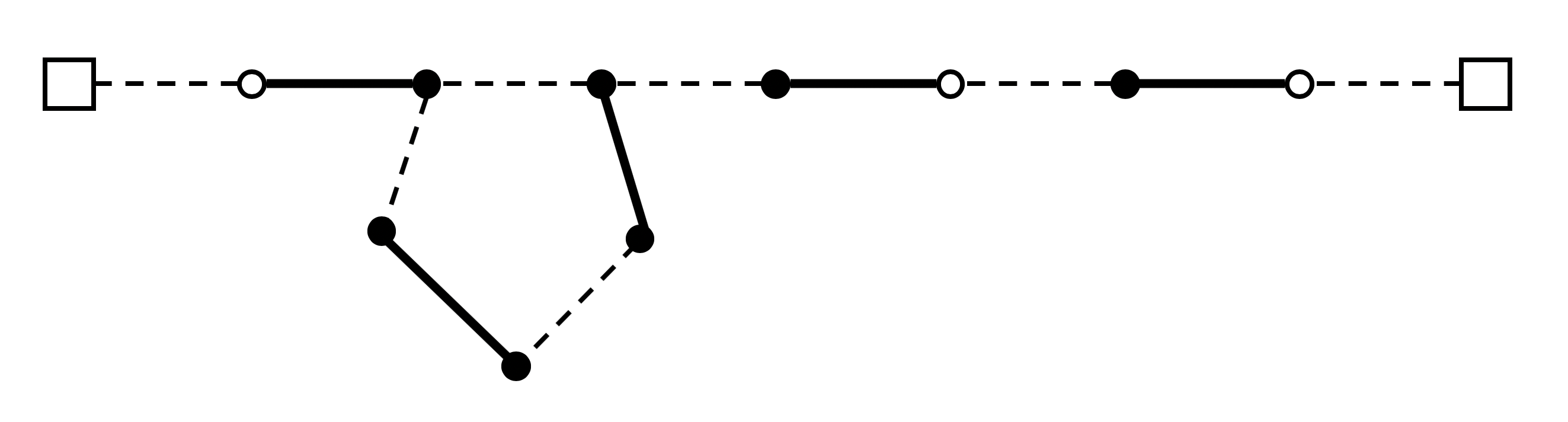
Figure 1: Example graph with a matching where the solid lines are edges in the matching and the dotted lines are edges not in the matching but in the underlying graph. The free vertices are squares, the outer vertices (excluding the free vertices) are filled circles, and the inner vertices are hollow circles.

An augmenting path is a set of edges between two free vertices that alternates between matched and unmatched edges. In Figure 1, the horizontal edges connecting the two free vertices (represented as squares) is not an augmenting path because there are two consecutive unmatched edges. A sap (shortest augmenting path) is an augmenting path with the fewest edges of any augmenting path. In Figure 1, the augmenting path along the blossom between the free vertices forms a sap. We call a vertex inner with respect to an augmenting path if it is closer than its matched pair (the vertex with which it shares a matched edge) to the closest free vertex. Here ‘closeness’ is measured by the number of edges on the augmenting path between the vertex in question and the closest free vertex. Inner vertices are illustrated in Figure 1 as hollow circles. All other vertices—including free vertices, all vertices on a blossom, and vertices adjacent to an edge equidistant between two free vertices—are outer. Whether a vertex is inner or outer may change as the augmenting paths grow: An inner vertex can become outer (e.g. if it becomes part of a blossom) but an outer vertex cannot become inner.

Notice that we can use the partial matching and sap in Figure 1 to get a larger (in this case maximum) matching. We simply take the symmetric difference of the partial matching and augmenting path. That is, we include every unmatched edge (since it is in augmenting path but not the partial matching) and remove every matched edge (since it is in both the augmenting path and the partial matching). The result is a larger matching where each vertex with an edge in the partial matching has an edge in the larger matching and the previously free vertices also have matched edges.

1.2 Query Complexity

In both the list and matrix models, we learn the edges of $G$ by querying (i.e. evaluating at various inputs) a function. We assume that $G$ is a subgraph of the complete graph of $n$ vertices, labeled by elements of $[n]=\{0,1,\dots,n-1\}$, where we do not know which edges of the complete graph are part of $G$ and which are not. Then in the case of the adjacency matrix, we have a function $E_{M}:[n]\times[n]\rightarrow\{0,1\}$, where $E_{M}(\operatorname*{\mathnormal{x}},\operatorname*{\mathnormal{y}})=1$ if and only if the edge $\operatorname*{\mathnormal{xy}}\in E(G)$.

In the case of the adjacency list, we have a function $E_{L}:[n]\times[n]\rightarrow[n]\cup\{\texttt{null}\}$ where

$$E_{L}(\operatorname*{\mathnormal{x}},i)=\begin{cases}\operatorname*{\mathnormal{y}}&\textrm{ if $\operatorname*{\mathnormal{y}}$ is the }i\textrm{th neighbor of }\operatorname*{\mathnormal{x}}\\ \texttt{null}&\textrm{ if u has less than }i\textrm{ neighbors}\end{cases}.$$

Given access to one of these functions, the classical bounded error query complexity of maximum matching is the number of times we must evaluate the function in order to find a maximum matching with high probability.

In the quantum model, we are given access to unitaries called oracles that encode the information of the functions $E_{M}$ and $E_{L}$. In the adjacency matrix model, we have access to an oracle $O_{M}$ that acts on the Hilbert space $\mathbb{C}^{n}\times\mathbb{C}^{n}\times\mathbb{C}^{2}$ such that for an edge $e=\operatorname*{\mathnormal{xy}}$, and $b\in\{0,1\}$, $O_{M}|e\rangle|b\rangle=|e\rangle|b\oplus E_{M}(e)\rangle$, where addition is modulo 2. In the adjacency list model, we have access to an oracle $O_{L}$ that acts on the Hilbert space $\mathbb{C}^{n}\times\mathbb{C}^{n}\times\mathbb{C}^{n+1}$, where for a vertex $\operatorname*{\mathnormal{x}}$, index $i$, and $j\in[n+1]$, acts as $O_{L}|\operatorname*{\mathnormal{x}},i\rangle|j\rangle=|\operatorname*{\mathnormal{x}},i\rangle|j\oplus E_{L}(\operatorname*{\mathnormal{x}},i)\rangle$, where addition is modulo $n+1.$

Given access to one of these oracles, the quantum bounded error query complexity of maximum matching is the number of times we must apply the oracle (as part of a quantum algorithm) in order to find a maximum matching with high probability.

Given a classical query algorithm, one can create a decision tree that describes the sequence and outcomes of queries that are made throughout the algorithm. Each non-leaf vertex in the tree represents a query, and the outgoing edges from a vertex represent possible outcomes of the query. Sets of query outcomes may be grouped into a single edge (provided future decisions made by the algorithm are independent of which particular query outcome within the set occurred). Given such a decision tree, one can create a guessing scheme. A guessing scheme is a labeling of edges such that exactly one outgoing edge from each vertex is labelled as the guess. If the outcome of a query matches the guess, we say that the guessing scheme correctly guessed the outcome of that query. Otherwise, we say it was an incorrect guess.

Given such a decision tree and guessing algorithm, it is possible to design a quantum algorithm:

Theorem 1.1 (Guessing Tree [3])

For positive integers $k$, $\ell$, and $m$, let $f:D_{f}\rightarrow[k]$ be a function with $D_{f}\subseteq[\ell]^{m}$. Let $\mathcal{T}$ be a decision tree for $f$ with a guessing scheme and let $T$ be the depth of $\mathcal{T}$. Define $I$ as the maximum number of incorrect guesses in any path from the root to a leaf of $\mathcal{T}$. Then the bounded error quantum query complexity of evaluating $f$ is upper bounded by $O(\sqrt{TI})$. The quantum space complexity is $O(m)$.

See Beigi and Taghavi [3] for extensive applications of Theorem 1.1. Observe that the size of the image of the function $f$ does not affect the query complexity or space complexity of the quantum algorithm that evaluates it. We use this fact to specify the maximum matching (all $O(n)$ edges) in the leaves of our decision tree.

2 Result

We use Gabow’s algorithm to find a maximum matching in graph $G$. Gabow’s algorithm runs in two phases. (The high level pseudocode is in LABEL:list:overview.) In the first phase, the algorithm finds all the edges in $G$ that are on saps. In the second phase, the algorithm finds disjoint saps that are used to augment the partial matching. Since a maximal set of disjoint saps are found in each iteration, there are at most $O(\sqrt{n})$ iterations [9].

Listing 2.1: Gabow’s Algorithm [8]

⬇

1$M\leftarrow\emptyset$ /* M is the current partial matching */

2loop

3 /* Phase 1 */

4 for every pair of vertices $\operatorname*{\mathnormal{x}},\operatorname*{\mathnormal{y}}$ do

5 if $\operatorname*{\mathnormal{xy}}\in M$ then $w(\operatorname*{\mathnormal{x}},\operatorname*{\mathnormal{y}})\leftarrow 2$ else $w(\operatorname*{\mathnormal{x}},\operatorname*{\mathnormal{y}})\leftarrow 0$

6 Listing 2/3 (matrix/list model) to find pairs of vertices on saps

7 if no augmenting path is found then

8 break /* $M$ has maximum cardinality */

9

10 /* Phase 2 */

11 Listing 4/5 (matrix/list) to create maximal set of disjoint saps $P$

12 augment $M$ by the paths of $P$

The key idea behind the algorithm is the use of dual variables associated with each vertex, and which we denote using a function $d:V\rightarrow\mathbb{Z}$. Each dual variable is initialized to 1. A pair of vertices is tight if the sum of the dual variables $d(\operatorname*{\mathnormal{x}})$ and $d(\operatorname*{\mathnormal{y}})$ is $w(\operatorname*{\mathnormal{x}},\operatorname*{\mathnormal{y}})$. Recall from LABEL:list:overview that $w(\operatorname*{\mathnormal{x}},\operatorname*{\mathnormal{y}})$ is 2 if $\operatorname*{\mathnormal{xy}}$ is a matched edge and 0 otherwise. Intuitively, a pair of vertices is tight only if their shared edge could be part of a sap [8].

We use Gabow’s maximum matching algorithm to construct a decision tree that finds a maximum matching. To apply Theorem 1.1 to the decision tree, we must design a guessing scheme. In the matrix model, we always guess that the edge we are querying is not present.

In the list model, when we are querying the $i^{th}$ vertex adjacent to $\operatorname*{\mathnormal{x}}$ (call it $\operatorname*{\mathnormal{y}}$), our guess depends on the phase of the algorithm. In the first phase, we guess that $\operatorname*{\mathnormal{x}}$ and $\operatorname*{\mathnormal{y}}$ do not fit either of the following criteria:

• $\operatorname*{\mathnormal{x}}$ and $\operatorname*{\mathnormal{y}}$ are tight, $\operatorname*{\mathnormal{x}}$ and $\operatorname*{\mathnormal{y}}$ are not from the same blossom, and $\operatorname*{\mathnormal{y}}$ has not yet been found (i.e. added to $S$, see LABEL:list:bfs_list), or

• $\operatorname*{\mathnormal{x}}$ and $\operatorname*{\mathnormal{y}}$ are tight, $\operatorname*{\mathnormal{x}}$ and $\operatorname*{\mathnormal{y}}$ are not from the same blossom, and $\operatorname*{\mathnormal{y}}$ is outer.

In the second phase, we guess that $\operatorname*{\mathnormal{x}}$ and $\operatorname*{\mathnormal{y}}$ do not fit either of the following criteria:

• $\operatorname*{\mathnormal{x}}$ and $\operatorname*{\mathnormal{y}}$ are tight, $\operatorname*{\mathnormal{x}}$ and $\operatorname*{\mathnormal{y}}$ do not share a matched edge, and $\operatorname*{\mathnormal{y}}$ has not yet been found (i.e. added to $S^{\prime}$, see LABEL:list:dfs_list), or

• $\operatorname*{\mathnormal{x}}$ and $\operatorname*{\mathnormal{y}}$ are tight, $\operatorname*{\mathnormal{x}}$ and $\operatorname*{\mathnormal{y}}$ do not share a matched edge, and $\operatorname*{\mathnormal{x}}$ and $\operatorname*{\mathnormal{y}}$ form a blossom.

If our query to the list returns null, that is, we have reached the end of a vertex’s adjacency list, we say that our guess is incorrect.

In the list model, while there might be multiple outcomes of a single query that satisfy the correct guess conditions, we will see that the subsequent behavior of the algorithm is the same, so we group all such correct outcomes into a single edge in our decision tree, as described in Section 1.2.

Applying the above guessing scheme to Gabow’s algorithm, we prove our main result:

Theorem 2.1

Given a graph $G$ with $m$ edges and $n$ vertices, there is a bounded error quantum algorithm that finds a maximum matching in $O(n^{7/4})$ queries in the matrix model and $O(n^{3/4}\sqrt{m+n})$ queries in the list model.

In the remainder of this section, we explain enough of Gabow’s algorithm to analyze the performance of the quantum algorithm and to prove Theorem 2.1. However, we do not address the correctness of Gabow’s algorithm or provide sufficient details to understand why the algorithm is correct. Instead, we encourage interested readers to peruse Gabow’s paper [8].

The choice to not make this paper self-contained is intentional: including the full details of Gabow’s algorithm would double the length of this work without adding any novel contributions.

2.1 Breadth-First Search Subroutine

The first phase of Gabow’s algorithm is a simplified search based on Edmonds’ algorithm that explores $G$ breadth-first [6]. The goal is to identify all the edges that are on saps. For this purpose, the algorithm maintains a subgraph $S$ of $G$ with the vertices and edges that have been explored. Initially, $S$ consists of only free vertices. As the algorithm progresses, edges and vertices are added. We call the set of edges and vertices connected to a free vertex a search tree. The algorithm terminates once two search trees become connected i.e. there is an augmenting path from one free vertex to another.

The algorithm also maintains a record of the blossom that contains $\operatorname*{\mathnormal{x}}$, denoted by $B_{\operatorname*{\mathnormal{x}}}$. We initially set $B_{\operatorname*{\mathnormal{x}}}=\operatorname*{\mathnormal{x}}$ since every vertex is a trivial blossom and redefine $B_{\operatorname*{\mathnormal{x}}}$ when merging blossoms. When all tight pairs of vertices have been checked and no sap has been found, the dual variables are adjusted to find new tight pairs of vertices. If the dual variables cannot be adjusted, there are no augmenting paths and the partial matching is maximum.

The execution of the simplified search based on Edmonds’ algorithm depends on the data structure of the input graph. In the case of the matrix model described in LABEL:list:bfs_matrix, we first identify vertices $\operatorname*{\mathnormal{x}}$ and $\operatorname*{\mathnormal{y}}$ that fit the criteria on Line 4. We then query the edge $\operatorname*{\mathnormal{xy}}$ only if $\operatorname*{\mathnormal{x}}$ and $\operatorname*{\mathnormal{y}}$ satisfy either the if-statement on Line 5 or the if-statement on Line 8. If we reach neither Line 6 nor Line 9 then no query is made in that iteration. If we make a query on Line 6 or Line 9 and the edge is not present, our guess is correct. In order to bound the number of incorrect guesses, we bound the number of times we reach Line 7 and Line 10 which happens only if $\operatorname*{\mathnormal{xy}}$ is present and is in the grow, blossom, or sap case.

Listing 2.2: Simplified Search based on Edmonds’ Algorithm in the Matrix Model [8]

⬇

1for every vertex $\operatorname*{\mathnormal{x}}$ do $d(\operatorname*{\mathnormal{x}})\leftarrow 1$

2make every free vertex outer and add to $V(S)$

3loop

4 if $\exists$ tight pair $\operatorname*{\mathnormal{x}},\operatorname*{\mathnormal{y}}$ with $\operatorname*{\mathnormal{x}}$ outer, $B_{\operatorname*{\mathnormal{x}}}\neq B_{\operatorname*{\mathnormal{y}}}$ then

5 if $\operatorname*{\mathnormal{y}}\notin V(S)$ then /* grow step */

6 if $\operatorname*{\mathnormal{xy}}\in E(G)$ /* query */ then

7 add $\operatorname*{\mathnormal{x}}\operatorname*{\mathnormal{y}},\operatorname*{\mathnormal{y}}\operatorname*{\mathnormal{y}}^{\prime}$ to $S$ where $\operatorname*{\mathnormal{y}}\operatorname*{\mathnormal{y}}^{\prime}\in M$

8 else if $\operatorname*{\mathnormal{y}}$ is outer then

9 if $\operatorname*{\mathnormal{xy}}\in E(G)$ /* query */ then

10 if $\operatorname*{\mathnormal{x}}$ and $\operatorname*{\mathnormal{y}}$ in the same search tree then

11 /* blossom step */

12 merge all blossoms in fundamental cycle of $\operatorname*{\mathnormal{xy}}$

13 else /* $\operatorname*{\mathnormal{xy}}$ forms a sap */

14 return /* continue in Listing 1 */

15 else

16 dual adjustment step

17 /* no queries are made, see Gabow Figure 2 for details */

In the case of the list model described in LABEL:list:bfs_list, we query from an outer vertex $\operatorname*{\mathnormal{x}}$ and find some adjacent vertex $\operatorname*{\mathnormal{y}}$. If $\operatorname*{\mathnormal{x}}$ and $\operatorname*{\mathnormal{y}}$ are not tight, $\operatorname*{\mathnormal{x}}$ and $\operatorname*{\mathnormal{y}}$ are not from the same blossom or neither of the criteria on Lines 9 and 11 apply, then our guess is correct. We bound the number of incorrect guesses by the number of times we reach Lines 7, 10, and 12, which happens only if we have reached the end of $\operatorname*{\mathnormal{x}}$’s neighbors or $\operatorname*{\mathnormal{x}}$ and $\operatorname*{\mathnormal{y}}$ are in the grow, blossom, or sap case.

Observe that we can group the correct guesses in the list model into a single edge in the decision tree because the algorithm’s behavior is the same in every case: continue to query neighbors of $\operatorname*{\mathnormal{x}}$.

Lemma 1

The simplified search of Edmonds’ algorithm makes at most $O(n)$ incorrect guesses in a single call.

Proof

As discussed above, in both the matrix and list models, a guess is incorrect only if we are in the grow, blossom, or sap case (or in the list model at the end of a list). Therefore we bound the number of incorrect guesses by the number of times we can reach each case. In the grow case where $\operatorname*{\mathnormal{y}}\notin S$, we add both $\operatorname*{\mathnormal{y}}$ and $\operatorname*{\mathnormal{y}}^{\prime}$ to $S$, where $\operatorname*{\mathnormal{y}}\operatorname*{\mathnormal{y}}^{\prime}$ is in the current partial matching $M$. Since this case only occurs when a vertex $\operatorname*{\mathnormal{y}}$ is not in $S$, and there are at most $n$ vertices in the graph, this case can trigger at most $n$ incorrect guesses.

In the blossom case where $\operatorname*{\mathnormal{x}}$ and $\operatorname*{\mathnormal{y}}$ are in the same search tree, we have merged at least two blossoms. Each vertex is initially a blossom so we start with a total of $n$ blossoms. Each time we merge two or more blossoms, we reduce the number of blossoms by at least one. Therefore we can merge blossoms at most $n$ times, and so we can only make $n$ incorrect guesses in this case.

In the case where $\operatorname*{\mathnormal{xy}}$ completes a sap, we halt the algorithm and so this may happen at most once per call. In the list model, we can reach the end of a list at most $n$ times so the number of incorrect guesses due to null outcomes is bounded by $n$.

Listing 2.3: Simplified Search based on Edmonds’ Algorithm in the List Model

⬇

1for every vertex $\operatorname*{\mathnormal{x}}$ do $d(\operatorname*{\mathnormal{x}})\leftarrow 1$

2make every free vertex outer and add to $V(S)$

3loop

4 for every outer vertex $\operatorname*{\mathnormal{x}}$ do

5 for every vertex $\operatorname*{\mathnormal{y}}$ adjacent to $\operatorname*{\mathnormal{x}}$ do

6 if $\operatorname*{\mathnormal{y}}$ is null then /* end of list */

7 break /* go to next $\operatorname*{\mathnormal{x}}$ */

8 else if $\operatorname*{\mathnormal{x}}$ and $\operatorname*{\mathnormal{y}}$ are tight and $B_{\operatorname*{\mathnormal{x}}}\neq B_{\operatorname*{\mathnormal{y}}}$ then

9 if $\operatorname*{\mathnormal{y}}\notin V(S)$ then /* grow step */

10 add $\operatorname*{\mathnormal{x}}\operatorname*{\mathnormal{y}},\operatorname*{\mathnormal{y}}\operatorname*{\mathnormal{y}}^{\prime}$ to $S$ where $\operatorname*{\mathnormal{y}}\operatorname*{\mathnormal{y}}^{\prime}\in M$

11 else if $\operatorname*{\mathnormal{y}}$ is outer then

12 if $\operatorname*{\mathnormal{x}}$ and $\operatorname*{\mathnormal{y}}$ in the same search tree then

13 /* blossom step */

14 merge all blossoms in fundamental cycle of $\operatorname*{\mathnormal{xy}}$

15 else /* $\operatorname*{\mathnormal{xy}}$ forms a sap */

16 return /* continue in Listing 1 */

17 dual adjustment step

18 /* no queries are made, see Gabow Fig. 2 for details */

2.2 Depth-First Search Subroutine

In the second phase of the algorithm—the path-preserving depth-first search—we identify disjoint saps. We define a subgraph $H$ of the complete graph which we initialize with the edges between every pair of tight vertices in $S$. (While many edges in $H$ were queried in the breadth-first subroutine, not all were; in particular, most edges between search trees have not yet been queried.) The algorithm explores $H$ from each free vertex in order to find another free vertex.

Listing 2.4: Path-Preserving Depth-First Search in the Matrix Model [8]

⬇

1initialize $P$ to an empty set

2for each free vertex $f$ do

3 if $f\notin V(P)$ then

4 initialize $S^{\prime}$ to an empty graph

5 add $f$ to $S^{\prime}$ as the root of a new search tree

6 $find\_ap(f)$

7

8procedure $find\_ap(\operatorname*{\mathnormal{x}}:$ /* $\operatorname*{\mathnormal{x}}$ is an outer vertex */

9 for each edge $\operatorname*{\mathnormal{xy}}\in E(H)\setminus M$ do

10 if $\operatorname*{\mathnormal{y}}\notin V(S^{\prime})$ then

11 if $\operatorname*{\mathnormal{xy}}\in E(G)$ /* query */ then

12 if $\operatorname*{\mathnormal{y}}$ is free then /* $\operatorname*{\mathnormal{y}}$ completes a sap */

13 add $\operatorname*{\mathnormal{xy}}$ to $S^{\prime}$ and sap to $P$

14 terminate all current recursive calls to $find\_ap$

15 remove all edges of sap from $H$

16 recursively remove all dangling edges from $H$

17 else /* grow step */

18 add $\operatorname*{\mathnormal{xy}},\operatorname*{\mathnormal{y}}\operatorname*{\mathnormal{y}}^{\prime}$ to $S^{\prime}$ where $\operatorname*{\mathnormal{y}}\operatorname*{\mathnormal{y}}^{\prime}\in M$

19 $find\_ap(\operatorname*{\mathnormal{y}}^{\prime})$

20 /* accessible only if $\operatorname*{\mathnormal{y}}^{\prime}$ is not on a sap */

21 remove $\operatorname*{\mathnormal{y}}$ and $\operatorname*{\mathnormal{y}}^{\prime}$ from $H$

22 else

23 remove $\operatorname*{\mathnormal{xy}}$ from $H$

24 recursively remove all dangling edges from $H$

25 else if blossom found then

26 if $\operatorname*{\mathnormal{xy}}\in E(G)$ /* query */ then

27 blossom procedure /* see Gabow Fig. 4 for details */

28 /* calls $find\_ap(\operatorname*{\mathnormal{x}})$ from each vertex $\operatorname*{\mathnormal{x}}$ in blossom */

29 else

30 remove $\operatorname*{\mathnormal{xy}}$ from $H$

31 recursively remove all dangling edges from $H$

While $H$ contains edges on saps, one edge can be on more than one sap. This is a problem, as we need disjoint saps in order to augment the partial matching. To account for this, using recursive calls, the depth-first search explores $H$ from a single free vertex and forms a new subgraph $S^{\prime}$ of visited vertices along the way. Once another free vertex is found from the starting free vertex, the algorithm processes the sap and terminates all current calls, disallowing edges of the present sap from being used in future saps and reinitializing $S^{\prime}$. Then another call is made from a new free vertex. If the algorithm identifies a vertex on a blossom that has already been explored, new recursive calls are initiated from each vertex on the blossom.

We maintain the property that all edges in $H$ are on as yet unidentified saps by deleting edges and vertices in several cases: When we find a sap, we remove all the edges and vertices along it. Thus no remaining sap in $H$ can share an edge with one that was already found. When we query an edge that is not present, we remove it from $H$. When the recursive call does not find a sap containing vertex $\operatorname*{\mathnormal{x}}$, we remove $\operatorname*{\mathnormal{x}}$ and its adjacent edges. After deletions, some dangling edges may remain in $H$. A dangling edge has an adjacent vertex with degree one (as a result of a deletion) that is not a free vertex. We remove dangling edges from $H$ by recursively deleting the edge and adjacent vertex with degree one in addition to resulting dangling edges.

Listing 2.5: Path-Preserving Depth-First Search in the List Model

⬇

1initialize $P$ to an empty set

2for each free vertex $f$ do

3 if $f\notin V(P)$ then

4 initialize $S^{\prime}$ to an empty graph

5 add $f$ to $S^{\prime}$ as the root of a new search tree

6 $find\_ap(f)$

7

8procedure $find\_ap(\operatorname*{\mathnormal{x}}):$ /* $\operatorname*{\mathnormal{x}}$ is an outer vertex */

9 for every vertex $\operatorname*{\mathnormal{y}}$ adjacent to $\operatorname*{\mathnormal{x}}$ do

10 if $\operatorname*{\mathnormal{y}}$ is null then /* end of list */

11 break /* go to origin of current call to $find\_ap$ */

12 else if $\operatorname*{\mathnormal{xy}}\in E(H)\setminus M$ then

13 if $\operatorname*{\mathnormal{y}}\notin V(S^{\prime})$ then

14 if $\operatorname*{\mathnormal{y}}$ is free then /* $\operatorname*{\mathnormal{y}}$ completes a sap */

15 add $\operatorname*{\mathnormal{xy}}$ to $S^{\prime}$ and sap to $P$

16 terminate all current recursive calls to $find\_ap$

17 remove all edges of sap from $H$

18 recursively remove all dangling edges from $H$

19 else /* grow step */

20 add $\operatorname*{\mathnormal{x}}\operatorname*{\mathnormal{y}},\operatorname*{\mathnormal{y}}\operatorname*{\mathnormal{y}}^{\prime}$ to $S^{\prime}$ where $\operatorname*{\mathnormal{y}}\operatorname*{\mathnormal{y}}^{\prime}\in M$

21 $find\_ap(\operatorname*{\mathnormal{y}}^{\prime})$

22 /* accessible only if $\operatorname*{\mathnormal{y}}^{\prime}$ is not on a sap */

23 remove $\operatorname*{\mathnormal{y}}$ and $\operatorname*{\mathnormal{y}}^{\prime}$ from $H$

24 else if blossom found then

25 blossom procedure /* see Gabow Figure 4 for details */

26 /* calls $find\_ap(\operatorname*{\mathnormal{x}})$ from each vertex $\operatorname*{\mathnormal{x}}$ in blossom */

Gabow’s original version of the path-preserving depth-first search does not need to maintain the property that all edges in $H$ are on as yet unidentified saps since other edges can be weeded out through the course of the algorithm. Since our goal is to bound costly “incorrect” queries, we cannot afford to wait to remove these edges and must preemptively do so. We need to ensure that this modification does not affect the correctness of the algorithm, but it is easy to see that the edges we remove from $H$ (described in the previous paragraph) can not be part of any as yet undiscovered disjoint saps. Since the purpose of this subroutine is to discover a set of disjoint saps, this modification does not affect the correctness of this phase. This change might affect the runtime, but as we are concerned with query complexity rather than time complexity, we will not further analyze the runtime consequences.

The path-preserving depth-first search depends on the data structure of the input graph. In the case of the matrix model described in LABEL:list:dfs_matrix, we identify vertices $\operatorname*{\mathnormal{x}}$ and $\operatorname*{\mathnormal{y}}$ that fit the criteria on Line 9 and either Line 10 or Line 25. We then query the edge $\operatorname*{\mathnormal{xy}}$ on Line 11 or Line 26. If the edge is not present, our guess is correct. In order to bound the number of incorrect guesses, we bound the number of times we reach Line 12 and Line 27, which happens only if $\operatorname*{\mathnormal{xy}}$ is present and completes a sap, triggers a grow step, or forms a blossom.

In the case of the list model described in LABEL:list:dfs_list, we query from outer vertex $\operatorname*{\mathnormal{x}}$ and find some adjacent vertex $\operatorname*{\mathnormal{y}}$. If $\operatorname*{\mathnormal{x}}$ and $\operatorname*{\mathnormal{y}}$ are not tight, $\operatorname*{\mathnormal{x}}$ and $\operatorname*{\mathnormal{y}}$ share a matched edge, or neither of the criteria on Lines 13 and 24 apply, then our guess is correct. While there might be multiple query outcomes that count as correct, the algorithm behaves the same in each case: continue to query the next neighbor of $\operatorname*{\mathnormal{x}}$. In order to bound the number of incorrect guesses, we bound the number of times we reach Lines 11, 13, and 25, which happens only if we have reached the end of $\operatorname*{\mathnormal{x}}$’s neighbors or $\operatorname*{\mathnormal{x}}$ and $\operatorname*{\mathnormal{y}}$ complete a sap, trigger a grow step, or form a blossom.

Lemma 2

The path-preserving depth-first search makes at most $O(n)$ incorrect guesses in a single call.

Proof

In both the matrix and list models, a guess is incorrect only if we are in the sap, grow, or blossom case. Therefore we bound the number of incorrect guesses by the number of times we can reach each case. If $\operatorname*{\mathnormal{y}}$ is a free vertex, we have found a sap and immediately remove $\operatorname*{\mathnormal{x}}$ and $\operatorname*{\mathnormal{y}}$ from $H$ since they lie on a sap we have found. Thus we can bound the number of incorrect guesses in this case by the number of free vertices which is in turn bounded by $n$.

If $\operatorname*{\mathnormal{y}}$ is not a free vertex, $\operatorname*{\mathnormal{y}}$ may either be on a sap or not. Note that since $\operatorname*{\mathnormal{xy}}$ is tight, it could be on a sap but if another edge further on the potential sap is not present or the potential sap overlaps with a sap already in $P$ we say that $\operatorname*{\mathnormal{y}}$ is not on a sap.

If $\operatorname*{\mathnormal{y}}$ is not a free vertex and is on a sap, we remove $\operatorname*{\mathnormal{x}}$ and $\operatorname*{\mathnormal{y}}$ from $H$ once the sap is found. Observe that there is a one-to-one correspondence between the edge $\operatorname*{\mathnormal{xy}}$ and the vertex $\operatorname*{\mathnormal{y}}$. That is, since $\operatorname*{\mathnormal{y}}$ is now in $S^{\prime}$, we will not process another edge $\operatorname*{\mathnormal{z}}\operatorname*{\mathnormal{y}}$ for some vertex $\operatorname*{\mathnormal{z}}$. It follows that the number of incorrect guesses in this case is bounded by the number of vertices $n$.

If $\operatorname*{\mathnormal{y}}$ is not a free vertex and is not on a sap, we will return from the call and remove $\operatorname*{\mathnormal{y}}$ and $\operatorname*{\mathnormal{y}}^{\prime}$ from $H$ (see Line 21 in LABEL:list:dfs_matrix, Line 23 in LABEL:list:dfs_list). We can safely remove these vertices because $\operatorname*{\mathnormal{y}}^{\prime}$ is not on a sap and for $\operatorname*{\mathnormal{y}}$ to be on a sap, there would be two consecutive unmatched edges which is a contradiction. Then the number of incorrect guesses in this case is bounded by the number of vertices we can remove which is $n$.

If $\operatorname*{\mathnormal{x}}$ and $\operatorname*{\mathnormal{y}}$ form a blossom then we can bound the number of incorrect guesses by the number of times blossoms can be merged which is in turn bounded by $n$, the number of blossoms initially present. In the list model, we can reach the end of a list at most $n$ times so the number of incorrect guesses due to null outcomes is bounded by $n$.

We now combine the two lemmas to prove our main result.

Proof (of Theorem 2.1)

The guessing scheme is described above the statement of Theorem 2.1. We create a decision tree using LABEL:list:overview. The depth of the decision tree is the total number of queries we would need to make to learn the graph $G$. In the matrix model, this is $n^{2}$. In the list model, this is $m+n$ because we need to check each vertex and all the edges in its adjacency list. We can ensure this bound by keeping a classical record of our queries and query outcomes and, before querying the oracle, checking whether we have made this query before. By Lemma 1, Lemma 2, and the $O(\sqrt{n})$ bound on the number of iterations, the number of incorrect guesses is bounded by $O(n\sqrt{n})$. Then Theorem 2.1 follows from Theorem 1.1.

3 Conclusion

We used a classical maximum matching algorithm and the guessing tree method to give a $O(n^{7/4})$ query bound in the matrix model and $O(n^{3/4}\sqrt{m+n})$ query bound in the list model for maximum matching on quantum computers and general graphs. Our result narrows the gap between the previous trivial upper bounds of $O(n^{2})$ and $O(m)$ and the quantum query complexity lower bound of $O(n^{3/2})$. An important open problem is to determine whether this algorithm is optimal. Progress on this question could be made by improving the lower bound, perhaps using the general adversary bound [10].

Another open problem is to bound the time complexity of the guessing tree method. Such a result would then allow us to compare the maximum matching algorithm described in this paper to existing quantum maximum matching algorithms that aim to minimize time complexity rather than query complexity. The time complexity of implementing the guessing tree method is currently unknown. The guessing tree algorithm is based on the dual adversary bound [3], and the quantum algorithm that results is an alternating sequence of input-dependent and input-independent unitaries, at least in the binary case [16, 12]. While the input-dependent unitary is simply the oracle and may be applied in constant time, the time complexity of the input-independent unitary depends on finding an efficient implementation of a quantum walk on the decision tree. The guessing tree algorithm is similar to the st-connectivity span program algorithm, for which a relationship between query and time complexity is known [11]. The scaling between time and query complexity in that algorithm depends on the time complexity of implementing a quantum walk on the decision tree and on the spectral gap of the normalized Laplacian of the decision tree. It would be interesting if a similar relationship holds for the guessing tree algorithm, and if so, how it applies to the specific case of maximum matching.

References

- [1] Ambainis, A.: Quantum Lower Bounds by Quantum Arguments. Journal of Computer and System Sciences 64(4), 750–767 (Jun 2002). https://doi.org/10.1006/jcss.2002.1826, http://www.sciencedirect.com/science/article/pii/S002200000291826X
- [2] Ambainis, A., Špalek, R.: Quantum Algorithms for Matching and Network Flows. In: Durand, B., Thomas, W. (eds.) STACS 2006. pp. 172–183. Lecture Notes in Computer Science, Springer, Berlin, Heidelberg (2006). https://doi.org/10.1007/11672142_13
- [3] Beigi, S., Taghavi, L.: Quantum Speedup Based on Classical Decision Trees. Quantum 4, 241 (Mar 2020). https://doi.org/10.22331/q-2020-03-02-241, https://quantum-journal.org/papers/q-2020-03-02-241/, publisher: Verein zur Förderung des Open Access Publizierens in den Quantenwissenschaften
- [4] Berzina, A., Dubrovsky, A., Freivalds, R., Lace, L., Scegulnaja, O.: Quantum Query Complexity for Some Graph Problems. In: SOFSEM 2004: Theory and Practice of Computer Science. pp. 140–150. Springer, Berlin, Heidelberg (Jan 2004). https://doi.org/10.1007/978-3-540-24618-3_11, https://link.springer.com/chapter/10.1007/978-3-540-24618-3_11
- [5] Dörn, S.: Quantum Algorithms for Matching Problems. Theory Comput. Syst. 45, 613–628 (Jul 2009). https://doi.org/10.1007/s00224-008-9118-x
- [6] Edmonds, J.: Paths, Trees, and Flowers. Canadian Journal of Mathematics 17, 449–467 (1965). https://doi.org/10.4153/CJM-1965-045-4, https://www.cambridge.org/core/journals/canadian-journal-of-mathematics/article/paths-trees-and-flowers/08B492B72322C4130AE800C0610E0E21
- [7] Fujii, M., Kasami, T., Ninomiya, K.: Optimal Sequencing of Two Equivalent Processors. SIAM Journal on Applied Mathematics 17(4), 784–789 (1969), https://www.jstor.org/stable/2099319
- [8] Gabow, H.N.: The Weighted Matching Approach to Maximum Cardinality Matching. Fundamenta Informaticae 154(1-4), 109–130 (Jan 2017). https://doi.org/10.3233/FI-2017-1555, https://content.iospress.com/articles/fundamenta-informaticae/fi1555, publisher: IOS Press
- [9] Hopcroft, J.E., Karp, R.M.: An n^(5/2) Algorithm for Maximum Matchings in Bipartite Graphs. SIAM Journal on Computing; Philadelphia 2(4), 7 (Dec 1973). https://doi.org/http://dx.doi.org.ezproxy.middlebury.edu/10.1137/0202019, http://search.proquest.com/docview/919736551/abstract/79AD5CB7D4BA4C4EPQ/1, num Pages: 7 Place: Philadelphia, United States, Philadelphia Publisher: Society for Industrial and Applied Mathematics
- [10] Hoyer, P., Lee, T., Spalek, R.: Negative weights make adversaries stronger. In: Proceedings of the thirty-ninth annual ACM symposium on Theory of computing. pp. 526–535. STOC ’07, Association for Computing Machinery, San Diego, California, USA (Jun 2007). https://doi.org/10.1145/1250790.1250867, https://doi.org/10.1145/1250790.1250867
- [11] Jeffery, S., Kimmel, S.: Quantum algorithms for graph connectivity and formula evaluation. Quantum 1, 26 (Aug 2017). https://doi.org/10.22331/q-2017-08-17-26, https://quantum-journal.org/papers/q-2017-08-17-26/
- [12] Lee, T., Mittal, R., Reichardt, B.W., Spalek, R., Szegedy, M.: Quantum query complexity of state conversion. 2011 IEEE 52nd Annual Symposium on Foundations of Computer Science pp. 344–353 (Oct 2011). https://doi.org/10.1109/FOCS.2011.75, http://arxiv.org/abs/1011.3020, arXiv: 1011.3020
- [13] Lin, C., Lin, H.H.: Upper bounds on quantum query complexity inspired by the Elitzur-Vaidman bomb tester. Theory of Computing 12(18), 1–35 (2016). https://doi.org/10.4086/toc.2016.v012a018
- [14] May, J.W.: Cheminformatics for genome-scale metabolic reconstructions. PhD Thesis, Cambridge University (2015), https://doi.org/10.17863/CAM.15987
- [15] Micali, S., Vazirani, V.V.: An O(sqrt(|v|)|E|) algorithm for finding maximum matching in general graphs. In: 21st Annual Symposium on Foundations of Computer Science (sfcs 1980). pp. 17–27 (Oct 1980). https://doi.org/10.1109/SFCS.1980.12, iSSN: 0272-5428
- [16] Reichardt, B.W.: Span programs and quantum query complexity: The general adversary bound is nearly tight for every boolean function. 2009 50th Annual IEEE Symposium on Foundations of Computer Science pp. 544–551 (Oct 2009). https://doi.org/10.1109/FOCS.2009.55, http://arxiv.org/abs/0904.2759, arXiv: 0904.2759
- [17] Roth, A.E., Sonmez, T., Unver, M.U.: Pairwise Kidney Exchange. Journal of Economic Theory 125(2), 151–188 (Dec 2005), https://www.hbs.edu/faculty/Pages/item.aspx?num=19520
- [18] Vazirani, V.V.: A Simplification of the MV Matching Algorithm and its Proof. arXiv:1210.4594 [cs] (Aug 2013), http://arxiv.org/abs/1210.4594, arXiv: 1210.4594
- [19] Zhang, S.: On the power of Ambainis lower bounds. Theoretical Computer Science 339(2), 241–256 (Jun 2005). https://doi.org/10.1016/j.tcs.2005.01.019, http://www.sciencedirect.com/science/article/pii/S0304397505001234