MIMOSA: Multi-constraint Molecule Sampling for Molecule Optimization

Abstract

Molecule optimization is a fundamental task for accelerating drug discovery, with the goal of generating new valid molecules that maximize multiple drug properties while maintaining similarity to the input molecule. Existing generative models and reinforcement learning approaches made initial success, but still face difficulties in simultaneously optimizing multiple drug properties. To address such challenges, we propose the MultI-constraint MOlecule SAmpling (MIMOSA) approach, a sampling framework to use input molecule as an initial guess and sample molecules from the target distribution. MIMOSA first pretrains two property-agnostic graph neural networks (GNNs) for molecule topology and substructure-type prediction, where a substructure can be either atom or single ring. For each iteration, MIMOSA uses the GNNs’ prediction and employs three basic substructure operations (add, replace, delete) to generate new molecules and associated weights. The weights can encode multiple constraints including similarity and drug property constraints, upon which we select promising molecules for next iteration. MIMOSA enables flexible encoding of multiple property- and similarity-constraints and can efficiently generate new molecules that satisfy various property constraints and achieved up to 49.1% relative improvement over the best baseline in terms of success rate. The code repository (including readme file, data preprocessing and model construction, evaluation) is available.

1 Introduction

Designing molecules with desirable properties is a fundamental task in drug discovery. Traditional methods such as high throughput screening (HTS) tests large compound libraries to identify molecules with desirable properties, which are inefficient and costly [29, 36, 17]. Two important machine learning tasks have been studied in this context:

• Molecule generation aims at creating new and diverse molecule graphs with some desirable properties [18, 35];

• Molecule optimization takes a more targeted approach to find molecule $Y$ with improved drug properties such as drug likeness and biological activity given an input molecule $X$ [21, 37, 11].

Existing works on molecule optimization and molecule generation tasks can be categorized as generative models [22, 7, 14] and reinforcement learning (RL) methods [35, 37]. Most existing works only optimize a single property, while multiple properties need to be optimized in order to develop viable drug candidates. Recently, [20] proposed a molecule generation algorithm that can optimize multiple properties which is a related but different task than molecule optimization since they do not take any specific input molecule as the anchor. [27] proposed a genetic algorithm (GA) for molecule generation and optimization. In this work, we propose a sampling based strategy to tackle the molecule optimization for multi-properties.

To allow for flexible and efficient molecule optimization on multiple properties, we propose a new sampling based molecule optimization framework named MultI-constraint MOlecule SAmpling (MIMOSA). MIMOSA uses the input molecule as an initial guess and pretrains two graph neural networks (GNNs) on molecule topology and substructure-type predictions to produce better molecule embedding for sampling, where substructure can be either an atom or a ring. In each iteration, MIMOSA uses the prediction and employs three basic substructure operations (add, replace, delete) to generate new molecule candidates and associated weights. The weights thus effectively encode multiple constraints including similarity to the input molecule and various drug properties, upon which we accept promising molecules for next iteration sampling. MIMOSA iteratively produces new molecule candidates and can efficiently draw molecules that satisfy all constraints. The main contributions of our paper are listed below.

• A new sampling framework for flexible encoding of multiple constraints. We reformulate molecule optimization task in a sampling framework to draw molecules from the target distribution (Eq. (1)). The framework provides flexible and efficient encoding of multi-property and similarity constraints as a target distribution (Section 3.1).

• Efficient sampling augmented by GNN pretraining. With the help of two pretrained GNN models, we designed a Markov Chain Monte Carlo (MCMC) based molecule sampling method that enables efficient sampling from a target distribution (Section 3.2). This enables MIMOSA to leverage vast amount molecule data in an unsupervised manner without the need of any knowledge of molecule pairs (i.e., an input molecule and an enhanced molecule) as many existing methods do.

• Guaranteed unbiased sampling. We provide theoretical analysis to show that the proposed MCMC method draws unbiased samples from the target distribution, i.e., exhibiting ergodicity and convergence (Section 3.3).

We compare MIMOSA with state-of-the-art baselines on optimizing several important properties across multiple settings, MIMOSA achieves 43.7% success rate (49.1% relative improvement over the best baseline GA [27]) when optimizing DRD and PLogP jointly.

2 Related Work

Generative models for molecule optimization project an input molecule to a latent space, then search in the latent space for new and better molecules. For example, [14], [3] utilized SMILES strings as molecule representations to generate molecules. Since string-based approaches often create many invalid molecules, [22] and [7] designed grammar constraints to improve the chemical validity. Recently, [27] proposed to explore molecule generation using a genetic algorithm. Another line of works focus on graph representations of molecules, e.g., MolGAN [5], CGVAE (Constrained Graph VAE) [26], JTVAE (Junction Tree VAE) based approaches [18, 21, 19]. Although almost perfect on generating valid molecules, most of them rely on paired data as training data.

Reinforcement learning for molecule optimization are also developed on top of molecule generators for achieving desirable properties. For example, [28],  [31], [30] applied RL techniques on top of a string generator to generate SMILES strings. They struggled with validity of the generated chemical structures. Recently, [35], [37] leverage deep reinforcement learning to generate molecular graph, achieving perfect validity. However, all these methods require pre-training on a specific dataset, which makes their exploration ability limited by the biases present in the training data. More recently, [20] focused on molecule generation method for creating molecules with multiple properties. However, this approach can lead to arbitrary diverse structures (not optimized for a specific input molecule) and assumes each property is associated with specific molecular substructures which are not applicable to all properties.

In this paper, we proposed a new molecule optimization method that casts molecule optimization as a sampling problem, which provides an efficient and flexible framework for optimizing multiple constraints (e.g., similarity constraint, multiple property constraints) simultaneously.

3 The MIMOSA Method

3.1 Molecule Optimization via Sampling

Slightly different from general molecule generation that focuses on generating valid and diverse molecules, the molecule optimization task takes a molecule $X$ as input, and aims to obtain a new molecule $Y$ that os not only similar to $X$ but also have more desirable drug properties than $X$.

We formulate a Markov Chain Monte Carlo (MCMC) based sampling strategy. The MCMC methods are popular Bayesian sampling approaches of estimating posterior distributions. They allow drawing samples from complex distributions with desirable sampling efficiency [34] as long as unnormalized probability density for samples can be calculated.

Here to formulate molecule optimization that aim to optimize on similarity between the input molecule $X$ and the target molecules $Y$ as well as $M$ molecular properties of $Y$, $\mathcal{P}_{1},\cdots,\mathcal{P}_{M}$ (the higher score the better). We propose to draw $Y$ from the unnormalized target distribution in Eq. (1).

$$p_{X}(Y)\propto \mathbbm{1}(Y)\exp\bigg{(}\eta_{0}\text{sim}(X,Y)+\eta_{1}\Big{(}\mathcal{P}_{1}(Y)-\mathcal{P}_{1}(X)\Big{)}$$ (1)

$$+\cdots+\eta_{M}\Big{(}\mathcal{P}_{M}(Y)-\mathcal{P}_{M}(X)\Big{)}\bigg{)}$$

where $\eta_{0},\eta_{1},\cdots,\eta_{M}\in\mathbb{R}_{+}$ are the hyperparameters that control the strength of various terms, $\mathbbm{1}(Y)$ is an indicator function measuring whether the molecule $Y$ is a valid molecule. It is added to ensure the validity of the generated molecule $Y$. The target distribution is designed to encode any number of type of constraints, including similarity constraint and multiple drug property constraints. Here the use of $\exp$ is to guarantee $p_{X}(Y)$ is valid probability distribution. Usually we define the similarity $\text{sim}(X,Y)$ as in Def. 2 and measured using Eq. (2).

Definition 1 (Tanimoto Similarity of Molecules).

Denote $\mathcal{S}_{X}$ and $\mathcal{S}_{Y}$ as fragment descriptor sets of molecule $X$ and $Y$, respectively. The Tanimoto similarity between $X$ and $Y$ is given by

$$\text{sim}(X,Y)=\frac{|\mathcal{S}_{X}\cap\mathcal{S}_{Y}|}{|\mathcal{S}_{X}\cup\mathcal{S}_{Y}|}\in[0,1],$$ (2)

where $\cap,\cup$ represent the intersection and union of two binary vectors respectively; $|\cdot|$ denotes the cardinality of a set. Higher value means more similar.

Table 1: Notations used in the paper.

Notations	short explanation
$X$, $Y$	Input molecule, target molecule.
$\text{sim}(X,Y)\in[0,1]$	Similarity of molecules $X$ and $Y$.
$p_{X}(Y)$	Target dist. when optimizing $X$, Eq. 1.
$M$	# of properties to optimize.
$\gamma_{0},\gamma_{1},\cdots,\gamma_{M}\in\mathbb{R}_{+}$	Hyperparameter in Target dist. $p_{X}(Y)$.
$\mathcal{P}_{1},\cdots,\mathcal{P}_{M}$	Molecular properties to optimize.
$\mathbbm{1}(Y)$	Validity Indicator func. of molecule $Y$.
$K$	Depth of GNN.
$\mathbf{h}_{v}^{(k)}\in\mathbb{R}^{300}$	Node embedding $v$ in the $k$-th layer.
$C_{1}/C_{2}$	# of all possible substructures/bonds.
$v;s_{v}/s^{\prime}_{v}$	node $v$; substructures of $v$.
$\mathbf{f}_{v}/\mathbf{g}_{e}$	one-hot node/edge feature.
$\mathbf{\hat{y}}_{v}/$mGNN($Y,v$)	substructure distribution. Eq. (6).
$\hat{z}_{v}$/bGNN($Y,v$)	probability of $v$ will expand. Eq. (9).
$\mathbf{y}_{v}/z_{v}$	ground truth label of node $v$
$Y/Y^{\prime}$	current/next Sample.
$S_{\text{add}},S_{\text{replace}},S_{\text{delete}}$	sampling operation from $Y$ to $Y^{\prime}$.

3.2 The MIMOSA Method for Molecule Sampling

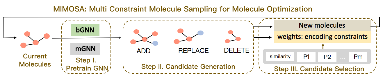
Figure 1: The Multi-constraint Molecule Sampling for Molecule Optimization(MIMOSA) framework illustrated using a single molecule. In Step I (Pretrain GNN), MIMOSA pretrains two property-agnostic GNNs for molecule topology and substructure-type prediction. Then, in Step II (Candidate Generation), MIMOSA uses the prediction and employs three basic substructure operations (ADD, REPLACE and DELETE) to generate new molecule candidates. In Step III (Candidate Selection), MIMOSA assigns weights for new molecule. The weights can encode multiple constraints including similarity and drug property constraints, upon which we accept promising molecules for next iteration. MIMOSA iteratively edits the molecule and can efficiently draw molecule samples.

Fig. 1 illustrates the overall procedure of MIMOSA, which can be decomposed into the following steps: (1) Pretrain GNN. MIMOSA pre-trains two graph neural networks (GNNs) using a large number of unlabeled molecules, which will be used in the sampling process. Then MIMOSA iterates over the following two steps. (2) Candidate Generation. We generate and score molecule candidates via modification operations (add, delete, replace) to the current molecule. (3) Candidate Selection. We perform MCMC sampling to select promising molecule candidates for the next sampling iteration by repeating Step 2 and 3. Note that all modification operations are on the substructure level, where a substructure can be either an atom or a single ring. The substructure set includes all 118 atoms and 31 single rings.

(I) Pretrain GNNs for Substructure-type and Molecule Topology Prediction

To provide accurate molecule representation, we propose to pretrain molecule embeddings on large molecule datasets. Since we consider molecules in graph representations where each substructure is a node, we develop two GNN based pretraining tasks to assist molecule modification. These two GNNs will assess the probability of each substructure conditioned on all the other substructures in the molecule graph.

Mathematically, in molecular graph $Y=(V,E)$, we have one-hot node feature $\mathbf{f}_{v}\in\{0,1\}^{C_{1}}$ for every node $v\in V$ and one-hot edge feature $\mathbf{g}_{e}\in\{0,1\}^{C_{2}}$ for every edge $e=(u,v)\in E$. $C_{1}$ and $C_{2}$ are the number of substructures and the number of bond types, respectively. In our experiment, $C_{1}=149$, including 118 atoms, 31 single rings, and $C_{2}=4$ correspond to the four bond types. We list the node and edge features in the appendix.

The two Graph Neural Networks (GNN)  [15] are learned with these node and edge features and the same molecule graph to learn an embedding vector $\mathbf{h}_{v}$ for every node $v\in V$.

$$\mathbf{h}_{v}^{(k)}= \mathrm{ReLU}\bigg{(}\mathrm{MLP}\Big{(}\mathrm{CONCAT}$$ (3)

$$\ \big{(}\sum_{u\in\mathcal{N}(v)\cup\{v\}}\mathbf{h}_{u}^{(k-1)},\sum_{e=(u,v):u\in\mathcal{N}(v)}\mathbf{g}_{e}^{(k-1)}\big{)}\Big{)}\bigg{)},\ \$$

where the layer $k=1,\cdots,K$; $\text{CONCAT}(\cdot,\cdot)$ is the concatenation of two vectors; $\mathcal{N}(v)$ is the set of all neighbors of $v$; $\mathbf{h}_{v}^{(0)}$ is the initial node embedding $\mathbf{f}_{v}$. After $K$ layers of GNN, we have the final node embedding $\mathbf{h}_{v}^{(K)}$ for node $v$. In our experiment, $K=5$.

Using the same GNN architecture, we trained two GNN models: one for substructure-type prediction called mGNN and one for molecule topology prediction called bGNN: We choose to train two separate GNNs instead of sharing a single GNN because sufficient unlabeled molecule samples exist and the two tasks are very different in nature.

The mGNN model aims at multi-class classification for predicting the substructure type of a masked node. The mGNN model outputs the type of an individual substructure conditioned on all other substructures and their connections. We mask the individual substructure, replace it with a special masked indicator following [15]. Suppose we only mask one substructure for each molecule during training and $v$ is the masked substructure (i.e., node), $y_{v}$ is the node label corresponding to masked substructure type, we add fully-connected (FC) layers with softmax activation (Eq. (4)) to predict the type of the node $v$.

$$\mathbf{\hat{y}}_{v}=\mathrm{Softmax}\big{(}\mathrm{FC}(\mathbf{h}_{v}^{(K)})\big{)}.$$ (4)

where $\mathbf{\hat{y}_{v}}$ is a $C_{1}$ dimension vector, indicating the predicted probability of all possible substructures. Multi-class cross entropy loss (Eq. (5)) is used to guide the training of GNN:

$$\mathcal{L}(\mathbf{y}_{v},\mathbf{\hat{y}}_{v})=-\sum_{i=1}^{C_{1}}\big{(}(\mathbf{y}_{v})_{i}\log(\mathbf{\hat{y}}_{v})_{i}\big{)},$$ (5)

where $\mathbf{y}_{v}$ is the groundtruth, one-hot vector. $C_{1}$ is number of all substructures (atoms and single rings), $(\mathbf{y}_{v})_{i}$ is i-th element of vector $\mathbf{y}_{v}$.

To summarize, the prediction of mGNN is defined as

$$\mathbf{\hat{y}}_{v}\triangleq\text{mGNN}(Y,\text{mask}=v)=\text{mGNN}(Y,v),$$ (6)

where in a given molecule $Y$ the node $v$ is masked, mGNN predicts the substructure distribution on masked node $v$, which is denoted $\mathbf{\hat{y}}_{v}$.

The bGNN model aims at binary classification for predicting the molecule topology. The goal of bGNN is to predict whether a node will expand. To provide training labels for bGNN, we set the leaf nodes (nodes with degree 1) with label $z_{v}=0$ as we assume they are no longer expanding. And we set label $z_{v}=1$ on the non-leaf nodes that are adjacent to leaf nodes as those nodes expanded (to the leaf nodes). The prediction is done via

$$\hat{z}_{v}=\mathrm{Sigmoid}\big{(}\mathrm{FC}(\mathbf{h}_{v}^{(K)})\big{)},$$ (7)

where FC is two-layer fully-connected layers (of 50 neurons followed by 1 neuron). $\mathbf{h}_{v}^{(K)}$ is defined in Eq. (3), the node embedding of $v$ produced by GNN. Binary cross-entropy loss is used to guide the training:

$$\mathcal{L}(z_{v},\hat{z}_{v})=-z_{v}\log(\hat{z}_{v})-(1-z_{v})\log(1-\hat{z}_{v}).$$ (8)

Since the total number of unlabeled molecules is large, when training bGNN we randomly select one substructure $v$ for each molecule to speed up the pretraining.

In sum, prediction of bGNN is defined as

$$\hat{z}_{v}\triangleq\text{bGNN}(Y,v),$$ (9)

where v is a node in molecule $Y$, $\hat{z}_{v}$ is the probability that $v$ will expand.

(II) Candidate Generation via Substructure Modification Operation

With the help of mGNN and bGNN, we define substructure modification operations namely replace, add or delete on input molecule $Y$:

• Replace a substructure. At node $v$, the original substructure category is $s_{v}$.

  1. We mask $v$ in $Y$, evaluate the substructure distribution in $v$ via mGNN, i.e., $\mathbf{\hat{y}}_{v}=\text{mGNN}(Y,v),$ as Eq. (6).

  2. Then we sample a new substructure $s^{\prime}_{v}$ from the multinomial distribution $\mathbf{\hat{y}}_{v}$, denoted by $s^{\prime}_{v}\sim\text{Multinomial}(\mathbf{\hat{y}}_{v})$.

  3. At node $v$, we replace the original substructure $s_{v}$ with new substructure $s^{\prime}_{v}$ to produce the new molecule $Y^{\prime}$.

  The whole operation is denoted as

  $$Y^{\prime}\sim S_{\mathrm{replace}}(Y^{\prime}|Y).$$ (10)

• Add a substructure. Suppose we want to add a substructure as leaf node (denoted as $v$) connecting to an existing node $u$ in current molecule $Y$. The substructure category of $v$ is denoted $s_{v}$, which we want to predict.

  1. We evaluate the probability that node $u$ has a leaf node $v$ with help of bGNN in Eq. (9), i.e.,

     $$\hat{z}_{u}=\mathrm{bGNN}(Y,u)\in[0,1].$$

  2. Suppose the above prediction is to add a leaf node $v$. We then generate a new molecule $Y^{\prime}$ via adding $v$ to $Y$ via a new edge $(u,v)$.

  3. In $Y^{\prime}$, $s_{v}$, the substructure of $v$ is unknown. We will predict its substructure using mGNN, i.e., $\mathbf{\hat{y}}_{v}=\text{mGNN}(Y^{\prime},v)$, following Eq. (6).

  4. We sample a new substructure $s^{\prime}_{v}$ from the multinomial distribution $\mathbf{\hat{y}}_{v}$ and complete the new molecule $Y^{\prime}$.

  The whole operation is denoted as

  $$Y^{\prime}\sim S_{\mathrm{add}}(Y^{\prime}|Y).$$ (11)

• Delete a substructure. We delete a leaf node $v$ in current molecule $Y$. It is denoted

  $$Y^{\prime}\sim S_{\mathrm{delete}}(Y^{\prime}|Y).$$ (12)

In the MCMC process, $S_{*}(Y^{\prime}|Y)$ indicates the sequential sampling process from previous sample $Y$ to next sample $Y^{\prime}$. And the very first sample is the input $X$.

Handling Bond Types and Rings. Since the number of possible bonds are small (single, double, triple, aromatic), we enumerate all and choose the one with largest $p_{X}(Y)$. In some case, basic operation would generate invalid molecules. Based on the indicator function in target distribution in Eq. (1), the density is equal to 0. Thus, we perform validity check using RDKit [23] to filter out the new molecule graphs that are not valid. When adding/replacing a ring, there might be multiple choices to connect to its neighbor. We enumerate all possible choices and retain all valid molecules.

(III) Candidate Selection via MCMC Sampling

The set of generated candidate molecules can be grouped as three sets based on the type of substructure modification they received, namely, replace set $S_{\mathrm{replace}}$, add set $S_{\mathrm{add}}$, and delete set $S_{\mathrm{delete}}$. MIMOSA uses the Gibbs sampling [12], a particular type of MCMC, for molecule candidate selection. Gibbs sampling algorithm generates an instance from the distribution of each variable in sequential or random order [24], conditional on the current values of the other variables. Here molecules from the three sets will be sampled with different sampling weights. Their weights are designed to satisfy the detailed balance condition [4].

Sampling $S_{\mathrm{replace}}$. For molecules produced by the “replace” operation, the weight in sampling $w_{r}$ is given by Eq. (13).

$$w_{r}=\frac{p_{X}(Y^{\prime})\cdot[\text{mGNN}(Y,v)]_{s^{\prime}_{v}}}{p_{X}(Y)\cdot[\text{mGNN}(Y,v)]_{s_{v}}},$$ (13)

where $P_{X}(\cdot)$ is the unnormalized target distribution for optimizing $X$, defined in Eq. (1), $[\text{mGNN}(Y,v)]_{s_{v}}$ is the predicted probability of the substructure $s_{v}$ in the prediction distribution $\text{mGNN}(Y,v)$. The acceptance rate in the proposal is $\min\{1,w_{r}\}$. If the proposal is accepted, we use the new prediction $s^{\prime}_{v}$ to replace origin substructure $s_{v}$ in current molecule $Y$ and produce the new molecule $Y^{\prime}$.

Sampling $S_{\mathrm{add}}$. For molecules produced by the “add” operation, the weight in sampling is given by Eq. (14).

$$w_{a}=\frac{p_{X}(Y^{\prime})\cdot\text{bGNN}(Y,u)\cdot[\text{mGNN}(Y^{\prime},v)]_{s_{v}}}{p_{X}(Y)\cdot(1-\text{bGNN}(Y,u))},$$ (14)

where The acceptance rate in the proposal is $\min\{1,w_{a}\}$.

Sampling $S_{\mathrm{delete}}$. For these molecules produced by “delete” operation, the weight in sampling is given by Eq. (15).

$$w_{d}=\frac{p_{X}(Y^{\prime})\cdot\big{(}1-\text{bGNN}(Y^{\prime},u)\big{)}}{p_{X}(Y)\cdot\text{bGNN}(Y^{\prime},u)\cdot[\text{mGNN}(Y,v)]_{s_{v}}},$$ (15)

where $v$ is the deleted node, leaf node (with degree 1) in molecular graph of $Y$. $u$ and $v$ are connected in $Y$. The acceptance rate in the proposal is $\min\{1,w_{d}\}$.

Soft-constraint Encoding. For these operations, any number or type of constraints (e.g., here the similarity and drug property constraints) can be encoded in $p_{X}(Y)$ and $p_{X}(Y^{\prime})$ and thus reflected in the weights $w_{r},w_{a},w_{d}$.

For a single-chain MCMC, we construct the transition kernel as given by Eq. (16).

$$Y^{\prime}\sim\left\{\begin{aligned} &S_{\mathrm{replace}}(Y^{\prime}|\ Y),&\text{prob}\ \gamma_{1},\text{accept w.}\ \min\{1,w_{r}\},\\ &S_{\mathrm{add}}(Y^{\prime}|\ Y),&\text{prob.}\ \gamma_{2},\text{accept w.}\ \min\{1,w_{a}\},\\ &S_{\mathrm{delete}}(Y^{\prime}|\ Y),&\text{prob.}\ \gamma_{3},\text{accept w.}\ \min\{1,w_{d}\},\\ \end{aligned}\right.$$ (16)

where $\gamma_{1},\gamma_{2},\gamma_{3}\in\mathbb{R}_{+}$ are hyperparameters that determine the sampling probabilities from the three molecule sets. In Section 3.3, we show the transition kernel will leave the target distribution $p_{X}(Y)$ invariant for arbitrary $\gamma_{1},\gamma_{2},\gamma_{3}$ satisfying $\gamma_{1}+\gamma_{2}+\gamma_{3}=1$ and $\gamma_{2}=\gamma_{3}$. After molecules are sampled, they will be accepted with their corresponding acceptance probabilities related to $w_{r},w_{a},w_{d}$.

Algorithm 1 MIMOSA for Molecule Optimization

1:  Input: molecule $X$, # of Particle $N$, max # of sampling iter. $T_{\mathrm{max}}$, # of burn-in iter. $T_{\mathrm{burnin}}$

2:  Output: Generated molecules $\Phi$.

3:  # Step (I) Pretrain GNN

4:  Train mGNN (Eq.6), bGNN (Eq.9).  

5:  Candidate set $\Theta=\{X\}$, Output set $\Phi=\{\}$.

6:  for $\mathrm{iter}=1,\cdots,T_{\text{max}}$ do

7:     # Step (II) Candidate Generation.

8:     Candidate Pool $\Psi=\{\}$.

9:     for molecule $Z$ in $\Theta$ do

10:        Generate candidates $Z^{\prime}$ via editing $Z$ using substructure operations; validity check; add $Z^{\prime}$ in $\Psi$.     

11:     end for

12:     $\Theta=\{\}$.

13:     # Step (III) Candidate Selection.

14:     if $\mathrm{iter}<T_{\mathrm{burnin}}$ then

15:        Select $N$ molecules with highest density value (Eq. 1) from $\Psi$ and add them into $\Theta$.

16:     else

17:        Draw $N$ molecules from $\Psi$ using importance sampling ($\propto$ weight $w_{r}$ in Eq. (13), $w_{a}$ in Eq. (14) or $w_{d}$ in Eq. (15)) and add to $\Theta$.

18:     end if

19:     $\Phi=\Phi\cup\Theta$.

20:  end for

The MIMOSA method is summarized in Algorithm 1. To accelerate the sampling procedure, we also deploy a multi-chain strategy [25]: during each step, we use $N$ samples for each state, with each sample generating multiple proposals. Also, during burn-in period (Step 12 in Algorithm 1), we pick the molecules with highest density for efficiency [4]. We retain N proposals in iterative sampling.

3.3 Analysis of the MCMC Algorithm

Our MCMC method draws unbiased samples from the target distribution, i.e., exhibiting ergodicity and convergence. We defer the proofs of Lemma 1 and  2 to the appendix.

Theorem 1.

Suppose $\{Y_{1},Y_{2},\cdots,Y_{n}\}$ is the chain of molecules sampled via MCMC based on transition kernel defined in Eq. (16), with initial state $X$, then the Markov chain is ergodic with stationary distribution $p_{X}(Y)$ in Eq. (1). That is, empirical estimate (time average over $Y_{1},Y_{2},\cdots,Y_{n}$) is equal to target value (space average over $p_{X}(Y)$), i.e., $\lim\limits_{n\xrightarrow{}+\infty}\frac{1}{n}\sum_{i=1}^{n}f(Y_{i})=\int f(Y)p_{X}(Y)dY$ holds for any integratable function $f$.

Proof Sketch. We split the proof into Lemma 1 and  2. First, regarding the ergodicity, it is sufficient to prove the irreducibility, aperiodicity of the Markov chain (Lemma 1). Then, to show that $p_{X}(Y)$ is maintained invariant for the whole chain, in Lemma 2, following [4], we show that detailed balance condition holds for any neighboring samples ($Y_{i}$ and $Y_{i+1}$). Then we strengthen this results on the whole chain.

Lemma 1.

The Markov chain of the sampled molecules ($\{Y_{1},\cdots,Y_{n}\}$, starting at $X$, based on transition kernel in Eq. (16)) is ergodic over the target distribution $p_{X}(Y)$.

Lemma 2.

$p_{X}(Y)$ is maintained as the invariant distribution for the whole Markov chain produced by MCMC transition kernel defined in Eq. (16).

4 Experiment

4.1 Experimental Setup

Dataset and Molecular Properties. We use 2 million molecules from ZINC database [33, 15] to train both mGNN and bGNN. Following [35, 21, 37, 19, 11, 10, 9], we focus on the molecular properties below. For all scores, the higher the better.

• QED (Quantitative Estimate of Drug likeness) is an indicator of drug-likeness [2].

• DRD (Dopamine Receptor) measures a molecule’s biological activity against a biological target dopamine type 2 receptor [6].

• PLogP (Penalized LogP) is the log of the partition ratio of the solute between octanol and water minus the synthetic accessibility score and number of long cycles [8].

Note that PLogP is more sensitive to the change of local molecule structures, while DRD and QED are related to both local and global molecule structures. For chemically valid molecules, their QED, DRD2 and LogP scores can be evaluated via Therapeutic Data Common (TDC) [16] (using two lines of code, a python library).

Baseline Methods. We compare MIMOSA with the following molecule optimization baselines. The parameter setting of these methods are provided in the appendix.

• JTVAE (Junction Tree Variational Auto-Encoder) [18] is a generative model that learns latent space to generate desired molecule. It also uses an encoder-decoder architecture and leverage a junction tree to simplify molecule generation procedure.

• VJTNN (Variational Junction Tree Encoder-Decoder) [21] improves over JTVAE by leveraging adversarial learning and attention.

• GCPN (Graph Convolutional Policy Network) [35]. GCPN is state-of-the-art reinforcement learning based approach on molecule optimization. It leverages graph convolutional policy networks to generate molecular structures with specific property, where molecular property is included in reward.

• GA (Genetic Algorithm) [27] is a genetic algorithm that explores chemical space efficiently.

Details on Implementation, Features, Dataset Construction, Evaluation Strategies are in Appendix.

The code repository (including readme file, data preprocessing and model construction, evaluation) is available at https://github.com/futianfan/MIMOSA.

Metrics We consider the following metrics for evaluation.

• Similarity between the input and generated molecule, measured by Tanimoto similarity over Morgan fingerprints [32], defined in Eq. (2).

• Property Improvement of generated molecule in QED, DRD, and PLogP. It is defined as the difference of the property score between generated molecules $Y$ and input molecule $X$, i.e., $\text{property}(Y)-\text{property}(X)$.

• Success Rate (SR) based on similarity and property improvement between input molecule $X$ and generated molecule $Y$. We follow the same definitions of SR as in [21] (See details in appendix).

4.2 Results

Exp 1. Optimize Multiple Properties

To evaluate model performance on optimizing multiple drug properties, we consider the following combinations of property constraints:

(1) optimize QED (drug likeness) and PLogP (solubility);

(2) optimize DRD (biological activity against dopamine type 2 receptor ) and PLogP (solubility).

Table 2: Exp 1. Optimizing Multiple Properties.

Optimizing PLogP and QED
Method	Similarity	PLogP-Imp.	QED-Imp.	Success
JTVAE	0.16$\pm$0.08	0.14$\pm$0.27	0.01$\pm$0.10	0.4%
VJTNN	0.17$\pm$0.06	0.46$\pm$0.35	0.02$\pm$0.09	1.0%
GCPN	0.25$\pm$0.15	0.56$\pm$0.25	0.06$\pm$0.08	11.3%
GA	0.35$\pm$0.16	0.93$\pm$0.67	0.09$\pm$0.07	24.9%
MIMOSA	0.42$\pm$0.17	0.93$\pm$0.48	0.10$\pm$0.09	32.0%
Optimizing PLogP and DRD
Method	Similarity	PLogP-Imp.	DRD-Imp.	Success
JTVAE	0.18$\pm$0.08	0.20$\pm$0.18	0.18$\pm$0.09	0.8%
VJTNN	0.18$\pm$0.08	0.55$\pm$0.16	0.27$\pm$0.05	3.4%
GCPN	0.23$\pm$0.12	0.38$\pm$0.25	0.25$\pm$0.11	20.4%
GA	0.38$\pm$0.16	0.68$\pm$0.49	0.20$\pm$0.16	29.3%
MIMOSA	0.54$\pm$0.16	0.75$\pm$0.48	0.35$\pm$0.20	43.7%

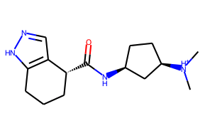
(a) Input Molecule $X$; QED:0.72; PLogP:-3.60

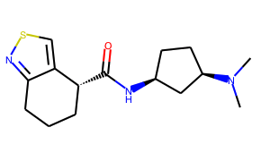
(b) sim: 0.66; QED: 0.93; PLogP: -1.2

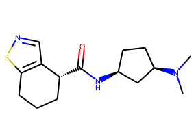
(c) sim: 0.59; QED: 0.93; PLogP: -1.1

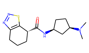
(d) sim: 0.57; QED: 0.92; PLogP:-1.6

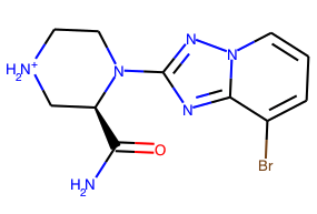
(e) Input Molecule $X$; QED: 0.71; PLogP: -3.9

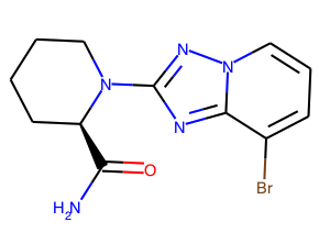
(f) sim: 0.837; QED: 0.90; PLogP: -0.6

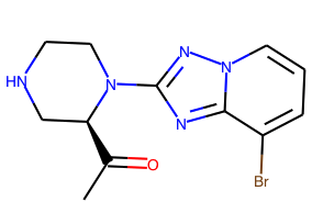
(g) sim: 0.872; QED: 0.89; PLogP: -1.2

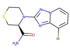
(h) sim: 0.812; QED: 0.88; PLogP: -1.4

Figure 2: Exp 3. Examples of “QED & PLogP” optimization. (Upper), the imidazole ring in the input molecule (a) is replaced by less polar rings thiazole (b and c) and thiadiazol (d). Since more polar indicates lower PLogP, the output molecules increase PLogP while maintaining the molecular scaffold. Lower), the PLogP of input molecule (e) is increased by neutralizing the ionized amine (g) or replacing with substructures with less electronegativity (f and h). These changes improve the QED.

From Table 2, MIMOSA has significantly better and stable performance on all metrics, with $28.5\%$ relative higher success rate in optimizing both QED and PLogP, and $49.1\%$ relative higher success rate in optimizing both DRD and PLogP compared with the second best algorithm GA. The GA algorithm uses genetic algorithm for local structure editing, hence is expected to work well on optimizing properties that are sensitive to local structural changes, such as joint optimizing both QED and PLogP where PLogP is related to the polarity of a molecule and is sensitive to the change of local structure. Because of the local editing of GA, GA does not perform well on optimizing both DRD and PLogP since DRD is less sensitive to the change of local structures. Among other baselines, GCPN has better performance. However, its performance is not stable when optimizing PLogP and QED simultaneously, since it can generate molecules with negative QED improvement.

Table 3: Exp 2. Optimizing Single Property.

Optimizing QED
Method	Similarity	QED-Improve	Success
JTVAE	0.30$\pm$0.09	0.17$\pm$0.12	17.4%
VJTNN	0.37$\pm$0.11	0.20$\pm$0.05	37.6%
GCPN	0.32$\pm$0.14	0.20$\pm$0.09	26.5%
GA	0.43$\pm$0.17	0.17$\pm$0.11	42.5%
MIMOSA	0.50$\pm$0.30	0.20$\pm$0.14	47.8%
Optimizing DRD
Method	Similarity	DRD-Improve	Success
JTVAE	0.31$\pm$0.07	0.34$\pm$0.17	25.6%
VJTNN	0.36$\pm$0.09	0.40$\pm$0.20	40.5%
GCPN	0.30$\pm$0.07	0.35$\pm$0.20	27.8%
GA	0.46$\pm$0.14	0.25$\pm$0.10	37.5%
MIMOSA	0.57$\pm$0.29	0.43$\pm$0.29	48.3%
Optimizing PLogP
Method	Similarity	PLogP-Improve	Success
JTVAE	0.30$\pm$0.09	0.28$\pm$0.17	2.9%
VJTNN	0.38$\pm$ 0.08	0.47$\pm$0.24	14.3%
GCPN	0.32$\pm$ 0.07	0.33$\pm$0.19	7.8%
GA	0.53$\pm$0.15	0.99$\pm$0.54	92.8%
MIMOSA	0.56$\pm$ 0.17	0.94$\pm$0.47	94.0%

Exp 2. Optimize Single Property

Since most baseline models were designed to optimize single drug properties, we also conduct experiments to compare MIMOSA with them on optimizing the following single properties: (1) DRD; (2) QED and (3) PLogP.

From the results shown in Table 3, we can see that when optimizing a single drug property, MIMOSA still achieved the best performance overall, with $12.5\%$ relative higher success rate in optimizing QED compared with the second best model GA, and $28.8\%$ relative higher success rate in optimizing both DRD compared with the second best algorithm VJTNN. Among the baseline models, algorithms such as JTVAE, VJTNN, and GCPN that were designed to optimize single property have good performance in property improvement as expected, however they generate molecules that have lower similarity hence the final success rates. Also, GA has the lowest QED and DRD improvement maybe due to its limitation in capturing global properties. High similarity between the output and input molecules is a unique requirement for the molecule optimization task, on which MIMOSA significantly outperformed the other baselines.

Exp 3. Case Study: Properties that are sensitive to local structural changes

To further examine how MIMOSA can also effectively improve properties that are sensitive to local structural change, e.g., PLogP, we show two examples in Fig. 2. For the first row, the imidazole ring in the input molecule (a) is replaced by less polar five-member rings thiazole (b and c) and thiadiazol (d). Since PLogP is related to the polarity of a molecule: more polar indicates lower PLogP. The generation results in the increase of PLogP while maintaining the molecular scaffold. For the second row, the PLogP of input molecule (e) is increased by neutralizing the ionized amine (g) or replacing with substructures with less electronegativity (f and h). These changes would also help improve the drug likeness, i.e., QED value.

Sampling Efficiency. The sampling complexity is $O(NN_{2})$ where $N$ the size of candidate set (e.g., 20) and $N_{2}$ is the size of the possible proposal set ($<$ 200). Empirically, this entire sampling process takes about 10-20 minutes for optimizing one source molecule, which is very acceptable for molecule optimization. And MCMC can directly operate with an unnormalized distribution which is more efficient. Note that all the existing methods for molecule optimization also utilize RDKit in their learning process, either in preprocessing steps for creating training data [18, 21], or inside their training procedure such as using RDKit to evaluate reward for reinforcement learning [35, 30, 37].

5 Conclusion

In this paper, we proposed MIMOSA, a new MCMC sampling based method for molecule optimization. MIMOSA pretrains GNNs and employs three basic substructure operations to generate new molecules and associated weights that can encode multiple drug property constraints, upon which we accept promising molecules for next iteration. MIMOSA iteratively produces new molecule candidates and can efficiently draw molecules that satisfy all constraints. MIMOSA significantly outperformed several state of the arts baselines for molecule optimization with 28.5% to 49.1% improvement when optimizing PLogP+QED, and PLogP+DRD, respectively.

Appendix

Proof of Lemma 1.

Proof.

For a Markov chain, to guarantee its ergodicity, it is sufficient to prove its irreducibility and aperiodicity [13].

Regarding irreducibility, without loss of generalization, we need to prove that any molecule pairs ($Y$, $Z$) can communicate with each other, i.e., $Y\leftrightarrow Z$. Both Y and Z are states of the Markov chain.

First, we want to show $Y\xrightarrow[]{}Z$, i.e., the state Y is accessible from state Z. This boils down to prove $\exists~{}n\in\mathbb{N}$ such that $P^{n}_{Y,Z}>0$. To show this, we construct such a Markov chain $\{Y_{0},Y_{1},\cdots,Y_{n}\}$, where $Y_{0}=Y$ and $Y_{n}=Z$.

First, we apply “delete” operation $n_{1}$ times to delete substructures of $Y$ until only one substructure is left, denoted C. That is, we have $Y_{i}\sim S_{\text{delete}}(Y_{i}|Y_{i-1})$ for $i=1,\cdots,n_{1}$. Based on acceptance rate defined in Eq. (15), we have $P^{1}_{Y_{i-1},Y_{i}}>0$ for $i=1,\cdots,n_{1}$. $Y_{0}=Y,Y_{n_{1}}=C$. We know $\exists~{}n_{1}\in\mathbb{N}$ such that

$$P^{n_{1}}_{Y,C}=P^{n_{1}}_{Y_{0},Y_{n_{1}}}=\prod_{i=1}^{n_{1}}P^{1}_{Y_{i-1},Y_{i}}>0.$$

Given this, we replace the substructure with a single substructure in $Z$, denoted as $C^{\prime}$, $Y_{n_{1}+1}\sim S_{\text{replace}}(Y_{n_{1}+1}|Y_{n_{1}}).$ Then starting with $C^{\prime}=Y_{n_{1}+1}$, we apply the “add” operation $n_{2}$ times until we have $Z$, then $Y_{i}\sim S_{\text{add}}(Y_{i}|Y_{i-1})$ for $i=n_{1}+2,\cdots,n_{1}+n_{2}+1.$ where $Y_{n_{1}+1}=C^{\prime},Y_{n_{1}+n_{2}+1}=Z$. Based on Eq. (14), we have $P^{1}_{Y_{i-1},Y_{i}}>0$ for $i=n_{1}+2,\cdots,n_{1}+n_{2}+1.$ $\exists~{}n_{2}\in\mathbb{N}$ such that

$$P^{n_{2}}_{C^{\prime},Z}=P^{n_{2}}_{Y_{n_{1}+1},Y_{n_{1}+n_{2}+1}}=\prod_{i=n_{1}+2}^{n_{1}+n_{2}+1}P^{1}_{Y_{i-1},Y_{i}}>0.$$

Thus, we have $n=(n_{1}+n_{2})\in\mathbb{N}$ s.t. $P^{n}_{Y,Z}=P^{n_{1}+n_{2}+1}_{Y,Z}\geq P^{n_{1}}_{Y,C}\cdot P^{1}_{C,C^{\prime}}\cdot P^{n_{2}}_{C,Z}>0.$

Similarly, we can show $Z\xrightarrow[]{}Y$, i.e., $\exists~{}n\in\mathbb{N}$ for $P^{n}_{Z,Y}>0$.

Now we have proved $Z\leftrightarrow Y$ hold for any molecule pairs $(Y,Z)$. Thus, we have proved irreducibility.

Next, for aperiodicity, there is a simple test: in Markov chain if there is a state $Y$ for which the 1-step transition probability $p(Y,Y)>0$, then the chain is aperiodic [13]. In MIMOSA scenario, the substructure type prediction is defined in Eq. (6), since it’s softmax output, so for each possible substructure the probability is bounded away from zero and one. The topology prediction is defined in Eq. (9), since it’s sigmoid output, the probability is also bounded away from zero and one. Thus, there exists such a molecule whose the acceptance probability is lower than 1, i.e., possible to reject the proposal, that is the 1-step transition probability is greater than 0, so aperiodicity satisfies.

∎

Proof of Lemma 2.

Proof.

In MCMC, the detailed balance condition guarantees that $p(x)\mathcal{T}(x\xrightarrow{}y)=p(y)\mathcal{T}(y\xrightarrow{}x),$ where $p(\cdot)$ is the target distribution for drawing samples, $\mathcal{T}(\cdot\xrightarrow{}\cdot)$ is the transition kernel from one state to another.

Below we first show for all three proposals detailed balance condition holds for any neighboring samples ($Y_{i-1}$ and $Y_{i}$), then we strengthen this conclusion on the whole Markov chain.

For “replace” proposal, we have

$$p_{X}(Y)\mathcal{T}(Y\xrightarrow{}Y^{\prime})$$ (17)

$$= p_{X}(Y)\cdot[\mathrm{mGNN}(Y,v)]_{s_{v}}\cdot\min\{1,w_{r}\}$$

$$= p_{X}(Y)\cdot[\mathrm{mGNN}(Y,v)]_{s_{v}}$$

$$\cdot\min\bigg{\{}1,\frac{p_{X}(Y^{\prime})\cdot[\mathrm{mGNN}(Y,v)]_{s^{\prime}_{v}}}{p_{X}(Y)\cdot[\mathrm{mGNN}(Y,v)]_{s_{v}}}\bigg{\}}$$

$$= \min\bigg{\{}p_{X}(Y)\cdot[\mathrm{mGNN}(Y,v)]_{s_{v}},$$

$$\ \ \ \ p_{X}(Y^{\prime})\cdot[\mathrm{mGNN}(Y,v)]_{s^{\prime}_{v}}\bigg{\}}.$$

where we focus on replace operation on node $v$. At node $v$, $s_{v}$ and $s^{\prime}_{v}$ are the actual and predicted substructure labels, respectively. $w_{r}$ is defined in Eq. (13).

$$w_{r}=\frac{p_{X}(Y^{\prime})\cdot[\text{mGNN}(Y,v)]_{s^{\prime}_{v}}}{p_{X}(Y)\cdot[\text{mGNN}(Y,v)]_{s_{v}}},$$ (18)

For the other direction, the following equation that shows detailed balance hold for “replace” proposal.

$$p_{X}(Y^{\prime})\mathcal{T}(Y^{\prime}\xrightarrow{}Y)$$ (19)

$$= p_{X}(Y^{\prime})\cdot[\mathrm{mGNN}(Y,v)]_{s^{\prime}_{v}}\cdot\min\{1,w^{\prime}_{r}\}$$

$$= p_{X}(Y^{\prime})\cdot[\mathrm{mGNN}(Y,v)]_{s^{\prime}_{v}}$$

$$\cdot\min\bigg{\{}1,\frac{p_{X}(Y)\cdot[\mathrm{mGNN}(Y,v)]_{s_{v}}}{p_{X}(Y^{\prime})\cdot[\mathrm{mGNN}(Y,v)]_{s^{\prime}_{v}}}\bigg{\}}$$

$$= \min\bigg{\{}p_{X}(Y^{\prime})\cdot[\mathrm{mGNN}(Y,v)]_{s^{\prime}_{v}},$$

$$\ \ \ \ p_{X}(Y)\cdot[\mathrm{mGNN}(Y^{\prime},v)]_{s_{v}}\bigg{\}}.$$

$$= p_{X}(Y)\mathcal{T}(Y\xrightarrow{}Y^{\prime})$$

Note that based on definition of mGNN in Eq. (6), during replace operation, we have

$$\mathrm{mGNN}(Y,v)=\mathrm{mGNN}(Y^{\prime},v)$$

We write $\mathrm{mGNN}(Y,v)$ instead of $\mathrm{mGNN}(Y^{\prime},v)$ for simplicity.

$w^{\prime}_{r}$ is the acceptance ratio from $Y^{\prime}$ to $Y$ and satisfy

$$w^{\prime}_{r}=\frac{p_{X}(Y)\cdot[\text{mGNN}(Y^{\prime},v)]_{s_{v}}}{p_{X}(Y^{\prime})\cdot[\text{mGNN}(Y^{\prime},v)]_{s^{\prime}_{v}}}=\frac{p_{X}(Y)\cdot[\text{mGNN}(Y,v)]_{s_{v}}}{p_{X}(Y^{\prime})\cdot[\text{mGNN}(Y,v)]_{s^{\prime}_{v}}},$$

For “add” proposal, we have

$$\ p_{X}(Y)\cdot\mathcal{T}(Y\xrightarrow{}Y^{\prime})$$ (20)

$$= \ p_{X}(Y)\cdot(1-\text{bGNN}(Y,u)))\min\{1,w_{a}\}$$

$$= \ p_{X}(Y)\cdot(1-\text{bGNN}(Y,u))$$

$$\ \ \cdot\min\bigg{\{}1,\frac{p_{X}(Y^{\prime})\cdot\text{bGNN}(Y,u)\cdot[\text{mGNN}(Y^{\prime},v)]_{s_{v}}}{p_{X}(Y)\cdot(1-\text{bGNN}(Y,u))}\bigg{\}}$$

$$= \ \min\bigg{\{}p_{X}(Y)\cdot(1-\text{bGNN}(Y,u)),$$

$$\ \ \ \ \ \ \ \ \ \ p_{X}(Y^{\prime})\cdot\text{bGNN}(Y,u)\cdot[\text{mGNN}(Y^{\prime},v)]_{s_{v}}\bigg{\}}$$

where $w_{a}$ is defined in Eq. (14).

$$w_{a}=\frac{p_{X}(Y^{\prime})\cdot\text{bGNN}(Y,u)\cdot[\text{mGNN}(Y^{\prime},v)]_{s_{v}}}{p_{X}(Y)\cdot(1-\text{bGNN}(Y,u))},$$ (21)

For the other direction, the equations below show detailed balance condition holds for “add” proposal.

$$\ p_{X}(Y^{\prime})\cdot\mathcal{T}(Y^{\prime}\xrightarrow{}Y)$$ (22)

$$= \ p_{X}(Y^{\prime})\cdot\text{bGNN}(Y,u)\cdot[\text{mGNN}(Y^{\prime},v)]_{s_{v}}\cdot\min\{1,w^{\prime}_{a}\}$$

$$= \ p_{X}(Y^{\prime})\cdot\text{bGNN}(Y,u)\cdot[\text{mGNN}(Y^{\prime},v)]_{s_{v}}$$

$$\cdot\min\bigg{\{}1,\frac{p_{X}(Y)\cdot(1-\text{bGNN}(Y,u))}{p_{X}(Y^{\prime})\cdot\text{bGNN}(Y,u)\cdot[\text{mGNN}(Y^{\prime},v)]_{s_{v}}}\bigg{\}}$$

$$= \ \min\bigg{\{}\ p_{X}(Y^{\prime})\cdot\text{bGNN}(Y,u)\cdot[\text{mGNN}(Y^{\prime},v)]_{s_{v}},$$

$$\ \ \ \ \ \ \ \ \ \ \ \ \ p_{X}(Y)\cdot(1-\text{bGNN}(Y,u))\bigg{\}}$$

where $w^{\prime}_{a}$ is the acceptance rate from $Y^{\prime}$ to $Y$ using delete operation, defined in Equation (15).

For the “delete” proposal, we can view it as the reverse procedure of the “add” proposal, which is easy to prove.

Since detailed balance holds for all proposals, i.e., $p_{X}(Y_{i})\mathcal{T}(Y_{i}\xrightarrow{}Y_{i-1})=p_{X}(Y_{i-1})\mathcal{T}(Y_{i-1}\xrightarrow{}Y_{i}),$ by integrating out $Y_{i-1}$ on both sides, we obtain

$$p_{X}(Y_{i})= \int p_{X}(Y_{i})\mathcal{T}(Y_{i}\xrightarrow{}Y_{i-1})dY_{i-1}$$ (23)

$$= \int p_{X}(Y_{i-1})\mathcal{T}(Y_{i-1}\xrightarrow{}Y_{i})dY_{i-1}$$

That is, distribution $p_{X}(\cdot)$ is stationary with a transition kernel $\mathcal{T}(\cdot\xrightarrow{}\cdot)$, i.e., $\mathcal{T}(p_{X})=p_{X}$ hold for transition kernel that contains “replace”, “add” or “delete” proposal.

∎

6 More Experimental Details

Implementation We implemented MIMOSA using Pytorch 1.0.1 and Python 3.7 on an Intel Xeon E5-2690 machine with 256G RAM and 8 NVIDIA Pascal Titan X GPUs. We use Adam optimizer with a learning rate of 0.001. For pretraining, we follow [15] to set GNNs with 5 layers and 300-d hidden units. For fully connected layer used in Equation (4) and  (7), we use two layer feedforward NN, the hidden size is 50. Tanimoto similarity, PLogP, and QED scores were computed using RDKit package [23]. The DRD2 activity prediction model is publicly available . For mGNN, we randomly mask a single node for each molecule, while for bGNN, we randomly select a leaf node for each molecule. When training them, we choose batch size 256, epochs number 10, and learning rate $1e^{-3}$, Then, during inference stage, we keep 20 molecules each iteration, i.e., in Algorithm 1, $N=20$. We set $T_{\text{max}}=10$ and $T_{\text{burnin}}=5$. When optimizing “QED+PLogP” and “DRD+PLogP” ($M=2$), for the target distribution $p_{X}(Y)$ (defined in Eq. (1)), we have $\eta_{0}=1.0$, $\eta_{1}=0.3$, and $\eta_{2}=0.3$.

Node and Edge Feature

In this paper, a substructure corresponds to a node, which contains 149 different types, including 118 atoms (e.g., Carbon, Nitrogen, Oxygen, Sulfur, etc) and 31 frequent single rings (e.g., Benzene, Cyclopropane). Each edge corresponds to a bond in molecular graph. There are totally 4 kinds of bonds, thus we have 4 edge type in total, including single, double, triple and aromatic.

Success Rate For LogP, we define a success as $\text{sim}(X,Y)\geq 0.4$ and $\text{PLogP}(Y)-\text{PLogP}(X)\geq 0.5$. For QED, we define a success as $\text{sim}(X,Y)\geq 0.4$ and $\text{QED}(Y)-\text{QED}(X)\geq 0.1$. For DRD, we define a success as $\text{sim}(X,Y)\geq 0.4$ and $\text{DRD}(Y)-\text{DRD}(X)\geq 0.2$. For optimizing both QED and PLogP , we define a success as (i) $\text{sim}(X,Y)\geq 0.3$, (ii) $\text{QED}(Y)-\text{QED}(X)\geq 0.1$, (iii) $\text{PLogP}(Y)-\text{PLogP}(X)\geq 0.3$. For optimizing both DRD and PLogP, we define a success as (i) $\text{sim}(X,Y)\geq 0.3$, (ii) $\text{DRD}(Y)-\text{DRD}(X)\geq 0.2$, (iii) $\text{PLogP}(Y)-\text{PLogP}(X)\geq 0.3$.

Baseline Setup Below are more detailed about baselines.

JTVAE. We follow [18] to use 780 substructures for junction tree, 5-layers message passing network as encoder. The hidden state dimension is set to 450. For the graph encoder, the initial atom features include its atom type, degree, its formal charge and its chiral configuration. Bond feature is a concatenation of its bond type, whether the bond is in a ring, and its cis-trans configuration. For the tree encoder, each cluster is represented with a neural embedding vector. The tree and graph decoder use the same feature setting as encoders. The graph encoder and decoder run three iterations of neural message passing. The code is publicly available from the author website . The paired molecules required in training JTVAE was obtained from from the author website .

VJTNN. We follow  [21] to set the hidden state dimension as 300 and latent code dimension as 8. The tree encoder runs message passing for 6 iterations, and graph encoder runs for 3 iterations. The hidden state dimension of the recurrent encoder and decoder is set to 600. We leverage the Adam optimizer for 20 epochs with learning rate 0.001. The learning rate is annealed by 0.9 for every epoch. For adversarial training, the discriminator has 3-layer and with hidden layer dimension 300 and LeakyReLU activation function. The code was obtained from the author website .

GCPN. We follow  [35] to set up an OpenAI Gym environment using RDKit package. The maximum atom number is 38. Since we represent molecules in kekulized form, there are 9 atom types and 3 edge types. We use a 3-layer GCPN as the policy network with 64 dimensional node embedding in all hidden layers. Batch normalization is applied after each layer. We use Adam optimizer with batch size 32. The learning rate is set as 0.001. The code was publicly available the author website .

GA. we follow [27] to run each experiment for 20 generations with a population size of 500. We compute the number of experiments that successfully proposed molecules with a squared difference less than 1.0. Each run is constrained to run for 100 generations with a maximum canonical SMILES length of 81 characters. The code was obtained from the author website.

References

- [1] Igor Baskin and Alexandre Varnek. Fragment descriptors in sar/qsar/qspr studies, molecular similarity analysis and in virtual screening. ChemInform, 40(20):i, 2009.
- [2] G Richard Bickerton, Gaia V Paolini, Jérémy Besnard, Sorel Muresan, and Andrew L Hopkins. Quantifying the chemical beauty of drugs. Nature chemistry, 4(2):90, 2012.
- [3] T. Blaschke, M. Olivecrona, O. Engkvist, J. Bajorath, and H. Chen. Application of generative autoencoder in de novo molecular design. Mol. Inform., 2018.
- [4] Steve Brooks, Andrew Gelman, Galin Jones, and Xiao-Li Meng. Handbook of markov chain monte carlo. CRC press, 2011.
- [5] Nicola De Cao and Thomas Kipf. Molgan: An implicit generative model for small molecular graphs, 2018.
- [6] DE Comings, D Muhleman, and R Gysin. Dopamine d2 receptor (drd2) gene and susceptibility to posttraumatic stress disorder: a study and replication. Biological psychiatry, 40(5):368–372, 1996.
- [7] Hanjun Dai, Yingtao Tian, Bo Dai, Steven Skiena, and Le Song. Syntax-directed variational autoencoder for structured data. arXiv preprint arXiv:1802.08786, 2018.
- [8] Peter Ertl and Ansgar Schuffenhauer. Estimation of synthetic accessibility score of drug-like molecules based on molecular complexity and fragment contributions. Journal of cheminformatics, 1(1):8, 2009.
- [9] Tianfan Fu, Wenhao Gao, Cao Xiao, Jacob Yasonik, Connor W Coley, and Jimeng Sun. Differentiable scaffolding tree for molecular optimization. International Conference on Learning Representations, 2022.
- [10] Tianfan Fu, Cao Xiao, Lucas Glass, and Jimeng Sun. -mop: Molecule optimization with -divergence. BIBM, 2020.
- [11] Tianfan Fu, Cao Xiao, Cheng Qian, Lucas M Glass, and Jimeng Sun. Probabilistic and dynamic molecule-disease interaction modeling for drug discovery. In Proceedings of the 27th ACM SIGKDD Conference on Knowledge Discovery & Data Mining, pages 404–414, 2021.
- [12] Stuart Geman and Donald Geman. Stochastic relaxation, gibbs distributions, and the bayesian restoration of images. IEEE Transactions on pattern analysis and machine intelligence, 6:721–741, 1984.
- [13] Walter R Gilks. Markov Chain Monte Carlo. Encyclopedia of biostatistics, 4, 2005.
- [14] Rafael Gómez-Bombarelli, Jennifer N Wei, David Duvenaud, José Miguel Hernández-Lobato, Benjamín Sánchez-Lengeling, Dennis Sheberla, Jorge Aguilera-Iparraguirre, Timothy D Hirzel, Ryan P Adams, and Alán Aspuru-Guzik. Automatic chemical design using a data-driven continuous representation of molecules. ACS central science, 4(2):268–276, 2018.
- [15] Weihua Hu, Bowen Liu, Joseph Gomes, Marinka Zitnik, Percy Liang, Vijay Pande, and Jure Leskovec. Strategies for pre-training graph neural networks. In ICLR, 2019.
- [16] Kexin Huang et al. Therapeutics data commons: machine learning datasets and tasks for therapeutics. NeurIPS Track Datasets and Benchmarks, 2021.
- [17] Kexin Huang, Tianfan Fu, Dawood Khan, Ali Abid, Ali Abdalla, Abubakar Abid, Lucas M Glass, Marinka Zitnik, Cao Xiao, and Jimeng Sun. Moldesigner: Interactive design of efficacious drugs with deep learning. NEURIPS Demo, 2020.
- [18] Wengong Jin, Regina Barzilay, and Tommi Jaakkola. Junction tree variational autoencoder for molecular graph generation. ICML, 2018.
- [19] Wengong Jin, Regina Barzilay, and Tommi Jaakkola. Multi-resolution autoregressive graph-to-graph translation for molecules. arXiv preprint arXiv:1907.11223, 2019.
- [20] Wengong Jin, Regina Barzilay, and Tommi Jaakkola. Composing molecules with multiple property constraints. arXiv preprint arXiv:2002.03244, 2020.
- [21] Wengong Jin, Kevin Yang, Regina Barzilay, and Tommi Jaakkola. Learning multimodal graph-to-graph translation for molecular optimization. ICLR, 2019.
- [22] Matt J Kusner, Brooks Paige, and José Miguel Hernández-Lobato. Grammar variational autoencoder. In ICML, pages 1945–1954. JMLR. org, 2017.
- [23] Greg Landrum et al. Rdkit: Open-source cheminformatics, 2006.
- [24] Richard A Levine and George Casella. Optimizing random scan gibbs samplers. Journal of Multivariate Analysis, 97(10):2071–2100, 2006.
- [25] Jun S Liu, Faming Liang, and Wing Hung Wong. The multiple-try method and local optimization in metropolis sampling. Journal of the American Statistical Association, 95(449):121–134, 2000.
- [26] Qi Liu, Miltiadis Allamanis, Marc Brockschmidt, and Alexander Gaunt. Constrained graph variational autoencoders for molecule design. In Advances in Neural Information Processing Systems, pages 7795–7804, 2018.
- [27] AkshatKumar Nigam, Pascal Friederich, Mario Krenn, and Alan Aspuru-Guzik. Augmenting genetic algorithms with deep neural networks for exploring the chemical space. In ICLR, 2020.
- [28] Marcus Olivecrona, Thomas Blaschke, Ola Engkvist, and Hongming Chen. Molecular de-novo design through deep reinforcement learning. J. Cheminform., 9(1):48, September 2017.
- [29] Pavel G Polishchuk, Timur I Madzhidov, and Alexandre Varnek. Estimation of the size of drug-like chemical space based on gdb-17 data. Journal of computer-aided molecular design, 27(8):675–679, 2013.
- [30] Mariya Popova, Olexandr Isayev, and Alexander Tropsha. Deep reinforcement learning for de novo drug design. Science advances, 4(7):eaap7885, 2018.
- [31] E. Putin. Reinforced adversarial neural computer for de novo molecular design. J. Chem. Inf. Model., 2018.
- [32] David Rogers and Mathew Hahn. Extended-connectivity fingerprints. Journal of Chemical Information and Modeling, 50(5):742–754, 2010.
- [33] Teague Sterling and John J Irwin. Zinc 15–ligand discovery for everyone. Journal of chemical information and modeling, 55(11):2324–2337, 2015.
- [34] Max Welling and Yee W Teh. Bayesian learning via stochastic gradient langevin dynamics. In ICML, pages 681–688, 2011.
- [35] Jiaxuan You, Bowen Liu, Rex Ying, Vijay Pande, and Jure Leskovec. Graph convolutional policy network for goal-directed molecular graph generation. In NIPS, 2018.
- [36] Alex Zhavoronkov. Artificial intelligence for drug discovery, biomarker development, and generation of novel chemistry, 2018.
- [37] Zhenpeng Zhou, Steven Kearnes, Li Li, Richard N Zare, and Patrick Riley. Optimization of molecules via deep reinforcement learning. Scientific reports, 9(1):10752, 2019.