Testing homogeneity in dynamic discrete games in finite samples

Abstract

The literature on dynamic discrete games often assumes that the conditional choice probabilities and the state transition probabilities are homogeneous across markets and over time. We refer to this as the “homogeneity assumption” in dynamic discrete games. This assumption enables empirical studies to estimate the game’s structural parameters by pooling data from multiple markets and from many time periods. In this paper, we propose a hypothesis test to evaluate whether the homogeneity assumption holds in the data. Our hypothesis test is the result of an approximate randomization test, implemented via a Markov chain Monte Carlo (MCMC) algorithm. We show that our hypothesis test becomes valid as the (user-defined) number of MCMC draws diverges, for any fixed number of markets, time periods, and players. We apply our test to the empirical study of the U.S. Portland cement industry in Ryan (2012).

Keywords and phrases: Dynamic discrete choice problems, dynamic games, Markov decision problems, randomization tests, Markov chain Monte Carlo (MCMC).

JEL classification: C12, C57, C63

1 Introduction

In applications of dynamic discrete games, practitioners often assume that the conditional choice probabilities and the state transition probabilities are invariant across time and markets. We refer to this as the “homogeneity assumption” in dynamic discrete games. This is a convenient assumption, as it allows the estimation of the model’s structural parameters by pooling data from multiple markets and from many time periods.

Despite the widespread use of the homogeneity assumption in dynamic discrete games, it is plausible for this condition to fail in applications. We now provide a few examples. First, a game could suffer from a structural break in the model, which would invalidate the homogeneity assumption across time. Second, markets could be affected by persistent heterogeneity that is observed by the players but not by the researcher (e.g., Arcidiacono and Miller (2011)). This would invalidate the homogeneity assumption across markets. Third and relatedly, there may be multiplicity of equilibria, and different markets could be playing different equilibria. The literature has considered hypothesis testing for the multiplicity of equilibria in games. In particular, De Paula and Tang (2012) propose a test for the multiplicity of equilibria across markets in static games, while Otsu et al. (2016) do this in the context of dynamic games.

In this paper, we propose a hypothesis test for the homogeneity assumption. That is, our test is designed to capture the various possible violations to the homogeneity assumption described in the previous paragraph (both across markets and over time). Our test is implemented via Markov chain Monte Carlo (MCMC) methods, and it is justified by the theory of randomization tests (cf. Lehmann and Romano, 2005, Section 15.2). While our MCMC test is not a standard randomization test, we establish its validity by coupling it with an underlying randomization test that is valid in finite samples yet computationally infeasible in practically relevant applications. Our contribution is to show that the distribution generated by our MCMC algorithm approximates the underlying randomization test as the number of (user-defined) MCMC draws diverges. In this sense, we interpret our proposed MCMC algorithm as a computationally feasible way to implement a computationally infeasible underlying randomization test. It is worth mentioning that our results hold for any fixed and finite number of players, markets, and time periods, i.e., valid in finite samples. This is an important aspect of our contribution, as the datasets used in empirical applications often have a small number of time periods and markets. For example, our empirical application is based on Ryan (2012), and has only $n=23$ markets and either $T=9$ or $T=10$ time periods.

Our methodology is especially well suited for our testing problem in dynamic discrete games. As with standard randomization tests, the quality of our test depends on the richness of possible transformations exploited by our MCMC algorithm. There are three aspects of the typical framework in dynamic discrete games that allow us to generate a rich set of such transformations. First, dynamic discrete game models often impose independence across markets and have a Markovian structure. This provides the basis for our randomization-based methodology. Second, the data used in dynamic discrete games are usually either naturally discrete or discretized by the researcher. This is important for our test, as it relies on transformations defined by “conditional” permutations of data, i.e., permutations of the value of the state and the action across markets or time periods for which other related states coincide. Third, dynamic discrete game models often assume that actions are independent conditional on the state. This allows us to simplify the implementation of the transformations that generate our randomization-based methodology. It is worth pointing out that our inference methodology should apply to economic problems beyond the dynamic discrete game setup provided that these three aspects hold.

The econometric framework considered in this paper is arguably very general. It includes the single-agent dynamic discrete choice model (e.g., Rust (1987); Hotz and Miller (1993); Hotz et al. (1994); Aguirregabiria and Mira (2002)) and the Markov equilibrium dynamic game model (e.g., Pakes et al. (2007); Aguirregabiria and Mira (2007); Bajari et al. (2007); Pesendorfer and Schmidt-Dengler (2008, 2010)). Furthermore, it includes the Markov dynamic game model of Aguirregabiria and Magesan (2020), which allows some players to have biased beliefs. Importantly, our methodology does not impose functional forms on the primitive structure of the dynamic game (e.g., utility functions, state transition functions, etc.). We consider this advantageous, as functional form assumptions are hard to justify solely based on economic arguments, and are thus prone to misspecification.

In a recent paper, Otsu et al. (2016) propose several hypothesis tests for dynamic discrete games. Two of their proposals are directly related to the problem considered in our paper. Specifically, they consider a method to test the homogeneity across markets of the conditional choice probabilities and the state transition probabilities, under the maintained assumption that these functions are time-homogeneous. Their inference method is based on the bootstrap, and its validity is shown in an asymptotic framework in which the number of time periods $T$ diverges to infinity. However, the number of time periods in applications is often small. Besides the aforementioned application of Ryan (2012) with $T=9$ or $T=10$, we can mention Sweeting (2011) with $T=4$, Collard-Wexler (2013) with $T=24$, and Dunne et al. (2013) with $T=5$.

The most critical step of our MCMC algorithm is based on the so-called Euler Algorithm, described in Kandel et al. (1996). In related work, Besag and Mondal (2013) use the Euler Algorithm to test whether a time series of data has a time-homogeneous Markov structure. In terms of our setup, Besag and Mondal (2013)’s paper corresponds to testing whether the data from a single market has a time-homogeneous state transition probability. Relative to this work, our paper incorporates several essential features of dynamic Markov discrete games. First, we recognize that the dataset in a typical dynamic game has information about actions and states. Second, our construction exploits the typical economic structure imposed in dynamic games, such as the conditional independence assumption (i.e., conditional on the current state variable, the current action variable is independent from the past information). Finally, while Besag and Mondal (2013) focus on data from a single market, our MCMC algorithm exploits the possibility that the data includes observations from multiple markets. This is an important aspect of our contribution, as the datasets used in empirical applications usually include from data multiple markets, e.g., Ryan (2012) with $n=23$, Sweeting (2011) with $n=102$, Collard-Wexler (2013) with $n=1,600$, and Dunne et al. (2013) with $n=639$.

We explore the performance of our hypothesis test in Monte Carlo simulations. Our results show that our method provides excellent size control even in small samples, and can successfully detect relatively small deviations from the homogeneity hypothesis. In these two accounts, our test appears to work favorably in comparison with the bootstrap-based test in Otsu et al. (2016). These favorable results appear to extend even when the discrete data have many support points, which is common in applications. In our empirical application, we investigate the homogeneity of the decisions in the U.S. Portland cement industry data used in Ryan (2012). This is a key assumption in Ryan (2012), as it allows him to pool data from multiple markets to estimate the model’s parameters. Unlike Otsu et al. (2016)’s test, our test finds no evidence against the homogeneity hypothesis in the data. We implement our test using the Julia package HomogeneityTestBBU, which is publicly available at the GitHub repository.

The rest of the paper is organized as follows. Section 2 describes the dynamic discrete choice model and the hypothesis test. Section 3 specifies our hypothesis test and its implementation via our MCMC algorithm. Section 4 establishes the main theoretical results of the paper. The main technical insight is that our hypothesis test is an approximate way of implementing an underlying randomization test that is finite-sample valid yet computationally infeasible. Section 5 provides the empirical application. In Section 6, we evaluate the performance of our test in finite samples via Monte Carlo simulations. Section 7 concludes. The paper’s appendix collects all of the proofs, auxiliary results, and computational details related to our proposed MCMC algorithm.

2 Setup

2.1 The econometric model

We begin by describing the dynamic discrete game under consideration. We observe the outcome of $n$ markets in which $J$ players choose actions over $T$ time periods. Our setup allows for $J=1$, i.e., single-agent problems, or $J>1$, i.e., multiple-agent games. This paper’s inference results are valid for all finite $n$, $T$, and $J$.

We consider a setup in which the observed actions and state variables are discretely distributed. For every market $i=1,\ldots,n$ and period $t=1,\ldots,T$, let $A_{i,t}$ be the random variable that specifies the actions chosen by the players in market $i$ and period $t$, and let $S_{i,t}$ be the random variable that specifies the state variable of market $i$ and period $t$. We use $\mathcal{S}$ to denote the common support of $S_{i,t}$ and $\mathcal{A}$ to denote the common support of $A_{i,t}$. We define the following $n\times T$ matrices:

$$S ~{}\equiv~{}(S_{i,t}:i=1,\ldots,n,t=1,\ldots,T),$$

$$A ~{}\equiv~{}(A_{i,t}:i=1,\ldots,n,t=1,\ldots,T).$$

In this notation, the data are then given by

$$X~{}\equiv~{}(S,A).$$

By definition, the support of $X$ is given by $\mathcal{X}\equiv\mathcal{S}^{nT}\times\mathcal{A}^{nT}$.

Remark 2.1.

We assume a balanced panel (i.e., all $n$ markets are fully observed over $T$ time periods) only for the simplicity of notation and exposition. Our arguments extend immediately to the case in which each market $i=1,\dots,n$ is observed over a market-specific time period $T_{i}$.

The following assumption is standard in much of the literature on dynamic discrete games.

Assumption 2.1.

The following conditions hold:

1. $((S_{i,t},A_{i,t}):t=1,\ldots,T)$ are independent across $i=1,\ldots n$.

2. $(S_{i,t},A_{i,t})$ and $(S_{i,1},A_{i,1},\ldots,S_{i,t-2},A_{i,t-2})$ are conditionally independent given $(S_{i,t-1},A_{i,t-1})$ for every $i=1,\ldots,n$ and $t=3,\ldots,T$.

3. $A_{i,t}$ and $(S_{i,t-1},A_{i,t-1})$ are conditionally independent given $S_{i,t}$ for every $i=1,\ldots,n$ and $t=2,\ldots,T$.

Assumption 2.1 has three parts. Assumption 2.1(a) imposes that markets are independently distributed. Assumption 2.1(b) indicates that the observations of state and actions are a Markov process. Assumption 2.1(c) imposes that the current actions are independent of past information once we condition on the current state. Assumptions 2.1(b)-(c) are high-level restrictions that are typically imposed on the equilibrium strategies used by the players. In particular, they follow from the assumption that players use Markov strategies (e.g., see Maskin and Tirole (2001)), as assumed in Pakes et al. (2007); Aguirregabiria and Mira (2007); Bajari et al. (2007); Pesendorfer and Schmidt-Dengler (2008). These conditions are implied even in models in which the players’ beliefs are allowed to be out of equilibrium, i.e., do not coincide with the true equilibrium probabilities (e.g., Aguirregabiria and Magesan (2020)). Finally, we clarify that Assumption 2.1 refers to observed states and actions. As such, it may fail if there are state or action variables that are unobserved to the researcher and influence the distribution of their observed counterparts.

Assumption 2.1 is the only maintained assumption to study the validity of our hypothesis test. Notably, we do not impose functional forms on the primitive structure of the dynamic game, such as the utility functions, the state transition functions, or the discount factors. We view this as a virtue of our methodology, as these restrictions can be hard to justify based purely on economic arguments. Relatedly, while one could improve the statistical power of our test by exploiting functional form restrictions on the primitives of the dynamic game, they inevitably carry the risk of producing invalid inference when these are misspecified.

We now introduce necessary notation to express our hypothesis of interest. We use $\sigma_{i,t}$ to denote the conditional choice probability for market $i$ and period $t$, i.e., for every $(s,a)\in\mathcal{S\times A}$,

$$\sigma_{i,t}(a|s)~{}\equiv~{}P(A_{i,t}=a|S_{i,t}=s).$$

We use $f_{i,t+1}$ to denote the state transition probability from period $t$ to $t+1$ for market $i$, i.e., for every $(s,a,s^{\prime})\in\mathcal{S}\times\mathcal{A}\times\mathcal{S}$ ,

$$f_{i,t+1}(s^{\prime}|a,s)~{}\equiv~{}P(S_{i,t+1}=s^{\prime}|(S_{i,t},A_{i,t})=(s,a)).$$

Finally, we use $m_{i}(s)$ to denote the marginal state distribution for market $i$ in period 1, i.e., for every $s\in\mathcal{S}$,

$$m_{i}(s)~{}\equiv~{}P(S_{i,1}=s).$$

With this notation in place, we specify our hypothesis testing problem in the next section.

2.2 The hypothesis testing problem

Our goal is to test whether the “homogeneity assumption” holds in the data, i.e., whether the conditional choice probabilities and state transition probabilities are homogeneous across time and markets. That is,

$$H_{0}:\sigma_{i,t}(a|s)=\sigma(a|s)~{}~{}\text{and}~{}~{}f_{i,t+1}(s^{\prime}|a,s)=f(s^{\prime}|a,s).$$ (1)

Note that $H_{0}$ in (1) represents two types of homogeneity: time and market homogeneity, and involves two functions: conditional choice probabilities and state transition probabilities. In this sense, our hypothesis test evaluates four homogeneity conditions: time homogeneity of the conditional choice probabilities, market homogeneity of the conditional choice probabilities, time homogeneity of the state transition probabilities, and market homogeneity of the state transition probabilities. Under Assumption 2.1, a rejection of $H_{0}$ would be indicative that one or more of these homogeneity conditions is violated, suggesting it is not appropriate to pool data across markets and time periods.

As discussed in the introduction, there may be many possible reasons for the homogeneity assumption to fail. However, in general, it may be difficult to distinguish among the possible reasons. For example, given the recent literature on separately identifying equilibrium selection and market-specific permanent unobserved heterogeneity (Aguirregabiria and Mira, 2019; Luo et al., 2022), it may be difficult to distinguish between these two possible causes for failure of the homogeneity assumption. Nevertheless, in certain applications, one may feel comfortable that some of the conditions are satisfied and should be part of our maintained assumptions. For example, in a given application, one may be confident that the conditional choice probability and state transition probability are time homogeneous. Then, one could reinterpret $H_{0}$ as testing the market homogeneity of the conditional choice probabilities and state transition probabilities. To provide an additional example, if one is confident that market and time homogeneity holds for some subsets of the time periods (e.g., before and after a policy change), then $H_{0}$ may be reinterpreted as testing homogeneity of the conditional choice probabilities and state transition probabilities across the subsets of periods.

Under Assumption 2.1 and $H_{0}$, Lemma B.1 in the appendix shows that the likelihood of the data ${X}=({S},{A})$ evaluated at any realization $\tilde{X}=(\tilde{S},\tilde{A})\in\mathcal{X}$ is as follows:

$$P(X=\tilde{X})~{}=~{}\prod_{i=1}^{n}\left(m_{i}(\tilde{S}_{i,1})~{}\left(\prod_{t=1}^{T}\sigma(\tilde{A}_{i,t}|\tilde{S}_{i,t})\right)~{}\left(\prod_{{t}=1}^{T-1}f(\tilde{S}_{i,{t}+1}|\tilde{S}_{i,{t}},\tilde{A}_{i,{t}})\right)\right).$$ (2)

This expression reveals that the markets are independently distributed (Assumption 2.1(a)), but they are not necessarily identically distributed because $m_{i}(\cdot)$ depends on $i$. Even though the conditional choice probabilities and state transition probabilities are homogeneous under $H_{0}$, markets can still be heterogeneous due to differences in their initial state values. This is a desired feature in our testing problem, as the dynamic discrete choice literature usually allows the initial state distribution to be market-specific.

We conclude the section with an observation about the type of economic models considered in this paper. From an econometric viewpoint, our goal is to evaluate the homogeneity assumption (i.e., $H_{0}$ in (1)) using discrete data that satisfies Assumption 2.1. We motivated this problem using dynamic discrete choice games because they are an important class of models ideally suited to this econometric framework. However, it is worth highlighting that our methodology applies to any other discrete panel-data model that satisfies Assumption 2.1. We plan to consider alternative applications of our methodology in future research.

3 Our hypothesis test

In this paper, we propose to reject $H_{0}$ in (1) whenever the significance level $\alpha$ is larger than or equal to our $p$-value, which we denote by $\hat{p}_{K}$. That is,

$$\phi_{K}(X)~{}\equiv~{}1\{\hat{p}_{K}\leq\alpha\}.$$ (3)

In turn, our $p$-value $\hat{p}_{K}$ is the result of constructing $K$ transformations of the data via our MCMC algorithm, which is specified in Section 3.1. This MCMC algorithm produces $K$ sequential transformations of the data $X$, denoted by $(X^{(1)},\ldots,X^{(K)})$. Our $p$-value is then computed as follows

$$\hat{p}_{K}~{}\equiv~{}\frac{1}{K}\sum_{k=1}^{K}1\{\tau(X^{(k)})\geq\tau(X)\},$$ (4)

where $\tau:\mathcal{X}\to\mathbb{R}$ denotes the test statistic designed to detect departures from $H_{0}$ in the data.

One notable feature of our hypothesis test is that its validity does not depend on the choice of the test statistic (see Theorem 4.1). However, the power of our test depends critically on this choice. For reference, Example 3.1 specifies two test statistics considered in the related literature.

Example 3.1 (Test statistics $\tau(X)$).

Otsu et al. (2016, Eq. (4), (7)) propose the following statistics:

$$\tau_{1}(X) ~{}\equiv~{}\sum_{i=1}^{n}\sum_{(a,s)\in\mathcal{A}\times\mathcal{S}}(\hat{\sigma}_{i}(a|s)-\hat{\sigma}(a|s))^{2}\left(\frac{\sum_{t=1}^{T}1\{S_{i,t}=s\}}{\hat{\sigma}(a|s)}\right)$$

$$\tau_{2}(X) ~{}\equiv~{}2\sum_{i=1}^{n}\sum_{(a,s)\in\mathcal{A}\times\mathcal{S}}\hat{\sigma}_{i}(a|s)\ln\left(\frac{\hat{\sigma}_{i}(a|s)}{\hat{\sigma}(a|s)}\right)\sum_{t=1}^{T}1\{S_{i,t}=s\},$$ (5)

where we interpret $0/0=0$ and $0\times\ln(0)=0$, and we define

$$\hat{\sigma}_{i}(a|s) ~{}\equiv~{}\frac{\sum_{t=1}^{T}1\{A_{i,t}=a,S_{i,t}=s\}}{\sum_{t=1}^{T}1\{S_{i,t}=s\}}$$

$$\hat{\sigma}(a|s) ~{}\equiv~{}\frac{\sum_{i=1}^{n}\sum_{t=1}^{T}1\{A_{i,t}=a,S_{i,t}=s\}}{\sum_{i=1}^{n}\sum_{t=1}^{T}1\{S_{i,t}=s\}}.$$

These test statistics compare market-specific conditional choice probabilities with their pooled counterpart, so they are specifically designed to detect heterogeneity across markets.   

3.1 The MCMC algorithm

Our MCMC algorithm requires some notation. Let $I=(I_{1},I_{2})$ denote an arbitrary pair of markets $I_{1}$ and $I_{2}$ in the data, i.e., $I_{1},I_{2}\in\{1,2,\dots,n\}$. We allow for $I_{1}=I_{2}$. We use $\mathcal{I}$ to denote the collection of all such pairs of markets, i.e., $|\mathcal{I}|=n^{2}$. We also define several sets.

Definition 3.1 ($R_{S}(I,\breve{S})$).

For any $I=(I_{1},I_{2})\in\mathcal{I}$ and $\breve{S}\in\mathcal{S}^{nT}$, $R_{S}(I,\breve{S})$ is the set of all $\tilde{S}\in\mathcal{S}^{nT}$ satisfying the following conditions for all $s,s^{\prime}\in\mathcal{S}$:

1. $\tilde{S}_{i,1}=\breve{S}_{i,1}$ for all $i=1,\ldots,n$,

2. $\sum_{t=1}^{T-1}1\{\tilde{S}_{i,t}=s,\tilde{S}_{i,t+1}=s^{\prime}\}=\sum_{t=1}^{T-1}1\{\breve{S}_{i,t}=s,\breve{S}_{i,t+1}=s^{\prime}\}$ for all $i\not\in\{I_{1},I_{2}\}$,

3. $\sum_{i=I_{1},I_{2}}\sum_{t=1}^{T-1}1\{\tilde{S}_{i,t}=s,\tilde{S}_{i,t+1}=s^{\prime}\}=\sum_{i=I_{1},I_{2}}\sum_{t=1}^{T-1}1\{\breve{S}_{i,t}=s,\breve{S}_{i,t+1}=s^{\prime}\}$.

In words, $R_{S}(I,\breve{S})$ is the set of all state configurations that result from permuting the state data $\breve{S}$ subject to the restrictions in conditions (a)-(c), which we now interpret. First, condition (a) indicates that the initial value of the state variable must remain unchanged across markets. The reason behind this restriction is that our framework does not restrict the initial state distribution (i.e., $\{m_{i}(\tilde{S}_{i,1})\}_{i=1}^{n}$ in (2)). In turn, conditions (b)-(c) imply that the aggregate state transition frequencies across all markets $i=1,\dots,n$ must remain constant. This restriction is achieved by requiring the state transition frequencies to remain invariant for each market $i\not\in\{I_{1},I_{2}\}$ (by condition (b)) and on aggregate for markets $i\in\{I_{1},I_{2}\}$ (by condition (c)). The main reason behind breaking an aggregate restriction into conditions (b) and (c) is to keep $R_{S}(I,\breve{S})$ computationally tractable. Under Assumption 2.1 and $H_{0}$, the restrictions in conditions (a)-(c) imply that each state configuration in $R_{S}(I,\breve{S})$ has the same value of the likelihood function, provided that it is paired with a suitable action configuration. These suitable action configurations are precisely those in next definition.

Definition 3.2 ($R_{A}(\tilde{S},(\breve{S},\breve{A}))$).

For any $\tilde{S},\breve{S}\in\mathcal{S}^{nT}$ and $\breve{A}\in\mathcal{A}^{nT}$, $R_{A}(\tilde{S},(\breve{S},\breve{A}))$ is the set of all $\tilde{A}\in\mathcal{A}^{nT}$ satisfying the following conditions for all $s,s^{\prime}\in\mathcal{S}$ and $a\in\mathcal{A}$:

1. $\sum_{i=1}^{n}\sum_{t=1}^{T-1}1\{\tilde{S}_{i,t}=s,\tilde{A}_{i,t}=a,\tilde{S}_{i,t+1}=s^{\prime}\}=\sum_{i=1}^{n}\sum_{t=1}^{T-1}1\{\breve{S}_{i,t}=s,\breve{A}_{i,t}=a,\breve{S}_{i,t+1}=s^{\prime}\}$,

2. $\sum_{i=1}^{n}1\{\tilde{S}_{i,T}=s,\tilde{A}_{i,T}=a\}=\sum_{i=1}^{n}1\{\breve{S}_{i,T}=s,\breve{A}_{i,T}=a\}$.

By definition, $R_{A}(\tilde{S},(\breve{S},\breve{A}))$ is the set of action configurations that result from permuting the action data $\breve{A}$ subject to conditions (a)-(b), which we now explain. Condition (a) implies that the aggregate state and action transition frequencies across all markets $i=1,\dots,n$ remain constant. Condition (b) imposes an analogous requirement for the terminal period. Under Assumption 2.1 and $H_{0}$, these restrictions imply that the hypothetical data $(\breve{S},\breve{A})$ has the same likelihood as the state configuration $\tilde{S}$ paired with any action configuration in $R_{A}(\tilde{S},(\breve{S},\breve{A}))$.

Before explaining how $R_{S}(I,\breve{S})$ and $R_{A}(\tilde{S},(\breve{S},\breve{A}))$ are used in our MCMC algorithm, we illustrate their computation in a relatively simple example. While the conditions in Definitions 3.1 and 3.2 are not conceptually complicated, the example reveals that computing these sets explicitly requires some pondering, even in a relatively simple case.

Example 3.2 (Computing $R_{S}(I,\breve{S})$ and $R_{A}(\tilde{S},(\breve{S},\breve{A}))$ in a simple case).

Consider a setup with $n=3$ markets, $T=4$ periods, supports $\mathcal{S}=\mathcal{A}=\{1,2,3,4\}$, and state and action data equal to

$$\breve{S}=\left(\begin{array}[]{cccc}1&2&4&3\\ 2&1&4&3\\ 3&1&3&4\end{array}\right)~{}~{}~{}~{}~{}~{}\text{and}~{}~{}~{}~{}~{}~{}\breve{A}=\left(\begin{array}[]{cccc}2&2&1&4\\ 2&2&3&1\\ 1&3&3&1\end{array}\right).$$ (6)

We now compute $R_{S}(I,\breve{S})$ when $I=(1,3)$ and $\breve{S}$ in (6). By Definition 3.1, $R_{S}(I,\breve{S})$ is composed of matrices of size $3\times 4$ formed by restricted permutations of $\breve{S}$. Condition (a) says that any matrix in $R_{S}(I,\breve{S})$ has a first column equal to the first column of $\breve{S}$, i.e., $(1,2,3)^{\prime}$. Condition (b) implies that any matrix in $R_{S}(I,\breve{S})$ has its second row (i.e., $i\not\in\{I_{1},I_{2}\}=\{1,3\}$) equal to the second row of $\breve{S}$, i.e., $(2,1,4,3)$. To see why, note that any other configuration of the second row would alter the value of $\sum_{t=1}^{T-1}1\{\tilde{S}_{2,t}=s,\tilde{S}_{2,t+1}=s^{\prime}\}$ for some $s,s^{\prime}\in\mathcal{S}=\{1,2,3,4\}$. Finally, condition (c) implies that the implies two possible configurations of the first and third rows of any matrix in $R_{S}(I,\breve{S})$. Either these coincide with the corresponding rows of $\breve{S}$ (i.e., $(1,2,4,3)$ and $(3,1,3,4)$), or they are interchange information accross these markets, and are equal to $(1,3,4,3)$ and $(3,1,2,4)$. Once again, any other configuration of the first and third rows would alter the value of $\sum_{i=1,3}\sum_{t=1}^{T-1}1\{\tilde{S}_{i,t}=s,\tilde{S}_{i,t+1}=s^{\prime}\}=\sum_{i=1,3}\sum_{t=1}^{T-1}1\{\breve{S}_{i,t}=s,\breve{S}_{i,t+1}=s^{\prime}\}$ for some $s,s^{\prime}\in\mathcal{S}=\{1,2,3,4\}$. In conclusion, $R_{S}(I,\breve{S})$ only has two elements:

$$\left(\begin{array}[]{cccc}1&2&4&3\\ 2&1&4&3\\ 3&1&3&4\end{array}\right)~{}~{}~{}~{}\text{and}~{}~{}~{}\left(\begin{array}[]{cccc}1&3&4&3\\ 2&1&4&3\\ 3&1&2&4\end{array}\right).$$

This example also reveals that restricting condition (c) to a pair of markets (in this case, $i\in\{I_{1},I_{2}\}=\{1,3\}$) helps to reduce the possible number of elements in $R_{S}(I,\breve{S})$. In particular, we are not considering exchanges of information between the first two markets or the last two markets.

Next, we compute $R_{A}(\tilde{S},(\breve{S},\breve{A}))$ with $\tilde{S}=\breve{S}$ and $\breve{A}$ given by (6). By Definition 3.2, $R_{A}(\tilde{S},(\breve{S},\breve{A}))$ is composed of matrices of size $3\times 4$ formed by restricted permutations of $\breve{A}$. Condition (a) provides a rule to interchange action data within the first three columns of $\breve{A}$, i.e., $t<T=4$. The idea here is to scan the columns of $\tilde{S}$ for repetitions of pairs of consecutive states $(\tilde{S}_{i,t},\tilde{S}_{i,t+1})$ with $t\leq T=4$. It is not hard to verify that the only repetition occurs in the first two rows with $(\tilde{S}_{i,t},\tilde{S}_{i,t+1})=(4,3)$ for $i=1,2$ and $t=3$. This implies that condition (a) allows to interchange $\breve{A}_{1,3}=1$ and $\breve{A}_{2,3}=3$. In turn, condition (b) provides a rule to interchange action data within the last columns of $\breve{A}$, i.e., $T=4$. In this case, the idea is to scan repeated entries in the last column of $\breve{S}$. In this case, we have $S_{i,t}=3$ for $i=1,2$ and $t=4$. By condition (b), we can then interchange $\breve{A}_{1,4}=4$ and $\breve{A}_{2,4}=1$. Combining both possibilities, we conclude that $R_{A}(\tilde{S},(\breve{S},\breve{A}))$ has four elements:

$$\left(\begin{array}[]{cccc}2&2&1&4\\ 2&2&3&1\\ 1&3&3&1\end{array}\right),~{}~{}\left(\begin{array}[]{cccc}2&2&3&4\\ 2&2&1&1\\ 1&3&3&1\end{array}\right),~{}~{}\left(\begin{array}[]{cccc}2&2&1&1\\ 2&2&3&4\\ 1&3&3&1\end{array}\right),~{}~{}\text{and}~{}~{}\left(\begin{array}[]{cccc}2&2&3&1\\ 2&2&1&4\\ 1&3&3&1\end{array}\right).$$

We note that the explicit computation of these sets is feasible in this example, but it is typically more challenging in more realistic data setups. In this respect, it is important to stress that implementing our test does not require explicitly computing these sets.   

Having introduced and illustrated Definitions 3.1 and 3.2, we now specify our MCMC algorithm.

Algorithm 3.1 (MCMC algorithm).

Let $(X^{(1)},\ldots,X^{(K)})$ denote the following Markov chain.

• Initiation. Initiate the chain with $X^{(1)}=X$.

• Iteration. The rest of the chain is iteratively generated as follows. For any $k=2,\ldots,K$ and given $(X^{(1)},\ldots,X^{(k-1)})$, $X^{(k)}=(S^{(k)},A^{(k)})$ is randomly generated as follows:

  • Step 1: Draw $I^{(k)}$ uniformly from $\mathcal{I}$, independently of $(X^{(1)},\ldots,X^{(k-1)})$.

  • Step 2: Given $(X^{(k-1)},I^{(k)})$, draw $S^{(k)}$ uniformly from $R_{S}(I^{(k)},S^{(k-1)})$.

  • Step 3: Given $(X^{(k-1)},I^{(k)},S^{(k)})$, draw $A^{(k)}$ uniformly from $R_{A}(S^{(k)},X^{(k-1)})$. $\blacksquare$

To conclude this section, we would like to clarify some aspects of our MCMC algorithm. At each step $k=2,\dots,K$, our MCMC algorithm randomly permutes actions and states in the data. However, under Assumption 2.1 and $H_{0}$, these random permutations will not change the value of the likelihood function of the data due to the definitions of the sets $R_{S}(I^{(k)},S^{(k-1)})$ and $R_{A}(S^{(k)},X^{(k-1)})$.

By construction, our MCMC algorithm implies the following transition probabilities for all $k=2,\dots,K$, $X^{(1)},\ldots,X^{(k-1)}\in\mathcal{X}$, $I\in\mathcal{I}$, and $\tilde{X}=(\tilde{S},\tilde{A})\in\mathcal{X}$,

$$P(I^{(k)}=I\mid X^{(1)},\ldots,X^{(k-1)}) ~{}=~{}\frac{1}{|\mathcal{I}|},$$ (7)

$$P(S^{(k)}=\tilde{S}\mid I^{(k)},X^{(1)},\ldots,X^{(k-1)}) ~{}=~{}\frac{1\{\tilde{S}\in R_{S}(I^{(k)},{S}^{(k-1)})\}}{|R_{S}(I^{(k)},{S}^{(k-1)})|},$$ (8)

$$P(A^{(k)}=\tilde{A}\mid S^{(k)},I^{(k)},X^{(1)},\ldots,X^{(k-1)}) ~{}=~{}\frac{1\{\tilde{A}\in R_{A}(S^{(k)},X^{(k-1)})\}}{|R_{A}(S^{(k)},X^{(k-1)})|}.$$ (9)

We note that (8) and (9) are well defined, as both denominators can be shown to be positive.

3.2 Implementation of our MCMC algorithm

Each iteration of the MCMC algorithm 3.1 involves three steps. Step 1 is computationally and conceptually straightforward. Steps 2 and 3 require randomly drawing state and action configurations uniformly over the sets $R_{S}(I^{(k)},S^{(k-1)})$ and $R_{A}(S^{(k)},X^{(k-1)})$, respectively. As we argued in the context of Example 3.2, these sets may be difficult to calculate even for simple data configurations. Importantly, our MCMC algorithm does not require us to compute these sets, but rather sample from them in a uniform fashion. The remainder of this section provides an overview of how we implement Steps 2 and 3, but we defer to the appendix for details.

Step 2 requires sampling $S^{(k)}$ uniformly from the set $R_{S}(I^{(k)},S^{(k-1)})$. Given a pair of markets $I^{(k)}$ and state data in $S^{(k-1)}$, the restrictions considered in $R_{S}(I^{(k)},S^{(k-1)})$ are relatively hard to impose. To construct a feasible implementation of Step 2, we critically rely on the Euler Algorithm (see Kandel et al. (1996); Besag and Mondal (2013) for details). In particular, when both markets in $I^{(k)}$ are equal (i.e., $I^{(k)}=(i,i)$ for $i=1,2,\dots,n$), Step 2 can be implemented by applying the Euler Algorithm for each market. Our marginal contribution in Step 2 is to extend the Euler Algorithm to the case where the markets in $I^{(k)}$ differ. Our proposal is to concatenate the state information from both markets in $I^{(k)}$, and repeatedly apply the Euler Algorithm until it produces two market observations with the original amount of time periods. Relative to the market-by-market version of the algorithm, our modification generates a much larger set of data permutations, which tends to improve the power properties of our hypothesis test. We provide additional information about Step 2 of the MCMC algorithm in Section A.1 of the appendix, where we specify the original Euler Algorithm (Algorithm A.1) and our modification (Algorithm A.2), and we formally show that the latter exactly implements Step 2 (see Lemma A.2).

Step 3 requires sampling $A^{(k)}$ uniformly from the set $R_{A}(S^{(k)},X^{(k-1)})$. Given data in $X^{(k-1)}$ and state data in $S^{(k)}$, the restrictions considered in $R_{A}(S^{(k)},X^{(k-1)})$ are relatively easy to impose (compared to those in $R_{S}(I^{(k)},S^{(k-1)})$). As a consequence, Step 3 is computationally light. All we need to do is to permute the action data in $A^{(k-1)}$ subject to the simple restrictions in $R_{A}(S^{(k)},X^{(k-1)})$. Further details of Step 3 are provided in Section A.2 of the appendix, where we specify an algorithm (Algorithm A.3) and we prove that it implements Step 3 (see Lemma A.5).

4 Theoretical properties

We open this section with the main theoretical result of this paper.

Theorem 4.1.

Under Assumption 2.1 and $H_{0}$ in (1), the test in (3) satisfies

$$\underset{K\to\infty}{\limsup}~{}E[\phi_{K}(X)]~{}~{}\leq~{}~{}\alpha,$$ (10)

where the expectation is taken with respect to the randomness in $(X,X^{(1)},\ldots,X^{(K)})$, i.e., both in the data $X$ and in the random draws $(X^{(1)},\ldots,X^{(K)})$ generated by our MCMC algorithm.

Theorem 4.1 establishes that the proposed test in (3) controls size as the length of the MCMC draws diverges. While this is an approximate result when the number of MCMC draws $K$ is finite, we note that the researcher is in control of this number, and the approximation error becomes negligible as $K$ grows. Remarkably, Theorem 4.1 holds regardless of the number of markets $n$, time periods $T$, and players $J$, which remains constant in our analysis. In addition and as promised in Section 3, this result also holds irrespective of the specific choice of test statistic $\tau(X)$ used in the construction of the $p$-value in (4). Finally, we note that the inequality in (10) could be turned into an equality by changing (3) to a random decision rule whenever $\phi_{K}(X)=\alpha$. We decided against this modification for the sake of simplicity.

An important practical consideration is how one should choose the number of MCMC draws $K$ in a given application. According to Theorem 4.1, the size control of our test is guaranteed as $K$ diverges. The main drawback of increasing $K$ is the additional computation burden of implementing our test. In this sense, we recommend choosing $K$ as large as computationally possible. However, our theoretical results and practical experience can be combined to provide a more concrete recommendation regarding $K$. First, our theoretical results in later sections establish that the $p$-value in (4) used to implement our test converges as $K$ diverges. Second, our experience from the empirical application and the Monte Carlo simulations suggests that the outcome of our test tends to become stable when $K$ is sufficiently large. In conclusion, we recommend considering large values of $K$ (as large as computationally possible) and settling on a value for which the test decision becomes stable.

The key insight behind Theorem 4.1 is the connection between our hypothesis test and the literature on randomization tests (see Lehmann and Romano (2005, Chapter 15.2)). In particular, Theorem 4.1 follows from showing that the $p$-value in (4) approximates the $p$-value of an underlying randomization test for $H_{0}$ in (1) that is computationally infeasible. Under suitable conditions, recall that randomization tests enjoy validity in finite samples. This explains why Theorem 4.1 does not require the number of markets $n$, time periods $T$, or players $J$ to grow.

The remainder of this section develops the connection between our hypothesis test and the underlying randomization test for $H_{0}$. It is organized as follows. Section 4.1 provides an alternative representation of the likelihood of the data under Assumption 2.1 and $H_{0}$. This result allows us to define a sufficient statistic of the data under these conditions, denoted by $U(X)$. Section 4.2 relates our MCMC algorithm to a transformation group of the data, $\mathbf{G}$, which does not change the value of the sufficient statistic $U(X)$. Section 4.3 defines the underlying randomization test for $H_{0}$ based on the transformation group $\mathbf{G}$, and argues that it is both finite-sample valid and computationally infeasible. Finally, Section 4.4 shows that our MCMC-based test in (3) can successfully approximate the underlying randomization test as the number of MCMC draws diverges.

4.1 An alternative representation of the likelihood

The next result provides an alternative representation of the likelihood of the data under Assumption 2.1 and $H_{0}$ in (1).

Lemma 4.1.

Under Assumption 2.1 and $H_{0}$ in (1), the likelihood of the data ${X}=({S},{A})$ evaluated at $\tilde{X}=(\tilde{S},\tilde{A})\in\mathcal{X}$ with $\tilde{S}=(\tilde{S}_{i,t}:i=1,\ldots,n,t=1,\ldots,T)\in\mathcal{S}^{nT}$ and $\tilde{A}=(\tilde{A}_{i,t}:i=1,\ldots,n,t=1,\ldots,T)\in\mathcal{A}^{nT}$ is

$$P(X=\tilde{X})~{}=~{}P(A=\tilde{A}|S=\tilde{S})~{}\times~{}P(S=\tilde{S}),$$ (11)

where

$$P(A=\tilde{A}|S=\tilde{S}) =\prod_{(s,a,s^{\prime})\in\mathcal{S}\times\mathcal{A}\times\mathcal{S}}\left(\frac{\sigma(a|s)f(s^{\prime}|s,a)}{\sum_{\tilde{a}\in\mathcal{A}}f(s^{\prime}|\tilde{a},s)\sigma(\tilde{a}|s)}\right)^{\sum_{i=1}^{n}\sum_{t=1}^{T-1}1\{\tilde{S}_{i,t}=s,\tilde{A}_{i,t}=a,\tilde{S}_{i,t+1}=s^{\prime}\}}$$

$$\qquad\times\prod_{(s,a)\in\mathcal{S}\times\mathcal{A}}\sigma(a|s)^{\sum_{i=1}^{n}1\{\tilde{S}_{i,T}=s,\tilde{A}_{i,T}=a\}}$$ (12)

and

$$P(S=\tilde{S})=\left(\prod_{i=1}^{n}m_{i}(\tilde{S}_{i,1})\right)\times\prod_{(s,s^{\prime})\in\mathcal{S}\times\mathcal{S}}\left(\sum_{{a}\in\mathcal{A}}f(s^{\prime}|{a},s)\sigma({a}|s)\right)^{\sum_{i=1}^{n}\sum_{t=1}^{T-1}1\{\tilde{S}_{i,t}=s,\tilde{S}_{i,t+1}=s^{\prime}\}}.$$ (13)

From this result, we can deduce the following corollary.

Corollary 4.1.

Under Assumption 2.1 and $H_{0}$ in (1), the sufficient statistic for $X=(S,A)$ is

$$U(X)=\left(\begin{array}[]{l}\left(S_{i,1}:i=1\ldots,n\right),\\ \left(\sum_{i=1}^{n}\sum_{t=1}^{T-1}1\{S_{i,t}=s,A_{i,t}=a,S_{i,t+1}=s^{\prime}\}:(s,a,s^{\prime})\in\mathcal{S}\times\mathcal{A}\times\mathcal{S}\right),\\ \left(\sum_{i=1}^{n}1\{S_{i,T}=s,A_{i,T}=a\}:(s,a)\in\mathcal{S}\times\mathcal{A}\right)\end{array}\right).$$ (14)

Corollary 4.1 implies that, under Assumption 2.1 and $H_{0}$, any transformation of the data that does not modify the value of $U(X)$ will not change the value of the likelihood. This observation provides the basis of the underlying randomization test.

4.2 A transformation group related to our MCMC algorithm

In this section, we show that our MCMC algorithm is a transformation group of $\cal{X}$ that preserves the value of $U(X)$.

Our proposed MCMC algorithm can be understood as an iteration of transformations to the data $X$. In particular, $X^{(1)}=X$ is the identity transformation, $X^{(2)}$ follows from applying Steps 1-3 to $X$, $X^{(3)}$ follows from applying Steps 1-3 twice to $X^{(2)}$, and so forth. More formally, each iteration of our MCMC algorithm applies a transformation from a particular group. To define this properly, we first require the following definition.

Definition 4.1 (Collection of transformations ${\bf G}(I)$).

For any pair of markets $I=(I_{1},I_{2})\in\mathcal{I}$, let ${\bf G}(I)$ denote the set of all transformations of $\mathcal{X}$ onto itself such that, for any $g\in{\bf G}(I)$ and $(\breve{S},\breve{A})\in\mathcal{X}$, $(\tilde{S},\tilde{A})=g(\breve{S},\breve{A})$ satisfies $\tilde{S}\in R_{S}(I,\breve{S})$ and $\tilde{A}\in R_{A}(\tilde{S},(\breve{S},\breve{A}))$.

Lemma B.3 in the appendix shows that ${\bf G}(I)$ is a group. By Definition 4.1, ${\bf G}(I)$ is the group representation of Steps 2-3 of our MCMC algorithm. Given a randomly chosen pair of markets $I^{(k)}$ in Step 1, Steps 2-3 obtain the next element of the Markov chain $X^{(k)}=(S^{(k)},A^{(k)})$ by selecting a randomly chosen element of $\{g(X^{(k-1)})\colon{g}\in{\bf G}(I^{(k)})\}$. In this sense, Steps 2-3 of our MCMC algorithm are a specific way of choosing a particular transformation in ${\bf G}(I^{(k)})$.

By the description in the previous paragraph, our MCMC algorithm applies a randomly chosen transformation in ${\bf G}(I)$ for random pairs of markets $I$, and iteratively applies them to the data. These iterative transformations are related to the set that we define next.

Definition 4.2 (Collection of transformations $\mathbf{G}$).

$\mathbf{G}$ is the collection of all finitely many compositions of the elements in $\bigcup_{I\in\mathcal{I}}\mathbf{G}(I)$.

See Example B.1 for an illustration of $\mathbf{G}$. The next result states that $\mathbf{G}$ is a transformation group with desirable properties.

Lemma 4.2.

${\bf G}:\mathcal{X}\to\mathcal{X}$ is a transformation group of $\mathcal{X}$ such that, for any $g\in{\bf G}$ and $\tilde{X}\in\mathcal{X}$, $\tilde{X}$ and $g\tilde{X}$ have the same sufficient statistic in (14), i.e., $U(\tilde{X})=U(g\tilde{X})$.

The properties shown in Lemma 4.2 imply that we can use ${\bf G}$ to define a valid randomization test. We do this in Section 4.3.

4.3 The underlying randomization test

Following Lehmann and Romano (2005, Chapter 15.2), we can use the transformation group ${\bf G}$ to define the underlying randomization test. This test rejects $H_{0}$ in (1) whenever the significance level $\alpha$ is larger than or equal to the randomization $p$-value, which we denote by $\hat{p}$. That is,

$$\phi(X)~{}\equiv~{}1\{\hat{p}\leq\alpha\},$$ (15)

where

$$\hat{p}~{}\equiv~{}\frac{1}{|{\bf G}|}\sum_{g\in{\bf G}}1\{\tau(gX)\geq\tau(X)\}.$$ (16)

By the arguments in Lehmann and Romano (2005, Page 636), the randomization test in (15) is finite-sample valid. We record this in the next result.

Lemma 4.3.

Under Assumption 2.1 and $H_{0}$ in (1), for any $\alpha\in(0,1)$, the test in (15) satisfies

$$E[\phi(X)]~{}\leq~{}\alpha.$$ (17)

The finite-sample validity in Lemma 4.3 makes the randomization test in (15) an excellent candidate for testing $H_{0}$. Unfortunately, this randomization test is not computationally feasible in practice. This is because the test requires working with the transformation group $\mathbf{G}$, which is typically impossible to enumerate in practice. We illustrate this in Example B.1 in the appendix, where we enumerate $\mathbf{G}$ in two simple examples with $n=2$ markets, $T=2$ time periods, and binary actions and states. Given the challenges presented even by these very simple cases, it is not hard to see that $\mathbf{G}$ is computationally impossible to enumerate in realistic data settings.

In the randomization testing literature, it is not uncommon to work with a huge transformation group $\mathbf{G}$. As Lehmann and Romano (2005, page 636) explains, one can still implement a random version of the test in (15) by drawing randomly from $\mathbf{G}$ in a uniform fashion. This point is routinely exploited in standard settings to construct tests based on permutations or sign changes. However, to the best of our knowledge, there is no known feasible way of obtaining such random draws in the current context without fully enumerating $\mathbf{G}$.

The previous paragraphs explain why the underlying randomization test in (15) is computationally infeasible and, thus, we cannot directly exploit its finite-sample validity. The main technical insight of our paper is that our hypothesis test in (3) is an approximate way of implementing the computationally infeasible underlying randomization test in (15). In particular, the following section formally states that our MCMC-based $p$-value in (4) approximates the underlying $p$-value in (16) as the length of the MCMC diverges.

4.4 An MCMC approximation to the underlying randomization test

Our main theoretical result is Theorem 4.1, which shows that the test in (3) controls size as the number of MCMC draws $K$ diverges to infinity. The following lemma provides the fundamental ingredient to prove this result.

Lemma 4.4.

Conditional on $X$,

$$\sup_{t\in\mathbb{R}}~{}\left|\frac{1}{K}\sum_{k=1}^{K}1\{\tau(X^{(k)})\geq t\}~{}-~{}\frac{1}{|\mathbf{G}|}\sum_{g\in\mathbf{G}}1\{\tau(gX)\geq t\}\right|~{}~{}\overset{a.s.}{\to}0~{}~{}\text{ as }~{}K\to\infty.$$

Lemma 4.4 shows that, as the number of MCMC draws diverges, the conditional distribution based on the MCMC algorithm converges to the conditional distribution of the computationally infeasible underlying randomization test described in Section 4.3. It is worth noting that Lemma 4.4 considers $K\to\infty$ while the complexity of the underlying randomization test, characterized by $|\mathbf{G}|$, stays constant. While we do not derive formal results, we expect that, as $|\mathbf{G}|$ increases, a larger number of MCMC draws $K$ is required to achieve a specific level of approximation. For related discussions on diagnosing convergence in MCMC algorithms, see Robert and Casella (2004, Chapter 12).

By applying Lemma 4.4 with $t=\tau(X)$, we can deduce that the $p$-value in (4) approximates the $p$-value in (16) as the number of MCMC draws $K$ diverges. That is, conditional on $X$,

$$\hat{p}_{K}~{}\overset{a.s.}{\to}~{}\hat{p}~{}~{}\text{ as }~{}K\to\infty.$$ (18)

By combining this observation with the finite-sample validity of the underlying randomization test in (15) (Lemma 4.3), it follows that our proposed MCMC-test becomes valid as the number of MCMC draws $K$ diverges. This argument provides the intuition behind Theorem 4.1, and why it holds regardless of the number of markets $n$, time periods $T$, and players $J$.

Our analysis in this paper focuses on the properties of our test under the null hypothesis. While it would also be desirable to analyze the power properties of our test, we consider that this would be a formidable task within our finite-sample setting. A more manageable way of conducting such analysis would involve a diverging number of markets $n$ or time periods $T$. Given that our paper focuses on finite sample analysis, we believe that this is out of the scope of the current contribution. In any case, the simulation evidence that we present in Section 6 suggests that our test has desirable power properties.

5 Empirical application

In this section, we revisit the application in Ryan (2012), as studied in Otsu et al. (2016, Section 5). Ryan (2012) considers a dynamic discrete game to study the welfare costs of the 1990 Amendments to the Clean Air Act on the U.S. Portland cement industry. He develops a dynamic oligopoly game based on Ericson and Pakes (1995), and estimates it using the two-stage method developed by Bajari et al. (2007). This method’s first stage is to estimate optimal entry, exit, and investment decisions as a function of production capacity, and it relies on the assumptions that markets are homogeneous. Our hypothesis test can be used to investigate the validity of this assumption.

We use the same data as in Otsu et al. (2016, Section 5). For each year in 1980-1998 and 23 geographically separated U.S. markets, we observe the sum of the production capacities for all the firms in that market. Table 1 provides summary statistics of this aggregate production capacity before and after the 1990 Amendments, and Figure 1 provides the corresponding histogram.

Sample	Average	Std. dev.	Minimum	Maximum
1980-1990	4,226.8	2,284.4	1,321.3	12,578.0
1991-1998	3,857.2	2,107.9	1,084.0	9,564.8

Table 1: Summary statistics for market capacity per year, measured in thousand of tons.

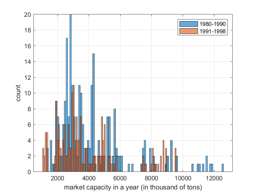
Figure 1: Histogram of market capacity per year, measured in thousand of tons.

These data represent the result of the firms’ optimal entry, exit, and investment decisions in the dynamic game estimated by Ryan (2012). We follow Otsu et al. (2016) and discretize the market production capacity into 50 bins with equal intervals of 250 thousand tons each (0-250 thousand tons, 250-500 thousand tons, and so on). For each $i=1,\ldots,n=23$ and year $t=1,\ldots,19$, we use $A_{i,t}\in\mathcal{A}=\{1,\ldots,50\}$ to denote the production capacity bin. The state variable in any market is the previous period’s action, i.e.,

$$S_{i,t}~{}=~{}A_{i,t-1},$$ (19)

and so $S_{i,t}\in\mathcal{S}=\{1,\ldots,50\}$. We note that (19) implies that the state transition probabilities are homogeneous (given by $f_{i,t+1}(s^{\prime}|a,s)=1\{s^{\prime}=a\}$), and so $H_{0}$ in (1) is equivalent to the homogeneity of the conditional choice probabilities.

Following Ryan (2012) and Otsu et al. (2016), we allow the 1990 Amendments to affect the decision of the firms. We then test the homogeneity of the conditional choice probabilities for two subsets of data: before and after 1990. That is, we implement the following hypothesis tests:

$$H_{0}^{\text{before}}:\sigma_{i,t}(a|s)=\sigma(a|s)\text{ for }i=1,\ldots,23,~{}t=1,\ldots,10,$$ (20)

$$H_{0}^{\text{after}}:\sigma_{i,t}(a|s)=\sigma(a|s)\text{ for }i=1,\ldots,23,~{}t=11,\ldots,19.$$ (21)

We note that the before and after 1990 samples used to test the hypotheses in (20) and (21) have a relatively small number of time periods ($T=10$ and $T=9$ for (20) and (21), respectively) and markets (in both cases, $n=23$). In this sense, this represents an ideal scenario for our proposed test, as its validity does not rely on either one of these dimensions diverging. We also note that both of these dimensions are smaller than the support of the data, i.e., $|\mathcal{S}|=|\mathcal{A}|=50$.

Table 2 shows the results of applying our procedure to test the hypotheses in (20) and (21). Following the literature, we use the test statistics in (5). As explained in Example 3.1, these test statistics compare market-specific conditional choice probabilities with their pooled counterpart and are thus specifically designed to detect heterogeneity across markets. This objective seems appropriate for this empirical application, as Ryan (2012)’s methodology relies on the homogeneity of the data before and after the 1990 Amendments. At a significance level of $\alpha=5\%$, we do not reject the homogeneity of the conditional choice probabilities. Our tests were implemented with $K=50,000$, but our hypothesis testing decision (i.e., non-rejection for standard significance levels) remains invariant for any $K>10,000$. Using a standard desktop computer, our Julia package completed our test with $K=50,000$ in 4.8 minutes for the subsample before 1990 and 1.9 minutes for the subsample after 1990. The computation time increases linearly with $K$.

For contrast, Table 2 also shows the results of bootstrap-based test proposed by Otsu et al. (2016). As opposed to our test, their methods reject the hypothesis of homogeneity of the conditional choice probabilities in the sample prior to 1990. Since both tests rely on the same test statistic, these differences are entirely driven by the differences in the $p$-values. Table 2 reveals that our test and the one proposed by Otsu et al. (2016) can produce different conclusions. This is also clearly shown in our Monte Carlo simulations in Section 6. It is natural to inquire which hypothesis test is correct about the homogeneity of the sample before 1990. Of course, this is impossible to determine with cetainty in an empirical application. However, we consider that our Monte Carlo evidence in Section 6.2 gives relevant information on this matter. These simulations suggest that in data settings similar to those in the empirical application (i.e., with $|\mathcal{S}|$ large relative to $n$ and $T$), our test controls size adequately while the test by Otsu et al. (2016) tends to suffer from overrejection.

	Before 1990		After 1990
	$\tau_{1}(X)$	$\tau_{2}(X)$	$\tau_{1}(X)$	$\tau_{2}(X)$
Test statistic	199.48	159.43	89.44	90.58
OPT’s p-value	0.01	0.01	0.14	0.07
Our p-value	0.21	0.12	0.73	0.68

Table 2: The test statistics $\tau_{1}(X)$ and $\tau_{2}(X)$ are defined in (5). Our test is computed according to (3) with $K=50,000$. OPT refers to Otsu et al. (2016), whose results were copied from their Table 6.

6 Monte Carlo simulations

In this section, we explore the performance of our proposed test in Monte Carlo simulations. We consider two simulation designs. Our first design is based on the duopoly entry game in Pesendorfer and Schmidt-Dengler (2008, Section 7.1). Our second design is based on our empirical application in Section 5. An important distinction between the two designs is the support of the state variable. In the first design, the state variable represents the combination of two firms’ incumbency statuses and is thus naturally limited to have four points of support. In the second design, the state variable is constructed by discretizing a continuous aggregate production capacity. As a result the support of the state variable is chosen by the researcher and may be quite large.

6.1 Simulations based on a duopoly entry game

We consider the Monte Carlo design used by Otsu et al. (2016, Section 4), which follows from the duopoly entry game in Pesendorfer and Schmidt-Dengler (2008, Section 7.1). We refer to these papers for the details on the setup. The simulated data are generated by two oligopolistic firms deciding whether to enter or not into $n$ markets, and over $T$ time periods. This dynamic game has multiple equilibria, which we exploit to generate departures from the homogeneity assumption.

In each period $t=1,\dots,T$ and market $i=1,\dots,n$, there are four possible actions in this game: $A_{i,t}=1$ denotes that neither firm entered the market, $A_{i,t}=2$ denotes that only firm 2 enters, $A_{i,t}=3$ denotes that only firm 1 enters, and $A_{i,t}=4$ denotes that both firms enter. This implies that $\mathcal{A}=\{1,2,3,4\}$. As in the empirical application, the state variable in any market is the previous period’s action (i.e., (19) holds). This implies that $\mathcal{S}=\{1,2,3,4\}$ and that the state transition probabilities are homogeneous (given by $f_{i,t+1}(s^{\prime}|a,s)~{}=~{}1\{s^{\prime}=a\}$). As a consequence, $H_{0}$ in (1) is equivalent to

$$H_{0}:\sigma_{i,t}(a|s)=\sigma(a|s).$$ (22)

The data produced by this game is a matrix $X=(S,A)\in\mathcal{X}$ constructed exactly as in Otsu et al. (2016, Section 4). We simulate data from a mixture of two data generating processes: DGP 1 and DGP 2. They represents Markov perfect equilibria of the dynamic game, which differ in the conditional choice probabilities $\sigma(a|s)$. The matrices of conditional choice probabilities in DGP 1 and DGP 2 are

$$\left(\begin{array}[]{cccc}0.19&0.30&0.12&0.18\\ 0.08&0.09&0.08&0.07\\ 0.53&0.48&0.46&0.53\\ 0.20&0.13&0.34&0.22\\ \end{array}\right)~{}~{}~{}\text{and}~{}~{}~{}\left(\begin{array}[]{cccc}0.18&0.48&0.03&0.16\\ 0.20&0.21&0.14&0.23\\ 0.29&0.22&0.13&0.26\\ 0.33&0.09&0.70&0.35\\ \end{array}\right),$$

respectively, where the columns index the value of the state $s\in\mathcal{S}=\{1,2,3,4\}$, and the rows index the value of the action $a\in\mathcal{A}=\{1,2,3,4\}$. Each market is sampled independently. Market $i=1,\dots,n$ behaves according to DGP 1 with probability $\lambda$ and DGP 2 with probability $1-\lambda$. Therefore, $\lambda\in[0,1]$ represents the average proportion of markets in DGP 1. Each market is initialized with state equal to $1$, and we simulate the corresponding action according to the conditional choice probabilities. This, in turn, determines the next period’s state according to (19), i.e., $S_{i,t+1}=A_{i,t}$. We then proceed iteratively until we have simulated $T+100$ periods for each market. The first 100 periods are discarded, producing a sample of $T$ periods for $n$ markets, which are then observed by the researcher.

For each simulated data, we implement our proposed test in (3) with $K=20,000$. We consider simulations with $n\in\{20,40,80,160\}$, $T\in\{5,10,20,40,80\}$, and $\lambda\in\{1,0,0.5,0.9\}$. As explained earlier, $\lambda$ represents the proportion of markets that are in DGP 1. If $\lambda=1$ or $\lambda=0$, all markets are sampled from the same distribution, and so the conditional choice probabilities are homogeneous across markets, i.e., $H_{0}$ holds. In turn, if $\lambda=0.5$ or $\lambda=0.9$, each data is composed of markets from both distributions, and so the conditional choice probabilities are not homogeneous across markets, i.e., $H_{0}$ fails to hold. Note that $\lambda=0.5$ generates data in which both distributions are equally represented, and so the heterogeneity in the conditional choice probabilities is more salient. On the other hand, the case with $\lambda=0.9$ produces data with a vast majority of markets in DGP 1, and so the heterogeneity in the conditional choice probabilities is harder to detect. For each simulation design, we compute rejection rates based on $2,000$ independently simulated datasets.

The results from the Monte Carlo simulation are shown in Table 3 for $\lambda\in\{0,1\}$ and Table 4 for $\lambda\in\{0.5,0.9\}$, respectively. For the sake of comparison, we also include the results from the test proposed by Otsu et al. (2016). Their test compares the same test statistics in (5) with critical values based on the bootstrap. As mentioned earlier, they show the validity of their test in an asymptotic framework with $T\to\infty$ and $n$ fixed. In contrast, our main result in Theorem 4.1 is valid for any finite $n$ and $T$.

Table 3 reveals that our test achieves relatively good size control for all values of time periods and market sizes under consideration. The table shows the result of running 80 hypothesis tests for different data configurations that satisfy $H_{0}$ (four market sizes, five time periods, two test statistics, and two distributions). Across these 80 numbers, our proposed test has an average rejection rate of 5.1%, with a standard deviation of 0.04%, and a range of 4.1% to 6.35%. We note that Theorem 4.1 implies that our test should not produce overrejection as $K$ becomes large, but it is silent about the possibility of underrejection. Table 3 reveals that our test does not seem to suffer from underrejection in these simulations. For Otsu et al. (2016)’s test, the average rejection rate is 5.1%, with a standard deviation is 2.2%, and a range of 0.6% to 13.5%. We note that the larger rejection rates occur in simulations with $T=5$, which is reasonable for a test whose validity is proven in an asymptotic framework in which $T$ diverges.

$n$	$T$	DGP 1 ($\lambda=1$)				DGP 2 ($\lambda=0$)
		Our test		OPT’s test		Our test		OPT’s test
		$\tau_{1}(X)$	$\tau_{2}(X)$	$\tau_{1}(X)$	$\tau_{2}(X)$	$\tau_{1}(X)$	$\tau_{2}(X)$	$\tau_{1}(X)$	$\tau_{2}(X)$
20	5	5.0	5.0	13.2	5.9	5.0	4.8	13.5	12.7
20	10	4.8	4.8	7.0	4.5	5.1	5.2	7.9	8.4
20	20	5.1	4.9	4.4	5.0	5.0	5.1	5.8	7.1
20	40	4.7	4.7	5.1	6.2	6.0	5.0	4.8	5.4
20	80	4.9	4.3	5.7	6.6	4.3	4.6	5.1	5.2
40	5	5.4	5.0	6.5	2.3	4.7	4.8	8.0	6.4
40	10	5.2	4.8	3.8	2.7	4.1	4.8	5.2	4.9
40	20	5.1	5.2	4.3	3.4	5.6	5.9	6.2	6.9
40	40	5.6	6.4	4.5	5.3	6.1	5.7	3.9	5.3
40	80	4.5	4.6	5.3	5.3	5.0	5.2	5.6	4.5
80	5	5.8	5.2	5.3	1.5	5.0	5.0	4.6	3.7
80	10	5.3	4.8	3.2	1.2	4.4	4.7	5.6	5.1
80	20	4.4	4.4	5.2	3.5	5.0	4.8	4.9	5.7
80	40	5.2	5.8	3.9	3.9	5.6	5.4	4.7	5.1
80	80	5.0	5.0	4.7	4.6	5.1	4.9	5.3	5.0
160	5	5.9	5.4	4.9	0.6	5.1	4.4	4.0	1.4
160	10	5.3	4.6	3.4	0.9	5.5	5.0	4.7	3.9
160	20	5.1	5.4	3.3	2.4	5.3	5.4	4.5	4.5
160	40	4.8	5.1	4.8	4.8	5.4	5.2	6.3	5.5
160	80	5.6	5.6	4.5	4.6	4.8	5.4	5.5	5.2

Table 3: Rejection rates of simulations under $H_{0}$ for $\alpha=5\%$ based on 2,000 i.i.d. simulation draws. The results for $\lambda=1$ corresponds to data sampled from DGP 1 and $\lambda=0$ corresponds to data sampled from DGP 2. The test statistics $\tau_{1}(X)$ and $\tau_{2}(X)$ are defined in (5). Our test is computed according to (3) with $K=20,000$. OPT refers to Otsu et al. (2016), whose results were copied from Tables 1 and 2 in their paper.

$n$	$T$	Mixture with $\lambda=0.5$				Mixture with $\lambda=0.9$
		Our test		OPT’s test		Our test		OPT’s test
		$\tau_{1}(X)$	$\tau_{2}(X)$	$\tau_{1}(X)$	$\tau_{2}(X)$	$\tau_{1}(X)$	$\tau_{2}(X)$	$\tau_{1}(X)$	$\tau_{2}(X)$
20	5	4.9	7.3	10.3	8.3	5.2	6.0	10.7	6.0
20	10	9.8	15.0	6.5	7.4	6.6	7.1	6.5	4.8
20	20	42.8	53.1	27.8	27.4	14.2	16.8	11.7	12.8
20	40	96.0	97.4	79.7	76.1	38.4	42.1	32.7	35.3
20	80	100	100	99.9	99.8	70.6	70.7	75.8	76.5
40	5	4.4	7.8	4.7	4.1	5.4	5.8	4.5	2.5
40	10	12.6	22.4	7.4	5.5	8.4	9.8	5.4	4.2
40	20	69.0	80.5	44.6	36.2	20.8	24.8	16.0	14.8
40	40	100	100	97.4	94.3	57.5	61.3	49.0	50.1
40	80	100	100	100	100	88.8	88.8	93.5	92.5
80	5	4.9	10.4	3.3	2.3	5.5	6.6	3.4	1.7
80	10	20.2	35.3	10.8	5.8	9.4	11.4	5.9	3.2
80	20	91.5	97.1	68.5	55.5	31.4	37.4	23.3	19.7
80	40	100	100	100	99.9	80.2	83.5	72.8	73.2
80	80	100	100	100	100	98.5	98.4	99.7	99.6
160	5	4.6	12.1	2.9	0.9	5.4	7.1	4.0	0.9
160	10	32.9	57.6	12.4	5.8	12.6	14.8	6.0	2.1
160	20	99.5	100	92.3	78.6	48.7	57.2	38.2	30.6
160	40	100	100	100	100	95.8	96.5	93.4	92.4
160	80	100	100	100	100	100	100	100	100

Table 4: Rejection rates of simulations under $H_{1}$ for $\alpha=5\%$ based on 2,000 i.i.d. simulation draws. The results for $\lambda=0.5$ corresponds to data sampled from DGP 1 and DGP 2 in equal proportions, and the results for $\lambda=0.9$ corresponds to data sampled from DGP 1 and DGP 2 with proportions 0.9 and 0.1, respectively. The test statistics $\tau_{1}(X)$ and $\tau_{2}(X)$ are defined in (5). Our test is computed according to (3) with $K=20,000$. OPT refers to Otsu et al. (2016), whose results were copied from Tables 1 and 2 in their paper.

Table 4 explores the performance of these tests for data configurations that do not satisfy $H_{0}$ due to the multiplicity of equilibria. We begin by explaining the results of the table that are common to both hypothesis tests. First, recall that $\lambda$ denotes the proportion of the $n$ markets in the data that are in DGP 1. As $\lambda$ becomes closer to either zero or one, the data are increasingly coming from a single distribution, making the departure from the $H_{0}$ harder to detect. Second, as the number of markets $n$ grows, the inference methods gain more evidence of the presence of multiplicity, resulting in higher rejection rates. The same phenomenon occurs as the number of time periods $T$ increases. Third, we find that the hypothesis tests implemented with $\tau_{2}(X)$ tend to produce higher rejection rates than those implemented with $\tau_{1}(X)$. This finding appears consistent with the large $T$ optimality result in Otsu et al. (2016, Proposition 2). We now turn to compare rejection rates between the two tests. In most simulation designs, our test appears to have a higher or equal rejection rate than Otsu et al. (2016)’s test. The few exceptions occur in designs with $n=20$ and $T\in\{5,10\}$, which correspond to designs in which Otsu et al. (2016)’s test overrejects under $H_{0}$. In other words, their power advantage relative to our test may vanish if we consider a size-corrected version of their test.

6.2 Simulations based on our empirical application

We now consider a Monte Carlo simulation design that mimics the data structure of the empirical application in Section 5. In the empirical application, we have panel data with $T=19$ periods and $n=23$ markets, and we construct the state variable by discretizing a continuous market capacity into $|\mathcal{S}|=50$ bins. Our goal in this section is to evaluate the performance of our test when the support of the data is comparable to that of the empirical application. To this end, we simulate data with $T=19$ periods, $n=23$ markets, and $|\mathcal{S}|\in\{20,35,50,65,80\}$ bins.

We simulate the data using two data-generating processes: DGP 1 and DGP 2. The first data-generating process satisfies $H_{0}$ in (1) and the second one does not. DGP 1 represents a discretized version of the pre-1990 Amendments data in the empirical application (i.e., $t\leq T_{0}\equiv 9$), and is generated as follows. First, we discretize the data into $|\mathcal{S}|$ evenly spaced bins, which we denote by $\{\tilde{S}_{i,t}:i=1,\dots,n,~{}t=1,\dots,T\}$. As in the empirical application, the state variable in any market is the previous period’s action (i.e., (19) holds). For each $i=1,\dots,n$, we simulate $S_{i,1}$ independently from the pre-1990 Amendments discretized distribution, i.e., for all $s\in\mathcal{S}=\{1,\dots,|\mathcal{S}|\}$,

$$P(S_{i,1}=s)~{}=~{}\frac{\sum_{i=1}^{n}\sum_{t=1}^{T_{0}}1\{\tilde{S}_{i,t}=s\}}{nT_{0}}.$$

Second, for each $i=1,\dots,n$ and $t=1,\dots,T-1$, we simulate $A_{i,t}$ independently across markets according to the pre-1990 Amendments choice probabilities, i.e., for all $s,a\in\mathcal{S}=\{1,\dots,|\mathcal{S}|\}$,

$$P(A_{i,t}=a|S_{i,t}=s)~{}=~{}\frac{\sum_{i=1}^{n}\sum_{t=1}^{T_{0}}1\{\tilde{S}_{i,t}=s,\tilde{A}_{i,t}=a\}}{\sum_{i=1}^{n}\sum_{t=1}^{T_{0}}1\{\tilde{S}_{i,t}=s\}},$$ (23)

where $S_{i,t}~{}=~{}A_{i,t-1}$ for all $i=1,\dots,n$ and $t=2,\dots,T$. Since the production capacity in each market and time period is drawn according to the market- and time-homogeneous conditional choice probabilities in (23), DGP 1 satisfies $H_{0}$.

DGP 2 represents an economy in which half of the markets are negatively impacted by the 1990 Amendments, and is generated as follows. For the pre-Amendments periods (i.e., $t\leq T_{0}\equiv 9$), DGP 2 coincides exactly with DGP 1. For the post-Amendments periods (i.e., $t>T_{0}$), the data is independently generated across markets in the following fashion. For markets with even index $i$ (i.e., $i=2,4,\dots,22$), the production level is distributed as in the pre-1990 Amendments periods (i.e., as in (23)). In words, markets with even index $i$ are not affected by the 1990 Amendments. For markets with odd index $i$ (i.e., $i=1,3,\dots,23$), the production level is uniformly chosen to be weakly lower, i.e., for all $s,a\in\mathcal{S}=\{1,\dots,|\mathcal{S}|\}$,

$$P(A_{i,t}=a|S_{i,t}=s)~{}=~{}\frac{1\{a\leq s\}}{s}.$$

In words, markets with odd index $i$ are negatively affected by the 1990 Amendments. As in DGP 1, the state variable in any market is the previous period’s action (i.e., (19) holds). The structural change caused by the 1990 Amendments implies that DGP 2 does not satisfy $H_{0}$.

For each simulated data, we implement our proposed test in (3) with $K=20,000$. As mentioned earlier, we consider simulations with $n=23$, $T=19$, $T_{0}=9$, and $|\mathcal{S}|\in\{20,35,50,65,80\}$. The first three parameters are those in the empirical application, which uses $|\mathcal{S}|=50$ bins. For each simulation design, we compute rejection rates based on $2,000$ independently simulated datasets.

The results from the Monte Carlo simulations are presented in Table 5. We include results for our test and the one proposed by Otsu et al. (2016) with bootstrap-based $p$-values (see their Section 5 for details). We first describe results under DGP 1, i.e., when $H_{0}$ holds. Our test achieves good size control for all discretizations under consideration. Across the 10 hypothesis tests that satisfy $H_{0}$ (five discretizations and two test statistics), our test has an average rejection rate of 5.4%, a standard deviation of 0.3%, and a range of 4.9% to 5.9%. These numbers also reveal that our test does not exhibit underrejection. On the other hand, Otsu et al. (2016)’s test suffers from overrejection, and this problem tends to exacerbate as $|\mathcal{S}|$ increases. For instance, when $|\mathcal{S}|$ is as in the empirical application (i.e., $|\mathcal{S}|=50$), their test has a rejection rate of 23.1% for $\tau_{1}(X)$ and 26% for $\tau_{2}(X)$, more than 4 times higher than the nominal size of $\alpha=5\%$. This issue may be explained by the fact that their validity result relies on $T\to\infty$, and these simulations only have $T=19$, which is smaller than $|\mathcal{S}|\in\{20,35,50,65,80\}$.

We now turn to the simulations under DGP 2, i.e., when $H_{0}$ fails to hold. The results show that our test has nontrivial power for all values of $|\mathcal{S}|\in\{20,35,50,65,80\}$. If particular, when $|\mathcal{S}|$ is as in the empirical application (i.e., $|\mathcal{S}|=50$), our test has a rejection rate of 36% for $\tau_{1}(X)$ and 21.6% for $\tau_{2}(X)$, which are considerably larger than the nominal size of $\alpha=5\%$. As one may expect, the power of our test tends to decrease with $|\mathcal{S}|$. This is because the power of our test is based on “relevant” data permutations, which become increasingly rare as $|\mathcal{S}|$ grows. Also noteworthy is that, for $|\mathcal{S}|>20$, our test implemented with $\tau_{1}(X)$ has more power than when implemented with $\tau_{2}(X)$, which is an opposite pattern to that in the previous Monte Carlo simulations. Finally, we recognize that Otsu et al. (2016)’s test achieves much higher rejection rates, but these occur in the context of overrejection under the null hypothesis.

	DGP 1 (i.e., $H_{0}$ holds)				DGP 2 (i.e., $H_{0}$ fails)
	Our test		OPT’s test		Our test		OPT’s test
$|\mathcal{S}|$	$\tau_{1}(X)$	$\tau_{2}(X)$	$\tau_{1}(X)$	$\tau_{2}(X)$	$\tau_{1}(X)$	$\tau_{2}(X)$	$\tau_{1}(X)$	$\tau_{2}(X)$
20	5.3	5.9	17.0	15.9	36.0	50.7	94.0	98.5
35	5.2	5.1	24.0	29.0	34.0	24.8	99.6	100
50	5.6	5.8	23.1	26.0	36.0	21.6	99.8	100
65	5.6	5.3	56.4	69.8	29.8	20.8	100	100
80	5.4	4.9	48.4	64.8	30.8	18.1	100	100

Table 5: Simulation results under DGP 1 (i.e., $H_{0}$ holds) and DGP 2 (i.e., $H_{0}$ fails). The test statistics $\tau_{1}(X)$ and $\tau_{2}(X)$ are defined in (5). Our test is computed according to (3) with $K=20,000$. OPT refers to Otsu et al. (2016), whose results were generated by the bootstrap method described in their Section 5.

7 Conclusions

This paper proposes a hypothesis test for the “homogeneity assumption” in dynamic discrete games. Our test is implemented by an MCMC algorithm and does not rely on functional forms imposed by the researcher. We show that our test is valid as the (user-defined) number of MCMC draws diverges, regardless of the number of markets and time periods in the data. This result contrasts with that of available methods in the literature, which require the number of time periods to diverge. We establish our validity result by showing that our proposed test is an MCMC approximation to a computationally infeasible underlying randomization test, which is valid in finite samples. Our Monte Carlo simulations confirm that our test has an excellent performance in finite samples, both in terms of size control and power.

Appendix A Appendix to Section 3

To save on notation, this appendix treats ordered pairs such as $I=(I_{1},I_{2})$ and $I^{(k)}=(I_{1},I_{2})$ as the set $\{I_{1},I_{2}\}$ whenever this does not generate confusion.

A.1 Implementation of Step 2 in our MCMC algorithm

For any $k=2,\ldots,K$, $S^{(k-1)}\in\mathcal{S}^{nT}$, and $I^{(k)}$ selected in Step 1 of our MCMC algorithm, Step 2 of our MCMC algorithm draws $S^{(k)}$ uniformly within $R_{S}(I^{(k)},S^{(k-1)})$. To implement this step, we propose a modification of the Euler Algorithm. For a description of the Euler Algorithm, see Kandel et al. (1996); Besag and Mondal (2013). We first describe the original Euler Algorithm in Algorithm A.1 and then introduce our modification in Algorithm A.2. Throughout this section, we use $0$ to represent an auxiliary value for the state variable that does not belong to the observed values of the state variable, as $0\not\in\mathcal{S}=\{1,2,\dots,|\mathcal{S}|\}$.

Algorithm A.1 (Euler Algorithm).

Given a sequence $\breve{\xi}\in(\mathcal{S}\cup\{0\})^{V}$ with $V\equiv dim(\breve{\xi})\geq 2$, this algorithm randomly generates a sequence $\tilde{\xi}=(\tilde{\xi}_{1},\ldots,\tilde{\xi}_{V})$ in the following fashion:

• Step 1: For every $s,s^{\prime}\in\mathcal{S}\cup\{0\}$, set

  $$N^{(0)}(s,s^{\prime})~{}=~{}1\{(\breve{\xi}_{V},\breve{\xi}_{1})=(s,s^{\prime})\}+\sum_{v=1}^{V-1}1\{(\breve{\xi}_{v},\breve{\xi}_{v+1})=(s,s^{\prime})\}.$$ (A-1)

  Also, set $\zeta_{1}=\breve{\xi}_{V}$ and $v=1$. Then, do the following:

  1. Given $\zeta_{v}$, generate $\zeta_{v+1}$ according to the following distribution:

     $$P(\zeta_{v+1}=s\mid\zeta_{v})~{}=~{}\frac{N^{(0)}(s,\zeta_{v})}{\sum_{s^{\prime}\in\mathcal{S}\cup\{0\}}N^{(0)}(s^{\prime},\zeta_{v})},$$ (A-2)

     where $\sum_{s\in\mathcal{S}\cup\{0\}}N^{(0)}(s,\zeta_{v})\geq 1$ is guaranteed by Step 1.

  2. If $(\zeta_{2},\ldots,\zeta_{v+1})$ does not exhaust all the values in $\breve{\xi}$, then increase $v$ by one and go back to (a). Otherwise, set $\bar{v}=v+1$ and go to Step 2.

• Step 2: Set ${\tilde{\xi}}_{1}=\breve{\xi}_{1}$. Also, for every $s,s^{\prime}\in\mathcal{S}\cup\{0\}$, set

  $$N^{(1)}(s,s^{\prime})~{}=~{}\sum_{v=1}^{V-1}1\{(\breve{\xi}_{v},\breve{\xi}_{v+1})=(s,s^{\prime})\}-1\{s^{\prime}=\zeta_{(\min\{v=2,\ldots,\bar{v}:\ \zeta_{v}=s\}-1)},s\neq\breve{\xi}_{V}\}.$$ (A-3)

  For $v=2,\ldots,V$, repeat the following:

  • Given $\tilde{\xi}_{v-1}$, generate $\tilde{\xi}_{v}$ according to

    $$P(\tilde{\xi}_{v}=s^{\prime}\mid\tilde{\xi}_{v-1}=s)~{}=~{}\left\{\begin{array}[]{cc}\dfrac{N^{(v-1)}(s,s^{\prime})}{\sum_{s^{\prime\prime}\in\mathcal{S}\cup\{0\}}N^{(v-1)}(s,s^{\prime\prime})}&\text{ if }\sum_{s^{\prime\prime}\in\mathcal{S}\cup\{0\}}N^{(v-1)}(s,s^{\prime\prime})\geq 1,\\ 1\{s^{\prime}=\zeta_{(\min\{v=2,\ldots,\bar{v}:\ \zeta_{v}=s\}-1)}\}&\text{ otherwise}.\end{array}\right.$$ (A-6)

  • For every $s,s^{\prime}\in\mathcal{S}\cup\{0\}$, set $N^{(v)}(s,s^{\prime})~{}=~{}N^{(v-1)}(s,s^{\prime})-1\{N^{(v-1)}(s,s^{\prime})>0,(\tilde{\xi}_{v-1},\tilde{\xi}_{v})=(s,s^{\prime})\}$ for every $s,s^{\prime}\in\mathcal{S}\cup\{0\}$.

Example A.1 (Applying the Euler Algorithm in a simple case).

For the sake of illustration, we now apply the Euler Algorithm A.1 to the sequence $\breve{\xi}=(1,1,2,1,2)$. This sequence was chosen because it is an application of the Euler Algorithm that is both simple to explain and non-trivial. Note that $\breve{\xi}$ has $\dim(\breve{\xi})=V=5$ and only two values: 1 and 2. Also, $(0\cup\mathcal{S})=\{0,1,2\}$. As we now demonstrate, the Euler Algorithm applied to $\breve{\xi}$ produces a new sequence $\tilde{\xi}$ that is uniformly distributed in the set $\{(1,1,2,1,2),(1,2,1,1,2)\}$.

• Step 1: We start by definiting $N^{(0)}(s,s^{\prime})$ for $s,s^{\prime}\in\{0,1,2\}$. Following (A-1), $N^{(0)}(s,s^{\prime})=0$ if $s=0$ or $s^{\prime}=0$, $N^{(0)}(1,1)=1$, $N^{(0)}(1,2)=2$, $N^{(0)}(2,1)=2$, and $N^{(0)}(2,2)=0$. Also, we set $\zeta_{1}=\breve{\xi}_{5}=2$ and $v=1$.

  Next, consider (a). This generates $\zeta_{2}$ according to (A-2), i.e.,

  $$P(\zeta_{2}=s|\zeta_{1}=2)=\frac{N^{(0)}(s,2)}{N^{(0)}(0,2)+N^{(0)}(1,2)+N^{(0)}(2,2)}=1\{s=1\},$$

  and so $\zeta_{2}=1$.

  We next consider (b). In this case, note that $\zeta_{2}=1$ does not include all the values in $\breve{\xi}=(1,1,2,1,2)$, i.e., 1 and 2. Thus, we increase $v$ by one, i.e., $v=2$, and return to (a).

  In the new instance of (a), we generate $\zeta_{3}$ according to (A-2), i.e.,

  $$P(\zeta_{3}=s|\zeta_{2}=1)=\frac{N^{(0)}(s,1)}{N^{(0)}(0,1)+N^{(0)}(1,1)+N^{(0)}(2,1)}=\frac{1\{s=1\}+2\times 1\{s=2\}}{3}.$$

  That is, $\zeta_{3}=1$ with probability $1/3$ and $\zeta_{3}=2$ with probability $2/3$. If $\zeta_{3}=1$ occurs, then $(\zeta_{2},\zeta_{3})=(1,1)$ does not include 1 and 2. Thus, we increase $v$ by one, i.e., $v=2$, and we return to (a). In turn, if $\zeta_{3}=2$ occurs, then $(\zeta_{2},\zeta_{3})=(1,2)$ includes 1 and 2, and we move on to step 3.

  By construction, the repetition of (a)-(b) will continue until $(\zeta_{2},\ldots,\zeta_{v+1})$ includes all the values in $\breve{\xi}=(1,1,2,1,2)$, i.e., 1 and 2. As a result of this, Step 1 of the Euler Algorithm generates $\zeta=(2,1,1,\ldots,1,2)$, where the length of the 1’s in the middle of $\zeta$ denotes the number of times (a)-(b) have been repeated. By definition, $\bar{v}$ is the length of $\zeta$. Finally, it is relevant for step 2 that $\min\{v=2,\ldots,\bar{v}:~{}\zeta_{v}=1\}=2$ and $\min\{v=2,\ldots,\bar{v}:~{}\zeta_{v}=2\}=\bar{v}$.

• Step 2: Set ${\tilde{\xi}}_{1}=\breve{\xi}_{1}=1$. Also, we set $N^{(0)}(s,s^{\prime})$ for $s,s^{\prime}\in\{0,1,2\}$. Following (A-3), $N^{(1)}(1,s^{\prime})=1$ and $N^{(1)}(2,s^{\prime})=2\times 1\{s^{\prime}=1\}$. Then, we move on to (a).

  In (a), we then generate $\tilde{\xi}_{2}$ according to (A-6), i.e.,

  $$P(\tilde{\xi}_{2}=s^{\prime}|\tilde{\xi}_{1}=s)=\frac{N^{(1)}(1,s^{\prime})}{N^{(1)}(1,0)+N^{(1)}(1,1)+N^{(1)}(1,2)}=\frac{1\{s^{\prime}\in\{1,2\}\}}{2}.$$

  That is, the algorithm chooses $\tilde{\xi}_{2}$ equal to $1$ or $2$ with equal probability. We now divide the argument into two cases.

  • Case 1: $\tilde{\xi}_{2}=1$. Then, (b) sets $N^{(2)}(1,s^{\prime})=1\{s^{\prime}=2\}$ and $N^{(2)}(2,s^{\prime})=2\times 1\{s^{\prime}=1\}$. Then, (a) generates $\tilde{\xi}_{3}$ according to (A-6). Since $\tilde{\xi}_{2}=1$ and $\sum_{s^{\prime\prime}\in\{0,1,2\}}N^{(2)}(1,s^{\prime\prime})=1$, this gives

    $$P(\tilde{\xi}_{3}=s^{\prime}|\tilde{\xi}_{2}=1)=\frac{N^{(2)}(1,s^{\prime})}{N^{(2)}(1,0)+N^{(2)}(1,1)+N^{(2)}(1,2)}=1\{s^{\prime}=2\},$$

    and so $\tilde{\xi}_{3}=2$. Then, (b) sets $N^{(3)}(1,s^{\prime})=0$ and $N^{(3)}(2,s^{\prime})=2\times 1\{s^{\prime}=1\}$. Then, (a) generates $\tilde{\xi}_{4}$ according to (A-6). Since $\tilde{\xi}_{3}=2$ and $\sum_{s^{\prime\prime}\in\{0,1,2\}}N^{(3)}(2,s^{\prime\prime})=2$, this gives

    $$P(\tilde{\xi}_{4}=s^{\prime}|\tilde{\xi}_{3}=2)=\frac{N^{(3)}(2,s^{\prime})}{N^{(3)}(2,0)+N^{(3)}(2,1)+N^{(3)}(2,2)}=1\{s^{\prime}=1\},$$

    and so $\tilde{\xi}_{4}=1$. Then, (b) sets $N^{(4)}(1,s^{\prime})=0$ and $N^{(4)}(2,s^{\prime})=1\{s^{\prime}=1\}$. Then, (a) generates $\tilde{\xi}_{5}$ according to (A-6). Since $\tilde{\xi}_{4}=1$ and $\sum_{s^{\prime\prime}\in\{0,1,2\}}N^{(4)}(1,s^{\prime\prime})=0$, this gives

    $$P(\tilde{\xi}_{5}=s^{\prime}|\tilde{\xi}_{4}=1)=1\{s^{\prime}=\zeta_{(\min\{v=2,\ldots,\bar{v}:~{}\zeta_{v}=1\}-1)}\}=1\{s^{\prime}=2\},$$

    and so $\tilde{\xi}_{5}=2$, where we have used that $\min\{v=2,\ldots,\bar{v}:~{}\zeta_{v}=1\}=2$. In conclusion, the resulting sequence is $\tilde{\xi}=(1,1,2,1,2)$.

  • Case 2: $\tilde{\xi}_{2}=2$. By repeating the arguments in case 1, it is not hard to see that the resulting sequence in case 2 is $\tilde{\xi}=(1,2,1,1,2)$.

Since Case 1 (i.e., $\tilde{\xi}_{2}=1$) and Case 2 (i.e., $\tilde{\xi}_{2}=2$) in step 2 are equally likely, we conclude that the Euler Algorithm generates the sequences $\tilde{\xi}=(1,1,2,1,2)$ and $\tilde{\xi}=(1,2,1,1,2)$ with equal probability, as desired.   

Before we describe the central property of the Euler Algorithm, we first introduce the following definition.

Definition A.1.

For any $\breve{\xi}\in(\mathcal{S}\cup\{0\})^{V}$, let $R_{S0}(\breve{\xi})$ denote the set of all $\tilde{\xi}\in(\mathcal{S}\cup\{0\})^{V}$ that satisfy the following conditions:

1. $\tilde{\xi}_{1}=\breve{\xi}_{1}$,

2. $\sum_{v=1}^{V-1}1\{\tilde{\xi}_{v}=s,\tilde{\xi}_{v+1}=s^{\prime}\}=\sum_{v=1}^{V-1}1\{\breve{\xi}_{v}=s,\breve{\xi}_{v+1}=s^{\prime}\}$ for all $s,s^{\prime}\in\mathcal{S}\cup\{0\}$.

Note that $\breve{\xi}\in R_{S0}(\breve{\xi})$, and so $R_{S0}(\breve{\xi})\neq\emptyset$. Next, we give the main property of the Euler Algorithm.

Lemma A.1.

For any $\breve{\xi}\in(\mathcal{S}\cup\{0\})^{V}$, the outcome of the Euler Algorithm given $\breve{\xi}$ (i.e., Algorithm A.1) is uniformly distributed over $R_{S0}(\breve{\xi})$ conditional on $\breve{\xi}$.

Proof.

See Kandel et al. (1996, Theorem 2).  

We now introduce our modification of the Euler Algorithm to construct $S^{(k)}$ for any $k=2,\ldots,K$.

Algorithm A.2 (Generation of $S^{(k)}$).

For any $k=2,\ldots,K$ and given $(X^{(1)},\ldots,X^{(k-1)},I^{(k)})$, $S^{(k)}$ is randomly generated as follows:

• Case 1: $I_{1}^{(k)}\neq I_{2}^{(k)}$.

  • Step 1: Set $\xi^{(k-1)}=(S_{I_{1}^{(k)},1}^{(k-1)},\ldots,S_{I_{1}^{(k)},T}^{(k-1)},0,S_{I_{2}^{(k)},1}^{(k-1)},\ldots,S_{I_{2}^{(k)},T}^{(k-1)},0).$

  • Step 2: Generate $\xi^{(k)}$ as follows:

    • Generate a random draw of ${\xi}$ using the Euler Algorithm given $\xi^{(k-1)}$.

    • If ${\xi}_{T+1}=0$, set $\xi^{(k)}=\xi$ and go to Step 3. Otherwise, return to (a).

  • Step 3: Given $\xi^{(k)}$, generate $S^{(k)}$ as follows:

    • For every $i\notin I^{(k)}$, generate $(S_{i,1}^{(k)},\ldots,S_{i,T}^{(k)})$ using the Euler Algorithm given $(S_{i,1}^{(k-1)},\ldots,S_{i,T}^{(k-1)})$.

    • $(S_{I_{1}^{(k)},1}^{(k)},\ldots,S_{I_{1}^{(k)},T}^{(k)})=(\xi^{(k)}_{1},\dots,\xi^{(k)}_{T})$.

    • $(S_{I_{2}^{(k)},1}^{(k)},\ldots,S_{I_{2}^{(k)},T}^{(k)})=(\xi^{(k)}_{T+2},\dots,\xi^{(k)}_{2T+1})$.

• Case 2: $I_{1}^{(k)}=I_{2}^{(k)}$. For every $i=1,\ldots,n$, generate $(S_{i,1}^{(k)},\ldots,S_{i,T}^{(k)})$ using the Euler Algorithm given $(S_{i,1}^{(k-1)},\ldots,S_{i,T}^{(k-1)})$. $\blacksquare$

Lemma A.2 shows that $S^{(k)}$ generated by Algorithm A.2 has the desired properties.

Lemma A.2.

For any $k=2,\ldots,K$, $S^{(k)}$ generated by Algorithm A.2 satisfies the requirements of Step 2 of our MCMC algorithm, i.e., (8) holds.

Proof.

We fix $k=2,\ldots,K$, $(X^{(1)},\ldots,X^{(k-1)})$, and a generic $\breve{S}\in\mathcal{S}^{nT}$ arbitrarily throughout this proof. We divide the proof in two cases.

Case 1: $I_{1}^{(k)}\not=I_{2}^{(k)}$. For $S^{(k-1)}$ and $S^{(k)}$ determined by $X^{(k-1)}=(S^{(k-1)},A^{(k-1)})$ and $X^{(k)}=(S^{(k)},A^{(k)})$, and for a generic $\breve{S}\in\mathcal{S}^{nT}$, we set

$${\xi}^{(k-1)} =({S}_{I_{1}^{(k-1)},1},\ldots,{S}_{I_{1}^{(k-1)},T},0,{S}_{I_{2}^{(k-1)},1},\ldots,{S}_{I_{2}^{(k-1)},T},0),$$

$${\xi}^{(k)} =({S}_{I_{1}^{(k)},1},\ldots,{S}_{I_{1}^{(k)},T},0,{S}_{I_{2}^{(k)},1},\ldots,{S}_{I_{2}^{(k)},T},0),$$

$$\breve{\xi} =(\breve{S}_{I_{1}^{(k)},1},\ldots,\breve{S}_{I_{1}^{(k)},T},0,\breve{S}_{I_{2}^{(k)},1},\ldots,\breve{S}_{I_{2}^{(k)},T},0).$$

Step 3 of Algorithm A.2 implies

$$P(S^{(k)}=\breve{S}\mid I^{(k)},X^{(1)},\ldots,X^{(k-1)})=$$

$$\left\{\begin{array}[]{c}P(\xi^{(k)}=\breve{\xi}\mid{\xi}^{(k-1)})\times\\ \prod_{i\not\in I^{(k)}}P((S_{i,1}^{(k)},\ldots,S_{i,T}^{(k)})=(\breve{S}_{i,1},\ldots,\breve{S}_{i,T})\mid S_{i,1}^{(k-1)},\ldots,S_{i,T}^{(k-1)})\end{array}\right\},$$ (A-9)

Lemma A.1 implies that

$$P((S_{i,1}^{(k)},\ldots,S_{i,T}^{(k)})=(\breve{S}_{i,1},\ldots,\breve{S}_{i,T})\mid S_{i,1}^{(k-1)},\ldots,S_{i,T}^{(k-1)})=\frac{1\{(\breve{S}_{i,1},\ldots,\breve{S}_{i,T})\in R_{S0}(S_{i,1}^{(k-1)},\ldots,S_{i,T}^{(k-1)})\}}{|R_{S0}(S_{i,1}^{(k-1)},\ldots,S_{i,T}^{(k-1)})|}$$ (A-10)

for every $i\not\in I^{(k)}$. In turn, Lemma A.3 implies that

$$P(\xi^{(k)}=\breve{\xi}\mid\xi^{(k-1)})=\frac{1\{\breve{\xi}\in R_{S0}(\xi^{(k-1)}):\breve{\xi}_{T+1}=0\}}{|\{\tilde{\xi}\in R_{S0}(\xi^{(k-1)}):\tilde{\xi}_{T+1}=0\}|}.$$ (A-11)

By combining (A-9), (A-10), and (A-11),

$$P(S^{(k)}=\breve{S}\mid I^{(k)},X^{(1)},\ldots,X^{(k-1)})=$$

$$\frac{1\{\breve{\xi}\in R_{S0}(\xi^{(k-1)}):\breve{\xi}_{T+1}=0\}\times\prod_{i\not\in I^{(k)}}1\{(\breve{S}_{i,1},\ldots,\breve{S}_{i,T})\in R_{S0}(S_{i,1}^{(k-1)},\ldots,S_{i,T}^{(k-1)})\}}{|\{\tilde{\xi}\in R_{S0}(\xi^{(k-1)}):\tilde{\xi}_{T+1}=0\}|\times\prod_{i\not\in I^{(k)}}|R_{S0}(S_{i,1}^{(k-1)},\ldots,S_{i,T}^{(k-1)})|}.$$ (A-12)

To complete the proof, it suffices to show that the right-hand side of (A-12) is equal to the right-hand side of (8). To this end, it suffices to show that

$$1\{\breve{\xi}\in R_{S0}(\xi^{(k-1)}):\breve{\xi}_{T+1}=0\}\times\prod_{i\not\in I^{(k)}}1\{(\breve{S}_{i,1},\ldots,\breve{S}_{i,T})\in R_{S0}(S_{i,1}^{(k-1)},\ldots,S_{i,T}^{(k-1)})\}$$

$$=1\{\breve{S}\in R_{S}(I^{(k)},S^{(k-1)})\}$$ (A-13)

and

$$|\{\tilde{\xi} \in R_{S0}(\xi^{(k-1)}):\tilde{\xi}_{T+1}=0\}|\times\prod_{i\not\in I^{(k)}}|R_{S0}(S_{i,1}^{(k-1)},\ldots,S_{i,T}^{(k-1)})|=|R_{S}(I^{(k)},S^{(k-1)})|.$$ (A-14)

To show (A-13), consider the following derivation.

$$1\{\breve{\xi}\in R_{S0}(\xi^{(k-1)}):\breve{\xi}_{T+1}=0\}\times\prod_{i\not\in I^{(k)}}1\{(\breve{S}_{i,1},\ldots,\breve{S}_{i,T})\in R_{S0}(S_{i,1}^{(k-1)},\ldots,S_{i,T}^{(k-1)})\}$$

$$=\left\{\begin{array}[]{c}1\{(\breve{S}_{I_{1}^{(k)},1},\ldots,\breve{S}_{I_{1}^{(k)},T},0,\breve{S}_{I_{2}^{(k)},1},\ldots,\breve{S}_{I_{2}^{(k)},T},0)\in R_{S0}(\xi^{(k-1)})\}\\ \times\prod_{i\not\in I^{(k)}}1\{(\breve{S}_{i,1},\ldots,\breve{S}_{i,T})\in R_{S0}(S_{i,1}^{(k-1)},\ldots,S_{i,T}^{(k-1)})\}\end{array}\right\}$$

$$\overset{(1)}{=}1\left\{\begin{array}[]{c}\breve{S}_{i,1}={S}_{i,1}^{(k-1)}~{}\text{for all}~{}i=1,\ldots,n,\\ \sum_{i\in I^{(k)}}\sum_{t=1}^{T-1}1\{\breve{S}_{i,t}=s,\breve{S}_{i,t+1}=s^{\prime}\}=\sum_{i\in I^{(k)}}\sum_{t=1}^{T-1}1\{S_{i,t}^{(k-1)}=s,S_{i,t+1}^{(k-1)}=s^{\prime}\}~{}\forall s,s^{\prime}\in\mathcal{S},\\ \sum_{i\in I^{(k)}}1\{\breve{S}_{i,T}=s\}=\sum_{i\in I^{(k)}}1\{S_{i,T}^{(k-1)}=s\}~{}\text{for all}~{}s\in\mathcal{S},\\ \sum_{t=1}^{T-1}1\{\breve{S}_{i,t}=s,\breve{S}_{i,t+1}=s^{\prime}\}=\sum_{t=1}^{T-1}1\{S_{i,t}^{(k-1)}=s,S_{i,t+1}^{(k-1)}=s^{\prime}\}~{}\text{for all}~{}s,s^{\prime}\in\mathcal{S},~{}i\not\in I^{(k)}\end{array}\right\}$$

$$\overset{(2)}{=}1\left\{\begin{array}[]{c}\breve{S}_{i,1}={S}_{i,1}^{(k-1)}~{}\text{for all}~{}i=1,\ldots,n,\\ \sum_{i\in I^{(k)}}\sum_{t=1}^{T-1}1\{\breve{S}_{i,t}=s,\breve{S}_{i,t+1}=s^{\prime}\}=\sum_{i\in I^{(k)}}\sum_{t=1}^{T-1}1\{S_{i,t}^{(k-1)}=s,S_{i,t+1}^{(k-1)}=s^{\prime}\}~{}\forall s,s^{\prime}\in\mathcal{S},\\ \sum_{t=1}^{T-1}1\{\breve{S}_{i,t}=s,\breve{S}_{i,t+1}=s^{\prime}\}=\sum_{t=1}^{T-1}1\{S_{i,t}^{(k-1)}=s,S_{i,t+1}^{(k-1)}=s^{\prime}\}~{}\text{for all}~{}s,s^{\prime}\in\mathcal{S},~{}i\not\in I^{(k)}\end{array}\right\}$$

$$\overset{(3)}{=}1\{\breve{S}\in R_{S}(I^{(k)},S^{(k-1)})\},$$

as desired, where (1) follows from $I_{1}^{(k)}\not=I_{2}^{(k)}$ and applying Definition A.1, (2) follows from Lemma A.4, and (3) follows from Definition 3.1. To show (A-14), consider the following argument.

$$1 =\sum_{\breve{S}\in\mathcal{S}}P(S^{(k)}=\breve{S}\mid I^{(k)},X^{(1)},\ldots,X^{(k-1)})$$

$$\overset{(1)}{=}\frac{\sum_{\breve{S}\in\mathcal{S}}1\{\breve{S}\in R_{S}(I^{(k)},S^{(k-1)})\}}{|\{\tilde{\xi}\in R_{S0}(\xi^{(k-1)}):\tilde{\xi}_{T+1}=0\}|\times\prod_{i\not\in I^{(k)}}|R_{S0}(S_{i,1}^{(k-1)},\ldots,S_{i,T}^{(k-1)})|}$$

$$=\frac{|R_{S}(I^{(k)},S^{(k-1)})|}{|\{\tilde{\xi}\in R_{S0}(\xi^{(k-1)}):\tilde{\xi}_{T+1}=0\}|\times\prod_{i\not\in I^{(k)}}|R_{S0}(S_{i,1}^{(k-1)},\ldots,S_{i,T}^{(k-1)})|},$$

where (1) follows from combining (A-12) and (A-13). From here, (A-14) follows.

Case 2: $I_{1}^{(k)}=I_{2}^{(k)}$. Algorithm A.2 implies

$$P(S^{(k)}=\breve{S}\mid I^{(k)},X^{(1)},\ldots,X^{(k-1)})=\prod_{i=1}^{n}P((S_{i,1}^{(k)},\ldots,S_{i,T}^{(k)})=(\breve{S}_{i,1},\ldots,\breve{S}_{i,T})\mid S_{i,1}^{(k-1)},\ldots,S_{i,T}^{(k-1)}).$$ (A-15)

Lemma A.1 implies that for every $i=1,\ldots,n$,

$$P((S_{i,1}^{(k)},\ldots,S_{i,T}^{(k)})=(\breve{S}_{i,1},\ldots,\breve{S}_{i,T})\mid S_{i,1}^{(k-1)},\ldots,S_{i,T}^{(k-1)})=\frac{1\{(\breve{S}_{i,1},\ldots,\breve{S}_{i,T})\in R_{S0}(S_{i,1}^{(k-1)},\ldots,S_{i,T}^{(k-1)})\}}{|R_{S0}(S_{i,1}^{(k-1)},\ldots,S_{i,T}^{(k-1)})|}.$$ (A-16)

By combining (A-15) and (A-16)

$$P(S^{(k)}=\breve{S}\mid I^{(k)},X^{(1)},\ldots,X^{(k-1)}) =\prod_{i=1}^{n}\frac{1\{(\breve{S}_{i,1},\ldots,\breve{S}_{i,T})\in R_{S0}(S_{i,1}^{(k-1)},\ldots,S_{i,T}^{(k-1)})\}}{|R_{S0}(S_{i,1}^{(k-1)},\ldots,S_{i,T}^{(k-1)})|}$$

$$=\frac{\prod_{i=1}^{n}1\{(\breve{S}_{i,1},\ldots,\breve{S}_{i,T})\in R_{S0}(S_{i,1}^{(k-1)},\ldots,S_{i,T}^{(k-1)})\}}{\prod_{i=1}^{n}|R_{S0}(S_{i,1}^{(k-1)},\ldots,S_{i,T}^{(k-1)})|}.$$ (A-17)

To complete the proof, it suffices to show that the right-hand side of (A-17) is equal to the right-hand side of (8). To this end, it suffices to show that

$$\prod_{i=1}^{n}1\{(\breve{S}_{i,1},\ldots,\breve{S}_{i,T})\in R_{S0}(S_{i,1}^{(k-1)},\ldots,S_{i,T}^{(k-1)})\} =1\{\breve{S}\in R_{S}(I^{(k)},S^{(k-1)})\}$$ (A-18)

$$\prod_{i=1}^{n}|R_{S0}(S_{i,1}^{(k-1)},\ldots,S_{i,T}^{(k-1)})| =|R_{S}(I^{(k)},S^{(k-1)})|.$$ (A-19)

To show (A-18), consider the following derivation.

$$\prod_{i=1}^{n}1\{(\breve{S}_{i,1},\ldots,\breve{S}_{i,T})\in R_{S0}(S_{i,1}^{(k-1)},\ldots,S_{i,T}^{(k-1)})\}$$

$$\overset{(1)}{=}1\left\{\begin{array}[]{c}\breve{S}_{i,1}={S}_{i,1}^{(k-1)}\text{ for all }i=1,\dots,n,\\ \sum_{t=1}^{T-1}1\{\breve{S}_{i,t}=s,\breve{S}_{i,t+1}=s^{\prime}\}=\sum_{t=1}^{T-1}1\{S_{i,t}^{(k-1)}=s,S_{i,t+1}^{(k-1)}=s^{\prime}\}\text{ for all }s,s^{\prime}\in\mathcal{S}~{}\text{and}~{}i=1,\dots,n\end{array}\right\}$$

$$\overset{(2)}{=}1\{\breve{S}\in R_{S}(I^{(k)},S^{(k-1)})\},$$

as desired, where (1) follows from $I_{1}^{(k)}=I_{2}^{(k)}$ and applying Definition A.1 for each $i=1,\ldots,n$, and (2) follows from Definition 3.1. Finally, (A-19) can be shown by using an argument that is analogous to the one used to prove (A-14). We omit this for the sake of brevity.  

Lemma A.3.

For any $k=2,\ldots,K$, if $\xi^{(k)}$ is generated by Algorithm A.2, then $\xi^{(k)}$ is uniformly distributed over the set $\{\xi\in R_{S0}(\xi^{(k-1)}):\xi_{T+1}=0)\}$ conditional on $(I^{(k)},X^{(1)},\ldots,X^{(k-1)})$.

Proof.

By Lemma A.1, $\tilde{\xi}$ in Step 2(a) of Algorithm A.2 follows the uniform distribution on $R_{S0}(\xi^{(k-1)})$, conditional on $(I^{(k)},X^{(1)},\ldots,X^{(k-1)})$. Steps 2(b) of Algorithm A.2 truncates the variable to the set $\{\xi\in R_{S0}(\xi^{(k-1)}):\xi_{T+1}=0\}$. The desired result then follows from the fact that a truncated version of a discrete uniform distribution is uniformly distributed on the truncated set.  

Lemma A.4.

For any $I\in\mathcal{I}$, if $\breve{S},\tilde{S}\in\mathcal{S}^{nT}$ satisfy the following conditions:

1. $\tilde{S}_{i,1}=\breve{S}_{i,1}$ for all $i\in I$,

2. $\sum_{i\in I}\sum_{t=1}^{T-1}1\{\tilde{S}_{i,t}=s,\tilde{S}_{i,t+1}=s^{\prime}\}=\sum_{i\in I}\sum_{t=1}^{T-1}1\{\breve{S}_{i,t}=s,\breve{S}_{i,t+1}=s^{\prime}\}$ for all $s,s^{\prime}\in\mathcal{S}$,

then, $\sum_{i\in I}1\{\tilde{S}_{i,T}=s\}=\sum_{i\in I}1\{\breve{S}_{i,T}=s\}$ for all $s\in\mathcal{S}$.

Proof.

For every $i\in I$ and $s\in\mathcal{S}$, note that

$$1\{\breve{S}_{i,T}=s\} =\sum_{t=1}^{T-1}1\{\breve{S}_{i,t+1}=s\}-\sum_{t=1}^{T-1}1\{\breve{S}_{i,t}=s\}+1\{\breve{S}_{i,1}=s\}$$

$$=\sum_{\bar{s}\in\mathcal{S}}\sum_{t=1}^{T-1}1\{\breve{S}_{i,t}=\bar{s},\breve{S}_{i,t+1}=s\}-\sum_{\bar{s}\in\mathcal{S}}\sum_{t=1}^{T-1}1\{\breve{S}_{i,t}=s,\breve{S}_{i,t+1}=\bar{s}\}+1\{\breve{S}_{i,1}=s\}.$$ (A-20)

By the same argument applied to $\tilde{S}\in R_{S}(I,\breve{S})$, we have that for every $i\in I$ and $s\in\mathcal{S}$,

$$1\{\tilde{S}_{i,T}=s\}=\sum_{\bar{s}\in\mathcal{S}}\sum_{t=1}^{T-1}1\{\tilde{S}_{i,t}=\bar{s},\tilde{S}_{i,t+1}=s\}-\sum_{\bar{s}\in\mathcal{S}}\sum_{t=1}^{T-1}1\{\tilde{S}_{i,t}=s,\tilde{S}_{i,t+1}=\bar{s}^{\prime}\}+1\{\tilde{S}_{i,1}=s\}.$$ (A-21)

To show this lemma, fix $s\in\mathcal{S}$ arbitrarily and consider the following argument.

$$\sum_{i\in I}1\{\breve{S}_{i,T}=s\} \overset{(1)}{=}\sum_{\bar{s}\in\mathcal{S}}\sum_{i\in I}\sum_{t=1}^{T-1}1\{\breve{S}_{i,t}=\bar{s},\breve{S}_{i,t+1}=s\}-\sum_{\bar{s}\in\mathcal{S}}\sum_{i\in I}\sum_{t=1}^{T-1}1\{\breve{S}_{i,t}=s,\breve{S}_{i,t+1}=\bar{s}\}+\sum_{i\in I}1\{\breve{S}_{i,1}=s\}$$

$$\overset{(2)}{=}\sum_{\bar{s}\in\mathcal{S}}\sum_{i\in I}\sum_{t=1}^{T-1}1\{\tilde{S}_{i,t}=\bar{s},\tilde{S}_{i,t+1}=s\}-\sum_{\bar{s}\in\mathcal{S}}\sum_{i\in I}\sum_{t=1}^{T-1}1\{\tilde{S}_{i,t}=s,\tilde{S}_{i,t+1}=\bar{s}\}+\sum_{i\in I}1\{\tilde{S}_{i,1}=s\}$$

$$\overset{(3)}{=}\sum_{i\in I}1\{\tilde{S}_{i,T}=s\},$$

where (1) holds by (A-20), (2) holds by conditions (a)-(b), and (3) holds by (A-21).  

A.2 Implementation of Step 3 in our MCMC algorithm

For any $k=2,\ldots,K$, $X^{(k-1)}\in\mathcal{X}$, and $S^{(k)}\in\mathcal{S}^{nT}$, Step 3 of our MCMC algorithm draws $A^{(k)}$ uniformly within $R_{A}(S^{(k)},X^{(k-1)})$. This can be implemented by the following algorithm.

Algorithm A.3 (Generation of $A^{(k)}$).

For any $k=2,\ldots,K$ and given $(X^{(1)},\ldots,X^{(k-1)},I^{k},S^{(k)})$, $A^{(k)}$ is randomly generated as follows

• Step 1: For every $(s,s^{\prime})\in\mathcal{S}\times\mathcal{S}$, define

  $$\mathrm{Index}^{(k-1)}(s,s^{\prime}) =\{(i,t)\in\{1,\dots,n\}\times\{1,\dots,T-1\}:(S^{(k-1)}_{i,t},S^{(k-1)}_{i,t+1})=(s,s^{\prime})\}$$

  $$\mathrm{Index}^{(k)}(s,s^{\prime}) =\{(i,t)\in\{1,\dots,n\}\times\{1,\dots,T-1\}:(S^{(k)}_{i,t},S^{(k)}_{i,t+1})=(s,s^{\prime})\}$$

  $$\mathrm{Index}^{(k-1)}(s) =\{(i,T):i\in\{1,\dots,n\},S^{(k-1)}_{i,T}=s\}$$

  $$\mathrm{Index}^{(k)}(s) =\{(i,T):i\in\{1,\dots,n\},S^{(k)}_{i,T}=s\}.$$

• Step 2: For every $(s,s^{\prime})\in\mathcal{S}\times\mathcal{S}$, we generate $(A_{i,t}^{(k)}:(i,t)\in\mathrm{Index}^{(k)}(s,s^{\prime}))$ by uniformly sampling from $(A_{i,t}^{(k-1)}:(i,t)\in\mathrm{Index}^{(k-1)}(s,s^{\prime}))$ without replacement.

• Step 3: For every $s\in\mathcal{S}$, we construct $(A_{i,T}^{(k)}:(i,T)\in\mathrm{Index}^{(k)}(s))$ by uniformly sampling from the discrete set $(A_{i,T}^{(k-1)}:(i,T)\in\mathrm{Index}^{(k-1)}(s))$ without replacement. $\blacksquare$

Lemma A.5 shows that $A^{(k)}$ generated by Algorithm A.3 has the desired properties.

Lemma A.5.

For any $k=2,\ldots,K$, the outcome, $A^{(k)}$, of Algorithm A.3 satisfies the requirements of Step 3 of our MCMC algorithm, i.e., (9) holds.

Proof.

This follows from noting that any element of $R_{A}(S^{(k)},X^{(k-1)})$ corresponds to a restricted set of permutations of the action data, and Algorithm A.3 chooses an element uniformly within this set.  

Appendix B Appendix to Section 4

Proof of Theorem 4.1.

By (3), (10) is equivalent to $\lim\inf_{K\to\infty}(\alpha-P(\hat{p}_{K}\leq\alpha))\geq 0$. In this proof, we are going to show a stronger statement (cf. Lehmann and Romano, 2005, Eq. (15.6)):

$$\underset{K\to\infty}{\lim\inf}~{}\inf_{u\in[0,1]}~{}(u-P(\hat{p}_{K}\leq u))~{}~{}\geq~{}~{}0.$$

Fix $\varepsilon>0$ and $u\in[0,1]$ arbitrarily. The rest of the proof is going to show

$$u-P(\hat{p}_{K}\leq u)\geq-2\varepsilon$$

for sufficiently large $K$. For any positive integer $K$, let

$$\mathcal{E}_{K}~{}\equiv~{}\left\{\sup_{t\in\mathbb{R}}\left|\frac{1}{K}\sum_{k=1}^{K}1\{\tau(X^{(k)})\geq t\}-\frac{1}{|\mathbf{G}|}\sum_{g\in\mathbf{G}}1\{\tau(g(X))\geq t\}\right|>\varepsilon\right\}.$$

By Lemma 4.4, for sufficiently large $K$,

$$P(\mathcal{E}_{K})\leq\varepsilon.$$ (B-22)

For any positive integer $K$, consider the following derivation:

$$P(\hat{p}_{K}\leq u) =P\left(\frac{1}{K}\sum_{k=1}^{K}1\{\tau(X^{(k)})\geq\tau(X)\}\leq u\right)$$

$$\leq P\left(\frac{1}{|\mathbf{G}|}\sum_{g\in\mathbf{G}}1\{\tau(g(X))\geq\tau(X)\}\leq u+\varepsilon\right)+P(\mathcal{E}_{K})$$

$$\overset{(1)}{\leq}u+\varepsilon+P(\mathcal{E}_{K}),$$ (B-23)

where (1) holds by Lemma 4.3. By (B-23) and (B-22), we conclude that, for sufficiently large $K$, $P(\hat{p}_{K}\leq u)\leq u+2\varepsilon$ or, equivalently, $u-P(\hat{p}_{K}\leq u)\geq-2\varepsilon$, as desired.  

Example B.1 (Computing $\mathbf{G}$ in two simple cases).

For illustration, we compute $\mathbf{G}$ in purposely simple data configurations with $n=2$ markets, $T=2$ time periods, and binary actions and states. These examples illustrate that the restrictions that define the set $\mathbf{G}$ can be challenging with even in simple examples.

First, consider state support equal to $\mathcal{S}=\{1,2\}$ and a trivial actions, i.e., $\mathcal{A}=\{1\}$. In this case, we have $|\mathcal{X}|=2^{4}=16$ possible data configurations, corresponding to $S_{i,t}=1$ or $S_{i,t}=2$ for each $(i,t)\in\{1,2\}^{2}$. In principle, this yields $16!$ possible transformations from $\mathcal{X}$ onto itself. With trivial actions, the only restrictions to the transformations on $\mathbf{G}$ are those generated by $R_{S}(I,\breve{S})$ in Definition 3.1. For example, restriction (a) in $R_{S}(I,\breve{S})$ impedes any transformation from altering the states in the first period or within any market. By restriction (c) in $R_{S}(I,\breve{S})$, we can only interchange state information in the second market when their states in the first period coincide. From these restrictions, we deduce that there are only four elements in $\mathbf{G}$:

1. $g_{1}(X)=X$ for all $X\in\mathcal{X}$, i.e., the identity transformation. In this case, there is no interchange in the state in the second period.

2. $g_{2}(X)$ is defined as follows:

   $$g_{2}\left(\left(\begin{array}[]{cc}1&1\\ 1&2\end{array}\right),\left(\begin{array}[]{cc}1&1\\ 1&1\end{array}\right)\right) = \left(\left(\begin{array}[]{cc}1&2\\ 1&1\end{array}\right),\left(\begin{array}[]{cc}1&1\\ 1&1\end{array}\right)\right),$$

   $$g_{2}\left(\left(\begin{array}[]{cc}1&2\\ 1&1\end{array}\right),\left(\begin{array}[]{cc}1&1\\ 1&1\end{array}\right)\right) = \left(\left(\begin{array}[]{cc}1&1\\ 1&2\end{array}\right),\left(\begin{array}[]{cc}1&1\\ 1&1\end{array}\right)\right),$$

   and $g_{2}(X)=X$ for any other $X\in\mathcal{X}$. In this case, there is an interchange of states in the second period only when the states in the first period are equal to two.

3. $g_{3}(X)$ is defined as follows:

   $$g_{3}\left(\left(\begin{array}[]{cc}2&1\\ 2&2\end{array}\right),\left(\begin{array}[]{cc}1&1\\ 1&1\end{array}\right)\right) = \left(\left(\begin{array}[]{cc}2&2\\ 2&1\end{array}\right),\left(\begin{array}[]{cc}1&1\\ 1&1\end{array}\right)\right),$$

   $$g_{3}\left(\left(\begin{array}[]{cc}2&2\\ 2&1\end{array}\right),\left(\begin{array}[]{cc}1&1\\ 1&1\end{array}\right)\right) = \left(\left(\begin{array}[]{cc}2&1\\ 2&2\end{array}\right),\left(\begin{array}[]{cc}1&1\\ 1&1\end{array}\right)\right),$$

   and $g_{3}(X)=X$ for any other $X\in\mathcal{X}$. In this case, there is an interchange of states in the second period only when the states in the first period are equal to one.

4. $g_{4}(X)$ is defined as follows:

   $$g_{4}\left(\left(\begin{array}[]{cc}1&1\\ 1&2\end{array}\right),\left(\begin{array}[]{cc}1&1\\ 1&1\end{array}\right)\right) = \left(\left(\begin{array}[]{cc}1&2\\ 1&1\end{array}\right),\left(\begin{array}[]{cc}1&1\\ 1&1\end{array}\right)\right),$$

   $$g_{4}\left(\left(\begin{array}[]{cc}1&2\\ 1&1\end{array}\right),\left(\begin{array}[]{cc}1&1\\ 1&1\end{array}\right)\right) = \left(\left(\begin{array}[]{cc}1&1\\ 1&2\end{array}\right),\left(\begin{array}[]{cc}1&1\\ 1&1\end{array}\right)\right),$$

   $$g_{4}\left(\left(\begin{array}[]{cc}2&1\\ 2&2\end{array}\right),\left(\begin{array}[]{cc}1&1\\ 1&1\end{array}\right)\right) = \left(\left(\begin{array}[]{cc}2&2\\ 2&1\end{array}\right),\left(\begin{array}[]{cc}1&1\\ 1&1\end{array}\right)\right),$$

   $$g_{4}\left(\left(\begin{array}[]{cc}2&2\\ 2&1\end{array}\right),\left(\begin{array}[]{cc}1&1\\ 1&1\end{array}\right)\right) = \left(\left(\begin{array}[]{cc}2&1\\ 2&2\end{array}\right),\left(\begin{array}[]{cc}1&1\\ 1&1\end{array}\right)\right),$$

   and $g_{4}(X)=X$ for any other $X\in\mathcal{X}$. In this case, there is an interchange of states in the second period only when the states in the first period coincide.

This example illustrates that the restrictions that define the set $R_{S}(I,\breve{S})$ in Definition 3.1 can significantly constrain the transformations in $\mathbf{G}$.

Second, we consider an action support equal to $\mathcal{A}=\{1,2\}$ and trivial states, i.e., $\mathcal{S}=\{1\}$. As in the previous example, there are $|\mathcal{X}|=16$ possible data configurations, now corresponding to $A_{i,t}=1$ or $A_{i,t}=2$ for each $(i,t)\in\{1,2\}^{2}$, which yields $16!$ possible transformations from $\mathcal{X}$ onto itself. With trivial states, the only restrictions to the transformations on $\mathbf{G}$ are those generated by $R_{A}(\tilde{S},(\breve{S},\breve{A}))$ in Definition 3.2. Furthermore, since $\tilde{S}=\breve{S}$ equals a $4\times 4$ matrix of ones, any permutation of the actions is allowed. As a corollary, we conclude that any $g\in\mathbf{G}$ has to satisfy the following restrictions:

1. $g\left(\left(\begin{array}[]{cc}1&1\\ 1&1\end{array}\right),\left(\begin{array}[]{cc}1&1\\ 1&1\end{array}\right)\right)=\left(\left(\begin{array}[]{cc}1&1\\ 1&1\end{array}\right),\left(\begin{array}[]{cc}1&1\\ 1&1\end{array}\right)\right)$,

2. $g\left(\left(\begin{array}[]{cc}1&1\\ 1&1\end{array}\right),\left(\begin{array}[]{cc}2&2\\ 2&2\end{array}\right)\right)=\left(\left(\begin{array}[]{cc}1&1\\ 1&1\end{array}\right),\left(\begin{array}[]{cc}2&2\\ 2&2\end{array}\right)\right)$,

3. Let $\mathcal{A}_{1}=\left\{\left(\begin{array}[]{cc}2&1\\ 1&1\end{array}\right),\left(\begin{array}[]{cc}1&2\\ 1&1\end{array}\right),\left(\begin{array}[]{cc}1&1\\ 1&2\end{array}\right),\left(\begin{array}[]{cc}1&1\\ 2&1\end{array}\right)\right\}$. For any $A\in\mathcal{A}_{1}$, $g\left(\left(\begin{array}[]{cc}1&1\\ 1&1\end{array}\right),A\right)=\left(\left(\begin{array}[]{cc}1&1\\ 1&1\end{array}\right),\tilde{A}\right)$ with $\tilde{A}\in\mathcal{A}_{1}$. Since $\mathcal{A}_{1}$ has 4 elements, this restriction produces $4!$ permutations.

4. Let $\mathcal{A}_{2}=\left\{\left(\begin{array}[]{cc}2&2\\ 1&1\end{array}\right),\left(\begin{array}[]{cc}2&1\\ 2&1\end{array}\right),\left(\begin{array}[]{cc}2&1\\ 1&2\end{array}\right),\left(\begin{array}[]{cc}1&2\\ 2&1\end{array}\right),\left(\begin{array}[]{cc}1&2\\ 1&2\end{array}\right),\left(\begin{array}[]{cc}1&1\\ 2&2\end{array}\right)\right\}$. For any $A\in\mathcal{A}_{2}$, $g\left(\left(\begin{array}[]{cc}1&1\\ 1&1\end{array}\right),A\right)=\left(\left(\begin{array}[]{cc}1&1\\ 1&1\end{array}\right),\tilde{A}\right)$ with $\tilde{A}\in\mathcal{A}_{2}$. Since $\mathcal{A}_{2}$ has 6 elements, this restriction produces $6!$ permutations.

5. Let $\mathcal{A}_{3}=\left\{\left(\begin{array}[]{cc}1&2\\ 2&2\end{array}\right),\left(\begin{array}[]{cc}2&1\\ 2&2\end{array}\right),\left(\begin{array}[]{cc}2&2\\ 1&2\end{array}\right),\left(\begin{array}[]{cc}2&2\\ 2&1\end{array}\right)\right\}$. For any $A\in\mathcal{A}_{3}$, $g\left(\left(\begin{array}[]{cc}1&1\\ 1&1\end{array}\right),A\right)=\left(\left(\begin{array}[]{cc}1&1\\ 1&1\end{array}\right),\tilde{A}\right)$ with $\tilde{A}\in\mathcal{A}_{3}$. Since $\mathcal{A}_{3}$ has 4 elements, this restriction produces $4!$ permutations.

These five configurations are mutually exclusive and exhaust all possible action data. The set $\mathbf{G}$ has $4!\times 4!\times 6!=414,720$ elements, and is generated by selecting one permutation from these five configurations.

To conclude, we note that these examples feature a setup in which either the action or the state data are trivial. In situations where both of these are nontrivial, the computation of $\mathbf{G}$ can become challenging, even when the number of markets and time periods remains low. Furthermore, as either of these increases, our experience is that the computation of $\mathbf{G}$ quickly becomes unmanageable.   

Proof of Lemma 4.1.

Note that

$$P(S=\tilde{S})=\prod_{i=1}^{n}\left(m_{i}(\tilde{S}_{i,1})\prod_{t=1}^{T-1}\left(\sum_{a\in\mathcal{A}}f(\tilde{S}_{i,t+1}|a,\tilde{S}_{i,t})\sigma(a|\tilde{S}_{i,t})\right)\right).$$ (B-32)

This equation follows from the following derivation

$$P(S=\tilde{S}) \overset{(1)}{=}\prod_{i=1}^{n}\left(P(S_{i,1}=\tilde{S}_{i,1})\prod_{t=2}^{T}P(S_{i,t}=\tilde{S}_{i,t}|(S_{i,1},\ldots,S_{i,t-1})=(\tilde{S}_{i,1},\ldots,\tilde{S}_{i,t-1}))\right)$$

$$\overset{(2)}{=}\prod_{i=1}^{n}\left(P(S_{i,1}=\tilde{S}_{i,1})\prod_{t=2}^{T}P(S_{i,t}=\tilde{S}_{i,t}|S_{i,t-1}=\tilde{S}_{i,t-1})\right)$$

$$=\prod_{i=1}^{n}\left(P(S_{i,1}=\tilde{S}_{i,1})\prod_{t=2}^{T}\left(\sum_{a\in\mathcal{A}}\left(\begin{array}[]{c}P(S_{i,t}=\tilde{S}_{i,t}|A_{i,t-1}=a,S_{i,t-1}=\tilde{S}_{i,t-1})\\ \times P(A_{i,t-1}=a|S_{i,t-1}=\tilde{S}_{i,t-1})\end{array}\right)\right)\right)$$

$$\overset{(3)}{=}\prod_{i=1}^{n}\left(m_{i}(\tilde{S}_{i,1})\prod_{t=2}^{T}\left(\sum_{a\in\mathcal{A}}f(\tilde{S}_{i,t+1}|a,\tilde{S}_{i,t})\sigma(a|\tilde{S}_{i,t})\right)\right),$$

where (1) holds by Assumption 2.1(a), (2) holds by Lemma B.2, and (3) holds holds under $H_{0}$ in (1).

To conclude the proof, it suffices to show (12) and (13). To this end, consider the following derivation.

$$P(X=\tilde{X}) ~{}\overset{(1)}{=}~{}\prod_{i=1}^{n}\left(m_{i}(\tilde{S}_{i,1})\sigma(\tilde{A}_{i,T}|\tilde{S}_{i,T})\prod_{t=1}^{T-1}\left(\sigma(\tilde{A}_{i,t}|\tilde{S}_{i,t})f(\tilde{S}_{i,t+1}|\tilde{S}_{i,t},\tilde{A}_{i,t})\right)\right)$$

$$~{}\overset{(2)}{=}~{}P(S=\tilde{S})\left(\sigma(\tilde{A}_{i,T}|\tilde{S}_{i,T})\left(\prod_{t=1}^{T-1}\frac{\sigma(\tilde{A}_{i,t}|\tilde{S}_{i,t})f(\tilde{S}_{i,t+1}|\tilde{S}_{i,t},\tilde{A}_{i,t})}{\sum_{a\in\mathcal{A}}f(\tilde{S}_{i,t+1}|a,\tilde{S}_{i,t})\sigma(a|\tilde{S}_{i,t})}\right)\right),$$ (B-33)

where (1) holds by (2), which is shown in Lemma B.1, and (2) holds by (B-32). By combining (11) and (B-33), we conclude that

$$P(A=\tilde{A}|S=\tilde{S})~{}=~{}\prod_{i=1}^{n}\left(\sigma(\tilde{A}_{i,T}|\tilde{S}_{i,T})\left(\prod_{t=1}^{T-1}\frac{\sigma(\tilde{A}_{i,t}|\tilde{S}_{i,t})f(\tilde{S}_{i,t+1}|\tilde{S}_{i,t},\tilde{A}_{i,t})}{\sum_{a\in\mathcal{A}}f(\tilde{S}_{i,t+1}|a,\tilde{S}_{i,t})\sigma(a|\tilde{S}_{i,t})}\right)\right).$$

By re-expressing this equation in terms of counts of $(s,a,s^{\prime})\in\mathcal{S}\times\mathcal{A}\times\mathcal{S}$, (12) follows. Moreover, (13) follows from re-expressing (B-32) in terms of individual counts of each $(s,s^{\prime})\in\mathcal{S}\times\mathcal{S}$.  

Proof of Lemma 4.2.

We first show that $\mathbf{G}$ is a collection of transformations from $\mathcal{X}$ onto itself. Consider any $g\in\mathbf{G}$. By definition, $g$ is the composition of a finite number of transformations in $\bigcup_{I\in\mathcal{I}}\mathbf{G}(I)$, i.e., $g=g^{(K)}\circ\cdots\circ g^{(1)}$ with $(g^{(1)},\ldots,g^{(K)})\in\mathbf{G}(I^{(1)})\times\cdots\times\mathbf{G}(I^{(K)})$ with $I^{(j)}\in\mathcal{I}$ for $j=1,\ldots,K$. By Lemma B.3, $g^{(j)}\in\mathbf{G}(I^{(j)})$ are onto transformations from $\mathcal{X}$ to itself. From this, we can conclude that $g=g^{(K)}\circ\cdots\circ g^{(1)}$ is an onto transformation from $\mathcal{X}$ to itself, as desired.

Second, we show that $\mathbf{G}$ is a group. To this end, it suffices to verify conditions (i)-(iv) in Lehmann and Romano (2005, Section A.1). To verify condition (i), consider arbitrary $g_{1},g_{2}\in\mathbf{G}$. By definition, this implies $g_{1}$ and $g_{2}$ are compositions of a finite number of transformations in $\bigcup_{I\in\mathcal{I}}\mathbf{G}(I)$. Then, $g_{2}\circ g_{1}$ is a composition of a finite number of elements in $\bigcup_{I\in\mathcal{I}}\mathbf{G}(I)$, and so $g_{2}\circ g_{1}\in\mathbf{G}$. Condition (ii) follows from the argument in Lehmann and Romano (2005, page 693). Condition (iii) follows from the fact that $\mathbf{G}(I)$ is a group for any for any $I\in\mathcal{I}$ (shown in Lemma B.3), and so it includes the identity transformation. To verify condition (iv), consider the following argument for any arbitrary $g\in\mathbf{G}$. By definition, $g$ is the composition of a finite number of transformations in $\bigcup_{I\in\mathcal{I}}\mathbf{G}(I)$, i.e., $g=g^{(K)}\circ\cdots\circ g^{(1)}$ with $(g^{(1)},\ldots,g^{(K)})\in\mathbf{G}(I^{(1)})\times\cdots\times\mathbf{G}(I^{(K)})$ with $I^{(j)}\in\mathcal{I}$ for $j=1,\ldots,K$. By Lemma B.3, $\mathbf{G}(I^{(j)})$ is a group for each $j=1,\ldots,K$. From this, we can conclude that $\exists(g^{(j)})^{-1}\in\mathbf{G}(I^{(j)})$ for each $j=1,\ldots,K$. Since $g\circ\tilde{g}$ and $\tilde{g}\circ g$ are equal to the identity transformation, $\tilde{g}=g^{-1}$. Finally, note that $g^{-1}=(g^{(1)})^{-1}\circ\cdots\circ(g^{(K)})^{-1}$ is the compositions of a finite number of transformations in $\bigcup_{I\in\mathcal{I}}\mathbf{G}(I)$ and so $g^{-1}\in\mathbf{G}$, as desired.

To complete the proof, it suffices to show that, for any $\tilde{X}\in\mathcal{X}$ and $g\in\mathbf{G}$, $\tilde{X}$ and $g\tilde{X}$ have the same sufficient statistics in (14). $g$ is the composition of a finite number of transformations in $\bigcup_{I\in\mathcal{I}}\mathbf{G}(I)$, i.e., $g=g^{(K)}\circ\cdots\circ g^{(1)}$ with $(g^{(1)},\ldots,g^{(K)})\in\mathbf{G}(I^{(1)})\times\cdots\times\mathbf{G}(I^{(K)})$ with $I^{(j)}\in\mathcal{I}$ for $j=1,\ldots,K$. Therefore, $g\tilde{X}=g^{(K)}\circ\cdots\circ g^{(1)}\tilde{X}$. For each $j=1,\ldots,K$, Lemma B.4 implies that, for any $\breve{X}\in\mathcal{X}$ and $g^{(j)}\in\mathbf{G}(I^{(j)})$, $g^{(j)}\breve{X}$ and $\breve{X}$ have the same sufficient statistic in (14). From these observations and by finite induction, it follows that $\tilde{X}$ and $g\tilde{X}$ have the same sufficient statistics in (14), as desired.  

Proof of Lemma 4.3.

By Lemma 4.2, we know (i) $\mathbf{G}$ is a finite group of transformations of $\mathcal{X}$ onto itself, and (ii) if Assumption 2.1 and $H_{0}$ in (1) hold, then $X$ and $gX$ have the same sufficient statistics in (14) for any $g\in\mathbf{G}$. The second statement, together with Lemma 4.1, implies that the randomization hypothesis holds (Lehmann and Romano 2005, Definition 15.2.1), i.e., if Assumption 2.1 and $H_{0}$ hold, its distribution is invariant under the transformations in $\mathbf{G}$. Under these conditions, the result follows from Lehmann and Romano (2005, Eq. (15.6) and Problem 15.2).  

Proof of Lemma 4.4.

We condition on $X\in\mathcal{X}$ throughout this proof. Let $(G^{(1)},\ldots,G^{(K)})$ be as in Definition B.1. By Lemma B.5, it suffices to show that

$$\sup_{t\in\mathbb{R}}\left|\frac{1}{K}\sum_{k=1}^{K}1\{\tau(G^{(k)}X)\geq t\}-\frac{1}{|\mathbf{G}|}\sum_{g\in\mathbf{G}}1\{\tau(gX)\geq t\}\right|\overset{a.s.}{\to}0~{}~{}\text{ as }K\to\infty.$$ (B-34)

For any $k=1,\ldots,K$, Definition B.1 implies that $G^{(k)}X\in\mathcal{X}$. Thus, $\tau(G^{(k)}X)$ takes values in the finite set $\{\tau(\tilde{X}):\tilde{X}\in\mathcal{X}\}$. It then suffices to show the pointwise version of (B-34), i.e.,

$$\frac{1}{K}\sum_{k=1}^{K}1\{\tau(G^{(k)}X)\geq t\}~{}~{}\overset{a.s.}{\to}~{}~{}\frac{1}{|\mathbf{G}|}\sum_{g\in\mathbf{G}}1\{\tau(gX)\geq t\}~{}~{}\text{ as }K\to\infty.$$

By Definition B.1, $(G^{(1)},\ldots,G^{(K)})$ is the result of a Markov chain with transition probability given in (B-38). By Robert and Casella (2004, Algorithm A-24 and pages 270-1), we can equivalently interpret $(G^{(1)},\ldots,G^{(K)})$ as the outcome of a Metropolis-Hastings algorithm. For any $g,\breve{g}\in\mathbf{G}$, this Metropolis-Hastings algorithm has a conditional density $q(\breve{g}\mid g)\equiv P(G^{(k+1)}=\breve{g}|G^{(k)}=g)$, a target probability $p$ defined by

$$p(g)~{}\equiv~{}\frac{1\{g\in\mathbf{G}\}}{|\mathbf{G}|},$$ (B-35)

and Metropolis-Hastings acceptance probability equal to one. To show the latter, note that, for every $g,\breve{g}\in\mathbf{G}$,

$$\rho(g,\breve{g})~{}=~{}\min\left\{~{}\frac{p(\breve{g})}{p(g)}\times\frac{q(g\mid\breve{g})}{q(\breve{g}\mid g)},~{}1~{}\right\}~{}\overset{(1)}{=}~{}1,$$

where (1) uses that $p(\breve{g})=p(g)=1/|\mathbf{G}|$ and $q(g\mid\breve{g})=q(\breve{g}\mid g)$ by (B-35) and Lemma B.9, respectively. By this and Robert and Casella (2004, Theorem 7.4), it suffices to show that the conditional density $q(\breve{g}\mid g)$ is $p$-irreducible. By Robert and Casella (2004, Theorem 6.15, part (i)), this follows from showing that, for any $g,\breve{g}\in\mathbf{G}$ (and so $p(g)>0$ and $p(\breve{g})>0$), the Markov chain has a positive probability of transitioning from $g$ to $\breve{g}$ after a sufficient number of steps. We devote the rest of the proof to show this.

Consider any arbitrary choice of $g,\breve{g}\in\mathbf{G}$. Since $\mathbf{G}$ is the group generated by finitely many compositions of elements in $\bigcup_{I\in\mathcal{I}}\mathbf{G}(I)$, there are $(g^{(1)},\ldots,g^{(K_{1}+K_{2})})\in\mathbf{G}(I^{(1)})\times\cdots\times\mathbf{G}(I^{(K_{1}+K_{2})})$ with $I^{(j)}\in\mathcal{I}$ for $j=1,\dots,K$ such that $g=g^{(K_{1})}\circ\cdots\circ g^{(1)}$ and $\breve{g}=g^{(K_{1}+K_{2})}\circ\cdots\circ g^{(K_{1}+1)}$. By Lemma B.3, $\mathbf{G}(I^{(j)})$ is a group for all $j=1,\ldots,K_{1}+K_{2}$, and so $(g^{(j)})^{-1}\in\mathbf{G}(I^{(j)})$ for every $j=1,\ldots,K_{1}+K_{2}$. Then, note that

$$\breve{g} ~{}=~{}\breve{g}\circ g^{-1}\circ g$$

$$~{}\overset{(1)}{=}~{}g^{(K_{1}+K_{2})}\circ\cdots\circ g^{(K_{1}+1)}\circ(g^{(1)})^{-1}\circ\cdots\circ(g^{(K_{1})})^{-1}\circ g$$

$$~{}\overset{(2)}{=}~{}\breve{g}^{(K_{1}+K_{2})}\circ\cdots\circ\breve{g}^{(K_{1}+1)}\circ\breve{g}^{(K_{1})}\circ\cdots\circ\breve{g}^{(1)}\circ g,$$ (B-36)

where (1) holds by setting $\breve{g}=g^{(K_{1}+K_{2})}\circ\cdots\circ g^{(K_{1}+1)}$ and $g^{-1}=(g^{(1)})^{-1}\circ\cdots\circ(g^{(K_{1})})^{-1}$, and (2) holds by defining $(\breve{g}^{(1)},\ldots,\breve{g}^{(K_{1}+K_{2})})=((g^{(K_{1})})^{-1},\ldots,(g^{(1)})^{-1},g^{(K_{1}+1)},\ldots,g^{(K_{1}+K_{2})})$. Note that (B-36) provides a specific path for transitioning from $g$ to $\breve{g}$ after $K_{1}+K_{2}$ steps. We complete the proof by showing that $P(G^{(K_{1}+K_{2}+k)}=\breve{g}|G^{(k)}=g)>0$ for any positive integer $k$. To this end, we define $(\breve{I}^{(1)},\ldots,\breve{I}^{(K_{1}+K_{2})})=(I^{(K_{1})},\ldots,I^{(1)},I^{(K_{1}+1)},\ldots,I^{(K_{1}+K_{2})})$ and we consider the following argument:

$$P(G^{(K_{1}+K_{2}+k)}=\breve{g}|G^{(k)}=g)~{} \overset{(1)}{\geq}~{}q(\breve{g}^{(1)}\circ g|g)\prod\limits_{k=2}^{K}q(\breve{g}^{(k)}\circ\cdots\circ\breve{g}^{(1)}\circ g\mid\breve{g}^{(k-1)}\circ\cdots\circ\breve{g}^{(1)}\circ g)$$

$$\overset{(2)}{\geq}~{}\prod_{j=1}^{K_{1}+K_{2}}\frac{1}{|\mathcal{I}||\mathbf{G}(\breve{I}^{(j)})|}~{}\overset{(3)}{>}~{}0,$$

where (1) uses the fact that the conditional distribution of $G^{(j+1)}$ given $G^{(j)}$ is $q$ for all $j=1,\dots,K_{1}+K_{2}$, (2) holds by (B-38) and $\breve{g}^{(j)}\in\mathbf{G}(\breve{I}^{(j)})$ for all $j=1,\dots,K_{1}+K_{2}$, and (3) holds because $\breve{I}^{(j)}\in\mathcal{I}$ for all $j=1,\dots,K_{1}+K_{2}$.  

B.1 Auxiliary results

Lemma B.1.

Under Assumptions 2.1 and $H_{0}$ in (1), (2) holds.

Proof.

Consider the following derivation.

$$P(X=\tilde{X}) \overset{(1)}{=}\prod_{i=1}^{n}P((S_{i,t},A_{i,t})=(\tilde{S}_{i,t},\tilde{A}_{i,t}):t=1,\ldots,T)$$

$$\overset{(2)}{=}\prod_{i=1}^{n}\left[\begin{array}[]{c}P(S_{i,1}=\tilde{S}_{i,1},A_{i,1}=\tilde{A}_{i,1})\times\\ \prod_{t=2}^{T}P((S_{i,t},A_{i,t})=(\tilde{S}_{i,t},\tilde{A}_{i,t})|(S_{i,t-1},A_{i,t-1})=(\tilde{S}_{i,t-1},\tilde{A}_{i,t-1}))\end{array}\right]$$

$$\overset{(3)}{=}\prod_{i=1}^{n}\left[\begin{array}[]{c}P(S_{i,1}=\tilde{S}_{i,1})\left(\prod_{t=1}^{T}P(A_{i,t}=\tilde{A}_{i,t}|S_{i,t}=\tilde{S}_{i,t})\right)\\ \times\left(\prod_{{t}=1}^{T-1}P(S_{i,t+1}=\tilde{S}_{i,t+1}|S_{i,t}=\tilde{S}_{i,t},A_{i,t}=\tilde{A}_{i,t})\right)\end{array}\right]$$

$$\overset{(4)}{=}\prod_{i=1}^{n}\left[m_{i}(\tilde{S}_{i,1})\left(\prod_{t=1}^{T}\sigma(\tilde{A}_{i,t}|\tilde{S}_{i,t})\right)\left(\prod_{{t}=1}^{T-1}f(\tilde{S}_{i,{t}+1}|\tilde{S}_{i,{t}},\tilde{A}_{i,{t}})\right)\right],$$

where (1) holds by Assumption 2.1(a), (2) holds by Assumption 2.1(b), (3) holds by Assumption 2.1(c), and (4) holds under $H_{0}$ in (1).  

Lemma B.2.

Under Assumptions 2.1(b)-(c), the state variable is Markovian, i.e., for every $i=1,\ldots,n$ and $t=2,\ldots T$ and every $\tilde{S}\in\mathcal{S}^{nT}$,

$$P(S_{i,t}=\tilde{S}_{i,t}|S_{i,t-1}=\tilde{S}_{i,t-1})=P(S_{i,t}=\tilde{S}_{i,t}|(S_{i,1},\ldots,S_{i,t-1})=(\tilde{S}_{i,1},\ldots,\tilde{S}_{i,t-1})).$$ (B-37)

Proof.

Fix $i=1,\ldots,n$, $t=2,\ldots T$, and $\tilde{S}\in\mathcal{S}^{nT}$ arbitrarily. Consider the following argument.

$$P((S_{i,1},\ldots,S_{i,t})=(\tilde{S}_{i,1},\ldots,\tilde{S}_{i,t}))$$

$$=\sum_{(a_{1},\ldots,a_{t-1})\in\mathcal{A}^{t-1}}\left(\begin{array}[]{c}P((S_{i,1},A_{i,1},\ldots,S_{i,t-1},A_{i,t-1})=(\tilde{S}_{i,1},a_{1},\ldots,\tilde{S}_{i,t-1},a_{t-1}))\times\\ P(S_{i,t}=\tilde{S}_{i,t}|(S_{i,1},A_{i,1},\ldots,S_{i,t-1},A_{i,t-1})=(\tilde{S}_{i,1},a_{1},\ldots,\tilde{S}_{i,t-1},a_{t-1}))\end{array}\right)$$

$$\overset{(1)}{=}\sum_{(a_{1},\ldots,a_{t-1})\in\mathcal{A}^{t-1}}\left(\begin{array}[]{c}P((S_{i,1},A_{i,1},\ldots,S_{i,t-1},A_{i,t-1})=(\tilde{S}_{i,1},a_{1},\ldots,\tilde{S}_{i,t-1},a_{t-1}))\\ \times P(S_{i,t}=\tilde{S}_{i,t}|(S_{i,t-1},A_{i,t-1})=(\tilde{S}_{i,t-1},a_{t-1}))\end{array}\right)$$

$$=\sum_{a_{t-1}\in\mathcal{A}}\left(\begin{array}[]{c}P((S_{i,1},\ldots,S_{i,t-1})=(\tilde{S}_{i,1},\ldots,\tilde{S}_{i,t-1}),A_{i,t-1}=a_{t-1})\\ \times P(S_{i,t}=\tilde{S}_{i,t}|(S_{i,t-1},A_{i,t-1})=(\tilde{S}_{i,t-1},a_{t-1}))\end{array}\right)$$

$$=\sum_{a_{t-1}\in\mathcal{A}}\left(\begin{array}[]{c}P(A_{i,t-1}=a_{t-1}|(S_{i,1},\ldots,S_{i,t-1})=(\tilde{S}_{i,1},\ldots,\tilde{S}_{i,t-1}))\\ \times P((S_{i,1},\ldots,S_{i,t-1})=(\tilde{S}_{i,1},\ldots,\tilde{S}_{i,t-1}))\\ \times P(S_{i,t}=\tilde{S}_{i,t}|(S_{i,t-1},A_{i,t-1})=(\tilde{S}_{i,t-1},a_{t-1}))\end{array}\right)$$

$$\overset{(2)}{=}\sum_{a_{t-1}\in\mathcal{A}}\left(\begin{array}[]{c}P(A_{i,t-1}=a_{t-1}|S_{i,t-1}=\tilde{S}_{i,1})P((S_{i,1},\ldots,S_{i,t-1})=(\tilde{S}_{i,1},\ldots,\tilde{S}_{i,t-1}))\\ \times P(S_{i,t}=\tilde{S}_{i,t}|(S_{i,t-1},A_{i,t-1})=(\tilde{S}_{i,t-1},a_{t-1}))\end{array}\right)$$

$$=P(S_{i,t}=\tilde{S}_{i,t}|S_{i,t-1}=\tilde{S}_{i,t-1})P((S_{i,1},\ldots,S_{i,t-1})=(\tilde{S}_{i,1},\ldots,\tilde{S}_{i,t-1})),$$

where (1) holds by Assumption 2.1(b) and (2) holds by Assumption 2.1(c). Therefore,

$$P(S_{i,t}=\tilde{S}_{i,t}|S_{i,t-1}=\tilde{S}_{i,t-1})=P(S_{i,t}=\tilde{S}_{i,t}|(S_{i,1},\ldots,S_{i,t-1})=(\tilde{S}_{i,1},\ldots,\tilde{S}_{i,t-1})),$$

as desired.  

Lemma B.3.

For any $I\in\mathcal{I}$, $\mathbf{G}(I)$ is a group.

Proof.

We fix $I\in\mathcal{I}$ arbitrarily. It suffices to verify conditions (i)-(iv) in Lehmann and Romano (2005, Section A.1). Note that we can verify condition (ii) using the same argument as in Lehmann and Romano (2005, page 693).

We begin with condition (i). First, for any arbitrary $g_{1},g_{2}\in\mathbf{G}(I)$, we now verify that $g_{2}\circ g_{1}\in\mathbf{G}(I)$. Since $g_{1},g_{2}\in\mathbf{G}(I)$, $g_{1}$ and $g_{2}$ are both onto transformations of $\mathcal{X}$ onto itself, then $g_{2}\circ g_{1}$ is an onto transformation of $\mathcal{X}$ onto itself. Now we will show that, for any $(\breve{S},\breve{A})\in\mathcal{X}$, the data configuration $(\tilde{S},\tilde{A})=(g_{2}\circ g_{1})(\breve{S},\breve{A})$ satisfies $\tilde{S}\in R_{S}(I,\breve{S})$ and $\tilde{A}\in R_{A}(\tilde{S},(\breve{S},\breve{A}))$. Define $(\dot{S},\dot{A})=g_{1}(\breve{S},\breve{A})$. Now $(\dot{S},\dot{A})=g_{1}(\breve{S},\breve{A})$ and $(\tilde{S},\tilde{A})=g_{2}(\dot{S},\dot{A})$. Since $g_{1},g_{2}\in\mathbf{G}(I)$, all the conditions in Definitions 3.1 and 3.2 satisfy the transitive property as the equality condition, so that $\tilde{S}\in R_{S}(I,\breve{S})$ and $\tilde{A}\in R_{A}(\tilde{S},(\breve{S},\breve{A}))$, as desired. By combining these results, we conclude that $g_{2}\circ g_{1}\in\mathbf{G}(I)$, as desired.

To verify condition (iii), we now show that the identity transformation belongs to $\mathbf{G}(I)$. To this end, we note that the identity transformation is an onto transformation of $\mathcal{X}$ onto itself, and $\breve{S}\in R_{S}(I,\breve{S})$ and $\breve{A}\in R_{A}(\breve{S},(\breve{S},\breve{A}))$.

To verify condition (iv), we now show that for any $g\in\mathbf{G}(I)$, $g^{-1}\in\mathbf{G}(I)$ holds. By definition $\mathbf{G}(I)$ is a collection of onto transformations that map a finite set $\mathcal{X}$ onto itself. By the pigeonhole principle, the transformations in $\mathbf{G}(I)$ are one to one, i.e., bijective, implying that $g^{-1}$ is well defined. First, note that $g^{-1}$ is a bijective transformation (hence, an onto transformation) of $\mathcal{X}$ onto itself. For the rest of the verification of Condition (iv), pick $\tilde{X}\in\mathcal{X}$ arbitrarily. Second, we would like to show that, for any $(\breve{S},\breve{A})\in\mathcal{X}$, the data configuration $(\tilde{S},\tilde{A})=g^{-1}(\breve{S},\breve{A})$ satisfies $\tilde{S}\in R_{S}(I,\breve{S})$ and $\tilde{A}\in R_{A}(\tilde{S},(\breve{S},\breve{A}))$. Since $g\in\mathbf{G}(I)$ and $g(\tilde{S},\tilde{A})=g(g^{-1}(\breve{S},\breve{A}))=(\breve{S},\breve{A})$, we have $\breve{S}\in R_{S}(I,\tilde{S})\mbox{ and }\breve{A}\in R_{A}(\breve{S},(\tilde{S},\tilde{A}))$. Note that all the conditions in Definitions 3.1 and 3.2 treat $(\tilde{S},\tilde{A})$ and $(\breve{S},\breve{A})$ symmetrically. Therefore, we have $\tilde{S}\in R_{S}(I,\breve{S})$ and $\tilde{A}\in R_{A}(\tilde{S},(\breve{S},\breve{A}))$, as desired.  

Lemma B.4.

For any $I\in\mathcal{I}$ and any $g\in\mathbf{G}(I)$, $\breve{X}$ and $g\breve{X}$ have the same sufficient statistic in (14), i.e., $U(\breve{X})=U(g\breve{X})$.

Proof.

Let $\breve{X}=(\breve{S},\breve{A})$ and $\tilde{X}=(\tilde{S},\tilde{A})=g(\breve{S},\breve{A})$. By definition 4.1, this implies that $\tilde{S}\in R_{S}(\breve{S})$ and $\tilde{A}\in R_{A}(\tilde{S},(\breve{S},\breve{A}))$. By (14), it then suffices to show the following statements:

1. $\breve{S}_{i,1}=\tilde{S}_{i,1}$ for all $i=1,\ldots,n$,

2. $\sum_{i=1}^{n}\sum_{t=1}^{T-1}1\{\tilde{S}_{i,t}=s,\tilde{A}_{i,t}=a,\tilde{S}_{i,t+1}=s^{\prime}\}=\sum_{i=1}^{n}\sum_{t=1}^{T-1}1\{\breve{S}_{i,t}=s,\breve{A}_{i,t}=a,\breve{S}_{i,t+1}=s^{\prime}\}$ for all $s,s^{\prime}\in\mathcal{S}$ and $a\in\mathcal{A}$,

3. $\sum_{i=1}^{n}1\{\tilde{S}_{i,T}=s,\tilde{A}_{i,T}=a\}=\sum_{i=1}^{n}1\{\breve{S}_{i,T}=s,\breve{A}_{i,T}=a\}$ for all $s\in\mathcal{S}$ and $a\in\mathcal{A}$.

The first statement follows from $\tilde{S}\in R_{S}(\breve{S})$ and condition (a) in Definition 3.1. The second and third statements follow from $\tilde{A}\in R_{A}(\tilde{S},(\breve{S},\breve{A}))$ and conditions (a) and (b) in Definition 3.2, respectively.  

Several upcoming results involve a Markov chain of transformations in $\mathbf{G}$, specified in Definition B.1.

Definition B.1.

Let $(G^{(1)},\ldots,G^{(K)})$ denote a Markov chain of transformations of $\mathcal{X}$ onto itself that is defined as follows:

• $G^{(1)}:\mathcal{X}\to\mathcal{X}$ be equal to the identity transformation, i.e., $x=G^{(1)}x$ for any $x\in\mathcal{X}$

• For any $k=2,\ldots,K$ and given $(G^{(1)},\ldots,G^{(k-1)},X)$, $G^{(k)}:\mathcal{X}\to\mathcal{X}$ is a random transformation distributed according to the following transition probability:

  $$P(G^{(k)}=\tilde{g}\mid G^{(1)},\ldots,G^{(k-1)},X) =P(G^{(k)}=\tilde{g}\mid G^{(k-1)})=\sum_{I\in\mathcal{I}}\sum_{{g}\in\mathbf{G}(I)}\frac{1\{\tilde{g}={g}\circ(G^{(k-1)})\}}{|\mathcal{I}|\times|\mathbf{G}(I)|}.$$ (B-38)

Lemma B.5.

Conditional on $X$, $(X^{(1)},\ldots,X^{(K)})$ generated by our MCMC algorithm and $(G^{(1)}X,\ldots,G^{(K)}X)$ with $(G^{(1)},\ldots,G^{(K)})$ as in Definition B.1 have the same distribution.

Proof.

We condition on $X$ throughout this proof. First, note that our MCMC algorithm and Definition B.1 imply that $X=X^{(1)}=G^{(1)}X$. Second, note that $(X^{(1)},\ldots,X^{(K)})$ and $(G^{(1)}X,\ldots,G^{(K)}X)$ are both Markov chains in $\mathcal{X}$. To complete the proof, it suffices to show that they have the same transition probabilities. As implied by equations (8) and (9), the transition probability of $(X^{(1)},\ldots,X^{(K)})$ is:

$$P(X^{(k)}=\tilde{X}\mid X^{(1)},\ldots,X^{(k-1)})=$$

$$\begin{cases}\sum_{I\in\mathcal{I}}\dfrac{1\{\tilde{S}\in R_{S}(I,S^{(k-1)}),\tilde{A}\in R_{A}(\tilde{S},X^{(k-1)})\}}{|\mathcal{I}|\times|R_{S}(I,S^{(k-1)})|\times|R_{A}(\tilde{S},X^{(k-1)})|}&\text{if}~{}|R_{S}(I,S^{(k-1)})|\times|R_{A}(\tilde{S},X^{(k-1)})|>0,\\ 0&\text{otherwise.}\end{cases}$$ (B-39)

It then suffices to show that, for any $k=2,\dots,K$, $\tilde{X}=(\tilde{S},\tilde{A})\in\mathcal{X}$, and $G^{(k-1)}X=\breve{X}=(\breve{S},\breve{A})\in\mathcal{X}$,

$$P(G^{(k)}X=\tilde{X}\mid G^{(1)}X,\ldots,G^{(k-2)}X,G^{(k-1)}X=\breve{X},X)$$

$$=P(G^{(k)}X=\tilde{X}\mid G^{(k-1)}X=\breve{X},X)$$

$$=\begin{cases}\sum_{I\in\mathcal{I}}\dfrac{1\{\tilde{S}\in R_{S}(I,\breve{S}),\tilde{A}\in R_{A}(\tilde{S},\breve{X})\}}{|\mathcal{I}|\times|R_{S}(I,\breve{S})|\times|R_{A}(\tilde{S},\breve{X})|}&\mbox{ if }|R_{S}(I,\breve{S})|\times|R_{A}(\tilde{S},\breve{X})|>0,\\ 0&\mbox{ otherwise.}\end{cases}$$ (B-40)

For the rest of the proof, we fix $k=2,\ldots,K$, and $\tilde{X}=(\tilde{S},\tilde{A}),\breve{X}=(\breve{S},\breve{A})\in\mathcal{X}$ arbitrarily. To show (B-40), consider the following derivation.

$$P(G^{(k)}X=\tilde{X}\mid G^{(1)}X,\ldots,G^{(k-2)}X,G^{(k-1)}X=\breve{X},X)$$

$$\overset{(1)}{=}E[P(G^{(k)}X=\tilde{X}\mid G^{(1)},\ldots,G^{(k-1)},X)\mid G^{(1)}X,\ldots,G^{(k-2)}X,G^{(k-1)}X=\breve{X},X]$$

$$\overset{(2)}{=}E[P(G^{(k)}X=\tilde{X}\mid G^{(k-1)},X)\mid G^{(1)}X,\ldots,G^{(k-2)}X,G^{(k-1)}X=\breve{X},X],$$ (B-41)

where (1) holds by the law of total probability, and (2) holds by (B-38). From (B-41), (B-40) follows if we show that, for $G^{(k-1)}X=\breve{X}$,

$$P(G^{(k)}X=\tilde{X}\mid G^{(k-1)},X)=\begin{cases}\sum_{I\in\mathcal{I}}\dfrac{1\{\tilde{S}\in R_{S}(I,\breve{S}),\tilde{A}\in R_{A}(\tilde{S},\breve{X})\}}{|\mathcal{I}|\times|R_{S}(I,\breve{S})|\times|R_{A}(\tilde{S},\breve{X})|}&\mbox{ if }|R_{S}(I,\breve{S})|\times|R_{A}(\tilde{S},\breve{X})|>0,\\ 0&\mbox{ otherwise.}\end{cases}$$ (B-42)

To show (B-42), consider the following derivation.

$$P(G^{(k)}X=\tilde{X}\mid G^{(k-1)},X) \overset{(1)}{=}P(G^{(k)}(G^{(k-1)})^{-1}\breve{X}=\tilde{X}\mid G^{(k-1)},X)$$

$$=\sum_{g\in\mathbf{G}}P(G^{(k)}=g\mid G^{(k-1)},X)1\{g(G^{(k-1)})^{-1}\breve{X}=\tilde{X}\}$$

$$\overset{(2)}{=}\sum_{g\in\mathbf{G}}\frac{\sum_{I\in\mathcal{I}}\frac{1}{|\mathcal{I}|}\sum_{\tilde{g}\in\mathbf{G}(I)}1\{g=\tilde{g}\circ(G^{(k-1)})^{-1}\}}{|\mathbf{G}(I)|}1\{g(G^{(k-1)})^{-1}\breve{X}=\tilde{X}\}$$

$$=\frac{1}{|\mathcal{I}|}\sum_{I\in\mathcal{I}}\frac{\sum_{\tilde{g}\in\mathbf{G}(I)}\sum_{g\in\mathbf{G}}1\{g=\tilde{g}\circ(G^{(k-1)})\}1\{g(G^{(k-1)})^{-1}\breve{X}=\tilde{X}\}}{|\mathbf{G}(I)|}$$

$$\overset{(3)}{=}\frac{1}{|\mathcal{I}|}\sum_{I\in\mathcal{I}}\frac{\sum_{\tilde{g}\in\mathbf{G}(I)}\sum_{g\in\mathbf{G}}1\{g=\tilde{g}\circ(G^{(k-1)})\}1\{\tilde{g}\breve{X}=\tilde{X}\}}{|\mathbf{G}(I)|}$$

$$=\frac{1}{|\mathcal{I}|}\sum_{I\in\mathcal{I}}\frac{\sum_{\tilde{g}\in\mathbf{G}(I)}1\{\tilde{g}\breve{X}=\tilde{X}\}\sum_{g\in\mathbf{G}}1\{g=\tilde{g}\circ(G^{(k-1)})\}}{|\mathbf{G}(I)|}$$

$$\overset{(4)}{=}\frac{1}{|\mathcal{I}|}\sum_{I\in\mathcal{I}}\frac{\sum_{\tilde{g}\in\mathbf{G}(I)}1\{\tilde{g}\breve{X}=\tilde{X}\}}{|\mathbf{G}(I)|},$$ (B-43)

where (1) holds by $G^{(k-1)}X=\breve{X}$ and the fact that $(G^{(k-1)})^{-1}\in\mathbf{G}$ since $\mathbf{G}$ is a group (by Lemma 4.2), (2) holds by (B-38), (3) holds because $\{g=\tilde{g}\circ(G^{(k-1)})\}$ occurs if and only if $\{g(G^{(k-1)})^{-1}=\tilde{g}\}$, and (4) holds because $\sum_{g\in\mathbf{G}}1\{g=\tilde{g}\circ(G^{(k-1)})\}=1$, as we show in the next paragraph.

To show $\sum_{g\in\mathbf{G}}1\{g=\tilde{g}\circ(G^{(k-1)})\}=1$, consider the following argument. Since $g,\tilde{g},G^{(k-1)}\in\mathbf{G}$, and $\mathbf{G}$ is a group, $\tilde{g}\circ(G^{(k-1)})\in\mathbf{G}$, and so $\exists g\in\mathbf{G}$ s.t. $g=\tilde{g}\circ(G^{(k-1)})$, i.e., $\sum_{g\in\mathbf{G}}1\{g=\tilde{g}\circ(G^{(k-1)})\}\geq 1$. Now, suppose that $\sum_{g\in\mathbf{G}}1\{g=\tilde{g}\circ(G^{(k-1)})\}>1$. This implies that $\exists g_{1},g_{2}\in\mathbf{G}$ with $g_{1}\not=g_{2}$ s.t. $g_{1}=\tilde{g}\circ(G^{(k-1)})=g_{2}$. But using again that $\mathbf{G}$ is a group, $\exists g_{1}^{-1}\in\mathbf{G}$ and so $g_{1}^{-1}g_{2}=g_{1}^{-1}g_{1}$ and $g_{2}g_{1}^{-1}=g_{1}g_{1}^{-1}$ and both equal to the identity transformation. This would imply that $g_{1}^{-1}=g_{2}^{-1}$, and since the inverse transformation is unique, reach a contradiction.

Fix $I\in\mathcal{I}$ arbitrarily. By (B-43), (B-42) then follows from showing that

$$\sum_{\tilde{g}\in\mathbf{G}(I)}\frac{1\{\tilde{g}\breve{X}=\tilde{X}\}}{|\mathbf{G}(I)|}=\begin{cases}\dfrac{1\{\tilde{S}\in R_{S}(I,\breve{S}),\tilde{A}\in R_{A}(\tilde{S},\breve{X})\}}{|R_{S}(I,\breve{S})|\times|R_{A}(\tilde{S},\breve{X})|}&\mbox{ if }|R_{S}(I,\breve{S})|\times|R_{A}(\tilde{S},\breve{X})|>0,\\ 0&\mbox{ otherwise.}\end{cases}$$ (B-44)

We divide our argument into two cases. First, consider $|R_{S}(I,\breve{S})|\times|R_{A}(\tilde{S},\breve{X})|=0$. In this case, we have ${\not{\exists}}g\in\mathbf{G}(I)$ s.t. $g\breve{X}=\tilde{X}$, and therefore

$$\sum_{g\in\mathbf{G}(I)}\frac{1\{g\breve{X}=\tilde{X}\}}{|\mathbf{G}(I)|}=0,$$

which verifies (B-44).

Second, consider $|R_{S}(I,\breve{S})|\times|R_{A}(\tilde{S},\breve{X})|>0$. Then, consider the following derivation.

$$\frac{\sum_{g\in\mathbf{G}(I)}1\{g\breve{X}=\tilde{X}\}}{|\mathbf{G}(I)|} \overset{(1)}{=}\frac{\sum_{{g}\in\mathbf{G}(I)}1\{g\breve{X}=\tilde{X}\}}{|\mathbf{G}(I)|}1\{\tilde{S}\in R_{S}(I,\breve{S}),\tilde{A}\in R_{A}(\tilde{S},\breve{X})\}$$

$$\overset{(2)}{=}\frac{\sum_{g\in\mathbf{G}(I)}1\{g\breve{X}=\breve{X}\}}{|\mathbf{G}(I)|}1\{\tilde{S}\in R_{S}(I,\breve{S}),\tilde{A}\in R_{A}(\tilde{S},\breve{X})\}$$

$$\overset{(3)}{=}\frac{1\{\tilde{S}\in R_{S}(I,\breve{S}),\tilde{A}\in R_{A}(\tilde{S},\breve{X})\}}{|R_{S}(I,\breve{S})|\times|R_{A}(\breve{S},\breve{X})|}$$

$$\overset{(4)}{=}\frac{1\{\tilde{S}\in R_{S}(I,\breve{S}),\tilde{A}\in R_{A}(\tilde{S},\breve{X})\}}{|R_{S}(I,\breve{S})|\times|R_{A}(\tilde{S},\breve{X})|},$$ (B-45)

which verifies (B-44), where (1) follows from Definition 4.1, as it implies that $\{\tilde{g}\breve{X}=\tilde{X}\}$ with $\tilde{g}\in\mathbf{G}(I)$, $\breve{X}=(\breve{S},\breve{A})$, and $\tilde{X}=(\tilde{S},\tilde{A})$ implies that $\{\tilde{S}\in R_{S}(I,\breve{S})\}$ and $\{\tilde{A}\in R_{A}(\tilde{S},\breve{X})\}$, (2) follows from Lemma B.6, and (3) is shown in (B-46), and (4) follows from Lemma B.7 (which applies because the expression is multiplied by $1\{\tilde{S}\in R_{S}(I,\breve{S})\}$).

To show (3) in (B-45), consider the following argument.

$$|\mathbf{G}(I)| \overset{(1)}{=}\sum_{\tilde{X}\in\mathcal{X}}\left(\sum_{g\in\mathbf{G}(I)}1\{g\breve{X}=\tilde{X}\}\right)$$

$$\overset{(2)}{=}\sum_{\tilde{S}\in R_{S}(I,\breve{S})}\sum_{\tilde{A}\in R_{A}(\tilde{S},\breve{X})}\left(\sum_{g\in\mathbf{G}(I)}1\{g\breve{X}=\tilde{X}\}\right)$$

$$\overset{(3)}{=}\left(\sum_{g\in\mathbf{G}(I)}1\{g\breve{X}=\breve{X}\}\right)\sum_{\tilde{S}\in R_{S}(I,\breve{S})}|R_{A}(\tilde{S},\breve{X})|$$

$$\overset{(4)}{=}\left(\sum_{g\in\mathbf{G}(I)}1\{g\breve{X}=\breve{X}\}\right)~{}|R_{A}(\breve{S},\breve{X})|~{}|R_{S}(I,\breve{S})|,$$ (B-46)

where (1) follows from partitioning $\mathbf{G}(I)$ into its possible range of outcomes when applied to $\breve{X}\in\mathcal{X}=\mathcal{S}^{nT}\times\mathcal{A}^{nT}$, (2) follows from Definition 4.1, as it implies that $\{\tilde{g}\breve{X}=\tilde{X}\}$ with $\tilde{g}\in\mathbf{G}(I)$, $\breve{X}=(\breve{S},\breve{A})$, and $\tilde{X}=(\tilde{S},\tilde{A})$ if and only if $\{\tilde{S}\in R_{S}(I,\breve{S})\}$ and $\{\tilde{A}\in R_{A}(\tilde{S},\breve{X})\}$, (3) follows from Lemma B.6, and (4) follows from Lemma B.7.  

Lemma B.6.

Fix $\breve{X}=(\breve{S},\breve{A})\in\mathcal{X}$, $\tilde{X}=(\tilde{S},\tilde{A})\in\mathcal{X}$, and $I\in\mathcal{I}$ arbitrarily. Then, $\tilde{S}\in R_{S}(I,\breve{S})$ and $\tilde{A}\in R_{A}(\tilde{S},\breve{X})$ implies that $\sum_{g\in\mathbf{G}(I)}1\{g\breve{X}=\tilde{X}\}=\sum_{g\in\mathbf{G}(I)}1\{g\breve{X}=\breve{X}\}$.

Proof.

Fix $\breve{X}=(\breve{S},\breve{A})\in\mathcal{X}$, $\tilde{X}\in\mathcal{X}$, and $I\in\mathcal{I}$ arbitrarily, and assume that $\tilde{S}\in R_{S}(I,\breve{S})$ and $\tilde{A}\in R_{A}(\tilde{S},\breve{X})$. By definition of $\mathbf{G}(I)$, $R_{S}(I,\breve{S})$, and $R_{A}(\tilde{S},\breve{X})$, $\tilde{S}\in R_{S}(I,\breve{S})$ and $\tilde{A}\in R_{A}(\tilde{S},\breve{X})$ implies that $\exists\breve{g}\in\mathbf{G}(I)$ s.t. $\breve{g}\breve{X}=\tilde{X}$. Therefore,

$$\sum_{g\in\mathbf{G}(I)}1\{g\breve{X}=\tilde{X}\}\overset{(1)}{=}\sum_{g\in\mathbf{G}(I)}1\{g\breve{X}=\breve{g}\breve{X}\}\overset{(2)}{=}\sum_{g\in\mathbf{G}(I)}1\{\breve{g}^{-1}g\breve{X}=\breve{X}\}\overset{(3)}{=}\sum_{g\in\mathbf{G}(I)}1\{g\breve{X}=\breve{X}\},$$

where (1) holds by $\breve{g}\breve{X}=\tilde{X}$, (2) holds because $\breve{g}\in\mathbf{G}(I)$ and that $\mathbf{G}(I)$ is a group (by Lemma B.3), (3) holds by $\{\breve{g}^{-1}g:g\in\mathbf{G}(I)\}=\mathbf{G}(I)$, as $\mathbf{G}(I)$ is a group (again, by Lemma B.3).  

Lemma B.7.

Fix $\breve{X}=(\breve{S},\breve{A})\in\mathcal{X}$ and $I\in\mathcal{I}$ arbitrarily. Then, $\tilde{S}\in R_{S}(I,\breve{S})$ implies that $|R_{A}(\tilde{S},\breve{X})|=|R_{A}(\breve{S},\breve{X})|$.

Proof.

Fix $\breve{X}=(\breve{S},\breve{A})\in\mathcal{X}$ and $I\in\mathcal{I}$ arbitrarily, and assume that $\tilde{S}\in R_{S}(I,\breve{S})$.

We first show that $|R_{A}(\breve{S},(\breve{S},\breve{A}))|\leq|R_{A}(\tilde{S},(\breve{S},\breve{A}))|$. Let $(A^{1},\ldots,A^{C})$ enumerate the (distinct) elements in $R_{A}(\breve{S},(\breve{S},\breve{A}))$. By $\tilde{S}\in R_{S}(I,\breve{S})$ and Lemma B.8, there is a permutation $\pi$ s.t $\tilde{S}=\breve{S}_{\pi}$ and $A_{\pi}^{c}\in R_{A}(\tilde{S},(\breve{S},A^{c}))$ for each $c=1,\ldots,C$. We now show that $(A_{\pi}^{1},\ldots,A_{\pi}^{C})$ are all distinct elements. To this end, suppose that $\exists c_{1},c_{2}\in\{1,\ldots,C\}$ s.t. $A_{\pi}^{c_{1}}=A_{\pi}^{c_{2}}$. If that were the case, and by the fact that a permutation is a bijective relationship, we conclude that $A^{c_{1}}=A^{c_{2}}$. Since $(A^{1},\ldots,A^{C})$ are distinct, we conclude that $c_{1}=c_{2}$, as desired. To conclude the argument, it suffices to show that $A_{\pi}^{c}\in R_{A}(\tilde{S},(\breve{S},\breve{A}))$ for all $c=1,\ldots,C$. To this end, choose $c=1,\ldots,C$ arbitrarily. Since $\breve{S}\in R_{S}(I,\breve{S})$ (trivially) and $A^{c}\in R_{A}(\breve{S},(\breve{S},\breve{A}))$, Definition 4.1 implies that $\exists g_{1}\in\mathbf{G}(I)$ s.t. $g_{1}(\breve{S},\breve{A})=(\breve{S},A^{c})$. Since $\tilde{S}\in R_{S}(I,\breve{S})$ and $A_{\pi}^{c}\in R_{A}(\tilde{S},(\breve{S},A^{c}))$, Definition 4.1 implies that $\exists g_{2}\in\mathbf{G}(I)$ s.t. $g_{2}(\breve{S},A^{c})=(\tilde{S},A_{\pi}^{c})$. Since $\mathbf{G}(I)$ is a group (by Lemma B.3), we conclude that $g_{3}=g_{2}\circ g_{1}\in\mathbf{G}(I)$. Since $g_{3}(\breve{S},\breve{A})=(\tilde{S},A_{\pi}^{c})$ and $g_{3}\in\mathbf{G}(I)$, Definition 4.1 implies that $A_{\pi}^{c}\in R_{A}(\tilde{S},(\breve{S},\breve{A}))$, as desired.

We next show that $|R_{A}(\breve{S},(\breve{S},\breve{A}))|\geq|R_{A}(\tilde{S},(\breve{S},\breve{A}))|$. Let $(A^{1},\ldots,A^{C})$ enumerate the (distinct) elements in $R_{A}(\tilde{S},(\breve{S},\breve{A}))$. Since $\tilde{S}\in R_{S}(I,\breve{S})$ and by the fact that the Definition 3.1 treats $\tilde{S}$ and $\breve{S}$ symmetrically, we conclude that $\breve{S}\in R_{S}(I,\tilde{S})$. In turn, by $\breve{S}\in R_{S}(I,\tilde{S})$ and Lemma B.8, there is a permutation $\pi$ s.t. $\breve{S}=\tilde{S}_{\pi}$ and $A_{\pi}^{c}\in R_{A}(\breve{S},(\tilde{S},A^{c}))$ for each $c=1,\ldots,C$. By repeating the previous argument, we can show that $(A_{\pi}^{1},\ldots,A_{\pi}^{C})$ are all distinct elements. To conclude the proof, it suffices to show that $A_{\pi}^{c}\in R_{A}(\breve{S},(\breve{S},\breve{A}))$ for all $c=1,\ldots,C$. To this end, choose $c=1,\ldots,C$ arbitrarily. Since $\tilde{S}\in R_{S}(I,\breve{S})$ and $A^{c}\in R_{A}(\tilde{S},(\breve{S},\breve{A}))$, Definition 4.1 implies that $\exists g_{1}\in\mathbf{G}(I)$ s.t. $g_{1}(\breve{S},\breve{A})=(\tilde{S},A^{c})$. Since $\breve{S}\in R_{S}(I,\tilde{S})$ and $A_{\pi}^{c}\in R_{A}(\breve{S},(\tilde{S},A^{c}))$, Definition 4.1 implies that $\exists g_{2}\in\mathbf{G}(I)$ s.t. $g_{2}(\tilde{S},A^{c})=(\breve{S},A_{\pi}^{c})$. Since $\mathbf{G}(I)$ is a group (by Lemma B.3), we conclude that $g_{3}=g_{2}g_{1}\in\mathbf{G}(I)$. Since $g_{3}(\breve{S},\breve{A})=(\breve{S},A_{\pi}^{c})$ and $g_{3}\in\mathbf{G}(I)$, Definition 4.1 implies that $A_{\pi}^{c}\in R_{A}(\breve{S},(\breve{S},\breve{A}))$, as desired.  

Lemma B.8.

For any $\breve{S}\in\mathcal{S}^{nT}$, $I\in\mathcal{I}$ and $\tilde{S}\in R_{S}(I,\breve{S})$, there exists a permutation $\pi:\{1,\dots,n\}\times\{1,\dots,T\}\to\{1,\dots,n\}\times\{1,\dots,T\}$ such that $\tilde{S}=\breve{S}_{\pi}$ and $\breve{A}_{\pi}\in R_{A}(\tilde{S},(\breve{S},\breve{A}))$ for every $\breve{A}\in\mathcal{A}^{nT}$.

Proof.

Fix $\breve{S},\in\mathcal{S}^{nT}$ and $I\in\mathcal{I}$ arbitrarily and assume that $\tilde{S}\in R_{S}(I,\breve{S})$. For every $s,s^{\prime}\in\mathcal{S}$, let

$$\mathrm{Index}_{1}(s,s^{\prime}) ~{}=~{}\{(i,t)\in\{1,\dots,n\}\times\{1,\dots,T-1\}:(\breve{S}_{i,t},\breve{S}_{i,t+1})=(s,s^{\prime})\},$$

$$\mathrm{Index}_{2}(s,s^{\prime}) ~{}=~{}\{(i,t)\in\{1,\dots,n\}\times\{1,\dots,T-1\}:(\tilde{S}_{i,t},\tilde{S}_{i,t+1})=(s,s^{\prime})\},$$

$$\mathrm{Index}_{1}(s) ~{}=~{}\{(i,T):i\in\{1,\dots,n\},\breve{S}_{i,T}=s\},$$

$$\mathrm{Index}_{2}(s) ~{}=~{}\{(i,T):i\in\{1,\dots,n\},\tilde{S}_{i,T}=s\}.$$

We use

$$C(s,s^{\prime}) ~{}\equiv~{}|\mathrm{Index}_{1}(s,s^{\prime})|~{}\overset{(1)}{=}~{}|\mathrm{Index}_{2}(s,s^{\prime})|,$$

$$C(s) ~{}\equiv~{}|\mathrm{Index}_{1}(s)|~{}\overset{(2)}{=}~{}|\mathrm{Index}_{2}(s)|,$$

where (1) and (2) hold by $\tilde{S}\in R_{S}(I,\breve{S})$.

For every $s,s^{\prime}\in\mathcal{S}$, we can enumerate $\mathrm{Index}_{1}(s,s^{\prime})$ by $(\nu_{1}(1,s,s^{\prime}),\ldots,\nu_{1}(C(s,s^{\prime}),s,s^{\prime}))$, $\mathrm{Index}_{2}(s,s^{\prime})$ by $(\nu_{2}(1,s,s^{\prime}),\ldots,\nu_{2}(C(s,s^{\prime}),s,s^{\prime}))$, $\mathrm{Index}_{1}(s)$ by $(\nu_{1}(1,s),\dots,\nu_{1}(C(s),s))$, and $\mathrm{Index}_{2}(s)$ by $(\nu_{2}(1,s),\dots,\nu_{2}(C(s),s))$. By definition, $(\nu_{1}(1,s,s^{\prime}),\ldots,\nu_{1}(C(s,s^{\prime}),s,s^{\prime}))$ represent the $(i,t)$ indices that satisfy $(\breve{S}_{i,t},\breve{S}_{i,t+1})=(s,s^{\prime})$ and $(\nu_{1}(1,s),\ldots,\nu_{1}(C(s),s))$ represent the $(i,T)$ indices that satisfy $\breve{S}_{i,T}=s$, $(\nu_{2}(1,s,s^{\prime}),\ldots,\nu_{2}(C(s,s^{\prime}),s,s^{\prime}))$ represent the $(i,t)$ indices that satisfy $(\tilde{S}_{i,t},\tilde{S}_{i,t+1})=(s,s^{\prime})$, and $(\nu_{2}(1,s),\dots,\nu_{2}(C(s),s))$ represents the $(i,T)$ indices that satisfy $\tilde{S}_{i,T}=s$.

These enumerations allows us to interpret $\breve{S}$ as a permutation of the values of $\tilde{S}$. We denote this permutation by $\pi:\{1,\dots,n\}\times\{1,\dots,T\}\to\{1,\dots,n\}\times\{1,\dots,T\}$, and we characterize it next. For any $(i,t)\in\{1,\dots,n\}\times\{1,\dots,T-1\}$, there exists $(s,s^{\prime})\in\mathcal{S}$ and $c=1,\ldots,C(s,s^{\prime})$ s.t. $(i,t)=\nu_{1}(c,s,s^{\prime})\in\mathrm{Index}_{1}(s,s^{\prime})$. In this case, set $\pi(i,t)=\nu_{2}(c,s,s^{\prime})$. By this construction,

$$\breve{S}_{i,t}=\breve{S}_{\nu_{1}(c,s,s^{\prime})}=\tilde{S}_{\nu_{2}(c,s,s^{\prime})}=\tilde{S}_{\pi(i,t)},$$

Similarly, for any $i\in\{1,\dots,n\}$, there exists $s\in\mathcal{S}$ and $c=1,\ldots,C(s)$ s.t. $(i,T)=\nu_{1}(c,s)\in\mathrm{Index}_{1}(s)$. In this case, set $\pi(i,T)=\nu_{2}(c,s)$. By this construction,

$$\breve{S}_{i,T}=\breve{S}_{\nu_{2}(c,s,)}=\tilde{S}_{\nu_{2}(c,s)}=\tilde{S}_{\pi(i,T)}.$$

To show the second part, for any $\breve{A}\in\mathcal{A}^{nT}$, consider $\tilde{A}=\breve{A}_{\pi}$. For each $s,s^{\prime}\in\mathcal{S}$, note that

$$\tilde{A}_{\nu_{2}(c,s,s^{\prime})} =\breve{A}_{\nu_{1}(c,s,s^{\prime})}~{}~{}\text{ for }c=1,\ldots,C(s,s^{\prime})$$

$$\tilde{A}_{\nu_{2}(c,s)} =\breve{A}_{\nu_{1}(c,s)}~{}~{}\text{ for }c=1,\ldots,C(s).$$ (B-47)

To complete the proof, it suffices to show that $\tilde{A}\in R_{A}(\tilde{S},\breve{X})$. To this end, it suffices to verify conditions (a)-(b) in Definition 3.2. We only show condition (a), as condition (b) can be shown using an analogous argument. For any $s,s^{\prime}\in\mathcal{S}$ and $a\in\mathcal{A}$, consider the following derivation.

$$\sum_{i=1}^{n}\sum_{t=1}^{T-1}1\{\breve{S}_{i,t}=s,\breve{A}_{i,t}=a,\breve{S}_{i,t+1}=s^{\prime}\} \overset{(1)}{=}\sum_{(i,t)\in\mathrm{Index}_{1}(s,s^{\prime})}1\{\breve{A}_{i,t}=a\}$$

$$=\sum_{c=1}^{C(s,s^{\prime})}1\{\breve{A}_{\nu_{1}(c,s,s^{\prime})}=a\}$$

$$\overset{(2)}{=}\sum_{c=1}^{C(s,s^{\prime})}1\{\tilde{A}_{\nu_{2}(c,s,s^{\prime})}=a\}$$

$$=\sum_{(i,t)\in\mathrm{Index}_{2}(s,s^{\prime})}1\{\tilde{A}_{i,t}=a\}$$

$$\overset{(3)}{=}\sum_{i=1}^{n}\sum_{t=1}^{T-1}1\{\tilde{S}_{i,t}=s,\tilde{A}_{i,t}=a,\tilde{S}_{i,t+1}=s^{\prime}\},$$ (B-48)

where (1) follows from the fact that $\mathrm{Index}_{1}(s,s^{\prime})$ is the collection of all indices $(i,t)\in\{1,\dots,n\}\times\{1,\dots,T-1\}$ s.t. $(\breve{S}_{i,t},\breve{S}_{i,t+1})=(s,s^{\prime})$, (2) holds by (B-47), and (3) follows from the fact that $\mathrm{Index}_{2}(s,s^{\prime})$ is the collection of all indices $(i,t)\in\{1,\dots,n\}\times\{1,\dots,T-1\}$ s.t. $(\breve{S}_{i,t},\breve{S}_{i,t+1})=(s,s^{\prime})$.  

Lemma B.9.

The transition probability in (B-38) is symmetric, i.e., for any $g,\breve{g}\in\mathbf{G}$, $P(G^{(k+1)}=\breve{g}|G^{(k)}=g)=P(G^{(k+1)}=g|G^{(k)}=\breve{g})$.

Proof.

Fix $g,\breve{g}\in\mathbf{G}$ arbitrarily and consider the following argument.

$$P(G^{(k+1)}=\breve{g}|G^{(k)}=g) =\sum_{I\in\mathcal{I}}\frac{1}{|\mathcal{I}|}\sum_{\tilde{g}\in\mathbf{G}(I)}\frac{1\{\breve{g}=\tilde{g}\circ g\}}{|\mathbf{G}(I)|}$$

$$\overset{(1)}{=}\sum_{I\in\mathcal{I}}\frac{1}{|\mathcal{I}|}\sum_{\tilde{g}\in\mathbf{G}(I)}\frac{1\{g=\tilde{g}^{-1}\circ\breve{g}\}}{|\mathbf{G}(I)|}$$

$$\overset{(2)}{=}\sum_{I\in\mathcal{I}}\frac{1}{|\mathcal{I}|}\sum_{\tilde{g}\in\mathbf{G}(I)}\frac{1\{g=\tilde{g}\circ\breve{g}\}}{|\mathbf{G}(I)|}$$

$$=P(G^{(k+1)}=g|G^{(k)}=\breve{g}),$$

where (1) follows from the fact that $\mathbf{G}(I)$ is a group (by Lemma B.3), and so $\exists\tilde{g}^{-1}\in\mathbf{G}(I)$ for any $\tilde{g}\in\mathbf{G}(I)$, and that $1\{\breve{g}=\tilde{g}\circ g\}=1\{\tilde{g}^{-1}\circ\breve{g}=g\}$, and (2) follows from defining $\mathbf{G}(I)=\{\tilde{g}^{-1}:\tilde{g}\in\mathbf{G}(I)\}$, which holds because $\mathbf{G}(I)$ is a group (again, by Lemma B.3).

References

- Aguirregabiria and Magesan (2020) Aguirregabiria, V. and A. Magesan (2020): “Identification and estimation of dynamic games when players’ beliefs are not in equilibrium,” Review of Economic Studies, 87, 582–625.
- Aguirregabiria and Mira (2002) Aguirregabiria, V. and P. Mira (2002): “Swapping the Nested Fixed Point Algorithm: A Class of Estimators for Discrete Markov Decision Models,” Econometrica, 70, 1519–1543.
- Aguirregabiria and Mira (2007) ——— (2007): “Sequential Estimation of Dynamic Discrete Games,” Econometrica, 75, 1–53.
- Aguirregabiria and Mira (2019) ——— (2019): “Identification of games of incomplete information with multiple equilibria and unobserved heterogeneity,” Quantitative Economics, 10, 1659–1701.
- Arcidiacono and Miller (2011) Arcidiacono, P. and R. A. Miller (2011): “Conditional Choice Probability Estimation of Dynamic Discrete Choice Models with Unobserved Heterogeneity,” Econometrica, 79, 1823–1867.
- Bajari et al. (2007) Bajari, P., D. Benkard, and J. Levin (2007): “Estimating Dynamic Models of Imperfect Competition,” Econometrica, 75, 1331–1370.
- Besag and Mondal (2013) Besag, J. and D. Mondal (2013): “Exact Goodness-of-Fit Tests for Markov Chains,” Biometrics, 69, 488–496.
- Collard-Wexler (2013) Collard-Wexler, A. (2013): “Demand Fluctuations in the Ready-Mix Concrete Industry,” Econometrica, 81, 1003–1037.
- De Paula and Tang (2012) De Paula, A. and X. Tang (2012): “Inference of Signs of Interaction Effects in Simultaneous Games With Incomplete Information,” Econometrica, 80, 143–172.
- Dunne et al. (2013) Dunne, T., S. Klimek, M. Roberts, and D. Xu (2013): “Entry, exit, and the determinants of market structure,” The RAND Journal of Economics, 44, 462–487.
- Ericson and Pakes (1995) Ericson, R. and A. Pakes (1995): “Markov-Perfect Industry Dynamics: A Framework for Empirical Work,” The Review of Economic Studies, 62, 53–82.
- Hotz and Miller (1993) Hotz, J. V. and R. T. A. Miller (1993): “Conditional Choice Probabilities and the Estimation of Dynamic Models,” Review of Economics Studies, 60, 497–529.
- Hotz et al. (1994) Hotz, J. V., R. T. A. Miller, S. Sanders, and J. Smith (1994): “A Simulation Estimator for Dynamic Models of Discrete Choice,” Review of Economics Studies, 61, 265–289.
- Kandel et al. (1996) Kandel, D., M. Yossi, R. Unger, and P. Winkler (1996): “Shuffling biological sequences,” Discrete Applied Mathematics, 71, 171–185.
- Lehmann and Romano (2005) Lehmann, E. L. and J. P. Romano (2005): Testing Statistical Hypothesis: Third edition, Springer.
- Luo et al. (2022) Luo, Y., P. Xiao, and R. Xiao (2022): “Identification of dynamic games with unobserved heterogeneity and multiple equilibria,” Journal of Econometrics, 226, 343–367.
- Maskin and Tirole (2001) Maskin, E. and J. Tirole (2001): “Markov Perfect Equilibrium I: Observable Actions,” Journal of Economic Theory, 100, 191–219.
- Otsu et al. (2016) Otsu, T., M. Pesendorfer, and Y. Takahashi (2016): “Pooling data across markets in dynamic Markov Games,” Quantitative Economics, 7, 523–559.
- Pakes et al. (2007) Pakes, A., M. Ostrovsky, and S. Berry (2007): “Simple estimators for the parameters of discrete dynamic games (with entry/exit examples),” RAND Journal of Economics, 38, 373–399.
- Pesendorfer and Schmidt-Dengler (2008) Pesendorfer, M. and P. Schmidt-Dengler (2008): “Asymptotic Least Squares Estimators for Dynamic Games,” Review of Economic Studies, 75, 901–928.
- Pesendorfer and Schmidt-Dengler (2010) ——— (2010): “Sequential Estimation of Dynamic Discrete Games: A Comment,” Econometrica, 78, 833–842.
- Robert and Casella (2004) Robert, C. and G. Casella (2004): Monte Carlo Statistical Methods, Springer Texts in Statistics.
- Rust (1987) Rust, J. (1987): “Optimal Replacement of GMC Bus Engines: An Empirical Model of Harold Zurcher,” Econometrica, 55, 999–1033.
- Ryan (2012) Ryan, S. (2012): “The costs of environmental regulation in a concentrated industry,” Econometrica, 80, 1019–1061.
- Sweeting (2011) Sweeting, A. (2011): “Dynamic Product Positioning in Differentiated Product Markets: The Effect of Fees for Musical Performance Rights on the Commercial Radio Industry,” Mimeo: Duke University.