Searching for QCD Instantons at Hadron Colliders
Abstract
QCD instantons are arguably the best motivated yet unobserved nonperturbative effects predicted by the Standard Model. A discovery and detailed study of instanton-generated processes at colliders would provide a new window into the phenomenological exploration of QCD and a vastly improved fundamental understanding of its non-perturbative dynamics. Building on the optical theorem, we numerically calculate the total instanton cross-section from the elastic scattering amplitude, also including quantum effects arising from resummed perturbative exchanges between hard gluons in the initial state, thereby improving in accuracy on previous results. Although QCD instanton processes are predicted to be produced with a large scattering cross-section at small centre-of-mass partonic energies, discovering them at hadron colliders is a challenging task that requires dedicated search strategies. We evaluate the sensitivity of high-luminosity LHC runs, as well as low-luminosity LHC and Tevatron runs. We find that LHC low-luminosity runs in particular, which do not suffer from large pileup and trigger thresholds, show a very good sensitivity for discovering QCD instanton-generated processes.
1 Introduction
Instantons are arguably the best motivated non-perturbative effects in the Standard Model (SM), and yet they have not been observed so far. Our motivation in this paper is to re-examine QCD instanton contributions to high-energy scattering processes at hadron colliders building up on the recent work Khoze:2019jta in establishing a robust QCD instanton computational formalism focussed on applications to proton colliders and to discuss experimental signatures.
The status of the SM as the theory of the currently accessible fundamental interactions in particle physics is well-established. To a large extend, the evidence for the SM as the most precise theoretical framework for describing strong and electroweak interactions comes from comparing perturbative calculations with the data from particle experiments. The reliance on the weakly coupled perturbation theory is justified at high energies thanks to the asymptotic freedom in the Yang-Mills theory. But there is another consequence of the non-Abelian nature of the theory that necessitates an inclusion of non-perturbative effects. The non-Abelian nature of QCD and of the weak interactions is known to give rise to a rich vacuum structure in the Standard Model. This vacuum structure is well-understood in the semi-classical picture Callan:1976je ; Jackiw:1976pf and amounts to augmenting the perturbative vacuum with an infinite set of topologically non-trivial vacuum sectors in a Yang-Mills theory.
Instanton field configurations Belavin:1975fg are classical solutions of Yang-Mills equations of motion in the Euclidean space which interpolate between the different semiclassical vacuum sectors in the theory. At weak coupling instantons provide dominant contributions to the path integral and correspond to quantum tunnelling between different vacuum sectors of the SM. These effects are beyond the reach of ordinary perturbation theory and in particular in the electroweak theory they lead to the violation of baryon plus lepton number (B+L), while in QCD instantons processes violate chirality tHooft:1976snw ; tHooft:1976rip ,
| (1) |
where is the number of light (i.e. nearly massless relative to the energy scale probed by the instanton) quark flavours. The QCD instanton-generated process (1) with two gluons in the initial state going to an arbitrary number of gluons in the final state along with quarks will be the focus of our discussion in Section 2.
The purpose of this paper is to provide the most up-to-date computationally robust calculation of QCD instanton contributions to high-energy scattering processes relevant for hadron colliders. At the level of the partonic instanton cross-section, there are two main ingredients in the approach we follow. We shall use the optical theorem approach that will effectively allow us to sum over all final states with arbitrary number of gluons. This is achieved by evaluating the imaginary part of the forward elastic scattering amplitude computed in the background of the instanton–anti-instanton configuration. This formalism was originally developed in Khoze:1991mx based on the instanton–anti-instanton field configuration constructed in Yung:1987zp .
The second ingredient of our approach relies on the inclusion of certain higher-order effects in the instanton perturbation theory. Specifically we will take into account resummed radiative exchanges between the hard partons in the initial state Mueller:1990ed ; Mueller:1990qa , as they provide the dominant contribution to breaking the classical scale invariance of QCD in quantum theory. Inclusion of these quantum effects (often referred to in the instanton literature as the hard-hard quantum corrections) is required in order to resolve the well-known non-perturbative infra-red (IR) problem that arises from contributions of QCD instantons with large scale-sizes, as was first shown in Khoze:2019jta . We will see that contributions of QCD instantons with large size are automatically cut-off by the inclusion of these quantum effects.
To a large extent the theory formalism we employ in this paper for computing QCD instanton rates is the same as in the earlier work Khoze:2019jta , but we are able to carry out a more complete evaluation of instanton integrals without relying on the saddle-point approximation. Specifically, in Sec. 2.4 we will numerically compute integrals over all instanton–anti-instanton collective coordinates that correspond to positive modes of the instanton–anti-instanton action. Only the final integration over the single negative mode that gives rise to the imaginary part of the amplitude, as required by the optical theorem, will be carried out in the saddle-point approximation. This provides a more robust prediction leading on average to an order of magnitude increase in instanton partonic cross-sections in our case. There is also a number of other more minor technical improvements, in particular in relation to the computation of the mean number of gluons in the final state in Sec. 2.5. Our results summarised in Tables 1 and 2 present cross-sections for instanton-generated processes at partonic and hadronic levels for the LHC and the Tevatron as well as for 30 TeV and 100 TeV future hadron colliders.
In section 3 we explain how to generalise the calculation of the instanton process to the case where a jet is emitted from one of the initial state partons. We find that cross-sections calculated for the processes where the instanton recoils against a jet with large momentum are too small to be observable at any present or envisioned high-energy collider. In order to obtain sensitivity to instantons is to disentangle their spherical radiation profile, made of fairly soft jets from the perturbative backgrounds.
The event topology of instanton events with its spherical energy distribution between a large number of final-state objects is visibly distinguishable from the usual few-jets events generated in perturbative-QCD processes at the LHC, as discussed in Sec. 4.1, but QCD instanton processes occur predominantly at small partonic centre-of-mass energies. The combination of both these characteristics suggests that QCD-instanton events are soft bombs Khoze:2019jta , using the terminology of Ref. Knapen:2016hky , where the phenomenology of such events was first investigated in the context of beyond the Standard Model physics. In our case the soft bombs are fully Standard Model-made. At high-energy colliders, such events struggle to pass trigger and event reconstruction cuts. In Secs. 4.2.1 and 4.3 we assess whether the comparably large hadronic instanton cross-sections might give rise to visible signatures at hadron colliders, in particular the LHC or the Tevatron. Examination of data collected with a minimum bias trigger shows that it should be possible to either discover instantons or severely constrain their cross-section. We conclude with a summary in Sec. 5.
2 Computation of the instanton partonic cross-section
Instanton gauge fields are the solutions to the self-duality equation, , and as such, instantons are local minima of the Euclidean action. In QCD, the instanton configuration contains the gauge field and the fermion components,
| (2) |
where the gauge-field is the BPST instanton solution Belavin:1975fg of topological charge 1,
| (3) |
and the constants are the ’t Hooft eta symbols tHooft:1976snw . The fermionic components in (2) are known as the instanton fermion zero modes. They are given by the (non-vanishing) solutions of the Dirac equation in the instanton background, . The Euclidean action of the BPST instanton is,
| (4) |
where for the later convenience we have included the dependence of the coupling constant on the RG scale . For more detail on instantons and their applications relevant to the material in this section, an interested reader can consult a selection of review articles in Refs. Coleman:1985rnk ; Vainshtein:1981wh ; Mattis:1991bj ; Schafer:1996wv ; Dorey:2002ik . Our presentation in sections 2.1 and 2.2 follows a recent overview of QCD instanton calculus in Ref. Khoze:2019jta .
2.1 QCD instantons and scattering amplitudes
The scattering amplitude for the instanton-generated process (1) is computed by expanding the path integral around the instanton field configuration (2).
The amplitude takes the form of an integral over the instanton collective coordinates,
| (5) |
The integral (5) is over the instanton position and the scale-size collective coordinate , and it involves the instanton density function , the semiclassical suppression factor by the instanton action (4), and the product of vector boson and fermion field configurations, one for each external leg of the amplitude, computed on the instanton solutions, and LSZ-reduced.
The instanton density in (5) arises from computing quadratic fluctuation determinants in the instanton background in the path integral. This is a one-loop effect in the perturbation theory around the instanton and the result is given by tHooft:1976snw ,
| (6) |
where is the normalisation constant of the instanton density in the scheme tHooft:1986ooh ; Hasenfratz:1981tw ; Luscher:1981zf ,
| (7) |
and .
Expressions for the LHZ-reduced instanton field insertions on the right hand side of the integral in (5) are obtained from the momentum-space representation of the instanton solution (3),
| (8) |
where is the polarisation vector for a gluon with a helicity . A similar expression also holds for the LSZ-amputated fermion zero modes, in this case, rather than for the gauge field.
Combining all the ingredients above, it is now easy to see that the -integral in the leading-order instanton amplitude (5) is power-like divergent – a well-known fact that signals the breakdown of the leading-order instanton calculation in QCD at large distances () where the coupling becomes strong and the semi-classical approximation is invalidated. Instantons are solutions to classical equations and unless quantum effects due to field fluctuations around instantons are appropriately taken into account, there is no scale in the microscopic QCD Lagrangian to cut-off large values of the instanton size – is a classically flat direction. To break classical scale-invariance we need to include quantum corrections that describe interactions of the external states. This amounts to inserting propagators in the instanton background between pairs of external fields in the pre-exponential factor in (3) and re-summing the resulting perturbation theory. The dominant effect comes from interactions between the two initial hard gluons Mueller:1990ed (these are the states that carry the largest kinematic invariant ). In Ref. Mueller:1990qa Mueller has shown that these quantum corrections formally exponentiate and the resulting expression for the resummed quantum corrections around the instanton generates the factor,
| (9) |
where is the partonic CoM energy, . This exponential factor provides an automatic cut-off of the large instanton sizes and the instanton integral over can now be safely evaluated.
To proceed, we need to select a value the renormalisation scale . Recall that the integrand in (3) contains the factor,
| (10) |
where comes from the instanton density and the factor accounts for the contribution of the instanton action . The r.h.s. of (11) is RG-invariant at one-loop, it does not depend on the choice of , instead the scale of the running coupling constant is set at the inverse instanton size. To take advantage of this and to remove large powers of from the integrand, from now on and until the end of this section, we will set the RG scale value at the instanton size,
| (11) |
The amplitude integrand including the Mueller’s exponentiated quantum effect is given by,
| (12) | |||||
Keeping a careful track of the powers of , the resulting integral in (12) is proportional to the following expression (we note that the integral over the instanton position gives the delta function of the momentum conservation which we drop, along with the overall constant and -independent factors),
| (13) |
The integral is no longer divergent in the IR limit of large and can be evaluated and the resulting expression for the amplitude can be used to compute the instanton cross-section. In the following section we will obtain the instanton cross-section in a more efficient manner using the Optical theorem approach in the following section (Sec. 2.2).
Before we conclude this section, we would like to comment on the structure of the leading-order instanton expression (12). Note that the integrand on the right hand side of (12) contains a simple product of bosonic and fermionic components of instanton field configurations, one for each external line of the amplitude. Such fully factorised structure of the field insertions implies that at the leading order in instanton perturbation theory there are no correlations between the momenta of the external legs in the instanton amplitude. Emission of individual particles in the final state are mutually independent, apart from the overall momentum conservation. The expression in (12) looks like a multi-particle point-like vertex integrated over the instanton position and size. Thanks to its point-like structure, the instanton vertex in the centre of mass frame describes the scattering process into a spherically symmetric multi-particle final state. The number of gluons is unconstrained and can be as large as is energetically viable Ringwald:1989ee ; Arnold:1987mh (in practice, the dominant contribution will come from ), and a fixed number of quarks (a pair for each light quark flavour).
2.2 The Optical theorem approach
To compute a total parton-level instanton cross-section for the process , we use the optical theorem to relate the cross-section to the imaginary part of the forward elastic scattering amplitude computed in the background of the instanton–anti-instanton () configuration,
| (14) |
where is the partonic CoM energy.
For reader’s convenience in Appendix A we outline main steps of the formalism to represent the forward elastic scattering amplitude as the integral over collective coordinates of the instanton–anti-instanton field configuration following the valley method approach developed in Balitsky:1986qn ; Yung:1987zp ; Khoze:1991mx ; Khoze:1991sa ; Verbaarschot:1991sq ; Balitsky:1992vs .
For our purposes it is sufficient to simply note that the instanton–anti-instanton gauge field is a trajectory in the topological charge zero sector of the field configuration space parameterised by instanton and anti-instanton collective coordinates. This trajectory interpolates between the sum of infinitely separated instanton and anti-instanton and the perturbative vacuum,
| (15) | |||||
| (16) |
The configuration for arbitrary values of the collective coordinates is determined by solving the gradient flow equation known as the valley equation.
The collective-coordinate integral for the amplitude reads,
| (17) | |||||
In the expression above we integrate over all collective coordinates: and are the instanton and anti-instanton sizes, is the separation between the and positions in the Euclidean space and is the matrix of relative orientations in the colour space. and represent the instanton and the anti-instanton densities (6) and the field insertions and are the LSZ-reduced instanton and anti-instanton fields (8). For each pair of the gluon legs with the same incoming/outgoing momentum we have,
| (18) |
and now for the combination of all four external gluons insertions in (17) we have,
| (19) |
The contribution arises from the exponential factors and from the two instanton and two anti-instanton legs, which upon the Wick rotation to the Minkowski space becomes .
The final factor on the right hand side of (17) (apart from the expression in the exponent) is the overlap of fermion zero modes which we will define near the end of the section.
We now turn to the exponent in (17). The action of the instanton–anti-instanton configuration was computed in Khoze:1991mx ; Khoze:1991sa ; Verbaarschot:1991sq , it is a function of a single variable known as the conformal ratio of the (anti)-instanton collective coordinates,
| (20) |
and takes the form where,
| (21) |
For more detail on the derivation of the instanton–anti-instanton valley trajectory and the plot of the action as the function of the inter-instanton separation we refer the reader to Appendix A and Refs. Yung:1987zp ; Khoze:1991mx ; Khoze:1991sa ; Verbaarschot:1991sq .
The second term in the exponent in (17) is recognised as the Mueller’s quantum effect of the hard-hard gluon exchanges in the initial state (9) and the similar factor for the anti-instanton gluon exchanges in the final state.
The final factor appearing in (17) that needs to be defined, is . This simply comes from calculating the overlap between the instanton and anti-instanton fermion zero modes (Shuryak:1991pn, ),
| (22) |
(Shuryak:1991pn, ) also found an integral expression for this which was then calculated analytically in (Ringwald:1998ek, ) and this expression is then raised to the power , the number of fermions. It arises from the fermions in the final state of the process (1). As the instanton–anti-instanton action function , the fermion factor is a function of a single variable – the conformal ratio defined in (20). We have,
| (23) |
where was computed in Ringwald:1998ek ,
| (24) |
Putting everything together we can now write down the instanton cross-section (14) as the finite-dimensional integral in the form,
To further simplify the integrand we would like to select a natural value for the renormalisation scale that removes the factor in the pre-exponent. Hence we choose the value of to be set by the geometric average of the instanton sizes,
| (26) |
and as the result, all the running coupling constants appearing on the right hand side of (LABEL:eq:op_th3) are given by the following 1-loop expression,
| (27) |
2.3 More on instanton–anti-instanton interaction
It can be useful to separate the instanton–anti-instanton interaction potential from the total action ,
| (28) |
where
| (29) |
denote the individual actions of the single-instanton and the single-anti-instanton. It then follows from our earlier discussion that in the limit of large separations, the interaction potential vanishes, and in the opposite limit where the individual instantons mutually annihilate, the interaction cancels the effect of the individual instanton actions,
| (30) | |||||
| (31) |
The exponent of the instanton–anti-instanton action appearing in the optical theorem expression for the instanton total cross-section (LABEL:eq:op_th3), can be interpreted as the series expansion in powers of the instanton interaction potential,
| (32) |
where is the number of the cut propagators in the imaginary part of the forward elastic scattering amplitude, i.e. the number of final state gluons in the instanton process. The expression (32) will be useful for in the following section for obtaining the mean number of final state gluons from our optical-theorem-based approach.
We should further note that the expression (21) given above corresponds to the action of the instanton–anti-instanton configuration for the choice of the relative orientation matrix that corresponds to the maximal attraction between the instanton and the anti-instanton. In general one should integrate over all relative orientations on the right hand side of (LABEL:eq:op_th3). The result of this integration (see Appendix B) is,
| (33) | |||||
2.4 The master integral
We now introduce dimensionless integration variables,
| (34) | |||||
| (35) |
and use them to write down the instanton parton-level cross-section integral in (LABEL:eq:op_th3) in the form,
| (36) |
where
| (37) |
Here , and are given by (7), (21) and (23)-(24), and the conformal ratio variable is expressed in terms of our dimensionless variables via,
| (38) |
in agreement with the the expression (20).
The final ingredient we need is the expression (27) for the running couplings in terms of the variable,
| (39) | |||||
as follows from (27) and (35). We will thus set in the integrand (37) (including the function in the exponent and the non-exponential terms in the integrant in (37) ).
To compute the instanton cross-section (36) we first numerically evaluate the integral (37) and obtain the values for for a wide range of both arguments, and . After that we perform the final integration over in (36) by expanding the integrand in
| (40) |
around the stationary point solution for of the function in the exponent,
| (41) |
for each value of . The saddle-point evaluation of the integral (40) gives,
| (42) | |||||
where we have defined,
| (43) |
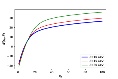
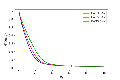
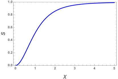
The numerical integration in (37) was carried out using the python package SciPy2020SciPy-NMeth for in the range in GeV and for a wide range in to accommodate a sufficiently large interval around the expected values of the saddle-point in (41). In Fig.1 we plot the resulting functions and for fixed values of GeV in the range alongside the . The function plays the role of the effective instanton-anti-instanton Euclidean action (this is because it arises from integrating the exponent of the classical action over the collective coordinates of non-negative modes of the configuration on the r.h.s. of (37)). The saddle-point value for is given by the equation for each fixed value of , as dictated by (41) above.
Having determined and its derivatives as functions of and we can now carry out the final integration over using the saddle-point approximation formula (42) for the imaginary part of the forward elastic scattering amplitude and hence for the partonic instanton cross-section . Our final results for the partonic instanton cross-section (36) are displayed in Table 1.
Then the hadronic cross-sections are calculated from these partonic cross-sections using the NNPDF3.1luxQED NNLO dataset with Buckley:2014ana Bertone:2017bme and displayed in Table 2. These are calculated using the usual formula
| (44) |
where is the centre-of-mass energy of the hadron collider, is the partonic instanton cross-section and is the minimum invariant mass squared of the produced system. NB here we are only considering the gluon initiated process, otherwise we require a sum over such integrals.
| [GeV] | 50 | 100 | 150 | 200 | 300 | 400 | 500 |
|---|---|---|---|---|---|---|---|
| 9.43 | 11.2 | 12.22 | 12.94 | 13.96 | 14.68 | 15.23 | |
| [pb] | 207.33 | 1.29 | 53.1 | 5.21 | 165.73 | 13.65 | 1.89 |
| [GeV] | 50 | 100 | 150 | 200 | 300 | 400 | 500 |
|---|---|---|---|---|---|---|---|
| 2.62 b | 2.61 nb | 29.6 pb | 1.59 pb | 6.94 fb | 105 ab | 3.06 ab | |
| =1.96 TeV | |||||||
| 58.19 b | 129.70 nb | 2.769 nb | 270.61 pb | 3.04 pb | 114.04 fb | 8.293 fb | |
| =14 TeV | |||||||
| 211.0 b | 400.9 nb | 9.51 nb | 1.02 nb | 13.3 pb | 559.3 fb | 46.3 fb | |
| =30 TeV | |||||||
| 771.0 b | 2.12 b | 48.3 nb | 5.65 nb | 88.3 pb | 4.42 pb | 395.0 fb | |
| =100 TeV |
2.5 Mean number of final state gluons
In our approach of computing the total partonic cross-section via the optical theorem in (36), (37) we have already effectively summed over the number gluons in the final state. This sum can be uncovered by using the series expansion (32) of the exponent of the instanton–anti-instanton action on the right hand side of (37),
| (45) | |||||
The mean value of (i.e. the value that gives the dominant contribution to the integral) is then easily found to be given by the expectation value of the interaction potential,
| (46) |
where the expectation value of is obtained by inserting into the integrand on the right hand side of (36), (37) and normalising by .
In practice, we compute
On the right hand side we have integrated over the variables. The variable is taken to be at its saddle-point value for each fixed value of the energy .
To account for the possibility of the new shifted saddle-point we do this:
3 Instanton Recoil by a Jet
In this section we explain how to generalise the calculation of the instanton process presented above to the case where a jet is emitted from one of the initial state partons. This is of course an important process for collider studies as it allows one to recoil the instanton-generated multi-particle final state by a high- jet.
When the jet is carrying momentum produced from an initial parton , the secondary gluon entering the instanton vertex will necessarily have a virtuality .111In the complimentary scenario where a high- jet is emitted from the instanton vertex in the final state, no virtualities arise, all momenta entering and leaving the instanton vertex are on-shell, and the formalism presented in the earlier section requires no modicfications. In the partonic centre of mass frame we have,
| (49) |
Here we have assumed for simplicity that the jet momentum is transverse, i.e. it does not have a longitudinal component.
The kinematic-invariant CoM energy for the parton-level process is, as before, , where . On the other hand, the invariant mass entering the instanton vertex is now different,
| (50) |
The virtuality of an incoming gluon leg, induced by a no-zero , introduces a multiplicative form-factor into the instanton vertex. This is a well-known result Khoze:1990bm ; Balitsky:1992vs ; Ringwald:1998ek that is a direct consequence of Fourier transforming the instanton field to the momentum space to obtain , where the momentum has a large virtuality, . For the instanton cross-section one needs to compute, , in analogy with Eq. (19), which gives the overall form-factor,
| (51) |
that needs to be included in the integral (LABEL:eq:op_th3). On the right hand side of this equation we used our standard dimensionless variables and defined in (34)-(35).
The second modification of the integral in (LABEL:eq:op_th3), is that the the energy variable corresponds to the instanton vertex energy defined in (50), which is smaller than the overall invariant mass of the parton-level process.
In summary, the instanton parton-level cross-section is computed as follows:
-
1.
For each pair of physical variables , , introduce the auxiliary variables and ,
(52) -
2.
Numerically compute the integral,
(53) and use it to evaluate the expression for the cross-section,
(54) in the saddle-point approximation, as before.
-
3.
The cross-section in physical variables is then obtained via,
(55)
Table 3 presents the results for the instanton cross-section at parton level for a range of partonic CoM energies and for a fixed value of the recoiled jet transverse momentum GeV. The resulting cross-sections fixed are negligibly small. To complement these results we have also computed instanton cross-sections for the case where is scaled with the energy. Table 4 presents the results at parton level where the recoiled jet transverse momentum is chosen as .
| [GeV] | 310 | 350 | 375 | 400 | 450 | 500 |
|---|---|---|---|---|---|---|
| [pb] | 3.42 | 1.35 | 1.06 | 1.13 | 9.23 | 3.10 |
| [GeV] | 100 | 150 | 200 | 300 | 400 | 500 |
|---|---|---|---|---|---|---|
| [pb] | 1.68 | 1.20 | 3.24 | 1.84 | 4.38 | 2.38 |
From the results in Tables 4 and 3 we see that the cross-sections calculated for the processes where the instanton recoils against a jet with large momentum are too small to be observable at any present or envisioned high-energy collider. While increasing the transverse momentum for objects that are difficult to reconstruct by recoiling them against a hard object is often a popular method to improve the sensitivity of the LHC to new physics, see e.g. Kribs:2009yh ; Schlaffer:2014osa ; Harris:2014hga ; Harris:2015kda , the instanton shields itself from such an an option. Consequently, the only way to obtain sensitivity to instantons is to disentangle their spherical radiation profile, made of fairly soft jets, from SM QCD backgrounds.
4 Search for Instanton Events at Hadron Colliders
4.1 Topology of Instanton Events
Since the global event topology of instanton processes is spherically symmetric, and therefore distinctly different from perturbative-QCD events, event shape observables Banfi:2004nk can be a powerful way to identify these processes.
The transverse sphericity tensor is defined as
| (56) |
where run over spatial indices and runs over the number of particles. Here is the two-dimensional transverse component of momentum. The transverse sphericity observable is then defined as where are the eigenvalues of the transverse sphericity tensor and . Transverse sphericity takes values between 0 and 1 with higher values denoting a higher degree of spherical symmetry. Therefore we would expect instanton processes to have a higher transverse sphericity than background processes which in general have some angular dependence.
Spherocity is defined as
| (57) |
where is a unit vector with zero longitudinal component. Again, takes values between 0 and 1, with 1 representing a completely isotropic event and 0 being a pencil-like event. This variable is closely related to thrust which is defined as
| (58) |
where is a unit vector. Thrust is 0 for pencil-like events and 0.5 for spherically symmetric events. The vector which maximises this expression is known as the thrust axis.
The final shape variable we consider is broadening. The thrust axis automatically divides the event into a left hemisphere, and a right hemisphere, . Left and right broadening is then defined as
| (59) |
where is the thrust axis. Total broadening is then the sum of the left and right broadening, , and takes values between 0 and 0.5 with 0.5 being spherically symmetric.
To show the different shapes for these observables between various perturbative SM processes and instanton events at the LHC and the Tevatron, we generate the background events using Pythia 8 Sjostrand:2014zea . For the perturbative SM processes we consider the ones with largest cross-section and jet-rich final states, i.e. high and low-pT multi-jet events, min-bias events, production and +jets events. For the signal we use R AMBO Kleiss:1985gy to populate the phase space of the instanton final state. Each event contains four pairs and a poisson-distributed number of gluons, with a mean in accordance to in Table 1.
All processes are analysed using Fastjet Cacciari:2011ma . For the LHC we reconstruct jets using the anti- algorithm Cacciari:2008gp with a cone-size of and GeV. At the Tevatron jets were analysed using the algorithm Cacciari:2008gp with a cone-size of and were required to have GeV. Leptons are required to have GeV. It should be noted that the instanton processes are not showered or hadronised, but this should not significantly affect the analysis as the position and energy of the reconstructed jets are conserved to a good accuracy.
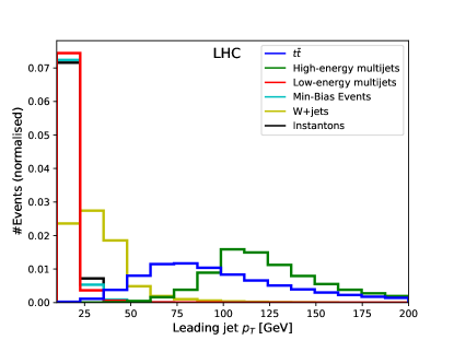
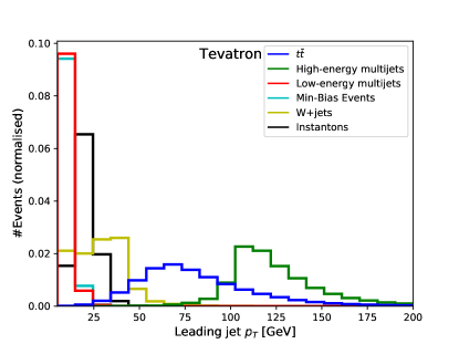
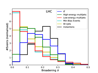
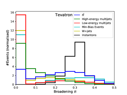
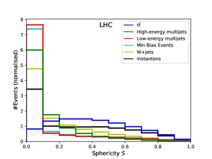
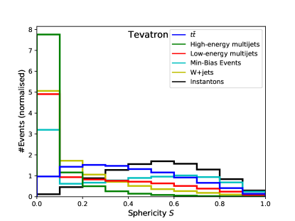
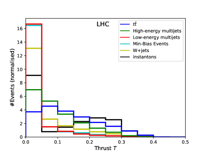
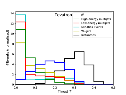
We show in Fig. 2 the distribution for the of the leading jet, in Fig. 3 broadening, in Fig. 4 transverse sphericity and in Fig. 5 thrust for the LHC and the Tevatron respectively. The differences in the histograms between LHC and Tevatron originate in the different jet definitions and thresholds. This leads to more spherical events and thus higher values for thrust and transverse sphericity at the Tevatron. For the backgrounds we include the processes that have the largest perturbatively calculable cross-sections. Most of these processes, in particular high-energy multijets and +jets events, show a more pronounced pencil-like structure than the instanton events. Overall, analysing events with event shape observables provides a powerful method to discriminate instanton events from large Standard Model backgrounds.
4.2 QCD Instanton Search at the LHC
4.2.1 Searches in high-luminosity LHC runs
As a result of the trigger cuts imposed, we find that the LHC has very little sensitivity to QCD instantons in current and future high-luminosity runs. QCD instanton events produce no isolated leptons or a large amount of missing transverse energy, and so appear only as multi-particle events consisting of soft jets.
Missing transverse energy higher-level triggers require at least GeV while single jet triggers are as high as GeV (Aaboud:2016leb, ). In Sec. 3 we have shown that the emission of a hard jet from an initial state parton is not a viable strategy to produce an instanton. Further, the probability that one of the partons that originates in the instanton process has such a large momentum is very small as well. If one of the instanton-induced partons has a transverse momentum to pass the single-jet trigger requirements, the centre-of-mass energy of the instanton has to be at least of GeV. According to Table 2, this renders the hadronic instanton cross-section too small to be observable.
Thus, one would have to resort to multijet triggers, either with four jets of GeV or six jets of GeV. Both such trigger requirements result in for instantons fairly high partonic centre-of-mass energies of GeV. Generating 100000 signal events as described in Sec. 4.1 and reconstructing them with the anti-kT jet algorithm, we find that none of the events passes multijet triggers, which results in an upper limit on the instanton cross-section that passes such trigger cuts of fb. Disentangling instanton processes with less than fb of cross-section from large QCD backgrounds during the event reconstruction step is a highly challenging task.
Due to increased pileup in future high-luminosity LHC runs and at future hadron colliders, e.g. the FCC-hh, trigger thresholds for jets will have to be increased, which will significantly reduce sensitivity to QCD instanton processes. Special trigger strategies would have to be developed for instantons to pass trigger requirements in such a jet-rich environment. One could speculate about the inclusion of event-shape observables directly in the trigger strategy and a highly optimised interplay between high-level and low-level triggers. As shown in Sec. 4.1 in Figs. 2, 3, 4 and 5 instanton events have a very different event topology compared to QCD-induced multi-jet or resonance-associated production processes. Incorporating such observables in the trigger setup and reconstruction strategies might retain some sensitivity to instanton processes in future runs at high-energy hadron colliders.
4.2.2 Search in low-luminosity LHC runs
Rather than focusing on high-luminosity runs, we propose to pursue a different search strategy. The biggest obstacles to the discovery of QCD instanton processes are the high trigger thresholds, which are a necessity to avoid triggering on pileup in high-luminosity runs. Low-luminosity LHC runs had minimalistic trigger requirements (ATLAS:2020cap, ), i.e. min-bias triggers which required only a single charged track with an energy of 400 MeV. Remarkably, practically all QCD instanton events would pass min-bias triggers. ATLAS and CMS CMS:2018elu both are in possession of un-prescaled min-bias datasets which are however often only used to determine the luminosity for low-pileup runs, rather than searching for new phenomena.
To assess whether these datasets can provide sensitivity to QCD instanton processes, we generate event samples as outlined in Sec. 4.1 with a hadronic centre-of-mass energy of TeV. For the event selection we require that each event should have at least six jets with a minimum GeV and that these jets form a thrust value of . This already confidently separates instanton signal events from QCD-induced background events. For an instanton with a minimum GeV, which can be imposed through a requirement on the invariant mass of the final state jets, we find and for GeV we have . This shows a very good sensitivity for instanton processes in min-bias events, which can be further increased by lowering the requirements.
4.3 QCD Instanton Search at the Tevatron
We deduce from the observations in Sec. 4.2.1 that future runs at high-energy high-luminosity colliders are likely to become even less sensitive to QCD instanton processes. Consequently, looking into the other direction instead, e.g. at the Tevatron, might provide yet another way to search for QCD instantons. In the top row of Table 2 we show the hadronic cross-sections at Tevatron energies, depending on the partonic centre-of-mass energy of the instanton process.
We recast several jet-rich searches and measurements by CDF (Aaltonen:2011vi, ; Aaltonen:2011kx, ; Collaboration:2012hz, ). While a large fraction of instanton events would pass the trigger criteria, the event selection criteria applied in the analysis removed the predominant fraction of instanton events. Thus, the results provided in (Aaltonen:2011vi, ; Aaltonen:2011kx, ; Collaboration:2012hz, ) did not allow to set an experimental constraint on the instanton cross-section. However, if this data was reanalysed and event reconstruction strategies following Secs. 4.1 and 4.2.1 were applied, the Tevatron could set stringent limits on the hadronic instanton cross-section.
5 Conclusions
Instantons are the best motivated, yet unobserved, non-perturbative effects predicted by the Standard Model. Being able to study instantons in scattering processes would provide a new window to the phenomenological exploration of the QCD vacuum and it would allow the tensioning of non-perturbative theoretical methods developed for gauge theories with data.
In our calculation we used the optical theorem to calculate the total instanton cross-section from the elastic scattering amplitude by carrying out an integral over the instanton collective coordinates, and taking into account the hard-hard initial state interactions calculated in (Mueller:1990qa, ). The inclusion of these interactions is essential as it provides a cut-off for the integral over the instanton scale size which otherwise diverges in the IR in any QCD-like theory when no explicit external scales (such as the scalar field VEVs, highly virtual momenta or high temperature) are present. This theoretical approach was first presented and applied recently in Khoze:2019jta . We improved on the results of Khoze:2019jta here by using a more robust integration method by directly computing integrals over all instanton–anti-instanton collective coordinates that correspond to positive modes of the quadratic fluctuation operators in the instanton–anti-instanton background. This resulted in an increase to the instanton cross-section by approximately an order of magnitude, compared to the saddle-point approximation used previously. We then also calculated the mean number of gluons in the final state using a novel and more direct approach based on computing the expectation value of the instanton–anti-instanton interaction potential.
Most of the earlier studies of QCD instanton-induced processes, prior to Ref. Khoze:2019jta , were specific to deep-inelastic scattering (DIS) Balitsky:1992vs ; Ringwald:1998ek ; Ringwald:2003px . In this case, it was the deep inelastic momentum scale that was essential for obtaining infrared safe instanton contributions in the DIS settings and at relatively low CoM energies. The H 1 and Z EUS Collaborations have searched for QCD instantons at the H ERA collider Adloff:2002ph ; Chekanov:2003ww ; H1:2016jnv . In the electroweak sector of the Standard Model, phenomenological consequences of similar non-perturbative processes were also studied in detail in the literature, including recent papers Ringwald:2018gpv ; Papaefstathiou:2019djz ; Ellis:2016dgb , and references therein. In particular, Ref. Khoze:2020paj relied on applying the theoretical formalism developed here and in Khoze:2019jta , with the conclusion that electroweak instanton contributions at colliders are exponentially suppressed at all energies.
In this paper we have re-examined the phenomenology of QCD instanton contributions to high-energy scattering processes at hadron colliders. We showed that although the instanton cross-sections are very large in a hadron collider; surprisingly such colliders have little sensitivity to instantons due to the trigger criteria necessary to reduce the data rate. Although instantons produce many final state particles, the event is isotropic and the energy is divided between all particles resulting in few particles with large , one of the principle trigger requirements in a hadron collider. The higher energy instantons which could potentially pass such triggers have a vanishingly small cross-section and would not be seen in sufficient numbers in the LHC to be distinguishable from the QCD background. However examination of data collected with a minimum bias trigger (ATLAS:2020cap, ; CMS:2018elu, ) showed that it should be possible to either discover instantons or severely constrain their cross-section with such data, which was previously only used for luminosity calibration. We also examined data from the Tevatron and showed that certain triggers should have recorded many instanton events on tape but the selection criteria used in later analyses would render the analyses insensitive to instantons. With a new set of selection criteria this would also be another possible avenue for discovery.
Acknowledgements
We thank Deepak Kar, Frank Krauss and Matthias Schott for helpful discussions. We acknowledge funding from the STFC under grant ST/P001246/1.
Appendix: A. Instanton–anti-instanton valley configuration
The forward elastic scattering amplitude is obtained from the LSZ-reduced Green’s function is calculated using the the path integral in the instanton–anti-instanton background,
| (A.60) |
The definition and the meaning of the instanton–anti-instanton field configuration is provided by the valley method approach of Balitsky and Yung, (Balitsky:1986qn, ; Yung:1987zp, ) and the computation of the instanton cross-section using the optical theorem approach follows the approach developed in Khoze:1990bm ; Khoze:1991mx ; Khoze:1991sa ; Verbaarschot:1991sq and applied to QCD instantons at proton colliders in the recent paper Khoze:2019jta .
Usually when performing a functional integral such as this, we would expand the action around the minimum, recalling that the linear term vanishes as instantons satisfy the equations of motion, and we would get the functional determinant of but here we must be careful. If this operator possesses small or zero eigenvalues then the usual will become very large or singular as the Gaussian approximation fails. We must treat these zero/quasizero modes carefully. These modes arise when there is a symmetry or approximate symmetry of the system leaving the action unchanged.
A typical example of a zero mode is the centre of the BPST instanton, the corresponding collective coordinate does not affect the value of the instanton action and so translation is a symmetry. In general each symmetry of the system that is broken by the background field configuration (in our case the instanton) will have an associated collective coordinate, , with zero mode , where denotes the background field.
Quasi-zero modes can be understood in a similar fashion even though they do not correspond to an exact symmetry of the system. A typical example of a quasi-zero mode is the separation between the positions of the instanton and the anti-instanton in the instanton–anti-instanton configuration. At large separations, the individual (anti)-instantons interact very weakly and the collective coordinate that corresponds to their separation becomes a nearly flat direction of the instanton–anti-instanton action. Once again we denote the background instanton–anti-instanton field configuration and the quasi-zero mode is given by . In general will now denote the set of all collective coordinates, for the zero and quasi-zero modes.
The background field configuration with a quasi-zero mode (i.e. a nearly flat direction in the action parameterised by the coordinate) can now be defined as a solution of the gradient flow equation, also known as the valley equation of Balitsky and Yung (Balitsky:1986qn, ; Yung:1987zp, ),
| (A.61) |
If the background field is an exact classical solution, then the -collective-coordinate parameterises an exact zero mode and we have so the valley equation collapses to the Euler-Lagrange equation. However, in the case of a quasi-zero mode, is a pseudo-flat direction; the action is not at the exact minimum at any fixed value of . In this case the equation (A.64) holds with a non-vanishing but small right hand side, so that . The smallness of the parameter characterises how flat the corresponding quasi-zero mode is.
To proceed with our calculation of the Green’s function one uses the Fadeev-Popov procedure (Balitsky:1986qn, ; Yung:1987zp, ):
| (A.62) |
where is the minimum of the action for fixed and denotes the scalar product or an overlap of two field configurations,
| (A.63) |
Note that the definition of the overlap above uses a positive weight function – the freedom to choose a convenient form of is a well-known simplifying feature used in path integral expansions around instantons tHooft:1976snw ; Levine:1978ge ; Yung:1987zp and will be utilised in what follows. Taking into account the weight factor, the valley equation reads,
| (A.64) |
Inserting one of the factors of 1 in the form (A.62) for each collective coordinate, and expanding the action around the background field ,
we get,
| (A.66) |
where . We note that the term linear in fluctuations in the expansion of the action (the second term on the right hand side of (Acknowledgements)) in fact does not contribute to the integral in (A.66). Indeed, the valley equation (A.64) requires that is proportional to when computed on our background configuration and then the delta-function in the integrand (A.66) ensures that this linear term vanishes.
Now we can perform the functional integration (Yung:1987zp, ),
| (A.67) |
Since the play the role of zero- and quasi-zero modes of the action, they are the eigenfunctions of and so,
| (A.68) |
This equation is valid at the leading order in the small parameter and follows from differentiating both sides of the valley equation with respect to and neglecting the term.
This allows us to simplify the product of the three determinants in (A.67) into
| (A.69) |
where denotes the determinant with the zero and quasi-zero modes removed ( modes for the instantons and modes for the anti-instanton).
To the leading order in the small- expansion we can also factorise the quadratic fluctuation determinant in the instanton–anti-instanton background into the product of the instanton and the anti–instanton quadratic fluctuation determinants, .
This gives us finally (Yung:1987zp, ),
| (A.70) |
where
| (A.71) |
are the instanton and anti-instanton collective coordinate integration measurse.
Having established the form of the collective coordinate integrals for the instanton-anti-instanton case, what is left for us to determine is the instanton–anti-instanton configuration itself and in particular its action as the function of (anti)-instanton collective coordinates.
The instanton–anti-instanton valley trajectory was obtained in Ref. (Yung:1987zp, ) by finding an exact solution of the valley equation (A.64) for a particular choice of the weight function by exploring conformal invariance of the classical Yang-Mills action. The action on this configuration was computed in Khoze:1991sa and Khoze:1991mx ; Verbaarschot:1991sq and it takes the form,
| (A.72) |
where the variable is the conformal ratio of the (anti)-instanton collective coordinates,
| (A.73) |
plays the role of the single negative quasi-zero mode of the instanton–anti-instanton valley configuration.
In the limit of large separation between the instanton centres, , the conformal ratio , and instanton–anti-instanton action becomes the sum of the indiidual instanton and anti-instanton actions,
| (A.74) |
and
| (A.75) |
In the opposite limit of a vanishing separation between the instanton centres, , the conformal ratio and the expression for the action goes to zero. This is in agreement with the expectation that in this limit the instanton and the anti-instanton annihilate to the perturbative vacuum .
We can plot the action as the function of the separation between the instanton centres normalised by the instanton scale sizes. For simplicity, if we assume that the sizes are equal, we can write down the action as the function of the vartiable . It is plotted in Fig. 6 in units of .
Appendix: B. Integration over the relative orientations
To be able to integrate over relative orientations in the internal space, we need to know the form of the instanton–anti-instanton action for arbitrary values of their relative orientation matrix . However our exact valley configuration is only known for the maximally attractive channel, i.e. where the interaction potential is maximised over the relative orientations for at each fixed value of .
What is known, however is the form of the interaction potential in the limit of large separations. In this large-separations regime (i.e. ) the instanton and the anti-instanton are known to have dipole-dipole interactions Callan:1977gz ,
| (B.76) |
where is the matrix in the upper-left corner of the matrix describing the relative instanton–anti-instanton orientation.222The upper-left corner is selected by placing the instanton in the upper-left corner while allowing the anti-instanton to be anywhere in the of the internal space.
Lacking the precise solution of the instanton–anti-instanton valley for general orientations at arbitrary separations, we will simply assume that the full interaction potential can always be written in the form (c.f. (30)),
| (B.77) |
where is the maximally-attractive-orienatation potential (28),(21). Clearly at large separations, to order this expression coincides with the known dipole-dipole interaction.
We can now represent the integral over the relative orientations as follows,
| (B.78) |
These type of integrals over matrices have been previously computed in the instanton literature, see Eq. (2.15) in Balitsky:1992vs :
| (B.79) |
Substituting to the expression above, we now obtain the answer for our relative orientation integral in (B.78),
| (B.80) |
which agrees with the expression (33) quoted in section 2.
References
- (1) V. V. Khoze, F. Krauss, and M. Schott, “Large Effects from Small QCD Instantons: Making Soft Bombs at Hadron Colliders,” JHEP 04 (2020) 201, [arXiv:1911.09726 [hep-ph]].
- (2) C. G. Callan, Jr., R. F. Dashen, and D. J. Gross, “The Structure of the Gauge Theory Vacuum,” Phys. Lett. 63B (1976) 334–340.
- (3) R. Jackiw and C. Rebbi, “Vacuum Periodicity in a Yang-Mills Quantum Theory,” Phys. Rev. Lett. 37 (1976) 172–175.
- (4) A. A. Belavin, A. M. Polyakov, A. S. Schwartz, and Yu. S. Tyupkin, “Pseudoparticle Solutions of the Yang-Mills Equations,” Phys. Lett. B59 (1975) 85–87.
- (5) G. ’t Hooft, “Computation of the Quantum Effects Due to a Four-Dimensional Pseudoparticle,” Phys. Rev. D14 (1976) 3432–3450. [Erratum: Phys. Rev.D18,2199(1978)].
- (6) G. ’t Hooft, “Symmetry Breaking Through Bell-Jackiw Anomalies,” Phys. Rev. Lett. 37 (1976) 8–11.
- (7) V. V. Khoze and A. Ringwald, “Nonperturbative contribution to total cross-sections in non-Abelian gauge theories,” Phys. Lett. B259 (1991) 106–112.
- (8) A. V. Yung, “Instanton Vacuum in Supersymmetric QCD,” Nucl. Phys. B297 (1988) 47.
- (9) A. H. Mueller, “Leading power corrections to the semiclassical approximation for gauge meson collisions in the one instanton sector,” Nucl. Phys. B353 (1991) 44–58.
- (10) A. H. Mueller, “First Quantum Corrections to Gluon-gluon Collisions in the One Instanton Sector,” Nucl. Phys. B348 (1991) 310–326.
- (11) S. Knapen, S. Pagan Griso, M. Papucci, and D. J. Robinson, “Triggering Soft Bombs at the LHC,” JHEP 08 (2017) 076, [arXiv:1612.00850 [hep-ph]].
- (12) S. Coleman, Aspects of Symmetry: Uses of Instantons. Cambridge University Press, Cambridge, U.K., 1985.
- (13) A. I. Vainshtein, V. I. Zakharov, V. A. Novikov, and M. A. Shifman, “ABC’s of Instantons,” Sov. Phys. Usp. 25 (1982) 195. [Usp. Fiz. Nauk136,553(1982)].
- (14) M. P. Mattis, “The Riddle of high-energy baryon number violation,” Phys. Rept. 214 (1992) 159–221.
- (15) T. Schafer and E. V. Shuryak, “Instantons in QCD,” Rev. Mod. Phys. 70 (1998) 323–426, [arXiv:hep-ph/9610451 [hep-ph]].
- (16) N. Dorey, T. J. Hollowood, V. V. Khoze, and M. P. Mattis, “The Calculus of many instantons,” Phys. Rept. 371 (2002) 231–459, [arXiv:hep-th/0206063 [hep-th]].
- (17) G. ’t Hooft, “How Instantons Solve the U(1) Problem,” Phys. Rept. 142 (1986) 357–387.
- (18) A. Hasenfratz and P. Hasenfratz, “The Scales of Euclidean and Hamiltonian Lattice QCD,” Nucl. Phys. B193 (1981) 210.
- (19) M. Luscher, “A Semiclassical Formula for the Topological Susceptibility in a Finite Space-time Volume,” Nucl. Phys. B205 (1982) 483–503.
- (20) A. Ringwald, “High-Energy Breakdown of Perturbation Theory in the Electroweak Instanton Sector,” Nucl. Phys. B330 (1990) 1–18.
- (21) P. B. Arnold and L. D. McLerran, “Sphalerons, Small Fluctuations and Baryon Number Violation in Electroweak Theory,” Phys. Rev. D36 (1987) 581.
- (22) I. I. Balitsky and A. V. Yung, “Collective - Coordinate Method for Quasizero Modes,” Phys. Lett. 168B (1986) 113–119. [,273(1986)].
- (23) V. V. Khoze and A. Ringwald, “Valley trajectories in gauge theories,” CERN-TH-6082-91 (1991) . https://lib-extopc.kek.jp/preprints/PDF/1991/9106/9106100.pdf.
- (24) J. Verbaarschot, “Streamlines and conformal invariance in Yang-Mills theories,” Nucl. Phys. B 362 (1991) 33–53. [Erratum: Nucl.Phys.B 386, 236–236 (1992)].
- (25) I. I. Balitsky and V. M. Braun, “Instanton-induced contributions of fractional twist in the cross-section of hard gluon-gluon scattering in QCD,” Phys. Rev. D47 (1993) 1879–1888.
- (26) E. V. Shuryak and J. Verbaarschot, “On baryon number violation and nonperturbative weak processes at SSC energies,” Phys. Rev. Lett. 68 (1992) 2576–2579.
- (27) A. Ringwald and F. Schrempp, “Instanton induced cross-sections in deep inelastic scattering,” Phys. Lett. B438 (1998) 217–228, [arXiv:hep-ph/9806528 [hep-ph]].
- (28) P. Virtanen, R. Gommers, T. E. Oliphant, M. Haberland, T. Reddy, D. Cournapeau, and et al., “SciPy 1.0: Fundamental Algorithms for Scientific Computing in Python,” Nature Methods 17 (2020) 261–272.
- (29) A. Buckley, J. Ferrando, S. Lloyd, K. Nordstrom, B. Page, M. Refenacht, M. Schonherr, and G. Watt, “LHAPDF6: parton density access in the LHC precision era,” Eur. Phys. J. C 75 (2015) 132, [arXiv:1412.7420 [hep-ph]].
- (30) NNPDF Collaboration, V. Bertone, S. Carrazza, N. P. Hartland, and J. Rojo, “Illuminating the photon content of the proton within a global PDF analysis,” SciPost Phys. 5 no. 1, (2018) 008, [arXiv:1712.07053 [hep-ph]].
- (31) V. V. Khoze and A. Ringwald, “Total cross-section for anomalous fermion number violation via dispersion relation,” Nucl. Phys. B355 (1991) 351–368.
- (32) G. D. Kribs, A. Martin, T. S. Roy, and M. Spannowsky, “Discovering the Higgs Boson in New Physics Events using Jet Substructure,” Phys. Rev. D 81 (2010) 111501, [arXiv:0912.4731 [hep-ph]].
- (33) M. Schlaffer, M. Spannowsky, M. Takeuchi, A. Weiler, and C. Wymant, “Boosted Higgs Shapes,” Eur. Phys. J. C 74 no. 10, (2014) 3120, [arXiv:1405.4295 [hep-ph]].
- (34) P. Harris, V. V. Khoze, M. Spannowsky, and C. Williams, “Constraining Dark Sectors at Colliders: Beyond the Effective Theory Approach,” Phys. Rev. D 91 (2015) 055009, [arXiv:1411.0535 [hep-ph]].
- (35) P. Harris, V. V. Khoze, M. Spannowsky, and C. Williams, “Closing up on Dark Sectors at Colliders: from 14 to 100 TeV,” Phys. Rev. D 93 no. 5, (2016) 054030, [arXiv:1509.02904 [hep-ph]].
- (36) A. Banfi, G. P. Salam, and G. Zanderighi, “Resummed event shapes at hadron - hadron colliders,” JHEP 08 (2004) 062, [arXiv:hep-ph/0407287].
- (37) T. Sjöstrand, S. Ask, J. R. Christiansen, R. Corke, N. Desai, P. Ilten, S. Mrenna, S. Prestel, C. O. Rasmussen, and P. Z. Skands, “An introduction to PYTHIA 8.2” Comput. Phys. Commun. 191 (2015) 159–177, [arXiv:1410.3012 [hep-ph]].
- (38) R. Kleiss, W. J. Stirling, and S. D. Ellis, “A New Monte Carlo Treatment of Multiparticle Phase Space at High-energies,” Comput. Phys. Commun. 40 (1986) 359.
- (39) M. Cacciari, G. P. Salam, and G. Soyez, “FastJet User Manual,” Eur. Phys. J. C 72 (2012) 1896, [arXiv:1111.6097 [hep-ph]].
- (40) M. Cacciari, G. P. Salam, and G. Soyez, “The anti- jet clustering algorithm,” JHEP 04 (2008) 063, [arXiv:0802.1189 [hep-ph]].
- (41) ATLAS Collaboration, M. Aaboud et al., “Performance of the ATLAS Trigger System in 2015,” Eur. Phys. J. C 77 no. 5, (2017) 317, [arXiv:1611.09661 [hep-ex]].
- (42) ATLAS Collaboration, “Luminosity determination for low-pileup datasets at and 13 TeV using the ATLAS detector at the LHC,”.
- (43) CMS Collaboration, “CMS luminosity measurement for the 2017 data-taking period at ,”.
- (44) CDF Collaboration, T. Aaltonen et al., “Search for resonant production of decaying to jets in collisions at TeV,” Phys. Rev. D 84 (2011) 072003, [arXiv:1108.4755 [hep-ex]].
- (45) CDF Collaboration, T. Aaltonen et al., “Top-quark mass measurement using events with missing transverse energy and jets at CDF,” Phys. Rev. Lett. 107 (2011) 232002, [arXiv:1109.1490 [hep-ex]].
- (46) CDF Collaboration, T. Aaltonen et al., “Measurements of the Top-quark Mass and the Cross Section in the Hadronic Jets Decay Channel at TeV,” Phys. Rev. Lett. 109 (2012) 192001, [arXiv:1208.5720 [hep-ex]].
- (47) A. Ringwald, “From QCD instantons at HERA to electroweak B + L violation at VLHC,” [arXiv:hep-ph/0302112 [hep-ph]]. [PoSjhw2002,008(2002)].
- (48) H1 Collaboration, C. Adloff et al., “Search for QCD instanton induced processes in deep inelastic scattering at HERA,” Eur. Phys. J. C25 (2002) 495–509, [arXiv:hep-ex/0205078 [hep-ex]].
- (49) ZEUS Collaboration, S. Chekanov et al., “Search for QCD instanton induced events in deep inelastic ep scattering at HERA,” Eur. Phys. J. C34 (2004) 255–265, [arXiv:hep-ex/0312048 [hep-ex]].
- (50) H1 Collaboration, V. Andreev et al., “Search for QCD instanton-induced processes at HERA in the high- domain,” Eur. Phys. J. C76 no. 7, (2016) 381, [arXiv:1603.05567 [hep-ex]].
- (51) A. Ringwald, K. Sakurai, and B. R. Webber, “Limits on Electroweak Instanton-Induced Processes with Multiple Boson Production,” JHEP 11 (2018) 105, [arXiv:1809.10833 [hep-ph]].
- (52) A. Papaefstathiou, S. Platzer, and K. Sakurai, “On the phenomenology of sphaleron-induced processes at the LHC and beyond,” [arXiv:1910.04761 [hep-ph]].
- (53) J. Ellis, K. Sakurai, and M. Spannowsky, “Search for Sphalerons: IceCube vs. LHC,” JHEP 05 (2016) 085, [arXiv:1603.06573 [hep-ph]].
- (54) V. V. Khoze and D. L. Milne, “Suppression of Electroweak Instanton Processes in High-energy Collisions,” [arXiv:2011.07167 [hep-ph]].
- (55) H. Levine and L. G. Yaffe, “Higher Order Instanton Effects,” Phys. Rev. D 19 (1979) 1225.
- (56) C. G. Callan, Jr., R. F. Dashen, and D. J. Gross, “Toward a Theory of the Strong Interactions,” Phys. Rev. D17 (1978) 2717.