Wind-induced changes to surface gravity wave shape in shallow water

Abstract

Wave shape (e.g. wave skewness and asymmetry) impacts sediment transport, remote sensing and ship safety. Previous work showed that wind affects wave shape in intermediate and deep water. Here, we investigate the effect of wind on wave shape in shallow water through a wind-induced surface pressure for different wind speeds and directions to provide the first theoretical description of wind-induced shape changes. A multiple-scale analysis of long waves propagating over a shallow, flat bottom and forced by a Jeffreys-type surface pressure yields a forward or backward Korteweg–de Vries (KdV)–Burgers equation for the wave profile, depending on the wind direction. The evolution of a symmetric, solitary-wave initial condition is calculated numerically. The resulting wave grows (decays) for onshore (offshore) wind and becomes asymmetric, with the rear face showing the largest shape changes. The wave profile’s deviation from a reference solitary wave is primarily a bound wave and trailing, dispersive, decaying tail. The onshore wind increases the wave’s energy and skewness with time while decreasing the wave’s asymmetry, with the opposite holding for offshore wind. The corresponding wind speeds are shown to be physically realistic, and the shape changes are explained as slow growth followed by rapid evolution according to the unforced KdV equation.

1 Introduction

The study of wind and ocean wave interactions began with Jeffreys (1925) and continues to be an active field of research (e.g. Janssen, 1991; Donelan et al., 2006; Sullivan & McWilliams, 2010). Many theoretical studies (e.g. Jeffreys, 1925; Miles, 1957; Phillips, 1957) focus on calculating wind-induced growth rates and often employ phase-averaging techniques. However, experimental (e.g. Leykin et al., 1995; Feddersen & Veron, 2005) and theoretical (e.g. Zdyrski & Feddersen, 2020) studies have shown wind can also influence wave shape, quantified by third-order shape statistics such as skewness and asymmetry, corresponding to vertical and horizontal asymmetry, respectively. Furthermore, while many numerical studies on coupled wind and waves employ sinusoidal water waves and therefore neglect wind-induced shape changes (e.g. Hara & Sullivan, 2015; Husain et al., 2019), some recent numerical studies have incorporated wind-induced changes to the wave field using coupled air–water simulations (e.g. Liu et al., 2010; Hao & Shen, 2019) or direct numerical simulations of two-fluid flows (e.g. Zonta, Soldati & Onorato, 2015; Yang, Deng & Shen, 2018). Wave shape influences sediment transport, affecting beach morphodynamics (e.g. Drake & Calantoni, 2001; Hoefel & Elgar, 2003), while wave skewness affects radar altimetry signals (e.g. Hayne, 1980) and asymmetry influences ship responses to wave impacts (e.g. Soares, Fonseca & Pascoal, 2008).

Waves in shallow water, where $kh\ll 1$ (with $h$ the water depth, $k=2\pi/\lambda$ the wavenumber and $\lambda$ the wavelength), differ qualitatively from those in intermediate ($kh\sim 1$) to deep ($kh\gg 1$) water. For waves with small amplitudes $a_{0}\ll h$, leveraging the small parameters $a_{0}/h\sim(kh)^{2}\ll 1$ yields the Boussinesq equations with weak dispersion and nonlinearity. When dispersion balances nonlinear focusing, a special class of waves, known as solitary waves, are formed and appear in environments ranging from nonlinear optical pulses (e.g. Kivshar, 1993) to astrophysical dusty plasmas (e.g. Sahu & Tribeche, 2012). These well-understood waves are often used to study fluid dynamical (e.g. Munk, 1949; Hammack & Segur, 1974; Miles, 1979; Lin & Liu, 1998) and engineering (e.g. Monaghan & Kos, 1999; Lin, 2004; Xu, Chen & Chen, 2018) contexts owing to their simplicity. One of the simplest equations displaying solitary waves is the Korteweg–de Vries (KdV) equation, which incorporates dispersion and nonlinearity. When augmented with a dissipative term, this becomes the KdV–Burgers equation, with applications to damped internal tides (e.g. Sandstrom & Oakey, 1995), electron waves in graphene (e.g. Zdyrski & McGreevy, 2019) and viscous flow in blood vessels (e.g. Antar & Demiray, 1999). While field observations (e.g. Cavaleri & Rizzoli, 1981) have investigated the wind-induced growth of shallow-water waves, the interaction of wind and shallow-water waves has not yet been formulated into a simple equation such as the KdV–Burgers equation.

The influence of wind on wave shape has been previously investigated in intermediate and deep water (Zdyrski & Feddersen, 2020). However, the coupling between wind and wave shape has not yet been investigated in shallow water. To investigate wind and surface wave interactions in shallow water over a flat bottom, we introduce a wind-induced pressure term to the Boussinesq equations in § 2. The resulting KdV–Burgers equation governs a solitary wave’s evolution, which we solve numerically to yield the wave’s energy, skewness and asymmetry in § 3. We calculate the wind speed, discuss the asymmetry and compare our results to intermediate- and deep-water waves in § 4.

2 Derivation of the KdV–Burgers equation

2.1 Governing equations

We treat the flow as irrotational and inviscid and neglect surface tension. Furthermore, we restrict ourselves to planar wave propagation in the $+x$ direction. Finally, we choose a coordinate system with $z=0$ at the mean water level and a horizontal, flat bottom located at $z=-h$. Then, the incompressibility condition and standard boundary conditions are

$$0 =\phi_{xx}+\phi_{zz} \mbox{\quad on\quad}-h<z<\eta,$$ (1)

$$0 =\phi_{z} \mbox{\quad on\quad}z=-h,$$ (2)

$$\phi_{z} =\eta_{t}+\phi_{x}\eta_{x} \mbox{\quad on\quad}z=\eta,$$ (3)

$$0 =\frac{p}{\rho_{w}}+g\eta+\phi_{t}+\frac{1}{2}\bqty{\phi_{x}^{2}+\phi_{z}^{2}} \mbox{\quad on\quad}z=\eta.$$ (4)

Here, $\eta(x,t)$ is the wave profile, $\phi(x,z,t)$ is the flow’s velocity potential related to the velocity $\mathbf{\bm{u}}=\gradient{\phi}$, $p(x,t)$ is the surface pressure, $g$ is the gravitational acceleration and $\rho_{w}$ is the water density. We used the $\phi$ gauge freedom to absorb the Bernoulli ‘constant’ $C(t)$ in the dynamic boundary condition. We seek a solitary, progressive wave which decays at infinity, $\eta(\mathbf{\bm{x}},t)\to 0$ as $\absolutevalue{\mathbf{\bm{x}}}\to\infty$, with similar conditions on $\mathbf{\bm{u}}$. We choose a coordinate system where the average bottom horizontal velocity vanishes,

$$\overline{\partialderivative{\phi}{x}}=0\mbox{\quad on\quad}z=-h,$$ (5)

with the overline a spatial average $\overline{f}\coloneqq\lim_{L\to\infty}\int_{-L}^{L}f\differential{x}/(2L)$. Additionally, we assume the surface pressure $p(x,t)$ is a Jeffreys-type forcing (Jeffreys, 1925),

$$p(x,t)=P\partialderivative{\eta(x,t)}{x}.$$ (6)

Here, $P$ is proportional to $(U-c)^{2}$, with $c$ the wave’s nonlinear phase speed and $U$ the wind speed (cf. § 4.1). Note that $P>0$ corresponds to (‘onshore’) wind in the same direction as the wave while $P<0$ denotes (‘offshore’) wind opposite the wave. We use a Jeffreys forcing for its analytic simplicity and clear demonstration of wind–wave coupling. Jeffrey’s separated sheltering mechanism is likely only relevant in special situations (e.g. near breaking, Banner & Melville, 1976, or for steep waves under strong winds, Touboul & Kharif, 2006; Tian & Choi, 2013). Additionally, numerical simulations of sinusoidal waves suggest the peak surface pressure is shifted approximately $135\text{\,}\mathrm{\SIUnitSymbolDegree}$ from the wave peak, while Jeffreys would give a $90\text{\,}\mathrm{\SIUnitSymbolDegree}$ shift (Husain et al., 2019). However, a fully dynamic coupling between wind and waves — necessary for an accurate surface pressure over a non-sinusoidal, dynamic water surface — is outside the scope of this paper. Furthermore, the applicability of Jeffreys forcing to extreme waves means our theory could apply to the wind forcing of rogue waves in shallow water (Kharif et al., 2008).

2.2 Non-dimensionalization

We non-dimensionalize our system with the known characteristic scales: the horizontal length scale $L$ over which $\eta$ changes rapidly, expressed as an effective wavenumber $k_{E}\coloneqq 2\pi/L$; the (initial) wave amplitude $a_{0}=H_{0}/2$ (i.e. half the wave height $H_{0}$); the depth $h$; the gravitational acceleration $g$; and the wind speed $U$, expressed as a pressure magnitude $P\propto\rho_{a}(U-c)^{2}$, with $\rho_{a}\approx$1.225\text{\times}{10}^{-3}$\rho_{w}$ the density of air. Denoting non-dimensional variables with primes, we have

$$\begin{aligned} x&=\frac{x^{\prime}}{k_{E}}=h\frac{x^{\prime}}{\sqrt{\mu_{E}}},\\ z&=hz^{\prime},\end{aligned}\qquad\begin{aligned} t&=\frac{t^{\prime}}{k_{E}c_{0}}=\frac{t^{\prime}}{\sqrt{\mu_{E}}}\sqrt{\frac{h}{g}},\\ P&=\varepsilon P^{\prime}\frac{\rho_{w}g}{k_{E}}=\frac{\varepsilon}{\sqrt{\mu_{E}}}P^{\prime}\rho_{w}c_{0}^{2},\end{aligned}\qquad\begin{aligned} \eta&=a_{0}\eta^{\prime}=h\varepsilon\eta^{\prime},\\ \phi&=\phi^{\prime}\frac{a_{0}}{k_{E}}\sqrt{\frac{g}{h}}=\frac{\phi^{\prime}\varepsilon}{\sqrt{\mu_{E}}}c_{0}h,\end{aligned}$$ (7)

with linear, shallow-water phase speed $c_{0}=\sqrt{gh}$. Our system’s dynamics is controlled by three small, non-dimensional parameters: $\varepsilon\coloneqq a_{0}/h$, $\mu_{E}\coloneqq(k_{E}h)^{2}$ and $Pk_{E}/(\rho_{w}g)$. We will later require $\order{\varepsilon}=\order{\mu_{E}}=\order{Pk_{E}/(\rho_{w}g)}$. Now, our non-dimensional equations take the form

$$0 =\mu_{E}\phi^{\prime}_{x^{\prime}x^{\prime}}+\phi^{\prime}_{z^{\prime}z^{\prime}} \mbox{\quad on\quad}-1<z^{\prime}<\varepsilon\eta^{\prime},$$ (8)

$$0 =\phi^{\prime}_{z^{\prime}} \mbox{\quad on\quad}z^{\prime}=-1,$$ (9)

$$\phi^{\prime}_{z^{\prime}} =\mu_{E}\eta^{\prime}_{t^{\prime}}+\varepsilon\mu_{E}\phi^{\prime}_{x^{\prime}}\eta^{\prime}_{x^{\prime}} \mbox{\quad on\quad}z^{\prime}=\varepsilon\eta^{\prime},$$ (10)

$$0 =\varepsilon P^{\prime}\eta^{\prime}_{x^{\prime}}+\eta^{\prime}+\phi^{\prime}_{t^{\prime}}+\frac{1}{2}\pqty{\varepsilon\phi_{x^{\prime}}^{\prime.2}+\frac{\varepsilon}{\mu_{E}}\phi_{z^{\prime}}^{\prime.2}} \mbox{\quad on\quad}z^{\prime}=\varepsilon\eta^{\prime}.$$ (11)

We will drop the primes throughout the remainder of this section for readability.

2.3 Boussinesq equations, multiple-scale expansion, KdV equation and initial condition

Here, we modify the Boussinesq equation’s derivation provided by Mei, Stiassnie & Yue (2005) or Ablowitz (2011) by including the surface pressure forcing in 4. Taylor expanding the velocity potential $\phi$ about the bottom, $z=-1$, and applying Laplace’s equation 8 and the bottom boundary condition 9 yields an expansion of $\phi$ in terms of $\mu_{E}\ll 1$ and the velocity potential at the bottom, $\varphi\coloneqq\evaluated{\phi}_{z=-1}$. This $\phi$ expansion can be substituted into the two remaining boundary equations, 10 and 11, to give the Boussinesq equations with a pressure forcing term,

$$\partial_{t}\eta+\partial_{x}^{2}\varphi+\varepsilon\partial_{x}\pqty{\eta\partial_{x}\varphi}-\frac{1}{6}\mu_{E}\partial^{4}_{x}\varphi=\order{\mu_{E}^{2}},$$ (12)

$$\partial_{t}\varphi+\varepsilon P\partial_{x}\eta+\eta-\frac{1}{2}\mu_{E}\partial_{t}\partial_{x}^{2}\varphi+\frac{1}{2}\varepsilon\pqty{\partial_{x}\varphi}^{2}=\order{\mu_{E}^{2}}.$$ (13)

Further, we will now assume $\order{\varepsilon}=\order{\mu_{E}}\ll 1$.

We now expand $t$ using multiple time scales $t_{n}=\varepsilon^{n}t$ for $n=0,1$, so all time derivatives become $\partial_{t}\to\partial_{t_{0}}+\varepsilon\partial_{t_{1}}$. Then, we write $\eta$ and $\varphi$ as asymptotic series of $\varepsilon$,

$$\eta(x,t)=\sum_{k=0}^{\infty}\varepsilon^{k}\eta_{k}(x,t_{0},t_{1})\mbox{\quad and\quad}\varphi(x,t)=\sum_{k=0}^{\infty}\varepsilon^{k}\varphi_{k}(x,t_{0},t_{1},).$$ (14)

Now, we will reduce the Boussinesq equations, 12 and 13, to the KdV equation following a similar method to Mei, Stiassnie & Yue (2005) and Ablowitz (2011). Collecting order-one terms $\order{\varepsilon^{0}}$ from 12 and 13 gives a wave equation for $\eta_{0}$ and $\phi_{0}$. The right-moving solutions are

$$\varphi_{0}=f_{0}(x-t_{0},t_{1})\mbox{\quad and\quad}\eta_{0}=f^{\prime}_{0}(x-t_{0},1)\mbox{\quad with\quad}f_{0}^{\prime}\coloneqq\evaluated{\partialderivative{f_{0}(\theta,t_{1})}{\theta}}_{\theta=x-t_{0}}.$$ (15)

Continuing to the next order of perturbation theory, we retain terms of $\order{\varepsilon}$,

$$\partialderivative{\eta_{1}}{t_{0}}+\partialderivative[2]{\varphi_{1}}{x}=-\partialderivative{\eta_{0}}{t_{1}}-\partialderivative{x}\pqty{\eta_{0}\partialderivative{\varphi_{0}}{x}}+\frac{1}{6}\frac{\mu_{E}}{\varepsilon}\partialderivative[4]{\varphi_{0}}{x},$$ (16)

$$\eta_{1}+\partialderivative{\varphi_{1}}{t_{0}}=-P\partialderivative{\eta_{0}}{x}-\partialderivative{\varphi_{0}}{t_{1}}+\frac{1}{2}\frac{\mu_{E}}{\varepsilon}\frac{\partial^{3}\varphi_{0}}{\partial t_{0}\partial^{2}x}-\frac{1}{2}\pqty{\partialderivative{\varphi_{0}}{x}}^{2}.$$ (17)

Inserting our leading-order solutions for $\eta_{0}$ and $\varphi_{0}$, eliminating $\eta_{1}$ and preventing resonant forcing of $\varphi_{1}$ gives the KdV–Burgers equation,

$$\partialderivative{\eta_{0}}{t_{1}}+\frac{3}{2}\eta_{0}\partialderivative{\eta_{0}}{x}+\frac{1}{6}\frac{\mu_{E}}{\varepsilon}\partialderivative[3]{\eta_{0}}{x}=-P\frac{1}{2}\partialderivative[2]{\eta_{0}}{x}.$$ (18)

Note that 18 has a rescaling symmetry, with $\mu_{E}\to\lambda^{2}\mu_{E}$ equivalent to taking $(x,t_{0},t_{1},P)\to(x,t_{0},t_{1},P)/\lambda$. Therefore, we fix the length scale (equivalently, $k_{E}$) by choosing $\mu_{E}=6\varepsilon$. Note that incorporating slowly varying bottom bathymetry $\partial_{x}h=\order{\varepsilon}$ can yield an equation of the form 18 with spatially varying coefficients (e.g. Johnson, 1972; Ono, 1972), although such an analysis is outside the scope of this study.

For offshore wind, the pressure term $P\partial^{2}_{x}\eta_{0}$ acts as a positive viscosity causing damping, and 18 is the (forward) KdV–Burgers equation with $P<0$. However, for onshore wind, the viscosity is negative and causes wave growth, yielding the backward KdV–Burgers equation with $P>0$. The backward KdV–Burgers equation is ill posed in the sense of Hadamard because the solution is highly sensitive to changes in the initial condition (Hadamard, 1902). While a finite-time singularity (i.e. wave breaking) is likely, the multiple-scale expansion used to derive 18 is only valid for time intervals of $\order{1/\varepsilon}$, and we limit our analysis to short times removing the need to regularize the solution.

The solitary-wave solutions of the unforced ($P=0$) KdV equation exist due to a balance of dispersion $\partial_{x}^{3}\eta_{0}$ with focusing nonlinearity $\eta_{0}\partial_{x}\eta_{0}$ and have the form (e.g. Mei, Stiassnie & Yue, 2005)

$$\eta_{0}=H_{0}\sech^{2}\pqty{\frac{x}{\Delta}}\mbox{\quad with\quad}\Delta=\sqrt{\frac{8}{H_{0}}},$$ (19)

in a co-moving frame with $H_{0}>0$ an order-one parameter. For reference, unforced solitary waves travel relative to the laboratory frame with non-dimensional, nonlinear phase speed (e.g. Mei, Stiassnie & Yue, 2005)

$$c=1+\varepsilon\frac{H_{0}}{2}$$ (20)

We use 19 for our initial condition and choose $H_{0}=2$ so the initial, dimensional amplitude $a_{0}$ is half the wave height (cf. § 2.2). Note that the unforced KdV equation also has periodic solutions known as cnoidal waves. For a fixed height, these cnoidal waves have a smaller characteristic wavelength $1/k_{E}$ than solitary waves and can be studied by choosing larger $\mu_{E}>6\varepsilon$ (cf. § 4.3). However, wind-induced shape changes are more readily understood when considering solitary waves owing to their reduced number of free parameters (i.e. $\mu_{E}$). Furthermore, since solitary waves are well understood and highly relevant to fluid dynamical systems (e.g. Hammack & Segur, 1974; Miles, 1979; Lin & Liu, 1998; Monaghan & Kos, 1999), we will restrict our analysis to solitary waves for brevity and clarity. The wind-forcing term $P\partial_{x}^{2}\eta_{0}$ in 18 disrupts the solitary wave’s balance of dispersion and nonlinearity, inducing growth/decay and shape changes. The KdV–Burgers equation has no known solitary-wave solutions, so we will solve it numerically.

2.4 Numerics and shape statistics

To solve 18 numerically, we will use the Dedalus spectral solver (Burns et al., 2020) which implements a generalized tau method with a Chebyshev basis. Since the onshore wind, $P>0$ case is ill posed, we require an implicit solver, so time stepping is done with coupled four-stage, third-order Diagonally Implicit Runge–Kutta and Explicit Runge–Kutta schemes. The spatial domain has a length of $L=80$, and we require $\eta_{0}=0$ at $x^{\prime}=-40$ and $\eta_{0}=\partial_{x}\eta_{0}=0$ at $x^{\prime}=40$. We employ $N_{c}=1600$ Chebyshev coefficients and zero padding with a scaling factor of $3/2$ to prevent aliasing of nonlinear terms. This corresponds to $N_{x}=2400$ spatial points with spacing $\Delta x=$7.7\text{\times}{10}^{-5}7.9\text{\times}{10}^{-2}$$ for an average spacing of $\Delta x=0.05$. The simulation runs from $t_{1}=0$ to $t_{1}=T=10$, since the multiple-scale expansion of § 2.3 is only accurate for times of $\order{1/\varepsilon}$. Adaptive time stepping is employed such that the Courant–Friedrichs–Lewy number is $(\Delta t)\max(\eta_{0})/(\Delta x)=1$. For the unforced case, this corresponds to $\Delta t\approx$7.86\text{\times}{10}^{-3}$$, increases to $1.04\text{\times}{10}^{-2}$ for $P=-0.25$ and decreases to $4.73\text{\times}{10}^{-4}$ for $P=0.25$. We found that linearly ramping up $P$ from $0$ at $t_{1}=0$ to its full value at $t_{1}=\varepsilon$, or full, dimensional time $T_{0}=1/(\sqrt{gh}k_{E})$ (i.e. the time required to cross the inverse, effective wavenumber $1/k_{E}$, or ‘wave-crossing time’) did not qualitatively modify the results, so we do not utilize such a ramp-up here. The spectral solver results in high numerical accuracy, with the normalized root-mean-square difference between the unforced ($P=0$) profile $\eta_{0}$ at $t^{\prime}_{1}=10$ and the initial condition $\eta^{(0)}_{0}$ is $2\text{\times}{10}^{-13}$, and the normalized wave height change is $1-\bqty{\max(\eta_{0})-\min(\eta_{0})}/\allowbreak\bqty{\max(\eta^{(0)}_{0})-\min(\eta^{(0)}_{0})}=$-1\text{\times}{10}^{-13}$$.

We quantify the wave shape with the wave’s energy $E$, skewness $\operatorname{Sk}$ and asymmetry $\operatorname{As}$,

$$E\coloneqq\langle\eta_{0}^{2}\rangle,\quad\operatorname{Sk}\coloneqq\frac{\langle\eta_{0}^{3}\rangle}{\langle\eta_{0}^{2}\rangle^{3/2}}\ \mbox{\quad and\quad}\operatorname{As}\coloneqq\frac{\langle\mathcal{H}\Bqty{\eta_{0}^{3}}\rangle}{\langle\eta_{0}^{2}\rangle^{3/2}},\mbox{\quad with\quad}\langle f\rangle\coloneqq\frac{1}{L}\int_{-L/2}^{L/2}f\differential{x}.$$ (21a–c)

Here, $\mathcal{H}(f)$ is the Hilbert transform of $f$, defined as the imaginary part of $\mathcal{F}^{-1}\pqty{\mathcal{F}\pqty{f}2U}$ with $U$ the unit step function and $\mathcal{F}$ the Fourier transform. Since these definitions depend on the domain size $L$, we normalize the energy $E$ and skewness $\operatorname{Sk}$ by their initial values.

3 Results

We study the pressure magnitude’s effect on solitary-wave evolution and shape by varying the KdV–Burgers equation’s 18 one free parameter, $Pk_{E}/(\rho_{w}g\varepsilon)$, with emphasis on the contrast between onshore ($P>0$) and offshore wind ($P<0$). We revert to denoting non-dimensional variables with primes and dimensional ones without.

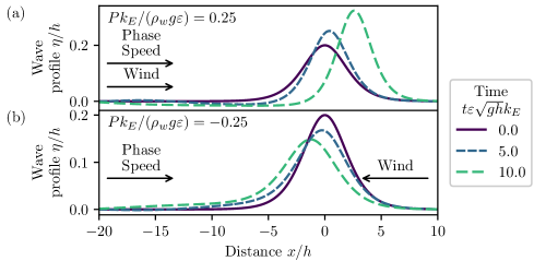
Figure 1: Solitary-wave evolution under 1 onshore and 1 offshore wind-induced surface pressure in the frame of the unforced solitary wave. Non-dimensional wave height $\eta/h$ versus non-dimensional distance $x/h$ for $\varepsilon=0.1$, $\mu_{E}=0.6$, $\absolutevalue{Pk_{E}/(\rho_{w}g\varepsilon)}=0.25$ and non-dimensional slow times $t^{\prime}_{1}=t\varepsilon\sqrt{gh}k_{E}=0$, $5$ and $10$, as indicated in the legend. Only a subset of the full spatial domain is shown. The arrows denote the wave propagation (phase speed) and wind direction.

The wave profile $\eta/h$ snapshots in figure 1 qualitatively show how the wave shape evolves over non-dimensional slow time $t^{\prime}_{1}=t\varepsilon\sqrt{gh}k_{E}$ in the unforced solitary wave’s frame. The onshore wind generates wave growth, apparent at the wave crest (figure 1), whereas the offshore wind causes decay (figure 1). The wind also changes the phase speed, with the wave’s acceleration (deceleration) under an onshore (offshore) wind visible by the advancing (receding) of the crest. This is expected due to the (unforced) solitary wave’s nonlinear phase speed 20 dependence on the wave height $H$.

In shallow water, wave growth/decay and phase speed changes are well-known wind effects (e.g. Miles, 1957; Cavaleri & Rizzoli, 1981), but wind-induced wave shape changes (Zdyrski & Feddersen, 2020) have not been previously studied for shallow-water systems. Such changes are visible in figure 1 where, despite the wave starting from a symmetric, solitary-wave initial condition, the wind induces a horizontal asymmetry in the wave shape, particularly on the rear face ($x<0$) of the wave. The offshore wind (figure 1) raises the rear base of the wave (near $x/h=-5$) relative to its initial profile (purple line), but the onshore wind (figure 1) depresses the rear face and forms a small depression below the still water level at $t\varepsilon\sqrt{gh}k_{E}=5$ (blue line) which widens and deepens at $t\varepsilon\sqrt{gh}k_{E}=10$ (green line). Finally, the onshore wind (figure 1) increases the maximum wave-slope magnitude with time while the offshore wind (figure 1) decreases it, although the windward side of the wave becomes steeper than the leeward side for both winds (up to $8\text{\,}\mathrm{\char 37\relax}$ steeper for the time period shown). Although the equation is ill posed in the sense of Hadamard, the smooth solutions show that our solution is acceptable up to the current time and thus we are justified in neglecting a regularization scheme.

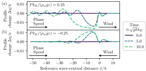
Figure 2: The non-dimensional profile change $\Delta\eta/h$ between the surface profile and reference solitary wave 19 under 2 onshore and 2 offshore Jeffreys forcing versus non-dimensional reference wave-centred distance $\tilde{x}/h$. Results are shown for $\varepsilon=0.1$, $\mu_{E}=0.6$, $\absolutevalue{Pk_{E}/(\rho_{w}g\varepsilon)}=0.25$ and non-dimensional slow times $t^{\prime}_{1}=t\varepsilon\sqrt{gh}k_{E}=0$, $5$ and $10$, as indicated in the legend. Only a subset of the full spatial domain is shown. The arrows denote the direction of wave propagation (phase speed) or wind direction.

To further examine the wind-induced wave asymmetry, we fit $\eta$ to a reference solitary-wave profile $\eta_{\text{ref}}$ 19 by minimizing the $L_{1}$ difference, yielding the reference height $H_{\text{ref}}(t_{1})$ and peak location $x_{\text{ref}}(t_{1})$. The profile change is defined as $\Delta\eta(x)\coloneqq\eta-\eta_{\text{ref}}$ and is shown as a function of the reference wave-centred distance $\tilde{x}\coloneqq x-x_{\text{ref}}$ in figure 2. Notice that the profile change begins near the front face of the wave and has extrema for negative $\tilde{x}^{\prime}$ but with opposite signs for onshore and offshore winds. Additionally, the magnitude of the extrema decay with distance in the $-\tilde{x}$ direction. Finally, note that the onshore (offshore) wind generates a small peak (trough) at $\tilde{x}=0$ and two small troughs (peaks) near $\tilde{x}/h=\pm 3$, with the $\tilde{x}<0$ extrema larger than the $\tilde{x}>0$ one. This is analogous to a dispersive tail, well known in KdV-type systems (e.g. Hammack & Segur, 1974), and its appearance here helps explain the pressure-induced shape change (cf. § 4.2).

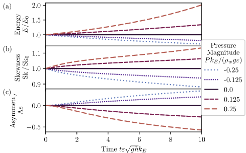
Figure 3: Solitary-wave shape statistics under onshore and offshore Jeffreys forcing versus non-dimensional slow time $t^{\prime}_{1}=t\varepsilon\sqrt{gh}k_{E}=$010$$. The 3 energy (normalized by the initial energy), 3 skewness (normalized by the initial skewness) and 3 asymmetry are defined in 21a–c. Results are shown for $\varepsilon=0.1$, $\mu_{E}=0.6$ and pressure magnitude $\absolutevalue{Pk_{E}/(\rho_{w}g\varepsilon)}$ up to $0.25$, as indicated in the legend. The solid black line is the unforced case, $P=0$, and shows no growth or asymmetry and a constant skewness.

The effect of wind on wave shape is quantified by the time evolution of wave shape statistics — energy, skewness and asymmetry — for onshore and offshore wind (figure 3). We plot all cases for initial steepness $\varepsilon=0.1$ up to slow time $t\varepsilon\sqrt{gh}k_{E}=10$, corresponding to $10/\varepsilon=100$ wave-crossing times, $T_{0}=1/(\sqrt{gh}k_{E})$. The unforced case ($P=0$) displays constant shape statistics and zero asymmetry, as expected. The normalized energy $E/E_{0}$ shows different growth/decay rates: the onshore wind ($P>0$) causes accelerating wave growth while the offshore wind ($P<0$) causes slowing wave decay (figure 3). The energy of the unforced wave is virtually unchanged, with a normalized energy change of $1-E/E_{0}=$-1\text{\times}{10}^{-13}$$ at $t^{\prime}_{1}=10$. The onshore (offshore) wind causes the wave to become more (less) skewed over time, with the normalized skewness nearly symmetric about unity with respect to $\pm P$. Finally, the onshore wind causes a backwards tilt and negative asymmetry while the offshore wind increases the asymmetry and causes a forward tilt, which was also seen in figure 1. Notice that $\absolutevalue{\operatorname{As}}$ is larger for onshore winds than offshore winds. Since the definitions of the skewness and asymmetry are insensitive to waveform scaling $\eta\to\lambda\eta$, this effect is not simply caused by the wave’s growth/decay. Instead, the onshore wind generates a larger dispersive tail (figure 2), which is the asymmetric wave component.

4 Discussion

4.1 Wind speed estimation

We now relate the non-dimensional pressure magnitude $Pk_{E}/(\rho_{w}g)=\order{\varepsilon}$ to the wind speed. First, we need a relationship between the surface pressure and wave energy $E$ 21a–c, which we can approximate using the standard procedure (e.g. Mei, Stiassnie & Yue, 2005) of multiplying the (non-dimensional, denoted by primes) KdV–Burgers equation 18 by $\eta^{\prime}_{0}$ and integrating from $x^{\prime}=-\infty$ to $\infty$ to obtain

$$\partialderivative{t^{\prime}_{1}}\int_{-\infty}^{\infty}{\eta^{\prime}}_{0}^{2}\differential{x^{\prime}}=\int_{-\infty}^{\infty}P^{\prime}\pqty{\partialderivative{\eta^{\prime}_{0}}{x^{\prime}}}^{2}\differential{x^{\prime}}.$$ (22)

The left integral is the non-dimensional energy 21a–c, so re-dimensionalizing and converting back to the full time $t$ gives the energy growth rate $\gamma$,

$$\frac{\gamma}{c_{0}k_{E}}\coloneqq\frac{1}{c_{0}k_{E}E}\partialderivative{E}{t}=\frac{Pk_{E}}{\rho_{w}g}\frac{\langle(\partial_{x}\eta)^{2}\rangle}{\langle(k_{E}\eta)^{2}\rangle}=\frac{1}{5}\frac{Pk_{E}}{\rho_{w}g},$$ (23)

with $\langle(\partial_{x}\eta)^{2}\rangle/\langle(k_{E}\eta)^{2}\rangle=1/5$ evaluated with the initial, solitary-wave profile 19 and the linear, shallow-water phase speed $c_{0}=\sqrt{gh}$ coming from the re-dimensionalization of $t^{\prime}=tc_{0}k_{E}$ 7. Alternatively, a secondary multiple-scale approximation of the forward KdV–Burgers equation has been used previously to derive the energy growth rate for solitary waves as (Zdyrski & McGreevy, 2019)

$$E\propto\frac{1}{\pqty{1-\gamma t}^{2}}\mbox{\quad with\quad}\gamma\coloneqq b\bqty{\frac{Pk_{E}}{\rho_{w}g}}c_{0}k_{E},$$ (24)

with analytically derived $b=2/15$. Numerically fitting 24 to our calculated energy instead yields $b=$0.10081\pm 0.00003$$, similar to the analytic approximation. Note that the exponential energy growth 23 correctly approximates 24 for small times $\gamma t\ll 1$, and both expressions are consistent with the observed accelerating (decelerating) energy change for $P>0$ ($P<0$) in figure 3.

Next, Jeffreys’s (1925) theory relates the growth rate of periodic waves to the wind speed $U_{\lambda/2}$, measured at a height equal to half the wavelength $z=\lambda/2$, as

$$\frac{\gamma}{ck}=S_{\lambda/2}\frac{\rho_{a}}{\rho_{w}}\pqty{\frac{U_{\lambda/2}}{c}-1}\absolutevalue{\frac{U_{\lambda/2}}{c}-1},$$ (25)

with $S_{\lambda/2}$ a small, non-dimensional sheltering parameter potentially dependent on $\varepsilon$, $\mu_{E}$ and $U_{\lambda/2}/c$. For simplicity, we approximate the nonlinear phase speed $c$ (given non-dimensionally in 20) by its leading-order term $c_{0}=\sqrt{gh}$, yielding an error of only $10\text{\,}\mathrm{\char 37\relax}$ in the subsequent calculations. Combining this approximation of 25 with 23 gives

$$U_{\lambda/2}=c_{0}\pqty{1\pm\sqrt{\frac{1}{5}\absolutevalue{\frac{Pk_{E}}{\rho_{w}g}}\frac{\rho_{w}}{\rho_{a}}\frac{1}{S_{\lambda/2}}}}.$$ (26)

Here, the $\pm$ corresponds to onshore ($+$) or offshore ($-$) winds. Note that changing the wind direction (i.e. $\pm$ sign) while holding the surface pressure magnitude $\absolutevalue{Pk_{E}/(\rho_{w}g)}$ constant means onshore wind speeds $\absolutevalue{U_{\lambda/2}}$ will be larger than offshore wind speeds.

We can evaluate 26 for the parameters of § 3: $\varepsilon=0.1$, $\mu_{E}=0.6$ and $Pk/(\rho_{w}g\varepsilon)=0.25$. Donelan et al. (2006) parameterized $S_{\lambda/2}$ for periodic shallow-water waves with a dependence on airflow separation: $S_{\lambda/2}=4.91\varepsilon\sqrt{\mu}$ for our non-separated flow (according to their criterion), with $\mu\coloneqq(kh)^{2}$. Assuming this holds approximately for solitary waves, we choose $\lambda=2\pi/k_{E}=$20\text{\,}\mathrm{m}$$ to calculate the wind speed at $z=\lambda/2=$10\text{\,}\mathrm{m}$$. This choice corresponds to a depth of $h=$2.5\text{\,}\mathrm{m}$$ and initial wave height $H_{0}=$0.5\text{\,}\mathrm{m}$$ and yields a wind speed of $U_{10}=$22\text{\,}\mathrm{m}\text{\,}{\mathrm{s}}^{-1}$$, a physically realistic wind speed for strongly forced shallow-water waves. Weaker wind speeds will induce smaller surface pressures and thus take longer to change the wave shape.

4.2 Physical mechanism of asymmetry generation

Our initial, symmetric solitary waves 19 are permanent-form solutions of the unforced KdV equation. More generally, any initial solitary wave which does not exactly solve the KdV equation will evolve into a solitary wave and a trailing, dispersive tail according to the inverse scattering transform (e.g. Mei, Stiassnie & Yue, 2005). In our system, the pressure continually perturbs the system away from the unforced KdV soliton solution resulting in a trailing, bound, dispersive tail (figure 2), which is responsible for the wave asymmetry. To see this, consider an initial, symmetric profile $\eta$. The pressure forcing term $P\partial_{x}^{2}\eta$ preserves the initial symmetry and induces a symmetric bound wave after a short time $\Delta t^{\prime}_{1}\ll 1$. This is apparent when considering the non-dimensional KdV–Burgers equation 18 in the unforced solitary wave’s frame (figure 1) at the initial time,

$$\evaluated{\partialderivative{\eta^{\prime}_{0}}{t_{1}}}_{t^{\prime}_{1}=0}=-P^{\prime}\partialderivative[2]{x}\bqty{\sech^{2}\pqty{\frac{x^{\prime}}{2}}}$$ (27)

$$\quad\implies\eta^{\prime}_{0}(x^{\prime},\Delta t^{\prime}_{1})=(2-P^{\prime}\Delta t^{\prime}_{1})\sech^{2}\pqty{\frac{x^{\prime}}{2}}+P^{\prime}\Delta t^{\prime}_{1}\frac{3}{2}\sech^{4}\pqty{\frac{x^{\prime}}{2}}.$$ (28)

The $P^{\prime}\Delta t^{\prime}_{1}$ terms generate a small bound wave with a peak (trough) at $x^{\prime}=0$ and troughs (peaks) symmetrically in front and behind the wave peak for onshore (offshore) wind. As time increases, the continual pressure forcing causes the bound wave to grow and lengthen behind the wave, as is apparent in figure 2 (e.g. $\tilde{x}/h=$-203$$ for $P^{\prime}=0.25$ and $t^{\prime}_{1}=10$).

The small numerical value $\absolutevalue{P^{\prime}}=0.25\ll 1$ used in § 3 allows us to consider the wave’s evolution as two steps with time scale separation. First, the pressure generates a bound wave 28 on the slow time scale, and then the wave evolves a dispersive tail on the fast time scale according to the inverse scattering transform of the unforced KdV equation. The dispersive tail in figure 2 (e.g. located left of $\tilde{x}/h=-20$ for $P^{\prime}=0.25$ and $t^{\prime}_{1}=10$) is analogous to the ubiquitous dispersive tails in prior studies on shallow-water solitary waves, such as figures 8(b) and 8(c) of Hammack & Segur (1974). However, unlike dispersive tails generated from initial conditions which fail to satisfy the KdV equation, our tail is continually forced and lengthened by the wind forcing. Finally, interactions with the trailing, dispersive tail are responsible for lengthening the bound wave 28 behind, rather than ahead, of the solitary wave. Hence, the disturbance induced by the pressure forcing 28 has two effects on the wave. First, the wind slowly generates a bound wave which changes the height and width of the initial solitary wave, which is reflected in the growth (decay) and narrowing (widening) under onshore (offshore) winds in figure 1. Second, it quickly generates an asymmetric, dispersive tail behind the wave (figure 2), producing a greater shape change on the wave’s rear face (figure 1). Finally, the different wind directions (i.e. pressure forcing signs) change the sign of the bound wave and dispersive tail and, hence, the sign of the asymmetry in figure 3.

4.3 Comparison to intermediate and deep water

Zdyrski & Feddersen (2020) investigated the effect of wind on Stokes-like waves in intermediate to deep water. This study, with wind coupled to waves in shallow water, finds qualitative agreement with those intermediate- and deep-water results. The shallow-water asymmetry magnitude increases as the pressure magnitude $P$ increases (figure 3), and figure 4(a) of Zdyrski & Feddersen (2020) displayed a similar trend for the corresponding Jeffreys pressure profile, with positive (negative) pressure increasing (decreasing) the asymmetry. Although Zdyrski & Feddersen (2020) compared their theoretical predictions to limited experimental results with $kh>1$, there are no appropriate experiments on wind-induced changes to wave shape in shallow water for comparison with our results. In addition to the Jeffreys pressure profile employed here, Zdyrski & Feddersen (2020) also utilized a generalized Miles profile, only applicable to periodic waves, wherein the pressure was proportional to $\eta$ shifted by a distance parameter $\psi_{P}/k$. Future investigations could couple a higher-order Zakharov equation (e.g. Dommermuth & Yue, 1987) to a Jeffreys-type pressure forcing or to an atmospheric large eddy simulation, as was done for deep water by Hao & Shen (2019). Although this analysis focuses on solitary waves, we also investigated the effect of wind on periodic waves using the cnoidal-wave KdV solutions as initial conditions. Wind-forced cnoidal waves displayed qualitatively similar shape changes with stronger onshore (offshore) wind causing the energy and skewness to increase (decrease) while the asymmetry decreased (increased) with time. Furthermore, results were qualitatively similar across multiple classes of cnoidal waves with different values of $\mu_{E}$, implying that these results apply rather generally.

5 Conclusion

Prior results (Zdyrski & Feddersen, 2020) in intermediate and deep water demonstrated that wind, acting through a wave-dependent surface pressure, can generate shape changes that become more pronounced in shallower water. Here, we produced a novel analysis of wind-induced wave shape changes in shallow water using a multiple-scale analysis to couple weak wind with small, shallow-water waves, i.e. $a_{0}/h\sim(k_{E}h)^{2}\sim Pk/(\rho_{w}g)\ll 1$. This analysis produced a KdV–Burgers equation governing the wave profile $\eta$, which we then solved numerically with a symmetric, solitary-wave initial condition. The deviations between the numerical results and a reference solitary wave had the form of a bound, dispersive tail, with differing signs for onshore and offshore wind. The tail’s presence and shape are the result of a symmetric, pressure-induced shape change evolving under the inverse scattering transform. We also estimated the energy, skewness and asymmetry as functions of time and pressure magnitude. For onshore wind (positive $P$), the wave’s energy and skewness increased with time while asymmetry decreased, while offshore wind produced the opposite effects. Furthermore, these effects were enhanced for strong pressures, and they reduced to the unforced case for $P=0$. The shape statistics found here show qualitative agreement with the results in intermediate and deep water. Finally, the wind speeds corresponding to these pressure differences were calculated and found to be physically realistic.