$hr-$adaptivity for nonconforming high-order meshes with the target matrix optimization paradigm

Abstract

We present an $hr-$adaptivity framework for optimization of high-order meshes. This work extends the $r$-adaptivity method for mesh optimization by Dobrev et al. [1], where we utilized the Target-Matrix Optimization Paradigm (TMOP) to minimize a functional that depends on each element’s current and target geometric parameters: element aspect-ratio, size, skew, and orientation. Since fixed mesh topology limits the ability to achieve the target size and aspect-ratio at each position, in this paper we augment the $r$-adaptivity framework with nonconforming adaptive mesh refinement to further reduce the error with respect to the target geometric parameters. The proposed formulation, referred to as $hr-$adaptivity, introduces TMOP-based quality estimators to satisfy the aspect-ratio-target via anisotropic refinements and size-target via isotropic refinements in each element of the mesh. The methodology presented is purely algebraic, extends to both simplices and hexahedra/quadrilaterals of any order, and supports nonconforming isotropic and anisotropic refinements in 2D and 3D. Using a problem with a known exact solution, we demonstrate the effectiveness of $hr-$adaptivity over both $r-$ and $h-$adaptivity in obtaining similar accuracy in the solution with significantly fewer degrees of freedom. We also present several examples that show that $hr-$adaptivity can help satisfy geometric targets even when $r-$adaptivity fails to do so, due to the topology of the initial mesh.

Article Highlights

• A novel $hr-$adaptivity method is developed for optimizing nonconforming high-order meshes.

• $hr-$adaptivity is more effective in satisfying target geometric parameters of the mesh in comparison to $h-$ and $r-$adaptivity techniques.

• $hr-$adaptivity meshes require fewer degrees of freedom for a given solution accuracy in comparison to $h$- and $r-$adaptivity meshes.

1 Introduction

Mesh quality impacts the fidelity and robustness of the solution of a partial differential equation (PDE) obtained by methods such as the finite element method (FEM), finite volume method (FVM), and the spectral element method (SEM). The quality of a mesh depends on geometrical parameters such as shape and size of each element in the mesh. The ideal values of these parameters depend on factors such as the PDE type, the domain on which the problem is being solved, element types in the mesh (simplices or quadrilaterals/hexahedra), etc. There are three popular approaches for improving the quality of a given mesh without fully reconstructing it, namely, $r-$adaptivity, $h-$adaptivity, and $p-$adaptivity.

The $r-$adaptivity methods move the nodes of the mesh elements without changing the mesh topology. Laplacian smoothing, where each node is typically moved as a linear function of the positions of its neighbors [2, 3, 4], optimization-based smoothing, where a functional based on elements’ geometrical parameters is minimized [5, 6, 7, 8, 9, 10], and equidistribution with respect to an appropriate metric tensor [11, 12] are three popular approaches for $r-$adaptivity. Methods based on $r-$adaptivity enable us to improve the mesh quality to better capture the solution of the PDE of interest. In certain cases, they can also improve the conditioning of the linear system resulting from discretizing the PDE of interest on the given mesh (e.g., [7]). However, there are two key limitations of $r-$adaptivity. First, the effectiveness of $r-$adaptivity methods is restricted by the topology of the given mesh and can fail to achieve the target parameters in the region of interest. Second, once a mesh has been modified by moving its nodal positions, the PDE solution has to be transferred from the original mesh to the improved mesh to continue the PDE solve process. This grid-to-grid transfer can be computationally expensive, especially for high-order discretizations.

In contrast to $r-$adaptivity, $h-$ and $p-$adaptivity based methods do not move the nodal position of the elements, but instead add resolution to the domain by locally refining individual elements of the mesh. In $h-$adaptivity, an element in the mesh can be split into more elements [13], while in $p-$adaptivity, the polynomial order used to represent the solution can be changed in each element to provide more resolution where needed [14]. In each of these approaches, typically an error estimator is employed to determine the elements that should be refined to improve the accuracy of the solution. The advantage of $h-$ and $p-$adaptivity is that each element can be refined to obtain arbitrary resolution in any region of the mesh, irrespective of the shape and size of the original mesh. Additionally, once an element is refined, it is trivial to interpolate the solution from the original element (master) to its refined counterparts (slaves) using interpolation matrices. However, there are two key limitations of $h-$ and $p-$adaptivity. First, these methods cannot control the geometric shape of the mesh elements. Thus, if the error in the solution is due to the skewness or orientation of the element (e.g., magnetohydrodynamic applications), $h$- or $p$-adaptivity methods cannot be used to produce arbitrary accuracy in the solution. Second, as each element is refined to increase the resolution in the domain, the computational cost of the calculation increases.

Based on the advantages and disadvantages of each method, a combination of $r-$adaptivity with $h-$ and/or $p-$adaptivity can help circumvent the shortcomings of each of these individual methods. In this work, we focus on $hr-$adaptivity; $r\!p-$ and $hr\!p-$adaptivity will be explored in future papers. A survey of the literature shows that $hr-$adaptivity methods have been effective for mesh optimization with applications ranging from the Schrödinger equations [15] to ocean modeling [16]. These methods typically employ an error-based function that is minimized by moving the nodal positions ($r-$adaptivity) followed by refining/derefining each element ($h-$adaptivity) by elemental operations such as node insertion, node removal, or edge swapping. A non-exhaustive list of publications and recent advances on the subject of $hr-$adaptivity is given by [15, 16, 17, 18, 19, 20, 21, 22, 23, 24]. All of the existing methods $hr-$ methods are either restricted to low-order meshes (first- or second-order), specific element types (simplices or quadrilaterals/hexahedra), or specific $h-$refinement types (typically isotropic).

In this work, we present a high-order $hr-$adaptivity method based on the Target-Matrix Optimization Paradigm (TMOP). The algorithm is applicable to curved meshes of any order. It supports isotropic refinements for simplices, and both isotropic and anisotropic anisotropic refinements for quadrilaterals/hexahedra, leading to nonconforming 2D and 3D meshes with hanging nodes. This paper demonstrates that TMOP can be used in $hr-$adaptivity settings to adapt the shape and size of the mesh elements, and ultimately improve the accuracy, compared to standalone $h-$adaptivity and $r-$adaptivity, with which the solution of a PDE can be represented on the given mesh.

The rest of the paper is organized as follows. In Section 2 we review TMOP for $r-$adaptivity [1] and the adaptive mesh refinement framework ($h-$adaptivity) [13] that are the starting points of this work. In Section 3 we describe how we integrate the $h-$adaptivity framework with TMOP to construct a novel $hr-$adaptivity technique. Finally, we present several numerical experiments in Section 4 that show the effectiveness of our framework in improving the computational efficiency and accuracy of the numerical solution in comparison to $h-$adaptivity and $r-$adaptivity. Conclusions are presented in Section 5.

2 Overview of TMOP, $r-$adaptivity and $h-$adaptivity

This section provides a basic description of the $r-$adaptivity and $h-$adaptivity algorithms that are the starting point of this work. We only focus on the aspects that are relevant to the final $hr-$adaptivity method.

2.1 Discrete mesh representation

In our finite element based framework, the domain $\Omega\in\mathbb{R}^{d}$ is discretized as a union of curved mesh elements of order $k$. To obtain a discrete representation of these elements, we select a set of scalar basis functions $\{\bar{w}_{i}\}_{i=1}^{N_{w}}$ on the reference element $\bar{E}$. This basis spans the space of all polynomials of degree at most $k$ on the given element type (quadrilateral, tetrahedron, etc.). The position of an element $E$ in the mesh $\mathcal{M}$ is fully described by a matrix $\mathbf{x}_{E}$ of size $d\times N_{w}$ whose columns represent the coordinates of the element control points (a.k.a. nodes or element degrees of freedom). Given $\mathbf{x}_{E}$, we introduce the map $\Phi_{E}:\bar{E}\to\mathbb{R}^{d}$ whose image is the element $E$:

$$x(\bar{x})=\Phi_{E}(\bar{x})\equiv\sum_{i=1}^{N_{w}}\mathbf{x}_{E,i}\bar{w}_{i}(\bar{x})\,,\qquad\bar{x}\in\bar{E},$$ (1)

where we used $\mathbf{x}_{E,i}$ to denote the $i$-th column of $\mathbf{x}_{E}$, i.e., the $i-$th degree of freedom of element $E$. To ensure continuity between mesh elements, we define a global vector $\mathbf{x}$ of mesh positions that contains the $\mathbf{x}_{E}$ control points for every element.

2.2 TMOP for $r-$adaptivity

The objective of the $r-$adaptivity process is to optimize the mesh using information from a discrete function, e.g., a finite element solution function that is defined with respect to the initial mesh. In TMOP, $r-$adaptivity is achieved by incorporating the discrete data into the target geometrical configuration. In this subsection we summarize the main components of the TMOP approach; all details of the specific method we use are provided in [1].

The major concept of TMOP is the user-specified transformation ($W$), from reference-space to target coordinates, which represents the ideal geometric properties of every mesh point. The construction of this transformation is guided by the fact that any Jacobian matrix can be written as a combination of four components:

$$W=\underbrace{\zeta}_{\text{[volume]}}\underbrace{R}_{\text{[rotation]}}\underbrace{Q}_{\text{[skewness]}}\underbrace{D}_{\text{[aspect-ratio]}}.$$ (2)

Further details about this decomposition and a thorough discussion on how TMOP’s target construction methods encode geometric information into the target matrix $W$ is given by Knupp in [25]. For $r-$adaptivity in PDE-based applications, the geometric parameters of (2) are typically constructed as discrete functions using the discrete solution available on the initial mesh. As the nodal coordinates change during $r-$adaptivity, the discrete functions have to be mapped from the original mesh to the updated mesh to ensure that $W$ can be constructed at each reference point, see Section 4 in [26].

Using (1), the Jacobian of the mapping $\Phi_{E}$ at any reference point $\bar{{\bf x}}\in\bar{E}$ from the reference-space coordinates to the current physical-space coordinates is defined as

$$A(\bar{{\bf x}})=\frac{\partial\Phi_{E}}{\partial\bar{{\bf x}}}=\sum_{i=1}^{N_{w}}\mathbf{{\bf x}}_{E,i}[\nabla\bar{w}_{i}(\bar{{\bf x}})]^{T}\,.$$ (3)

Figure 1: Schematic representation of the major TMOP matrices.

Combining (3) and (2), the transformation from the target coordinates to the current physical coordinates (see Fig. 1) is defined as

$$T=AW^{-1}.$$ (4)

With the transformation $T$, a quality metric $\mu(T)$ is used to measure the difference between $A$ and $W$ in terms of the geometric parameters of interest specified in (2). For example, $\mu_{2}=\mid T\mid^{2}/2\tau-1$ is a shape metric that depends on the skew and aspect ratio components, but is invariant to orientation and volume. Here, $\mid T\mid$ is the Frobenius norm of $T$ and $\tau=\text{det}(T)$. Similarly, $\mu_{55}=(\tau-1)^{2}$ is a size metric that depends only on the volume of the element. We also have shape$+$size metrics such as $\mu_{7}=\mid T-T^{-t}\mid^{2}$ and $\mu_{9}=\tau\mid T-T^{-t}\mid^{2}$ that depend on volume, skew and aspect ratio, but are invariant to orientation.

The quality metric $\mu(T)$ is used for $r-$adaptivity by minimizing the TMOP objective function:

$$F({\bf x})=\sum_{E\in\mathcal{M}}F_{E}({\bf x}_{E})=\sum_{E({\bf x}_{E})}\int_{E_{t}}{\omega}({\bf x})\mu_{i}(T({\bf x}))d{\bf x}_{t},$$ (5)

where $F$ is a sum of the TMOP objective function for each element in the mesh ($F_{E}$), ${\omega}$ is a user-prescribed spatial weight and $E_{t}$ is the target element corresponding to the physical element $E$. In (5), the integral is computed as

$$\sum_{E\in\mathcal{M}}\int_{E_{t}}{\omega}({\bf x}_{t})\mu(T({\bf x}_{t}))d{\bf x}_{t}=\frac{1}{N_{E}}\sum_{E\in\mathcal{M}}\sum_{{\bf x}_{q}\in E_{t}}w_{q}\,\det(W(\bar{{\bf x}}_{q}))\,{\omega}({\bf x}_{q})\mu(T({\bf x}_{q})),$$ (6)

where $\mathcal{M}$ is the current mesh with $N_{E}$ elements, $w_{q}$ are the quadrature weights, and the point $x_{q}$ is the image of the reference quadrature point $\bar{x}_{q}$ in the target element $E_{t}$.

$\begin{array}[]{ccc}\includegraphics[height=130.08731pt]{figures/indicator}&\includegraphics[height=130.08731pt]{figures/indicator_opt}\\ \end{array}$

Figure 2: (left) Material indicator function on the initial uniform mesh and (right) the optimized mesh.

In practice, one may use a combination of multiple metrics with different spatial weights to control different geometric parameters in different regions of the mesh. In that case, the TMOP objective function is defined as a combination of integrals associated with each metric [1]. Using an optimization problem solver (e.g., Newton’s method and L-BFGS), optimum nodal locations can be determined by minimizing the TMOP objective function (5). Figure 2 shows an example of $r-$adaptivity to a discrete material indicator using TMOP to control the aspect-ratio and the size of the elements in a mesh. In this example, the material indicator function is used to define discrete functions for aspect-ratio and size targets in (2), and the mesh is optimized using a shape+size metric.

2.3 Basics of $h-$adaptivity

The $h-$adaptivity component of this work is based on the adaptive mesh refinement framework by Cerveny et al. [13]. Therein, the authors present a highly scalable approach for unstructured nonconforming $h-$adaptivity that can be used for high-order curved meshes consisting of triangles, quadrilaterals, tetrahedra, and hexahedra. The methods support the entire de Rham sequence of finite element spaces, at arbitrarily high-order.

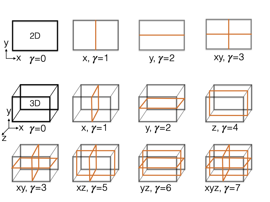
Figure 3: Different refinements options in 2D/3D.

For the purposes of this work, we show all possible refinements for a quadrilateral and a hexahedron element in Figure 3, where we have used $\gamma$ to represent the refinement type. For a hexahedron, $\gamma=1\dots 6$ represent different types of anisotropic refinements and $\gamma=7$ represents isotropic refinement. The $h-$adaptivity framework by Cerveny et al. also supports derefinement where elements introduced by refinement can be removed to restore the parent element that they had originally emanated from. Note that for derefinement, only the elements that share the same parent can be combined together to coarsen the mesh, and a parent can be restored only by coarsening all its children and not a subset thereof. Depending on the specific target, our $hr-$adaptivity method can utilize all different $\gamma$ options for refinement and derefinement.

In practice, an error estimator [27, 28] is used to determine the elements that should be refined or derefined to improve the accuracy of the solution on a given mesh. Figure 4 shows an example of $h-$adaptivity with isotropic and anisotropic refinements based on the spatial gradients of the function. Our $hr-$adaptivity method utilizes a similar approach, where a TMOP-based quality estimator makes refinement and derefinement decisions based on both (i) the function values and (ii) the quality of the mesh.

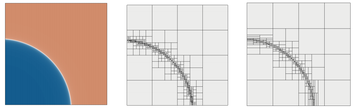
Figure 4: Discrete function in a domain (left) used for $h-$adaptivity with isotropic refinements (center) and anisotropic refinements (right).

3 Methodology for $hr-$adaptivity

In this section we describe our new approach for $hr-$adaptivity, which uses TMOP for $r-$adaptivity as discussed in Section 2.2, and introduces a TMOP-based quality estimator for $h-$adaptivity. The goal of this estimator is to determine the refinement/derefinement decision that minimizes the TMOP objective function $F$, i.e., the difference between the current ($A$) and target ($W$) transformations.

Figure 3 shows how different types of refinement impact the size and aspect-ratio of quadrilaterals and hexahedra. Isotropic refinement of an element reduces its size and anisotropic refinement changes both the aspect-ratio and the size of an element. Thus, $h-$adaptivity can be used with a TMOP-based quality estimator to satisfy the size and aspect-ratio targets in the domain. Note that for curved meshes, $h-$refinement of an element could produce child elements that have different skewness. Example of such configurations can be observed in Figure 5. As described in the following paragraphs, the TMOP-based estimators naturally take into account both the size and the shape changes.

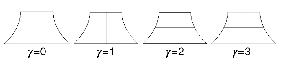
Figure 5: Example of the impact that different types of refinement can have on a high-order curvilinear element in terms of size, aspect-ratio and skewness.

3.1 Refinement decision

Since refining one element does not affect the $A$ matrix of its neighbors, the refinement decision can be performed independently in each element. We define $\Gamma$ as the set of all possible refinements that have to be considered for $h-$adaptivity in a given element. If a size metric is used for the refinement decision, only isotropic refinement is considered. If a shape metric is used, only anisotropic refinements are considered. For a shape+size metric, all refinements are considered. Once $\Gamma$ is constructed, our goal is to find the refinement $\gamma\in\Gamma$ for each element that reduces its TMOP objective function the most:

$$\max_{\gamma}\Delta F^{\gamma}_{E},\,\,\,\gamma\in\Gamma,$$ (7)

where

$$\Delta F^{\gamma}_{E}=F^{\gamma=0}_{E}-\frac{F^{\gamma}_{E}}{N_{c}}.$$ (8)

In (8), the first term on the right hand side denotes the value of the objective function associated with the parent element ($\gamma=0$), and the second term denotes the mean of the objective function associated with the corresponding $N_{c}$ children elements obtained using refinement type $\gamma$ on element $E$:

$$F^{\gamma}_{E}=\sum_{i=1}^{N_{c}}F_{E_{c}}.$$ (9)

If none of the refinements reduce the TMOP objective function for an element, i.e. $\Delta F^{\gamma}_{E}<0\,\,\forall\,\,\gamma$, then that element is not refined.

3.2 Derefinement decision

If the mesh contains children elements, i.e., elements that have been obtained via refinement at a previous iteration of $hr-$adaptivity, we consider them for derefinement if restoring their parent element reduces the TMOP objective function. The derefinement capability is crucial for time-dependent problems where the shape and size targets can change with time as the solution evolves or if the original mesh has more resolution than required to begin with. Using $E_{p}$ to denote a parent element that has been refined to spawn $N_{c}$ children elements at a previous iteration of $hr-$adaptivity, the parent element is derefined if $\Delta F_{E_{p}}>0$, where

$$\Delta F_{E_{p}}=\sum_{i=1}^{N_{c}}\frac{F_{E_{c}}}{N_{c}}-F_{E_{p}}.$$ (10)

As we can see, (8) and (10) are compliments of each other. In (8), we compare how the refinement $\gamma$ changes the TMOP functional between the parent and its children element, and in (10), we see how removing a refinement done using (8) in the past changes the TMOP functional.

3.3 Algorithm for $hr-$adaptivity

The TMOP-based $hr-$adaptivity method is summarized in Algorithm 1. Here, the input consists of the original mesh positions (${\bf x}_{0}$), the mesh quality metric ($\mu$), the tolerance ($\epsilon$) that depends on the norm of the gradient of the TMOP objective function at the current nodal coordinates, and the number of $h-$refinements ($N_{h}$) to be done after each $r-$refinement. The output is the optimized mesh positions ${\bf x}_{s}$. The algorithm performs consecutive $r-$adaptivity and $h-$adaptivity steps until the $h-$adaptivity step does not result in any changes in the mesh output by $r-$adaptivity. Thus, using $N_{R}$ and $N_{D}$ to denote the total number of elements that are refined and derefined, respectively, by the $h-$adaptivity component (Step 6), the $hr-$adaptivity procedure stops when $N_{R}=N_{D}=0$.

Input: ${\bf x}_{0}$, $\mu$, $\epsilon$, $N_{h}$.

Output: ${\bf x}_{s}$ (initialized to ${\bf x}_{0}$).

1 Construct $W_{i}$ for each integration-point $i$ using target-construction.  [25]

2 while $N_{R}\neq 0\,\,{\tt or}\,\,N_{D}\neq 0$ do

3       $r-$adaptivity:

4       ${\bf x}_{s}\rightarrow\underset{{\bf x}}{\operatorname*{arg\,min}}\,\,\,\sum_{E\in\mathcal{M}}\sum_{{\bf x}_{q}\in E_{t}}w_{q}\,\det(W(\bar{{\bf x}}_{q}))\,{\omega}({\bf x}_{q})\mu(T({\bf x}_{q}))$.  [1]

5       $h-$adaptivity:

6       for $i\in 1\dots N_{h}$ do

7             $\forall\,\,\,E_{p}\,\,\,\in\,\,\,\mathcal{M}$, determine $\Delta F_{E_{p}}$.  (10)

8             Derefine element $E_{p}$ if $\Delta F_{E_{p}}>0$.

9             $\forall\,\,\,E\,\,\,\in\,\,\,\mathcal{M}$, determine $\Delta F^{\gamma}_{E}\,\,\,\forall\,\,\,\gamma\,\,\,\in\,\,\,\Gamma$.  (7)

10             Refine element $E$ based on $\max_{\gamma}\Delta F^{\gamma}_{E}$.  [13]

11       end for

12      

13 end while

Algorithm 1 $hr-$adaptivity

In Algorithm 1, determining $\max_{\gamma}\Delta F^{\gamma}_{E}$ requires each element to be refined using each refinement type in $\Gamma$ followed by the targets $W$ and $A$ to be reconstructed on the quadrature points of the children element. This remap of targets from parent to children element is the main source of increase in computational cost for $hr-$adaptivity in comparison to $r-$adaptivity.

The flexibility of the $hr-$adaptivity method can be further increased by utilizing different mesh quality metrics for $r-$adaptivity and $h-$adaptivity in Steps 3 and 5, respectively. This allows us to use different quality metrics to optimize different aspects of the mesh using $h-$adaptivity ($\mu^{h}$) and $r-$adaptivity ($\mu^{r}$). For example, using $\mu^{h}_{2}$ (shape metric) and $\mu^{r}_{7}$ (shape$+$size metric) allows us to optimize the aspect-ratio with $h-$adaptivity, and skew, aspect-ratio and size with $r-$adaptivity.

3.4 Target reconstruction during mesh optimization

For mesh adaptivity, the targets are either defined through analytical functions or through discrete functions that depend on the discrete solution defined on the original mesh. For analytical function based adaptivity, it is straightforward to construct targets at each degree of freedom as the mesh moves during $r-$adaptivity or as new elements are added during $h-$adaptivity. For discrete adaptivity however, the discrete functions must be mapped from the original mesh (${\bf x}_{0}$) to the active mesh (${\bf x}$) so that the targets can be reconstructed to determine $\mu(T)$.

During $r-$adaptivity, the discrete functions are remapped using an advection-based PDE, as described in Section 4.2 of [26], or using high-order interpolation between the meshes (see Section 2.3 of [29]). For $h-$adaptivity, mesh refinement introduces elements that are a subset of existing elements. Since every discrete function defined on the mesh is represented as a polynomial on each element, it is straightforward to interpolate the desired discrete function from a given parent element to its children. The key challenge in mapping the discrete function from the original mesh to the refined mesh is maintaining the desired continuity in the solution at the nonconforming interfaces of the element boundaries. This continuity of the original discrete solution is maintained using a conforming prolongation operator, as described in [13], that extends any function described on the (unconstrained) true degrees of freedom to the (constrained) hanging nodes resulting from refinement operations on the original mesh. Figure 6 shows an example of a nonconforming mesh where isotropic refinement on an element introduces a constrained degree of freedom (labeled “c”) that depends on the true degrees of freedom (labeled “a” and “b”).

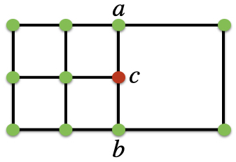
Figure 6: Isotropic refinement of an element in the mesh showing the true degrees of freedom (colored green) and the constrained degree of freedom (labeled “c”). The conforming prolongation operator defines the value at “c” as the average of the values in “a” and “b”.

3.5 Mesh conformity during $r-$adaptivity

An important consideration for the $r-$adaptivity method described in this work is ensuring that the optimal nodal positions determined in Step 3 of Algorithm 1 maintain continuity between the nonconforming interfaces of the mesh.

In our variational formulation (5), the TMOP objective function is computed as an element-by-element weighted sum of the quality metric that measures the deviation between the current and target geometrical parameters of the mesh. Consequently, the derivatives of the TMOP objective function required for $r-$adaptivity are also computed on an element-by-element basis with contribution from each nodal finite element degree of freedom. To maintain continuity between the nonconforming interfaces of the mesh, we project the gradients from the local nodes to the true degrees of freedom using the transpose of the projection operator. Thus, the optimization solver (e.g., Newton’s method) operates on the true degrees of freedom to compute optimum nodal positions, which are used to update the positions of the constrained nodes using the prolongation operator. This approach ensures that the nonconforming interfaces of the mesh stay consistent during nodal movement with $r-$adaptivity.

3.6 Alternative approaches for TMOP estimator during $h-$adaptivity

An alternative to determining how a refinement type changes the TMOP objective function, without explicitly refining each element, is to decompose $A$ into its four geometrical components (e.g., (2)), and then scale the geometrical components based on the refinement type being considered. For example, to estimate how $\gamma=1$ would change the TMOP objective function in a 2D quadrilateral, we take $A$ associated with the quadrature points of the sample point and scale its volume component ($\zeta$) by a factor of 2 to capture the size-reduction and scale the diagonal entries of $D$ to indicate an increase in aspect-ratio in $x$ by a factor of 2. Using this approach, the TMOP estimator becomes:

$$\Delta F^{\gamma}_{E}=F^{\gamma=0}_{E}-\tilde{F}^{\gamma}_{E},$$ (11)

where $\tilde{F}^{\gamma}_{E}$ represents the functional associated with the parent element after the geometrical components of $A$ have been scaled based on $\gamma$. This approach is computationally cheaper than the approach in Algorithm 1 because it does not require each element to be explicitly refined and the targets $W$ to be mapped from the parent element to its children. Numerical experiments show that this approach is as effective as the approach in Algorithm 1 when a low-order mesh is optimized. This behavior is expected because rescaling only the size and aspect-ratio components in (2) to determine the impact of refinement type ignores its impact on the skewness of an element. Since our goal is the optimization of curvilinear high-order meshes, we forego this low-order approach due to higher-accuracy of the approach in Algorithm 1.

Considering the modular structure of the $hr-$adaptivity framework, the TMOP-based estimator for $h-$refinement can also be replaced or used in conjunction with other (error) estimators if desired. All numerical experiments presented in the current work use the TMOP-based estimator.

4 Numerical experiments

In this section, we present several numerical experiments to illustrate the effectiveness of the $hr-$adaptivity method and compare it with standalone $r-$adaptivity and $h-$adaptivity in satisfying the geometric parameters’ targets. The new algorithms were implemented in the open-source MFEM finite element library [30, 31].

4.1 2D benchmark using the Poisson equation

To quantify the improvement in the accuracy of the solution due to $hr-$adaptivity over $r-$adaptivity and $h-$adaptivity, we consider the 2D benchmark from [13] where the Poisson equation with a known exact solution is solved in $\Omega=[0,1]^{2}$,

$$\nabla^{2}u=f.$$ (12)

Here $f$ is chosen such that

$$u=\arctan\bigg{[}\alpha\bigg{(}\sqrt{(x-x_{c})^{2}+(y-y_{c})^{2}}\bigg{)}\bigg{]},$$ (13)

which has a sharp circular wave front of radius $r$ center around $(x_{c},y_{c})$. Figure 7 shows the original second order ($Q_{2}$) mesh with the exact solution for $r=0.7$ and $\alpha=200$. Below we illustrate the effectiveness of different mesh-adaptivity techniques such as $h-$, $r-$, and $hr-$adaptivity in reducing the error in the solution without having to remesh the domain.

$\begin{array}[]{cc}\includegraphics[height=108.405pt]{figures/poisson_original_mesh}&\includegraphics[height=108.405pt]{figures/poisson_solution}\\ \end{array}$

Figure 7: (left) Original $16\times 16$ mesh and (right) the exact solution to the Poisson problem considered here (13).

Since we use a shape+size metric ($\mu_{9}$) to adapt the mesh, the target elements must include information about both shape and size. We use the exact solution to construct the target transformation,

$$W=\sqrt{\zeta}\begin{bmatrix}1&0\\ 0&1\end{bmatrix}\begin{bmatrix}1&\cos\,\phi\\ 0&\sin\,\phi\end{bmatrix}\begin{bmatrix}\frac{1}{\sqrt{\rho}}&0\\ 0&\sqrt{\rho}\end{bmatrix},$$ (14)

where the size target ($\zeta$) depends on the magnitude of the gradient (i.e., $\zeta\propto||\nabla u||$), target skewness ($\phi$) is set to be the same as that for an ideal element, i.e., $\phi=\pi/2$, and aspect ratio target ($\rho$) is computed by the ratio of the gradient components (i.e., $\rho\propto\nabla_{x}u/\nabla_{y}u$). Thus,

$$W=\begin{bmatrix}\sqrt{\frac{\zeta}{\rho}}&0\\ 0&\sqrt{\zeta\rho}\end{bmatrix}.$$ (15)

Figure 8 shows optimized meshes obtained by $h$-, $r$-, and $hr-$adaptivity. The initial mesh for these simulations is the one from Fig. 7. As evident, each of these three methods increases the mesh resolution in the region with sharp solution gradients. While $r-$adaptivity moves nodal positions to increase the resolution, $h-$adaptivity uses anisotropic refinement near the domain boundaries (to satisfy aspect-ratio targets) and isotropic refinement away from the boundaries (to satisfy size targets).

$\begin{array}[]{ccc}\includegraphics[height=108.405pt]{figures/pois_16x16_ha}&\includegraphics[height=108.405pt]{figures/pois_16x16_ra}&\includegraphics[height=108.405pt]{figures/pois_16x16_hra}\\ \end{array}$

Figure 8: Optimized meshes obtained using (left) $h-$adaptivity, (center) $r-$adaptivity, and (right) $hr-$adaptivity.

$\begin{array}[]{c}\includegraphics[height=216.81pt]{figures/hvsrvshr}\\ \end{array}$

Figure 9: Error for the discrete solution ($u_{h}$) with respect to the exact solution ($u$) in the energy norm for a sequence of uniform meshes (the original mesh) and meshes obtained using $h-$adaptivity, $r-$adaptivity, and $hr-$adaptivity.

To obtain a better quantitative comparison, we start with a $4\times 4$ mesh and increase the resolution by a factor of 2 in each direction, while adapting the mesh using $h-$adaptivity, $r-$adaptivity, and $hr-$adaptivity for each case. For $h-$adaptivity we use the same criterion for refinement that is described in Algorithm 1. Additionally, for $h-$adaptivity and $hr-$adaptivity, we consider only 1 iteration of each kind of mesh refinement to illustrate the effectiveness of these methods while keeping the added computational cost to a minimum. Once the mesh has been optimized, the Poisson problem is solved and the error is measured for the discrete solution ($u_{h}$) with respect to the exact solution ($u$) in the energy norm [13]. Figure 9 compares the error for a sequence of uniform meshes (the “original” meshes) with meshes obtained using $h-$adaptivity, $r-$adaptivity, and $hr-$adaptivity. In Fig. 9, $N$ represents the total number of degrees of freedom in the mesh. As evident, $r-$adaptivity can help significantly reduce the error in the solution by moving the nodal positions of the mesh and even a single iteration of $h-$refinement with $hr-$adaptivity is sufficient for an even more significant improvement. This numerical experiment shows that we require about 66% fewer degrees of freedom with $hr-$adaptivity as compared to $r-$adaptivity for a given accuracy in the solution. Note that one can do multiple iterations of $h-$adaptivity and $r-$adaptivity during the mesh-optimization process, but we do a single iteration here to illustrate the effectiveness of these techniques in improving the accuracy of the solution while keeping the computation cost of the mesh-optimization process to a minimum.

4.2 Analytical adaptivity

The next example that we consider is adaptivity based on analytical functions to demonstrate how $hr-$adaptivity can be used for purely size-adaptivity and for shape+size-adaptivity. The $r-$adaptivity component in each case is based on a shape+size metric, and we setup the targets to mimic a problem with a shock wave propagating externally from the center of the domain.

For $hr-$adaptivity with a size metric, the target $W$ is defined in the domain $\Omega\in[0,1]^{2}$ such that the target skewness is the same as that for an ideal element, i.e., $\phi=\pi/2$, target aspect-ratio is unity, i.e. $\rho=1$, and target size ($\zeta$) depends on an analytic function $\eta\in[0,1]$ that is a function of physical-space coordinates (${\bf x}$). Thus,

$$W=\begin{bmatrix}\sqrt{\zeta}&0\\ 0&\sqrt{\zeta}\end{bmatrix},$$ (16)

where

$$\eta=\tanh(\beta(r-0.2))-\tanh(\beta(r-0.3)).$$ (17)

In (17), $\beta$ determines the sharpness in the gradient of the solution, and $r$ is the distance from the center of the domain. Using $\eta$, the size targets are defined as:

$$\zeta=\eta\delta+(1-\eta)\psi\delta,$$ (18)

where $\delta$ is the target size of the degrees of freedom in the region with $\eta=1$ and $\psi$ is the ratio of the biggest to smallest elements in the domain. For the example considered here, we set $\beta=30$, $\delta=0.001$, and $\psi=10$.

$\begin{array}[]{cccc}\includegraphics[height=71.13188pt]{figures/app1_coarse_grid+metric}&\includegraphics[height=71.13188pt]{figures/app1_coarse_h}&\includegraphics[height=71.13188pt]{figures/app1_coarse_r}&\includegraphics[height=71.13188pt]{figures/app1_coarse_hr}\\ \lx@intercol\hfil\textrm{(i) $8\times 8$ mesh}\hfil\lx@intercol\\ \includegraphics[height=71.13188pt]{figures/app1_fine_grid+metric}&\includegraphics[height=71.13188pt]{figures/app1_fine_h}&\includegraphics[height=71.13188pt]{figures/app1_fine_r}&\includegraphics[height=71.13188pt]{figures/app1_fine_hr}\\ \lx@intercol\hfil\textrm{(ii) $16\times 16$ mesh}\hfil\lx@intercol\end{array}$

Figure 10: Analytic size target for optimizing (i) $8\times 8$ and (ii) $16\times 16$ meshes with equally sized elements. In each case, we show (left to right) (a) the original mesh with metric values $\mu^{r}(T)$ compared with meshes obtained using (b) $h-$adaptivity, (c) $r-$adaptivity, and (d) $hr-$adaptivity.

Figure 10 shows examples of the difference in the optimized meshes obtained using $hr-$adaptivity ($\mu^{h}_{55}$ and $\mu^{r}_{7}$) versus $r-$adaptivity ($\mu^{r}_{7}$) and $h-$adaptivity-only ($\mu^{h}_{55}$) for two different initial mesh resolutions. For each case, the left panel shows the quality metric $\mu^{r}_{7}(T)$ evaluated at the degrees of freedom of the original mesh, which indicates the difference between the current and the target geometric parameters (16). For the mesh with $N_{E}=64$ equally sized elements, $h-$adaptivity reduces the TMOP objective function $F({\bf x})$ by 40.36% while increasing the element count to $N_{E}=484$, $r-$adaptivity does not reduce $F({\bf x})$, and $hr-$adaptivity reduces $F({\bf x})$ by 69.2% while increasing the element count to $N_{E}=616$. For the $16\times 16$ mesh, $h-$adaptivity reduces $F({\bf x})$ by 21.9% with $N_{E}=544$, $r-$adaptivity reduces $F({\bf x})$ by 51.8%, and $hr-$adaptivity reduces $F({\bf x})$ by 67.3% with $N_{E}=616$.

$\begin{array}[]{cccc}\includegraphics[height=71.13188pt]{figures/app1_coarse_grid+metric}&\includegraphics[height=71.13188pt]{figures/app2_coarse_h}&\includegraphics[height=71.13188pt]{figures/app2_coarse_r}&\includegraphics[height=71.13188pt]{figures/app2_coarse_hr}\\ \lx@intercol\hfil\textrm{(i) $8\times 8$ mesh}\hfil\lx@intercol\\ \includegraphics[height=71.13188pt]{figures/app1_fine_grid+metric}&\includegraphics[height=71.13188pt]{figures/app2_fine_h}&\includegraphics[height=71.13188pt]{figures/app2_fine_r}&\includegraphics[height=71.13188pt]{figures/app2_fine_hr}\\ \lx@intercol\hfil\textrm{(ii) $16\times 16$ mesh}\hfil\lx@intercol\end{array}$

Figure 11: Analytic shape+size target for optimizing (i) $8\times 8$ and (ii) $16\times 16$ meshes with equally sized elements. In each case, we show (left to right) (a) the original mesh with metric values $\mu^{r}(T)$ compared with meshes obtained using (b) $h-$adaptivity, (c) $r-$adaptivity, and (d) $hr-$adaptivity.

For $hr-$adaptivity with a shape+size metric ($\mu^{h}_{7}$), we modify the target ($W$) such that the aspect-ratio depends on the distance from the center ($r$) and the angle around the center of the domain, i.e., $\rho=f(r,\theta)$. Figure 11 shows that $hr-$adaptivity is able to optimize the mesh and satisfy the shape+size targets much better as compared to $r-$adaptivity. For the $8\times 8$ mesh, $h-$adaptivity reduces $F({\bf x})$ by 92.7% with a final element count of $N_{E}=572$, $r-$adaptivity reduces $F({\bf x})$ by 6.1%, and $hr-$adaptivity reduces $F({\bf x})$ by 93.5% with $N_{E}=704$. For the $16\times 16$ mesh, $F({\bf x})$ is reduced 65.6% by $h-$adaptivity, 60.6% by $r-$adaptivity, and 85.3% by $hr-$adaptivity, with $N_{E}=600$ for $h-$adaptivity and $N_{E}=716$ for $hr-$adaptivity.

4.3 Mesh adaptivity with simplices

The $hr-$adaptivity method described in this paper extends to simplices, where the refinements are always isotropic. So far, we have looked at examples with structured quadrilateral meshes. Due to the ease with which more general domains can be meshed with simplices, however, triangles/tetrahedra are often preferred over quadrilaterals/hexahedra in complicated domains.

$\begin{array}[]{cccc}\includegraphics[height=99.58464pt]{figures/app3_grid+metric}&\includegraphics[height=99.58464pt]{figures/app3_h}&\includegraphics[height=99.58464pt]{figures/app3_r}&\includegraphics[height=99.58464pt]{figures/app3_hr}\end{array}$

Figure 12: Adaptivity on simplices: (left to right) (a) original mesh compared with the optimized mesh using (b) $h-$adaptivity, (c) $r-$adaptivity, and (d) $hr-$adaptivity.

Figure 12 shows an example of a mesh ($N_{E}=128$) with simplices optimized using $h-$adaptivity, $r-$adaptivity and $hr-$adaptivity with $\mu_{9}^{r}$ and $\mu_{55}^{h}$ using the targets in (16). For this example, $F({\bf x})$ is reduced 62.4% by $h-$adaptivity, 43.9% by $r-$adaptivity, and 85.2% by $hr-$adaptivity, while the total element count is increased to $N_{E}=928$ by $h-$adaptivity and to $N_{E}=1100$ by $hr-$adaptivity. Note that while the final element count is significantly higher for the examples in Fig. 10-12 for $hr-$adaptivity in comparison to $r-$adaptivity, that is expected due to the target size and aspect-ratio. Additionally, as we have demonstrated in Fig. 9, the total number of degrees of freedom required for a desired accuracy in solution is typically lower for meshes obtained with $hr-$adaptivity as compared to $r-$adaptivity and $h-$adaptivity.

4.4 Mesh adaptivity with derefinement

The examples in the previous sections demonstrate that the ability of adding elements with $hr-$adaptivity can be critical for satisfying size and aspect-ratio adaptivity targets, depending on the topology, size, and shape of the elements in the original mesh. For time-dependent problems however, where the need for spatial resolution changes with time, the ability to remove elements (i.e, derefinement) is also critically important for maximizing the computational efficiency of a calculation.

$\begin{array}[]{ccc}\includegraphics[height=99.58464pt]{figures/app4_grid+metric}&\includegraphics[height=99.58464pt]{figures/app4_r}&\includegraphics[height=99.58464pt]{figures/app4_hr}\\ \end{array}$

Figure 13: Adaptivity with derefinement: (left) original mesh compared with the optimized mesh using (center) $r-$adaptivityand (right) $hr-$adaptivity.

Here, we consider the example from Section 4.2 where we optimize the mesh using $\mu_{9}^{r}$ and $\mu^{h}_{55}$ with the targets (16). We start with a $4\times 4$ mesh and isotropically refine each element four times, to obtain a mesh with $N_{E}=4096$ elements. As a result, the final mesh has many more elements than required. In contrast to Fig. 10, where the mesh was much coarser and the resulting metric values were highest for the elements in the annulus region with elements larger than specified by $W$, the metric values in Fig. 13 (left panel) are highest for the elements outside the annulus region, as those elements are much smaller than required. With $r-$adaptivity, the element shape and size are optimized to reduce the TMOP objective function by 55.4% but the domain still has more resolution than desired. In contrast, $hr-$adaptivity removes the unneeded resolution by reducing the total element count to $N_{E}=664$, which reduces $F({\bf x})$ by 98.6%.

4.5 2D and 3D $hr-$adaptivity in ALE hydrodynamics

In this section, we consider a 2D and a 3D test case for $hr-$adaptivity in the context of Arbitrary Lagrangian-Eulerian (ALE) hydrodynamics. The 2D case represents a high velocity impact of gasses that was originally proposed in [32]. It involves three materials that represent an impactor, a wall, and the background. This problem is used to demonstrate the method’s behavior in an impact simulation that cannot be executed in Lagrangian frame to final time as it produces large mesh deformations. The complete thermodynamic setup of this problem and additional details about our multi-material finite element discretization and overall ALE method can be found in [33, 34]. This method is available in a multi-material ALE code where we have integrated the TMOP-based $r-$refinement framework in previous work [1].

To demonstrate the effectiveness of $hr-$adaptivity in capturing the interface of different material regions, we take snapshots of the discrete ALE solution from the gas-impactor test and use these solutions to adapt the corresponding meshes. Following the approach described in Section 4.1, we use the gradient of the discrete density solution to set the size and aspect-ratio targets and then optimize the mesh using $\mu^{r}_{9}$ and $\mu_{1}^{h}$ shape+size metrics.

   

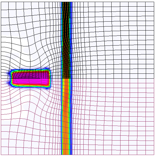
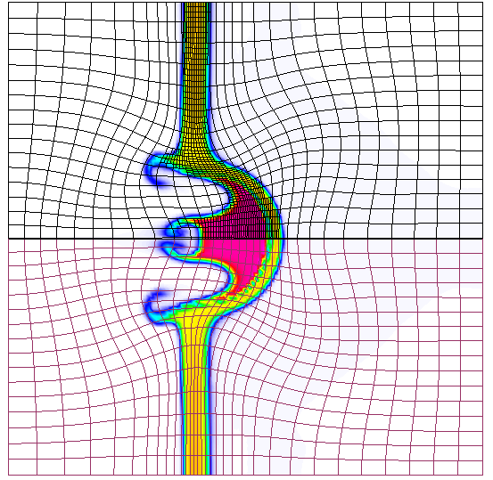
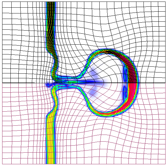
Figure 14: Mesh adaptivity in 2D ALE hydrodynamics: time evolution of density and mesh position at times 0.5 (left), 4 (center) and 9 (right) in the 2D gas impact test case. The meshes obtained with $hr-$adaptivity and $r-$adaptivity are shown in the upper (black) and lower (red) half of the snapshot, respectively. Notice the increased resolution in the wall and the impactor with $hr-$adaptivity.

Figure 14 shows a comparison of the optimized meshes obtained using $r-$ and $hr-$adaptivity along with the density function, before, during, and after the initial impact. These results clearly show that we can achieve a much finer resolution in the regions of interest where different materials are interacting with $hr-$adaptivity as compared to $r-$adaptivity. This example also demonstrates the importance of derefinement, as we can see that the regions that require isotropic and anisotropic refinement are very different at different times.

For the 3D test case, we consider a generalization of the triple point problem in the Lagrangian High-Order Solver (Laghos) miniapp [35], where the domain ($\Omega=[0,7]\times[0,3]\times[0,3]$) is split into 5 different regions with 3 different materials. A complete thermodynamical setup of this problem is discussed in Section 7.4 of [36], and a snapshot of the material regions at simulation time $t=5$ is shown in Fig. 15(a). Since Laghos solves the time-dependent Euler equations in a moving Lagrangian frame of reference, the initial mesh produces no material diffusion. However, in practical simulations, large mesh deformations require ALE methods and mesh optimization. Thus, it is important to be able to adapt the mesh in order to capture curved material interfaces.

$\begin{array}[]{cc}\includegraphics[height=130.08731pt]{figures/triplepoint-laghos}&\includegraphics[height=130.08731pt]{figures/triplepoint-original}\\ \textrm{(a) Material indicator from Laghos.}&\textrm{(b) Uniform hexahedron mesh.}\\ \includegraphics[height=130.08731pt]{figures/triplepoint-r}&\includegraphics[height=130.08731pt]{figures/triplepoint-hr}\\ \textrm{(c) Mesh optimized using $r-$adaptivity.}&\textrm{(d) Mesh optimized using $hr-$adaptivity.}\end{array}$

Figure 15: Mesh adaptivity in 3D ALE hydrodynamics: (a) material indicator function obtained from Laghos is mapped to a (b) uniform hexahedron mesh that is used for mesh optimization. A comparison of the meshes obtained using (c) $r-$adaptivity and (d) $hr-$adaptivity is shown below. Different colors indicate different materials.

For the purposes of this test, we start by transferring the material indicator function defined on the Laghos mesh to a uniform hexahedron mesh (Fig. 15(b)), using a high-order interpolation library [29]. The target shape is set to be the same as that of an ideal element and the target size is computed using the magnitude of the gradient of the material indicator. The $r-$adaptivity component is based on a shape+size metric ($\mu^{r}_{321}$) and the $h-$refinement decisions are made using a size metric ($\mu^{h}_{315}$). Figure 15 shows a comparison of the meshes obtained from $r-$adaptivity and $hr-$adaptivity. While $r-$adaptivity improves the original mesh to align with the original material indicator, its effectiveness in reducing the element size is limited due to the topology of the mesh. In contrast, $hr-$adaptivity allows us to satisfy the size targets by refining the elements that are at the interface of different materials. The uniform hexahedron mesh used here has $N_{E}=896$ elements and $hr-$adaptivity increases the total element count to 3724. To quantify the comparison between these meshes, we look at how well the original material indicator can be represented on each of the meshes in comparison to the mesh from Laghos. Using high-order interpolation, we compute a volumetric error:

$$e=\int_{\Omega}\bigg{(}\eta_{L}({\bf x}_{L})-\eta({\bf x}_{s})\bigg{)}^{2},$$ (19)

that depends on the material indicator $\eta_{L}$ defined on the mesh obtained from Laghos (${\bf x}_{L}$) and the same material indicator function mapped on to the optimized mesh (${\bf x}_{s}$). The volumetric error is 1.71 for the uniform hexahedral mesh, 0.62 for the $r-$adaptivity mesh, and 0.078 for the $hr-$adaptivity mesh. Thus, we see that the volumetric error is almost an order of magnitude lower for the $hr-$adaptivity mesh in comparison to $r-$adaptivity and about $20\times$ lower in comparison to the uniform hexahedron mesh.

The examples presented in this section show the importance of $hr-$adaptivity in the context of complex Lagrangian hydrodynamics applications. In future work, we plan to integrate the $hr-$adaptivity framework in high-order applications with moving meshes to demonstrate the runtime benefits in computational performance.

5 Conclusion

In this paper we presented a new approach for $hr-$adaptivity of high-order meshes. The $r-$adaptivity component of our method is based on the Target Matrix Optimization Paradigm, where the mesh is optimized to minimize a quality metric that depends on the transformation from the current-to-target coordinates. For $h-$adaptivity, we introduced a TMOP-based quality estimator that determines the refinement type (isotropic or anisotropic) on an element-by-element basis to reduce the TMOP objective function. The $hr-$adaptivity procedure uses an iterative loop of $r-$refinements followed by $h-$refinements to adapt the mesh while minimizing the computational cost of the calculation due to increase in the element count. The new $hr-$adaptivity algorithms are freely available in the MFEM finite element library [31]. Numerical experiments show that $hr-$adaptivity helps satisfy the size and aspect-ratio targets where $h-$ and $r-$adaptivity cannot, due to the topology of the input mesh. Using a 2D problem with a known exact solution, we demonstrated that $hr-$adaptivity requires many fewer degrees of freedom for the desired accuracy, in comparison to $h-$ and $r-$adaptivity. We also used several simple 2D problems to demonstrate $hr-$adaptivity for analytic function-based adaptivity in meshes with quadrilaterals and simplices, and the ability to derefine, which is crucial for time-dependent problems where spatial resolution requirements can change with time. Finally, a 2D and a 3D Lagrangian hydrodynamics-based test problems were used to compare the effectiveness of $r-$ with $hr-$refinement in capturing complex curvilinear multi-material interfaces. In the future, we plan to investigate methods for combined $r\!p-$ and $hr\!p-$adaptivity. We will also evaluate the current $hr-$adaptivity framework in applications with high-order moving meshes.

Disclaimer

This document was prepared as an account of work sponsored by an agency of the United States government. Neither the United States government nor Lawrence Livermore National Security, LLC, nor any of their employees makes any warranty, expressed or implied, or assumes any legal liability or responsibility for the accuracy, completeness, or usefulness of any information, apparatus, product, or process disclosed, or represents that its use would not infringe privately owned rights. Reference herein to any specific commercial product, process, or service by trade name, trademark, manufacturer, or otherwise does not necessarily constitute or imply its endorsement, recommendation, or favoring by the United States government or Lawrence Livermore National Security, LLC. The views and opinions of authors expressed herein do not necessarily state or reflect those of the United States government or Lawrence Livermore National Security, LLC, and shall not be used for advertising or product endorsement purposes.

References

- [1] V. A. Dobrev, P. Knupp, T. V. Kolev, K. Mittal, R. N. Rieben, V. Z. Tomov, Simulation-driven optimization of high-order meshes in ALE hydrodynamics, Comput. Fluids (2020).
- [2] J. Vollmer, R. Mencl, H. Mueller, Improved laplacian smoothing of noisy surface meshes, in: Computer graphics forum, Vol. 18, Wiley Online Library, 1999, pp. 131–138.
- [3] D. A. Field, Laplacian smoothing and delaunay triangulations, Communications in applied numerical methods 4 (6) (1988) 709–712.
- [4] G. Taubin, et al., Linear anisotropic mesh filtering, Res. Rep. RC2213 IBM 1 (4) (2001).
- [5] P. Knupp, Introducing the target-matrix paradigm for mesh optimization by node movement, Engr. with Comptr. 28 (4) (2012) 419–429.
- [6] A. Gargallo-Peiró, X. Roca, J. Peraire, J. Sarrate, Optimization of a regularized distortion measure to generate curved high-order unstructured tetrahedral meshes, International Journal for Numerical Methods in Engineering 103 (5) (2015) 342–363.
- [7] K. Mittal, P. Fischer, Mesh smoothing for the spectral element method, Journal of Scientific Computing 78 (2) (2019) 1152–1173.
- [8] V. Dobrev, P. Knupp, T. Kolev, K. Mittal, V. Tomov, The target-matrix optimization paradigm for high-order meshes, SIAM Journal on Scientific Computing 41 (1) (2019) B50–B68.
- [9] P. T. Greene, S. P. Schofield, R. Nourgaliev, Dynamic mesh adaptation for front evolution using discontinuous Galerkin based weighted condition number relaxation, Journal of Computational Physics 335 (2017) 664–687.
- [10] M. Turner, J. Peiró, D. Moxey, Curvilinear mesh generation using a variational framework, Computer-Aided Design 103 (2018) 73–91.
- [11] W. Huang, Y. Ren, R. D. Russell, Moving mesh partial differential equations (MMPDES) based on the equidistribution principle, SIAM J. Numer. Anal. 31 (3) (1994) 709–730.
- [12] W. Huang, R. D. Russell, Adaptive moving mesh methods, Springer Science & Business Media, 2010.
- [13] J. Cerveny, V. Dobrev, T. Kolev, Nonconforming mesh refinement for high-order finite elements, SIAM Journal on Scientific Computing 41 (4) (2019) C367–C392.
- [14] F. Barros, S. Proença, C. de Barcellos, On error estimator and p-adaptivity in the generalized finite element method, International Journal for Numerical Methods in Engineering 60 (14) (2004) 2373–2398.
- [15] J. Mackenzie, W. Mekwi, An hr-adaptive method for the cubic nonlinear schrödinger equation, Journal of Computational and Applied Mathematics 364 (2020) 112320.
- [16] M. Piggott, C. Pain, G. Gorman, P. Power, A. Goddard, h, r, and hr adaptivity with applications in numerical ocean modelling, Ocean modelling 10 (1-2) (2005) 95–113.
- [17] H. Jahandari, S. MacLachlan, R. D. Haynes, N. Madden, Finite element modelling of geophysical electromagnetic data with goal-oriented hr-adaptivity, Computational Geosciences 24 (2020) 1257–1283.
- [18] M. Piggott, P. Farrell, C. Wilson, G. Gorman, C. Pain, Anisotropic mesh adaptivity for multi-scale ocean modelling, Philosophical Transactions of the Royal Society A: Mathematical, Physical and Engineering Sciences 367 (1907) (2009) 4591–4611.
- [19] B. Ong, R. Russell, S. Ruuth, An hr moving mesh method for one-dimensional time-dependent pdes, in: Proceedings of the 21st International Meshing Roundtable, Springer, 2013, pp. 39–54.
- [20] P. Mostaghimi, J. R. Percival, D. Pavlidis, R. J. Ferrier, J. L. Gomes, G. J. Gorman, M. D. Jackson, S. J. Neethling, C. C. Pain, Anisotropic mesh adaptivity and control volume finite element methods for numerical simulation of multiphase flow in porous media, Mathematical Geosciences 47 (4) (2015) 417–440.
- [21] M. Piggott, G. Gorman, C. Pain, P. Allison, A. Candy, B. Martin, M. Wells, A new computational framework for multi-scale ocean modelling based on adapting unstructured meshes, International Journal for Numerical Methods in Fluids 56 (8) (2008) 1003–1015.
- [22] M. Walkley, P. K. Jimack, M. Berzins, Anisotropic adaptivity for the finite element solutions of three-dimensional convection-dominated problems, International journal for numerical methods in fluids 40 (3-4) (2002) 551–559.
- [23] P. F. Antonietti, P. Houston, An hr-adaptive discontinuous galerkin method for advection-diffusion problems, in: Communications to SIMAI congress, Vol. 3, 2020.
- [24] M. G. Edwards, J. T. Oden, L. Demkowicz, An h-r-adaptive approximate riemann solver for the euler equations in two dimensions, SIAM Journal on scientific computing 14 (1) (1993) 185–217.
- [25] P. Knupp, Target formulation and construction in mesh quality improvement, Tech. Rep. LLNL-TR-795097, Lawrence Livermore National Lab.(LLNL), Livermore, CA (United States) (2019).
- [26] V. A. Dobrev, P. Knupp, T. V. Kolev, V. Z. Tomov, Towards Simulation-Driven Optimization of High-Order Meshes by the Target-Matrix Optimization Paradigm, Springer International Publishing, 2019, pp. 285–302.
- [27] I. Babuska, W. C. Rheinboldt, Reliable error estimation and mesh adaptation for the finite element method., Tech. rep., Maryland Univ College Park Inst For Physical Science And Technology (1979).
- [28] M. Ainsworth, J. T. Oden, A posteriori error estimation in finite element analysis, Vol. 37, John Wiley & Sons, 2011.
- [29] K. Mittal, S. Dutta, P. Fischer, Nonconforming Schwarz-spectral element methods for incompressible flow, Computers & Fluids 191 (2019) 104237.
- [30] R. Anderson, J. Andrej, A. Barker, J. Bramwell, J.-S. Camier, J. C. V. Dobrev, Y. Dudouit, A. Fisher, T. Kolev, W. Pazner, M. Stowell, V. Tomov, I. Akkerman, J. Dahm, D. Medina, S. Zampini, MFEM: A modular finite element library, Computers & Mathematics with Applications (2020). doi:10.1016/j.camwa.2020.06.009.
- [31] MFEM: Modular finite element methods [Software], https://mfem.org. doi:10.11578/dc.20171025.1248.
- [32] A. Barlow, R. Hill, M. J. Shashkov, Constrained optimization framework for interface-aware sub-scale dynamics closure model for multimaterial cells in Lagrangian and arbitrary Lagrangian-Eulerian hydrodynamics, J. Comput. Phys. 276 (0) (2014) 92–135.
- [33] V. A. Dobrev, T. V. Kolev, R. N. Rieben, V. Z. Tomov, Multi-material closure model for high-order finite element Lagrangian hydrodynamics, Int. J. Numer. Meth. Fluids 82 (10) (2016) 689–706.
- [34] R. W. Anderson, V. A. Dobrev, T. V. Kolev, R. N. Rieben, V. Z. Tomov, High-order multi-material ALE hydrodynamics, SIAM J. Sci. Comp. 40 (1) (2018) B32–B58.
- [35] Laghos: High-order Lagrangian hydrodynamics miniapp [Software], https://github.com/ceed/Laghos (2020).
- [36] X. Zeng, G. Scovazzi, A variational multiscale finite element method for monolithic ale computations of shock hydrodynamics using nodal elements, Journal of Computational Physics 315 (2016) 577–608.