Knowledge Association with Hyperbolic Knowledge Graph Embeddings

Abstract

Capturing associations for knowledge graphs (KGs) through entity alignment, entity type inference and other related tasks benefits NLP applications with comprehensive knowledge representations. Recent related methods built on Euclidean embeddings are challenged by the hierarchical structures and different scales of KGs. They also depend on high embedding dimensions to realize enough expressiveness. Differently, we explore with low-dimensional hyperbolic embeddings for knowledge association. We propose a hyperbolic relational graph neural network for KG embedding and capture knowledge associations with a hyperbolic transformation. Extensive experiments on entity alignment and type inference demonstrate the effectiveness and efficiency of our method.

1 Introduction

Knowledge graphs (KGs) have emerged as the driving force of many NLP applications, e.g., KBQA Hixon et al. (2015), dialogue generation Moon et al. (2019) and narrative prediction Chen et al. (2019). Different KGs are usually extracted from separate data sources or contributed by people with different expertise. Therefore, it is natural for these KGs to constitute complementary knowledge of the world that can be expressed in different languages, structures and levels of specificity Lehmann et al. (2015); Speer et al. (2017). Associating multiple KGs via entity alignment Chen et al. (2017) or type inference Hao et al. (2019) particularly provides downstream applications with more comprehensive knowledge representations.

Entity alignment and type inference seek to find two kinds of knowledge associations, i.e., sameAs and instanceOf, respectively. An example showing such associations is given in Figure 1. Specifically, entity alignment is to find equivalent entities from different entity-level KGs, such as United States in DBpedia and United States of America in Wikidata. Type inference, on the other hand, associates a specific entity with a concept describing its type information, such as United States and Country. The main difference lies in whether such knowledge associations express the same level of specificity or not. Challenged by the diverse schemata, relational structures and granularities of knowledge representations in different KGs Nikolov et al. (2009), traditional symbolic methods usually fall short of supporting heterogeneous knowledge association Suchanek et al. (2011); Lacoste-Julien et al. (2013); Paulheim and Bizer (2013). Recently, increasing efforts have been put into exploring embedding-based methods Chen et al. (2017); Trivedi et al. (2018); Jin et al. (2019). Such methods capture the associations of entities or concepts in a vector space, which can help overcome the symbolic and schematic heterogeneity Sun et al. (2017).

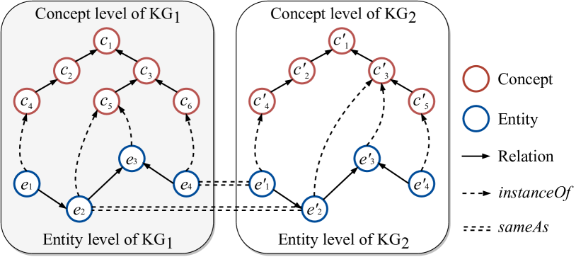
Figure 1: Illustration of two kinds of knowledge associations (i.e., sameAs and instanceOf) in KGs.

Embedding-based knowledge association methods still face challenges in the following aspects. (i) Hierarchical structures. A KG usually consists of many local hierarchical structures Hu et al. (2015). Besides, a KG also usually comes with an ontology to manage the relations (e.g., subClassOf) of concepts Hao et al. (2019), which typically forms hierarchical structures as illustrated in Figure 1. It is particularly difficult to preserve such hierarchical structures in a linear embedding space Nickel et al. (2014). (ii) High parameter complexity. To enhance the expressiveness of KG embeddings, many methods require high embedding dimensions, which inevitably cause excessive memory consumption and intractable parameter complexity. For example, for the entity alignment method GCN-Align Wang et al. (2018), the embedding dimension is selected to be as large as $1,000$. Reducing the dimensions can effectively decrease memory cost and training time. (iii) Different scales. The KGs that we manipulate may differ in scales. For example, while the English DBpedia contains $4,233,000$ entities, its ontology only contains less than a thousand concepts. Capturing the associations between entities and concepts has to deal with drastically different scales of structures and search spaces, while most existing methods do not consider such difference.

To tackle these challenges, we propose a novel hyperbolic knowledge association method, namely HyperKA, inspired by the recent success of hyperbolic representation learning Nickel and Kiela (2017); Dhingra et al. (2018); Tifrea et al. (2019). Unlike the Euclidean circle circumference that grows linearly w.r.t. the radius, the hyperbolic space grows exponentially with the radius. This property makes the hyperbolic geometry particularly suitable for embedding the hierarchical structures that drastically span their sizes along with their levels. It is also capable of achieving superior expressiveness at a low dimension. To leverage such merit, HyperKA employs a hyperbolic relational graph neural network (GNN) for KG embedding and captures multi-granular knowledge associations with a hyperbolic transformation between embedding spaces. For each KG, HyperKA first incorporates hyperbolic translational embeddings at the input layer of the GNN. Then, several hyperbolic graph convolution layers are stacked over the inputs to aggregate neighborhood information and obtain the final embeddings of entities or concepts. On top of the KG embeddings, a hyperbolic transformation is jointly trained to capture the associations. We conduct extensive experiments on entity alignment and type inference. HyperKA outperforms SOTA methods on both tasks at a moderate dimension (e.g., $50$ or $75$). Even with a small dimension (e.g., $10$), our method still shows competitive performance.

2 Background

2.1 Knowledge Association

Knowledge association aims at capturing the correspondence between structured knowledge that is described under the same or different specificity. In this paper, we consider two knowledge association tasks, i.e., entity alignment between two entity-level KGs and type inference from an entity-level KG to an ontological one. We define a KG as a 3-tuple $\mathcal{K}=\{\mathcal{E},\mathcal{R},\mathcal{T}\}$, where $\mathcal{E}$ denotes the set of objects such as entities or concepts. $\mathcal{R}$ denotes the set of relations and $\mathcal{T}\subseteq\mathcal{E}\times\mathcal{R}\times\mathcal{E}$ denotes the set of triples. Each triple $\tau=(h,r,t)$ records a relation $r$ between the head and tail objects $h$ and $t$. On top of this, the associations between two entity-level KGs (or between one entity-level and one ontological KGs) $\mathcal{K}_{1}=\{\mathcal{E}_{1},\mathcal{R}_{1},\mathcal{T}_{1}\}$ and $\mathcal{K}_{2}=\{\mathcal{E}_{2},\mathcal{R}_{2},\mathcal{T}_{2}\}$ are defined as $\mathcal{A}=\{(i,j)\in\mathcal{E}_{1}\times\mathcal{E}_{2}\,|\,i\to j\}$, where $\to$ denotes a kind of associations, such as the sameAs relationship for entity alignment or the instanceOf relationship in the case of type inference. A small subset of associations $\mathcal{A}^{+}\subset\mathcal{A}$ are usually given as training data and we aim at finding the remaining.

2.2 Related Work

Knowledge association tasks and methods. Entity alignment or type inference between KGs can be viewed as a knowledge association task. A typical method of entity alignment is MTransE Chen et al. (2017). It jointly conducts translational embedding learning Bordes et al. (2013) and alignment learning to capture the matches of entities based on embedding distances or transformations. As for type inference, JOIE Hao et al. (2019) deploys a similar framework to learn associations between entities and concepts. Later studies explore with three lines of techniques for improvement. (i) KG embedding. Besides translational embeddings, some studies employ other relational learning techniques such as circular correlations Hao et al. (2019); Shi and Xiao (2019), recurrent skipping networks Guo et al. (2019), and adversarial learning Pei et al. (2019a, b); Lin et al. (2019). Others employ various GNNs to seize the relatedness of entities based on neighborhood information, including GCN Wang et al. (2018); Cao et al. (2019), GAT Zhu et al. (2019); Li et al. (2019); Mao et al. (2020) and relational GCNs Wu et al. (2019a, b); Sun et al. (2020a). These techniques seek to better induce embeddings with more comprehensive relational modeling. Other studies for ontology embeddings Lv et al. (2018); Dong et al. (2019) consider relative positions between spheres as the hierarchical relationships of corresponding concepts. However, they are still limited to linear embeddings, hence may easily fall short of preserving the deep hierarchical structures of KGs. (ii) Auxiliary information. Besides relational structures, some studies characterize entities based on auxiliary information, including numerical attributes Sun et al. (2017); Trisedya et al. (2019), literals Gesese et al. (2019); Zhang et al. (2019) and descriptions Yang et al. (2019); Chen et al. (2018); Jin et al. (2019). They capture associations based on alternative resources, but are also challenged by the less availability of auxiliary information in many KGs Speer et al. (2017); Mitchell et al. (2018). (iii) Semi-supervised learning. Another group of studies seek to infer associations with limited supervision, including self-learning Sun et al. (2018, 2019); Zhu et al. (2019) and co-training Chen et al. (2018). These methods are competent in inferring one-to-one entity alignment, without consideration of associations between entities and concepts. A recent survey by Sun et al. (2020b) has systematically summarized all three lines of studies.

Hyperbolic representation learning. Different from Euclidean embeddings, some studies explore to characterize structures in hyperbolic embedding spaces, and use the non-linear hyperbolic distance to capture the relations between objects Nickel and Kiela (2017); Sala et al. (2018). This technique has shown promising performance in embedding hierarchical data, e.g., co-purchase records Vinh et al. (2018), taxonomies Le et al. (2019); Aly et al. (2019) and organizational charts Chen and Quirk (2019). Further work extends hyperbolic embeddings to capture relational hierarchies of sentences Dhingra et al. (2018), neighborhood aggregation Chami et al. (2019); Liu et al. (2019) and missing triples of a KG Kolyvakis et al. (2020); Balazevic et al. (2019). These studies mainly focus on the scenario of a single independent structure. Learning associations across multiple KG structures with hyperbolic embeddings is still an unsolved issue, which is exactly the focus of this paper.

3 Hyperbolic Geometry

The hyperbolic space is one of the three kinds of isotropic spaces. Table 1 lists some key properties of the Euclidean (flat), spherical (positively curved) and hyperbolic (negatively curved) spaces. Compared with the Euclidean and spherical spaces, the amount of space covered by a hyperbolic geometry increases exponentially rather than polynomially w.r.t. the radius. This property allows us to capture KG structures at a very low dimension, and particularly suits those forming hierarchies. For the hyperbolic geometry, there are several important models including the hyperboloid model Reynolds (1993), Klein disk model Nielsen and Nock (2014) and Poincaré ball model Cannon et al. (1997). In this paper, we choose the Poincaré ball model due to its feasibility for gradient optimization Balazevic et al. (2019). Specifically, the $n$-dimensional Poincaré ball with a negative curvature $-c$ ($c>0$) is defined by the manifold $\mathbb{D}^{n,c}=\{x\in\mathbb{R}^{n}\,|\,\|x\|<\frac{1}{c}\}$. For simplicity, we follow Ganea et al. (2018) and let $c=1$. We hereby introduce some basic operations of hyperbolic geometry, which we use extensively.

Euclidean Spherical Hyperbolic Curvature $0$ $>0$ $<0$ Parallel lines $1$ $0$ $\infty$ Shape of triangles Sum of triangle angles $\pi$ $>\pi$ $<\pi$

Table 1: Characteristic properties of Euclidean, spherical and hyperbolic geometries Krioukov et al. (2010).

Hyperbolic distance. The distance between vectors $\mathbf{u}$ and $\mathbf{v}$ in the Poincaré ball is given by:

$$d_{\mathbb{D}}(\mathbf{u},\mathbf{v})=\operatorname{arccosh}(1+2\frac{\|\mathbf{u}-\mathbf{v}\|^{2}}{(1-\|\mathbf{u}\|^{2})(1-\|\mathbf{v}\|^{2})}).$$

When points move from the origin towards the ball boundary, their distance would increase exponentially, offering a much larger volume of space for embedding learning.

Vector translation. The vector translation in the Poincaré ball is defined by the Möbius addition:

$$\mathbf{u}\oplus\mathbf{v}=\frac{(1+2\langle\mathbf{u},\mathbf{v}\rangle+\|\mathbf{v}\|^{2})\mathbf{u}+(1-\|\mathbf{u}\|^{2})\mathbf{v}}{1+2\langle\mathbf{u},\mathbf{v}\rangle+\|\mathbf{u}\|^{2}\|\mathbf{v}\|^{2}}.$$

Transformation. A transformation is the backbone of both GNNs Chami et al. (2019); Liu et al. (2019) and transformation-based associations Chen et al. (2017); Hao et al. (2019). The work in Ganea et al. (2018) defines the matrix-vector multiplication between Poincaré balls using the exponential and logarithmic maps. The hyperbolic vectors are first projected into the tangent space at $\mathbf{0}$ using the logarithmic map ($\log_{\mathbf{0}}:\mathbb{D}^{n,1}\to T_{\mathbf{0},n}\mathbb{D}^{n,1}$), then multiplied the transformation matrix like in the Euclidean space, and finally projected back on the manifold with the exponential map ($\exp_{\mathbf{0}}:T_{\mathbf{0},n}\mathbb{D}^{n,1}\to\mathbb{D}^{n,1}$). Specifically, the two projections on vector $\mathbf{u}\in\mathbb{D}^{n,1}$ are defined as follows:

$$\exp_{\mathbf{0}}(\mathbf{u})=\tanh(\|\mathbf{u}\|)\frac{\mathbf{u}}{\|\mathbf{u}\|},$$ (1)

$$\log_{\mathbf{0}}(\mathbf{u})=\tanh^{-1}(\|\mathbf{u}\|)\frac{\mathbf{u}}{\|\mathbf{u}\|}.$$ (2)

Through such inverse projections, theoretically, we can apply any Euclidean counterpart operations on hyperbolic vectors. The transformation that maps a vector $\mathbf{u}\in\mathbb{D}^{n,c}$ into $\mathbb{D}^{m,c}$ can be done using the Möbius version of matrix-vector multiplication:

$$\mathbf{M}\otimes\mathbf{u}=\exp_{\mathbf{0}}(\mathbf{M}\log_{\mathbf{0}}(\mathbf{u})).$$ (3)

4 Hyperbolic Knowledge Association

In this section, we introduce the technical details of HyperKA — the hyperbolic GNN-based representation learning method for knowledge association. Different from existing relational GNNs like R-GCN Schlichtkrull et al. (2018), AVR-GCN Ye et al. (2019) and CompGCN Vashishth et al. (2020) that perform a relation-specific transformation on relational neighbors before aggregation, our method models relations as translations between entity vectors at the input layer, and performs neighborhood aggregation on top of them to derive the final entity embeddings. This allows our method to benefit from both relation translation and neighborhood aggregation without increasing computation complexity.

4.1 Hyperbolic Relation Translation

Given a triple from the KG, the translational technique Bordes et al. (2013) models a relation as a translation vector between its head and tail entities. This technique has shown promising performance on many downstream tasks such as relation prediction, triple classification and entity alignment Bordes et al. (2013); Chen et al. (2017); Sun et al. (2019). An apparent issue of such translations to embed hierarchies in the Euclidean space is that it would require a large space to preserve the successive relation translations in a hierarchical structure. The data in a hierarchy grows exponentially w.r.t. its levels, while the amount of space grows linearly in a Euclidean space. As a result, the Euclidean embeddings usually come with a high dimension so as to achieve enough expressiveness for the aforementioned hierarchical structures. However, such modeling can be easily done in the hyperbolic space with a low dimension, where the distance between two points increases exponentially as they move towards to the boundary of the hyper-sphere.

In our method, we seek to migrate the original translation operation to the hyperbolic space in a compact way. Accordingly, the following energy function is defined for a triple $\tau=(h,r,t)$:

$$f(\tau)=d_{\mathbb{D}}(\mathbf{u}_{h}^{(0)}\oplus\mathbf{u}_{r}^{(0)},\mathbf{u}_{t}^{(0)}),$$ (4)

where $\mathbf{u}_{h}^{(0)},\mathbf{u}_{r}^{(0)},\mathbf{u}_{t}^{(0)}\in\mathbb{D}^{n,c}$ denote the embeddings for $h$, $r$ and $t$ at the input layer, respectively. Our method is different from some existing methods Balazevic et al. (2019); Kolyvakis et al. (2020) that use hyperbolic relation-specific transformations on entity representations and may easily cause high complexity overhead. The parameter complexity of our translation operation remains the same as TransE. We prefer low energy for positive triples while high energy for negatives. Hence, we minimize the following contrastive learning loss:

$$\mathcal{L}_{\text{rel}}=\sum_{\tau\in\mathcal{T}_{1}\cup\mathcal{T}_{2}}f(\tau)+\sum_{\tau^{\prime}\in\mathcal{T}^{-}}[\lambda_{1}-f(\tau^{\prime})]_{+},$$ (5)

where $\mathcal{T}^{-}$ denotes the set of negative triples generated by corrupting positive triples Sun et al. (2018). $\lambda_{1}$ is the margin where we expect $f(\tau^{\prime})>\lambda_{1}$.

4.2 Hyperbolic Neighborhood Aggregation

GNNs Kipf and Welling (2017) have recently become the paradigm for graph representation learning. Particularly, for the entity alignment task, the main merit of GNN-based methods lies in capturing the high-order proximity of entities based on their neighborhood information Wang et al. (2018). Inspired by the recent proposal of hyperbolic GNNs Liu et al. (2019); Chami et al. (2019), we seek to use the hyperbolic graph convolution to learn embeddings for knowledge association. The typical message passing process of GNNs consists of two phases, i.e., aggregating neighborhood features

$$\mathbf{u}^{(l)}_{\mathcal{N}(i)}=\text{agg}(\{\mathbf{u}^{(l-1)}_{j}|j\in\mathcal{N}(i)\}),$$ (6)

and combining node and neighborhood information

$$\mathbf{u}^{(l)}_{i}=\text{comb}(\mathbf{u}^{(l-1)}_{i},\mathbf{u}^{(l)}_{\mathcal{N}(i)}),$$ (7)

where $\mathbf{u}^{(l)}_{\mathcal{N}(i)}$ denotes the representation of central object $i$ by aggregating its neighborhood information $\mathcal{N}(i)$ at the $l$-th layer. $\mathbf{u}^{(l)}_{i}$ denotes the representation of object $i$ by combining its representation from the last layer $\mathbf{u}^{(l-1)}_{i}$ and the aggregated representation of its neighborhood $\mathbf{u}^{(l)}_{\mathcal{N}(i)}$.

Different aggregation and combination functions lead to different variants of GNNs. We choose the message passing technique that highlights the representations of central objects, to benefit from the translational embeddings at the input layer. Specifically, the message passing process of our hyperbolic GNN from the $(l-1)$-th layer to the $l$-th layer is defined as follows:

$$\mathbf{u}^{(l)}_{i}=\mathbf{u}^{(l-1)}_{i}\oplus\sigma(\mathbf{W}^{(l)}\otimes\mathbf{u}^{(l-1)}_{\mathcal{N}^{\prime}(i)}\oplus\mathbf{b}^{(l)}),$$ (8)

where $\mathbf{W}^{(l)}$ is the transformation matrix and $\mathbf{b}^{(l)}$ is the bias vector at the $l$-th layer. $\sigma$ is an activation function. We adopt mean-pooling to compute $\mathbf{u}^{(l-1)}_{\mathcal{N}^{\prime}(i)}$ based on the representations of entity $i$ and its neighbors from the $(l-1)$-th layer. Generally, we can use the output representation of the final layer $\mathbf{u}_{i}=\mathbf{u}_{i}^{(L)}$ to represent object $i$, where $L$ is the number of GNN layers. To further benefit from relation translation, we can also combine the input and output representations $\mathbf{u}_{i}=\mathbf{u}_{i}^{(0)}\oplus\mathbf{u}_{i}^{(L)}$ as the final embeddings for knowledge association.

4.3 Hyperbolic Knowledge Projection

Once each KG is embedded in a hyperbolic space, the next step is to capture the associations between different KGs. Many previous studies jointly embed different KGs into a unified space Sun et al. (2017); Wang et al. (2018); Li et al. (2019), and infer the associations based on similarity of entity embeddings. However, pursing similar embeddings in a shared space is ill-posed for KGs with inconsistent structures, especially under the cases with different scales of knowledge representations. We hereby tackle the challenge with a knowledge projection technique in the hyperbolic space. Given a pair of seed knowledge association $(i,j)\in\mathcal{A}^{+}$, we use the Möbius multiplication to project $\mathbf{u}_{i}$ to find the target $\mathbf{u}_{j}$ in the other space. The transformation error is defined as the hyperbolic distance between projected embeddings:

$$\pi(i,j)=d_{\mathbb{D}}(\mathbf{M}\otimes\mathbf{u}_{i},\mathbf{u}_{j}),$$ (9)

where $\mathbf{M}\in\mathbb{R}^{n\times m}$ serves as the linear transformation from the hyperbolic space $\mathbb{D}^{n,c}$ of $\mathcal{K}_{1}$ to $\mathbb{D}^{m,c}$ of $\mathcal{K}_{2}$. The two hyperbolic spaces are not necessarily of the same dimension, i.e., we usually have $n\neq m$. The projection loss is defined as follows:

$$\mathcal{L}_{\text{proj}}=\sum_{(i,j)\in\mathcal{A}^{+}}\pi(i,j)+\sum_{(i^{\prime},j^{\prime})\in\mathcal{A}^{-}}[\lambda_{2}-\pi(i^{\prime},j^{\prime})]_{+},$$ (10)

$\mathcal{A}^{-}$ thereof is the set of negative samples of knowledge associations, and $\lambda_{2}>0$ is a margin.

4.4 Training

The overall loss of the proposed method is the combination of relation translation learning and knowledge projection learning, which is given by:

$$\mathcal{L}=\mathcal{L}_{\text{rel}}+\mathcal{L}_{\text{proj}}.$$ (11)

The embedding vectors are initialized using the Xavier normal initializer. Then, we can use the exponential map to project vectors to the Poincaré ball. We adopt the Riemannian SGD algorithm Bonnabel (2013) to optimize the loss function. Let $\mathbf{\theta}$ be the trainable parameters. The Riemannian gradient $\nabla_{\text{H}}$ at $\mathbf{\theta}^{t}$ is computed as follows:

$$\nabla_{\text{H}}=\frac{(1-\|\theta^{t}\|^{2})^{2}}{4}\nabla_{\text{E}},$$ (12)

where $\nabla_{\text{E}}$ denotes the Euclidean gradient. We use Adam Kingma and Ba (2015) as the optimizer.

5 Experiments

We evaluate the proposed method HyperKA on two tasks of knowledge association, i.e. entity alignment (Section 5.1) and entity type inference (Section 5.2). The source code is publicly available.

Methods	Dimensions	ZH-EN			JA-EN			FR-EN
		H@1	H@10	MRR	H@1	H@10	MRR	H@1	H@10	MRR
MTransE Chen et al. (2017)	75	0.308	0.614	0.364	0.279	0.575	0.349	0.244	0.556	0.335
IPTransE Zhu et al. (2017)	75	0.406	0.735	0.516	0.367	0.693	0.474	0.333	0.685	0.451
AlignE Sun et al. (2018)	75	0.472	0.792	0.581	0.448	0.789	0.563	0.481	0.824	0.599
SEA Pei et al. (2019a)	75	0.424	0.796	0.548	0.385	0.783	0.518	0.400	0.797	0.533
RSN4EA Guo et al. (2019)	300	0.508	0.745	0.591	0.507	0.737	0.590	0.516	0.768	0.605
GCN-Align Wang et al. (2018)	1000, 1000, 1000	0.413	0.744	0.549	0.399	0.745	0.546	0.373	0.745	0.532
MuGNN Cao et al. (2019)	128, 128, 128	0.494	0.844	0.611	0.501	0.857	0.621	0.495	0.870	0.621
KECG Li et al. (2019)	128, 128, 128, 128	0.478	0.835	0.598	0.490	0.844	0.610	0.486	0.851	0.610
AliNet Sun et al. (2020a)	500, 400, 300	0.539	0.826	0.628	0.549	0.831	0.645	0.552	0.852	0.657
HyperKA (w/o relation)	75, 75, 75	0.518	0.814	0.623	0.535	0.834	0.640	0.529	0.859	0.645
HyperKA	75, 75, 75	0.572	0.865	0.678	0.564	0.865	0.673	0.597	0.891	0.704

Table 2: Entity alignment results on DBP15K. For the dimension of GNN-based methods, we report the output dimensions of their input layer and GNN layers. The best scores are in bold and the second-best ones are underlined.

5.1 Entity Alignment

Entity alignment aims at matching the counterpart entities that describe the same real-world identity across two entity-level KGs. The inference of entity alignment is based on the embedding distances.

5.1.1 Experimental Setup

Datasets. We use the widely-adopted entity alignment dataset DBP15K Sun et al. (2017) for evaluation. It is extracted from DBpedia Lehmann et al. (2015) and consists of three settings, namely ZH-EN (Chinese-English), JA-EN (Japanese-English) and FR-EN (French-English). Each setting contains 15 thousand pairs of entity alignment. The dataset splits are consistent with those in previous studies Sun et al. (2017, 2018), which result in 30% of entity alignment being used in training. The statistics of DBP15K are reported in Appendix A.

Baselines. We compare HyperKA with nine recent structure-based entity alignment methods, including five relation-based methods, i.e., MTransE Chen et al. (2017), IPTransE Zhu et al. (2017), AlignE Sun et al. (2018), SEA Pei et al. (2019a) and RSN4EA Guo et al. (2019), as well as four neighborhood-based methods, i.e., GCN-Align Wang et al. (2018), MuGNN Cao et al. (2019), KECG Li et al. (2019) and AliNet Sun et al. (2020a). We omit here several methods that require auxiliary entity information that are not used by others (see Section 2). We also do not involve two related methods MMEA Shi and Xiao (2019) and MRAEA Mao et al. (2020) because their bidirectional alignment setting is different from ours and other baselines. For ablation study, we evaluate a variant of our method without relation translation, i.e., HyperKA (w/o relation). The main results are reported in Section 5.1.2. Besides, we further consider semi-supervised entity alignment methods BootEA Sun et al. (2018), NAEA Zhu et al. (2019) and TransEdge Sun et al. (2019) as they achieve high performance by bootstrapping from unlabeled entity pairs. We describe the implementation of the semi-supervised HyperKA variant and experimental results shortly in Section 5.1.5.

Model configuration. In the main experiment, we use two GNN layers, and set the dimension of all layers in HyperKA to 75. The dimensions for the two KGs are the same, i.e., $n=m=75$. This is the smallest dimension adopted by any baseline methods. Note that, we also evaluate our method with a range of dimensions from 10 to 150, to assess its robustness. We report in Appendix B the implementation details of HyperKA and the selected values for hyper-parameters, including the learning rate, the batch size, margin values $\lambda_{1}$ and $\lambda_{2}$, etc. Following convention, we report three metrics on entity alignment, i.e., H@1 (precision), H@10 (the proportion of correct alignment ranked within the top 10) and MRR (mean reciprocal rank). Higher scores of those metrics indicate better performance.

5.1.2 Main Results

We report the entity alignment results on DBP15K in Table 2. Note that the embedding dimension for HyperKA is set to 75 (the smallest setting among baseline methods). We can observe that HyperKA consistently outperforms all baseline methods on all three datasets, especially GNN-based methods. For example, on DBP15K FR-EN, the H@1 score of HyperKA reaches 0.597, surpassing MuGNN by 0.102 and AliNet by 0.045, even though HyperKA uses a smaller dimension than these methods. Compared against the baselines with dimension of 75, HyperKA also achieves much better performance. For instance, on the ZH-EN dataset, it surpasses AlignE by 0.1 in H@1. Overall, HyperKA significantly outperforms the SOTA Euclidean methods, while using the same or much smaller dimension settings. This shows that the hyperbolic embeddings have superior expressiveness than the linear embeddings. As for the comparison between two variants of HyperKA, we can see that the one with relation embedding performs notably better. This demonstrates the effectiveness of incorporating relation translation into GNNs.

Datasets	Dimensions
	10	25	35	50	75	150
ZH-EN	0.370	0.487	0.532	0.554	0.572	0.587
JA-EN	0.391	0.510	0.551	0.563	0.564	0.583
FR-EN	0.368	0.528	0.574	0.585	0.597	0.611

Table 3: H@1 performance of HyperKA on DBP15K using different dimensions.

5.1.3 Analysis on Dimensions

We further analyze the effect of different dimensions on performance and training efficiency. We report the H@1 results of different dimensions in Table 3. We observe that the H@1 scores of HyperKA drop along with the decrease of embedding dimensions. This observation is generally in line with our expectations because a small dimension limits the expressiveness of KG embeddings. However, HyperKA still exhibits satisfying performance at very small dimensions in comparison to other methods, such as under the dimensions of 10 and 25. Specifically, HyperKA with 25 dimension even outperforms a number of methods in Table 2 with much higher dimensions, e.g., AlignE, GCN-Align and KECG. Note that, HyperKA with 35 dimension achieves very similar results to AliNet with layer dimensions of (500, 400, 300) and also outperforms other baseline methods. HyperKA with dimension of 150 establishes a new SOTA performance for structure-based entity alignment. Overall, the low-dimension hyperbolic representations of HyperKA demonstrate more precise and robust inference of counterpart entities across KGs.

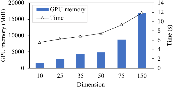
Figure 2: GPU memory cost and running time of each epoch w.r.t. different dimensions on DBP15K ZH-EN.

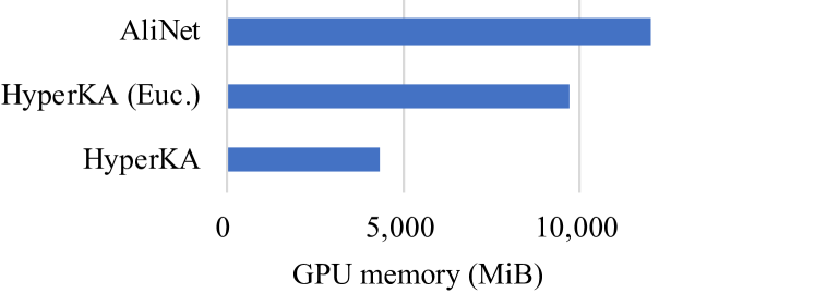
Figure 3: GPU memory cost of training HyperKA and its Euclidean counterpart HyperKA (Euc.) as well as AliNet Sun et al. (2020a) on DBP15K ZH-EN when they achieve similar performance. The dimension settings that they need are respectively (35, 35, 35), (200, 200, 200) and (500, 400, 300), and their H@1 scores are 0.532, 0.549 and 0.539, respectively.

We report in Figure 2 the GPU memory costs for training HyperKA in 64-bit precision settings w.r.t. various dimensions on ZH-EN, together with the average training time per epoch. A larger dimension leads to more GPU memory costs and training time, although it also leads to better performance as shown in Table 3. HyperKA can achieve satisfying performance with limited GPU memory costs.

5.1.4 Analysis on Expressiveness

To further understand the expressiveness of our hyperbolic KG embeddings, we compare a small dimension along with their GPU memory costs of HyperKA and its Euclidean counterpart HyperKA (Euc.) with AliNet, when those three achieve similar performance. HyperKA (Euc.) is implemented by replacing hyperbolic operations with their corresponding Euclidean operations. For example, the Möbius addition $\oplus$ is replaced with vector addition $+$. We select the dimension of HyperKA (Euc.) in $\{75,100,150,200,300,500\}$ and its best-performing model under the dimension of 200 can achieve similar performance to AliNet. By contrast, HyperKA only needs a dimension of 35 as shown in Table 3. Their GPU memory costs on ZH-EN are shown in Figure 3. We observe similar results on JA-EN and FR-EN. Specifically, HyperKA only costs about 45.09% memory of HyperKA (Euc.) and 29.97% of AliNet to achieve similar performance. This shows that hyperbolic embeddings can achieve satisfying expressiveness with a small dimension and efficient memory costs.

Datasets	Dimensions	H@1	H@10	MRR
ZH-EN	200, 200, 200	0.549	0.827	0.650
JA-EN	200, 200, 200	0.527	0.813	0.631
FR-EN	200, 200, 200	0.567	0.864	0.675
ZH-EN	300, 300, 300	0.581	0.857	0.683
JA-EN	300, 300, 300	0.563	0.844	0.666
FR-EN	300, 300, 300	0.605	0.896	0.711

Table 4: Entity alignment results of HyperKA (Euc.).

Methods	ZH-EN		JA-EN		FR-EN
	H@1	MRR	H@1	MRR	H@1	MRR
BootEA Sun et al. (2018)	0.629	0.703	0.622	0.701	0.653	0.731
NAEA Zhu et al. (2019)	0.650	0.720	0.641	0.718	0.673	0.752
TransEdge Sun et al. (2019)	0.735	0.801	0.719	0.795	0.710	0.796
HyperKA (semi)	0.743	0.805	0.727	0.793	0.741	0.813

Table 5: H@1 and MRR results of semi-supervised entity alignment on DBP15K. Their dimension is 75.

Methods	Dimensions		YAGO26K-906			DB111K-174
	Entity	Concept	H@1	H@3	MRR	H@1	H@3	MRR
TransE Bordes et al. (2013)	300	50	0.732	0.353	0.144	0.437	0.608	0.503
DistMult Yang et al. (2015)	300	50	0.361	0.553	0.411	0.498	0.680	0.551
HolE Nickel et al. (2016)	300	50	0.348	0.548	0.395	0.448	0.654	0.504
MTransE Chen et al. (2017)	300	50	0.609	0.776	0.689	0.599	0.813	0.672
JOIE Hao et al. (2019)	300	50	0.856	0.959	0.897	0.756	0.959	0.857
HyperKA	75	15	0.863	0.946	0.908	0.778	0.918	0.854
HyperKA	150	30	0.871	0.948	0.913	0.789	0.927	0.863

Table 6: Type inference results on YAGO26K-906 and DB111K-174.

We report in Table 4 the entity alignment results of HyperKA (Euc.) on DBP15K. We can find that HyperKA (Euc.) with a high dimension (e.g., 300) can also achieve similar performance with HyperKA at a low dimension of 75. This is because the Euclidean embeddings also have enough expressiveness to represent hierarchical structures if given a large dimension. However, hyperbolic embeddings only need a small dimension, bringing along the substantial advantage in saving memory.

5.1.5 Semi-supervised Entity Alignment

Semi-supervised entity alignment methods use self-training or co-training techniques to augment training data by iteratively finding new alignment labels Sun et al. (2018); Zhu et al. (2019); Sun et al. (2019). Following BootEA Sun et al. (2018), we use the self-training strategy to iteratively propose more aligned entity pairs to augment training data, denoted as $\mathcal{A}^{\prime}=\{(i,j)\in\mathcal{E}_{1}\times\mathcal{E}_{2}\,|\,\pi(i,j)<\epsilon\}$, where $\epsilon$ is a distance threshold. As these pairs inevitably contains errors Sun et al. (2018), we apply a small weight $\mu$ when using such proposed data for training, resulting in the following loss:

$$\mathcal{L}_{\text{semi}}=\mu\sum_{(i,j)\in\mathcal{A}^{\prime}}\pi(i,j).$$ (13)

Accordingly, the semi-supervised HyperKA variant minimizes the joint loss $\mathcal{L}+\mathcal{L}_{\text{semi}}$. The selected settings are $\epsilon=0.25$, $\mu=0.05$, and the training takes 800 epochs. Table 5 lists the H@1 and MRR results, where HyperKA shows drastic improvement over BootEA and NAEA. It also achieves noticeably better H@1 than the latest semi-supervised method TransEdge, especially on the FR-EN setting. The good performance of TransEdge comes with prohibitive memory overhead. Its parameter complexity is $O(2N_{e}n+N_{r}n)$ Sun et al. (2019), where $N_{e}$ and $N_{r}$ denote the numbers of entities and relations in KGs, respectively. $n$ is the dimension. By contrast, the complexity of our method is $O(N_{e}n+N_{r}n+Ln^{2})$ and we have $N_{e}\gg Ln$ in practice, where $L$ is the number of GNN layers. In this case, HyperKA outclasses TransEdge in both effectiveness and efficiency. Compared with our results in Table 2, we find that the self-training, being an optional and compatible technique, brings an improvement of more than 0.14 on H@1.

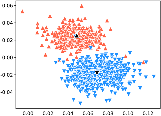
Figure 4: Visualization of the embeddings generated by HyperKA for two related concepts “Film” and “Album” along with their entities in DB111K-174. The black up triangle denotes “Film” and the surrounding red ones are its entities. The black down triangle denotes “Album” and the blue ones are its entities.

5.2 Type Inference

The main difference between type inference and entity alignment lies in that the knowledge to associate in the former scenario differs much in scales and specificity. This causes many related methods based on shared embedding spaces to fall short.

5.2.1 Experimental Setup

Datasets. The experiments for this task are conducted on datasets YAGO26K-906 and DB111K-174 Hao et al. (2019), which are extracted from YAGO and DBpedia, respectively. Each dataset has an entity-level KG and an ontological KG for concepts (types). Their statistics are reported in Appendix A. To compare with the previous work Hao et al. (2019), we use the original data splits, and report H@1, H@3 and MRR results. The hyper-parameter settings are listed in Appendix B.

Baselines. So far, only a few methods have been applied to the type inference task in KGs. We compare with the SOTA method JOIE Hao et al. (2019), and four other baseline methods TransE Bordes et al. (2013), DistMult Yang et al. (2015), HolE Nickel et al. (2016) and MTransE Chen et al. (2017) that are reported in the same paper. For JOIE, we choose its best-performing variant based on the translational encoder with cross-view transformation. A related method Jin et al. (2019) is not taken into comparison as it requires entity attributes that are unavailable in our problem setting.

5.2.2 Main Results

In this task, the embedding dimensions for entities and concepts are different, i.e., $n>m$, as an entity-level KG usually contains much more entities than concepts in a related ontological (or concept-level) KG. For HyperKA, we evaluate two dimension settings: $n=75,m=15$ and $n=150,m=30$. Both are much smaller than the dimensions of baseline methods. The results are reported in Table 6. We can observe that HyperKA (75, 15) outperforms JOIE in terms of H@1 on both datasets, especially on DBP111K-174, although HyperKA uses a much smaller dimension. For example, the H@1 score of HyperKA (75, 15) on DB111K-174 reaches 0.778, with a gain of 0.022 over JOIE in its best setting. HyperKA (150, 30) achieves the best performance over H@1 and MRR. We also try the dimension setting of (300, 50), but no longer observe further improvement. We believe this is because the dimension setting (150, 30) is enough for type inference as the concept-level KG is small. Meanwhile, once we apply the same small-dimension setting (75, 15) as HyperKA to baseline methods, the performance of those methods become much worse. For example, MTransE achieves no more than 0.357 in H@1 using this small dimension.

5.2.3 Case Study

For case study, we visualize the embeddings of two related concepts “Film” and “Album” in DBP111K-174 along with their associated entities in the PCA-projected space in Figure 4. Despite these two groups of entities are closely relevant, the embeddings learned by HyperKA are able to clearly distinguish between these two. We can see that the entities of the same type are embedded closely after transformation, while the two clusters are generally well differentiated by a clear margin (with only a few exceptions). This displays how the hyperbolic transformation is able to capture the multi-granular associations, while preserves the gap between the entities associated with different concepts.

6 Conclusion and Future Work

We propose a method to capture knowledge associations with a new hyperbolic GNN-based representation learning model. The proposed HyperKA method extends translational and GNN-based techniques to hyperbolic spaces, and captures associations by a hyperbolic transformation. Our method outperforms SOTA baselines using lower embedding dimensions on both entity alignment and type inference. For future work, we plan to incorporate hyperbolic RNNs Ganea et al. (2018) to encode auxiliary information for zero-shot entity and concept representations. Another meaningful direction is to use HyperKA to infer the associations between snapshots in temporally dynamic KGs Xu et al. (2020). We also seek to investigate the use of HyperKA for cross-domain representations of biological and medical knowledge Hao et al. (2020).

Acknowledgments. We thank the anonymous re- viewers for their insightful comments. This work is supported by the National Natural Science Foundation of China (Nos. 61872172 and 61772264), and the Collaborative Innovation Center of Novel Software Technology and Industrialization.

Appendix A Dataset Statistics

Table 7 lists the statistics of the entity alignment dataset DBP15K Sun et al. (2017), as well as two type inference datasets YAGO26K-906 and DB111K-174 Hao et al. (2019). For a fair comparison, we reuse the original splits of associations in these datasets for training and evaluation, i.e., 30% alignment in DBP15K as well as around 60% associations in YAGO26K-906 and DB111K-174 as training data. We can see that the two KGs of type inference datasets differs much more in terms of the scales of objects and triples than those in entity alignment datasets, which also bring along more challenges to knowledge association.

Datasets			#Objects	#Rel.	#Triples	#Assoc.
DBP15K	ZH-EN	ZH	66,469	2,830	153,929	15,000
		EN	98,125	2,317	237,674
	JA-EN	JA	65,744	2,043	164,373	15,000
		EN	95,680	2,096	233,319
	FR-EN	FR	66,858	1,379	192,191	15,000
		EN	105,889	2,209	278,590
YAGO26K-906		Ent.	26,078	34	390,738	9,962
		Ont.	906	30	8,962
DB111K-174		Ent.	111,762	305	863,643	99,748
		Ont.	174	20	763

Table 7: Statistics of the datasets used in this paper.

Appendix B Hyper-parameter Settings

In this section, we report the implementation details and hyper-parameter settings of HyperKA on the two knowledge association tasks. We select each hyper-parameter setting within a wide range of values as follows:

• Learning rate: $\{0.0001,0.0002,0.0005,0.001\}$

• Batch size: $\{2000,5000,10000,20000,50000\}$

• # GNN layers: $\{1,2,3,4,5\}$

• # Negative samples: $\{1,10,20,30,40,50,100\}$

• $\lambda_{1}$: $\{0.01,0.02,0.05,0.1,0.15,0.2,0.3,0.4\}$

• $\lambda_{2}$: $\{0.01,0.02,0.05,0.1,0.15,0.2,0.3,0.4\}$

Table 8 lists the selected hyper-parameter settings for the best-performing models (measured by H@1 scores) of HyperKA with 75 dimension for entity alignment on DBP15K, as well as (75, 15) dimensions for type inference on YAGO26K-906 and DB111K-174. We use truncated negative sampling and cross-domain similarity local scaling for the entity alignment task. The training takes 800 epochs on DBP15K, 60 epochs on YAGO26K-906 and 100 epochs on DB111K-174. The activation function used in our method is $\tanh$.

Parameters	DBP15K	YAGO26K-906	DB111K-174
Learning rate	0.0002	0.0005	0.0005
Batch size	20,000	2,000	20,000
# GNN layers	2	3	3
# Neg. samples	40	40	30
$\lambda_{1}$	0.1	0.2	0.2
$\lambda_{2}$	0.4	0.1	0.1

Table 8: Selected values for hyper-parameters.

References

- Aly et al. (2019) Rami Aly, Shantanu Acharya, Alexander Ossa, Arne Köhn, Chris Biemann, and Alexander Panchenko. 2019. Every child should have parents: A taxonomy refinement algorithm based on hyperbolic term embeddings. In Proceedings of the Annual Meeting of the Association for Computational Linguistics (ACL), pages 4811–4817.
- Balazevic et al. (2019) Ivana Balazevic, Carl Allen, and Timothy M. Hospedales. 2019. Multi-relational poincaré graph embeddings. In Proceedings of the Annual Conference on Neural Information Processing Systems (NeurIPS), pages 4465–4475.
- Bonnabel (2013) Silvere Bonnabel. 2013. Stochastic gradient descent on riemannian manifolds. IEEE Transactions on Automatic Control, 58(9):2217–2229.
- Bordes et al. (2013) Antoine Bordes, Nicolas Usunier, Alberto García-Durán, Jason Weston, and Oksana Yakhnenko. 2013. Translating embeddings for modeling multi-relational data. In Proceedings of the Annual Conference on Neural Information Processing Systems (NeurIPS), pages 2787–2795.
- Cannon et al. (1997) James W Cannon, William J Floyd, Richard Kenyon, and Walter R Parry. 1997. Hyperbolic geometry. Flavors of geometry, 31:59–115.
- Cao et al. (2019) Yixin Cao, Zhiyuan Liu, Chengjiang Li, Zhiyuan Liu, Juanzi Li, and Tat-Seng Chua. 2019. Multi-channel graph neural network for entity alignment. In Proceedings of the Annual Meeting of the Association for Computational Linguistics (ACL), pages 1452–1461.
- Chami et al. (2019) Ines Chami, Rex Ying, Christopher Ré, and Jure Leskovec. 2019. Hyperbolic graph convolutional neural networks. In Proceedings of the Annual Conference on Neural Information Processing Systems (NeurIPS), pages 4869–4880.
- Chen et al. (2019) Jiaao Chen, Jianshu Chen, and Zhou Yu. 2019. Incorporating structured commonsense knowledge in story completion. In Proceedings of the AAAI Conference on Artificial Intelligence (AAAI), pages 6244–6251.
- Chen and Quirk (2019) Muhao Chen and Chris Quirk. 2019. Embedding edge-attributed relational hierarchies. In Proceedings of the Annual International ACM SIGIR Conference on Research and Development in Information Retrieval (SIGIR), pages 873–876.
- Chen et al. (2018) Muhao Chen, Yingtao Tian, Kai-Wei Chang, Steven Skiena, and Carlo Zaniolo. 2018. Co-training embeddings of knowledge graphs and entity descriptions for cross-lingual entity alignment. In Proceedings of the International Joint Conference on Artificial Intelligence (IJCAI), pages 3998–4004.
- Chen et al. (2017) Muhao Chen, Yingtao Tian, Mohan Yang, and Carlo Zaniolo. 2017. Multilingual knowledge graph embeddings for cross-lingual knowledge alignment. In Proceedings of the International Joint Conference on Artificial Intelligence (IJCAI), pages 1511–1517.
- Dhingra et al. (2018) Bhuwan Dhingra, Christopher J. Shallue, Mohammad Norouzi, Andrew M. Dai, and George E. Dahl. 2018. Embedding text in hyperbolic spaces. In Proceedings of the Workshop on Graph-Based Methods for Natural Language Processing (TextGraphs@NAACL-HLT), pages 59–69.
- Dong et al. (2019) Tiansi Dong, Zhigang Wang, Juanzi Li, Christian Bauckhage, and Armin B. Cremers. 2019. Triple classification using regions and fine-grained entity typing. In Proceedings of the AAAI Conference on Artificial Intelligence (AAAI), pages 77–85.
- Ganea et al. (2018) Octavian-Eugen Ganea, Gary Bécigneul, and Thomas Hofmann. 2018. Hyperbolic neural networks. In Proceedings of the Annual Conference on Neural Information Processing Systems (NeurIPS), pages 5350–5360.
- Gesese et al. (2019) Genet Asefa Gesese, Russa Biswas, Mehwish Alam, and Harald Sack. 2019. A survey on knowledge graph embeddings with literals: Which model links better literal-ly? Semantic Web Journal.
- Guo et al. (2019) Lingbing Guo, Zequn Sun, and Wei Hu. 2019. Learning to exploit long-term relational dependencies in knowledge graphs. In Proceedings of the International Conference on Machine Learning (ICML), pages 2505–2514.
- Hao et al. (2019) Junheng Hao, Muhao Chen, Wenchao Yu, Yizhou Sun, and Wei Wang. 2019. Universal representation learning of knowledge bases by jointly embedding instances and ontological concepts. In Proceedings of the ACM SIGKDD International Conference on Knowledge Discovery and Data Mining (KDD), pages 1709–1719.
- Hao et al. (2020) Junheng Hao, Chelsea Ju, Muhao Chen, Yizhou Sun, Carlo Zaniolo, and Wei Wang. 2020. Bio-joie: Joint representation learning of biological knowledge bases. In Proceedings of the 11st ACM Conference on Bioinformatics, Computational Biology and Biomedicine.
- Hixon et al. (2015) Ben Hixon, Peter Clark, and Hannaneh Hajishirzi. 2015. Learning knowledge graphs for question answering through conversational dialog. In Proceedings of the North American Chapter of the Association for Computational Linguistics (NAACL), pages 851–861.
- Hu et al. (2015) Zhiting Hu, Poyao Huang, Yuntian Deng, Yingkai Gao, and Eric P. Xing. 2015. Entity hierarchy embedding. In Proceedings of the Annual Meeting of the Association for Computational Linguistics (ACL), pages 1292–1300.
- Jin et al. (2019) Hailong Jin, Lei Hou, Juanzi Li, and Tiansi Dong. 2019. Fine-grained entity typing via hierarchical multi graph convolutional networks. In Proceedings of the Conference on Empirical Methods in Natural Language Processing and the International Joint Conference on Natural Language Processing (EMNLP-IJCNLP), pages 4968–4977.
- Kingma and Ba (2015) Diederik P. Kingma and Jimmy Ba. 2015. Adam: A method for stochastic optimization. In Proceedings of the International Conference on Learning Representations (ICLR).
- Kipf and Welling (2017) Thomas N. Kipf and Max Welling. 2017. Semi-supervised classification with graph convolutional networks. In Proceedings of the International Conference on Learning Representations (ICLR).
- Kolyvakis et al. (2020) Prodromos Kolyvakis, Alexandros Kalousis, and Dimitris Kiritsis. 2020. Hyperbolic knowledge graph embeddings for knowledge base completion. In Proceedings of the Extended Semantic Web Conference (ESWC), pages 199–214.
- Krioukov et al. (2010) Dmitri V. Krioukov, Fragkiskos Papadopoulos, Maksim Kitsak, Amin Vahdat, and Marián Boguñá. 2010. Hyperbolic geometry of complex networks. CoRR, abs/1006.5169.
- Lacoste-Julien et al. (2013) Simon Lacoste-Julien, Konstantina Palla, Alex Davies, Gjergji Kasneci, Thore Graepel, and Zoubin Ghahramani. 2013. SIGMa: simple greedy matching for aligning large knowledge bases. In Proceedings of the ACM SIGKDD International Conference on Knowledge Discovery and Data Mining (KDD), pages 572–580.
- Le et al. (2019) Matt Le, Stephen Roller, Laetitia Papaxanthos, Douwe Kiela, and Maximilian Nickel. 2019. Inferring concept hierarchies from text corpora via hyperbolic embeddings. In Proceedings of the Annual Meeting of the Association for Computational Linguistics (ACL), pages 3231–3241.
- Lehmann et al. (2015) Jens Lehmann, Robert Isele, Max Jakob, Anja Jentzsch, Dimitris Kontokostas, Pablo N. Mendes, Sebastian Hellmann, Mohamed Morsey, Patrick van Kleef, Sören Auer, and Christian Bizer. 2015. Dbpedia - A large-scale, multilingual knowledge base extracted from wikipedia. Semantic Web, 6(2):167–195.
- Li et al. (2019) Chengjiang Li, Yixin Cao, Lei Hou, Jiaxin Shi, Juanzi Li, and Tat-Seng Chua. 2019. Semi-supervised entity alignment via joint knowledge embedding model and cross-graph model. In Proceedings of the Conference on Empirical Methods in Natural Language Processing and the International Joint Conference on Natural Language Processing (EMNLP-IJCNLP), pages 2723–2732.
- Lin et al. (2019) Xixun Lin, Hong Yang, Jia Wu, Chuan Zhou, and Bin Wang. 2019. Guiding cross-lingual entity alignment via adversarial knowledge embedding. In Proceedings of the IEEE International Conference on Data Mining (ICDM), pages 429–438.
- Liu et al. (2019) Qi Liu, Maximilian Nickel, and Douwe Kiela. 2019. Hyperbolic graph neural networks. In Proceedings of the Annual Conference on Neural Information Processing Systems (NeurIPS), pages 8228–8239.
- Lv et al. (2018) Xin Lv, Lei Hou, Juanzi Li, and Zhiyuan Liu. 2018. Differentiating concepts and instances for knowledge graph embedding. In Proceedings of the Conference on Empirical Methods in Natural Language Processing (EMNLP), pages 1971–1979.
- Mao et al. (2020) Xin Mao, Wenting Wang, Huimin Xu, Man Lan, and Yuanbin Wu. 2020. MRAEA: an efficient and robust entity alignment approach for cross-lingual knowledge graph. In Proceedings of the ACM International Conference on Web Search and Data Mining (WSDM), pages 420–428.
- Mitchell et al. (2018) Tom M. Mitchell, William W. Cohen, Estevam R. Hruschka Jr., Partha P. Talukdar, Bo Yang, Justin Betteridge, Andrew Carlson, Bhavana Dalvi Mishra, Matt Gardner, Bryan Kisiel, et al. 2018. Never-ending learning. Communications of the ACM, 61(5):103–115.
- Moon et al. (2019) Seungwhan Moon, Pararth Shah, Anuj Kumar, and Rajen Subba. 2019. OpenDialKG: Explainable conversational reasoning with attention-based walks over knowledge graphs. In Proceedings of the Annual Meeting of the Association for Computational Linguistics (ACL), pages 845–854.
- Nickel et al. (2014) Maximilian Nickel, Xueyan Jiang, and Volker Tresp. 2014. Reducing the rank in relational factorization models by including observable patterns. In Proceedings of the Annual Conference on Neural Information Processing Systems (NeurIPS), pages 1179–1187.
- Nickel and Kiela (2017) Maximilian Nickel and Douwe Kiela. 2017. Poincaré embeddings for learning hierarchical representations. In Proceedings of the Annual Conference on Neural Information Processing Systems (NeurIPS), pages 6338–6347.
- Nickel et al. (2016) Maximilian Nickel, Lorenzo Rosasco, and Tomaso A. Poggio. 2016. Holographic embeddings of knowledge graphs. In Proceedings of the AAAI Conference on Artificial Intelligence (AAAI), pages 1955–1961.
- Nielsen and Nock (2014) Frank Nielsen and Richard Nock. 2014. Visualizing hyperbolic voronoi diagrams. In Proceedings of the International Symposium on Computational Geometry (SoCG), page 90.
- Nikolov et al. (2009) Andriy Nikolov, Victoria S. Uren, Enrico Motta, and Anne N. De Roeck. 2009. Overcoming schema heterogeneity between linked semantic repositories to improve coreference resolution. In Proceedings of the Asian Semantic Web Conference (ASWC), pages 332–346.
- Paulheim and Bizer (2013) Heiko Paulheim and Christian Bizer. 2013. Type inference on noisy RDF data. In Proceedings of the International Semantic Web Conference (ISWC), pages 510–525.
- Pei et al. (2019a) Shichao Pei, Lu Yu, Robert Hoehndorf, and Xiangliang Zhang. 2019a. Semi-supervised entity alignment via knowledge graph embedding with awareness of degree difference. In Proceedings of The Web Conference (WWW), pages 3130–3136.
- Pei et al. (2019b) Shichao Pei, Lu Yu, and Xiangliang Zhang. 2019b. Improving cross-lingual entity alignment via optimal transport. In Proceedings of the International Joint Conference on Artificial Intelligence (IJCAI), pages 3231–3237.
- Reynolds (1993) William F. Reynolds. 1993. Hyperbolic geometry on a hyperboloid. The American Mathematical Monthly, 100(5):442–455.
- Sala et al. (2018) Frederic Sala, Christopher De Sa, Albert Gu, and Christopher Ré. 2018. Representation tradeoffs for hyperbolic embeddings. In Proceedings of the International Conference on Machine Learning (ICML), pages 4457–4466.
- Schlichtkrull et al. (2018) Michael Sejr Schlichtkrull, Thomas N. Kipf, Peter Bloem, Rianne van den Berg, Ivan Titov, and Max Welling. 2018. Modeling relational data with graph convolutional networks. In Proceedings of the Extended Semantic Web Conference (ESWC), pages 593–607.
- Shi and Xiao (2019) Xiaofei Shi and Yanghua Xiao. 2019. Modeling multi-mapping relations for precise cross-lingual entity alignment. In Proceedings of the Conference on Empirical Methods in Natural Language Processing and the International Joint Conference on Natural Language Processing (EMNLP-IJCNLP), pages 813–822.
- Speer et al. (2017) Robyn Speer, Joshua Chin, and Catherine Havasi. 2017. Conceptnet 5.5: An open multilingual graph of general knowledge. In Proceedings of the AAAI Conference on Artificial Intelligence (AAAI), pages 4444–4451.
- Suchanek et al. (2011) Fabian M. Suchanek, Serge Abiteboul, and Pierre Senellart. 2011. PARIS: probabilistic alignment of relations, instances, and schema. Proceedings of the VLDB Endowment, 5(3):157–168.
- Sun et al. (2017) Zequn Sun, Wei Hu, and Chengkai Li. 2017. Cross-lingual entity alignment via joint attribute-preserving embedding. In Proceedings of the International Semantic Web Conference (ISWC), pages 628–644.
- Sun et al. (2018) Zequn Sun, Wei Hu, Qingheng Zhang, and Yuzhong Qu. 2018. Bootstrapping entity alignment with knowledge graph embedding. In Proceedings of the International Joint Conference on Artificial Intelligence (IJCAI), pages 4396–4402.
- Sun et al. (2019) Zequn Sun, Jiacheng Huang, Wei Hu, Muhao Chen, Lingbing Guo, and Yuzhong Qu. 2019. Transedge: Translating relation-contextualized embeddings for knowledge graphs. In Proceedings of the International Semantic Web Conference (ISWC), pages 612–629.
- Sun et al. (2020a) Zequn Sun, Chengming Wang, Wei Hu, Muhao Chen, Jian Dai, Wei Zhang, and Yuzhong Qu. 2020a. Knowledge graph alignment network with gated multi-hop neighborhood aggregation. In Proceedings of the AAAI Conference on Artificial Intelligence (AAAI), pages 222–229.
- Sun et al. (2020b) Zequn Sun, Qingheng Zhang, Wei Hu, Chengming Wang, Muhao Chen, Farahnaz Akrami, and Chengkai Li. 2020b. A benchmarking study of embedding-based entity alignment for knowledge graphs. Proceedings of the VLDB Endowment, 13(11):2326–2340.
- Tifrea et al. (2019) Alexandru Tifrea, Gary Bécigneul, and Octavian-Eugen Ganea. 2019. Poincare glove: Hyperbolic word embeddings. In Proceedings of the International Conference on Learning Representations (ICLR).
- Trisedya et al. (2019) Bayu Distiawan Trisedya, Jianzhong Qi, and Rui Zhang. 2019. Entity alignment between knowledge graphs using attribute embeddings. In Proceedings of the AAAI Conference on Artificial Intelligence (AAAI), pages 297–304.
- Trivedi et al. (2018) Rakshit Trivedi, Bunyamin Sisman, Xin Luna Dong, Christos Faloutsos, Jun Ma, and Hongyuan Zha. 2018. LinkNBed: Multi-graph representation learning with entity linkage. In Proceedings of the Annual Meeting of the Association for Computational Linguistics (ACL), pages 252–262.
- Vashishth et al. (2020) Shikhar Vashishth, Soumya Sanyal, Vikram Nitin, and Partha Talukdar. 2020. Composition-based multi-relational graph convolutional networks. In Proceedings of the International Conference on Learning Representations (ICLR).
- Vinh et al. (2018) Tran Dang Quang Vinh, Yi Tay, Shuai Zhang, Gao Cong, and Xiao-Li Li. 2018. Hyperbolic recommender systems. CoRR, abs/1809.01703.
- Wang et al. (2018) Zhichun Wang, Qingsong Lv, Xiaohan Lan, and Yu Zhang. 2018. Cross-lingual knowledge graph alignment via graph convolutional networks. In Proceedings of the Conference on Empirical Methods in Natural Language Processing (EMNLP), pages 349–357.
- Wu et al. (2019a) Yuting Wu, Xiao Liu, Yansong Feng, Zheng Wang, Rui Yan, and Dongyan Zhao. 2019a. Relation-aware entity alignment for heterogeneous knowledge graphs. In Proceedings of the International Joint Conference on Artificial Intelligence (IJCAI), pages 5278–5284.
- Wu et al. (2019b) Yuting Wu, Xiao Liu, Yansong Feng, Zheng Wang, and Dongyan Zhao. 2019b. Jointly learning entity and relation representations for entity alignment. In Proceedings of the Conference on Empirical Methods in Natural Language Processing and the International Joint Conference on Natural Language Processing (EMNLP-IJCNLP), pages 240–249.
- Xu et al. (2020) Da Xu, Chuanwei Ruan, Evren Körpeoglu, Sushant Kumar, and Kannan Achan. 2020. Inductive representation learning on temporal graphs. In Proceedings of the International Conference on Learning Representations (ICLR).
- Yang et al. (2015) Bishan Yang, Wen-tau Yih, Xiaodong He, Jianfeng Gao, and Li Deng. 2015. Embedding entities and relations for learning and inference in knowledge bases. In Proceedings of the International Conference on Learning Representations (ICLR).
- Yang et al. (2019) Hsiu-Wei Yang, Yanyan Zou, Peng Shi, Wei Lu, Jimmy Lin, and Xu Sun. 2019. Aligning cross-lingual entities with multi-aspect information. In Proceedings of the Conference on Empirical Methods in Natural Language Processing and the International Joint Conference on Natural Language Processing (EMNLP-IJCNLP), pages 4430–4440.
- Ye et al. (2019) Rui Ye, Xin Li, Yujie Fang, Hongyu Zang, and Mingzhong Wang. 2019. A vectorized relational graph convolutional network for multi-relational network alignment. In Proceedings of the International Joint Conference on Artificial Intelligence (IJCAI), pages 4135–4141.
- Zhang et al. (2019) Qingheng Zhang, Zequn Sun, Wei Hu, Muhao Chen, Lingbing Guo, and Yuzhong Qu. 2019. Multi-view knowledge graph embedding for entity alignment. In Proceedings of the International Joint Conference on Artificial Intelligence (IJCAI), pages 5429–5435.
- Zhu et al. (2017) Hao Zhu, Ruobing Xie, Zhiyuan Liu, and Maosong Sun. 2017. Iterative entity alignment via joint knowledge embeddings. In Proceedings of the International Joint Conference on Artificial Intelligence (IJCAI), pages 4258–4264.
- Zhu et al. (2019) Qiannan Zhu, Xiaofei Zhou, Jia Wu, Jianlong Tan, and Li Guo. 2019. Neighborhood-aware attentional representation for multilingual knowledge graphs. In Proceedings of the International Joint Conference on Artificial Intelligence (IJCAI), pages 1943–1949.