Approaching the Full Configuration Interaction Ground State from an Arbitrary Wavefunction with Gradient Descent and Quasi-Newton Algorithms

Abstract

We consider gradient descent and quasi-Newton algorithms to optimize the full configuration interaction (FCI) ground state wavefunction starting from an arbitrary reference state $|0\rangle$. We show that the energies obtained along the optimization path can be evaluated in terms of expectation values of $|0\rangle$, thus avoiding explicit storage of intermediate wavefunctions. This allows us to find the energies after the first few steps of the FCI algorithm for systems much larger than what standard, deterministic FCI codes can handle at present. We show an application of the algorithm with reference wavefunctions constructed as linear combinations of non-orthogonal determinants.

I Introduction

In principle, all the chemical properties of molecular systems can be determined from knowledge of the eigenstates of the Hamiltonian operator. The full-configuration interaction (FCI) wavefunction constitutes a prominent paradigm of quantum chemistry Szabo and Ostlund (1989): it provides the exact solution of the Schrödinger equation on a basis of suitably selected $N$-electron wavefunctions. While finding the FCI ground state wavefunction is algorithmically easy, the number of degrees of freedom in it increases exponentially with system size. Therefore, one of the central goals of the quantum chemistry community is to develop approximations that can yield properties of similar quality as that from the FCI ground state while reducing significantly the computational cost entailed.

The optimization of the FCI ground state wavefunction is usually cast as an eigenvalue problem. Given a matrix representation of the Hamiltonian operator $H$ and a vector representation of a starting reference wavefunction $|0\rangle$, potent algorithms (with that from Davidson Davidson (1975) being a prominent example) have been developed to optimize the FCI ground state wavefunction $|\Psi_{\mathrm{FCI}}\rangle$ while minimizing the number of matrix-vector operations and the number of intermediate wavefunctions. Nevertheless, the dimension of the FCI problem renders this approach possible only for relatively small systems.

In this work, we obtain the FCI ground state from an unconstrained optimization of the wavefunction amplitudes in the orthogonal complement of some reference state $|0\rangle$. We carry the unconstrained optimization with gradient descent and quasi-Newton algorithms. In this way, the reference wavefunction is improved systematically with increasing number of steps. The central result obtained in this work is that the energies obtained along the optimization path can be fully expressed in terms of matrix elements of the reference $|0\rangle$. Explicitly casting the energy after some finite number of steps as a functional of the reference wavefunction allows us to consider systems for which the dimension of the Hilbert space is much larger than the disk or memory available in current computational facilities.

There is another important reason to avoid the explicit vector representation of the FCI wavefunction, which actually constitutes the motivation for this manuscript. Namely, it allows us to consider classes of wavefunctions for which a vector representation in some convenient orthonormal $N$-electron basis is not available, and the computational cost of evaluating it would be proportional to the dimension of the Hilbert space. A specific example that we shall consider are reference states written as linear combination of a few determinants that are, in general, non-orthogonal (i.e., $\langle\Phi_{1}|\Phi_{2}\rangle\neq 0$):

$$|0\rangle=\sum_{q}f_{q}|\Phi_{q}\rangle.$$

In that case the orthogonal complement is not known a priori and the vector representation in a basis of, e.g., orthonormal Slater determinants can only be determined at great computational expense. This class of wavefunctions occur in non-orthogonal configuration interaction (NOCI) Sundstrom and Head-Gordon (2014) as well as in symmetry-projected Hartree–Fock methods Jiménez-Hoyos et al. (2012).

The rest of this manuscript is organized as follows. In Sec. II we describe how we parametrize the FCI ground state wavefunction and describe the gradient descent and quasi-Newton optimization algorithms considered. In Sec. III we discuss the application of the method in an H₄ ring and in the determination of spectroscopic constants of the N₂, O₂, and F₂ molecules. Finally, in Sec. IV we provide some closing remarks.

II Theory

We parametrize the FCI ground state $|\Psi_{\mathrm{FCI}}\rangle$ using an exponential, non-Hermitian ansatz of the form

$$|\Psi\rangle =\,\exp(\hat{Z})|0\rangle,$$ (1)

$$\hat{Z} =\,\sum_{x}Z_{x}|x\rangle\langle 0|,$$ (2)

where $|0\rangle$ is the reference wavefunction and $|x\rangle$ labels an orthonormal state in the orthogonal complement of $|0\rangle$. The FCI ground state can be reached after an unconstrained optimization in the parameters $Z$. (We note that the same parametrization was used in Ref. Wang et al., 2019, also casting FCI as an unconstrained minimization problem.) An important ingredient of this work is that an explicit construction of the states $\{|x\rangle\}$ is not necessary. We assume in what follows that $\langle 0|\Psi_{\mathrm{FCI}}\rangle\neq 0$.

Given $Z$ (as a vector of amplitudes), the energy of $|\Psi\rangle$ can be evaluated as

$$E[Z] \equiv\,\frac{\langle\Psi|H|\Psi\rangle}{\langle\Psi|\Psi\rangle}=\frac{\langle 0|\exp(\hat{Z}^{\dagger})H\exp(\hat{Z})|0\rangle}{\langle 0|\exp(\hat{Z}^{\dagger})\exp(\hat{Z})|0\rangle}$$

$$=\,\frac{H_{0}^{0}+H_{0}^{x}Z_{x}+Z^{x}H_{x}^{0}+Z^{x}H_{x}^{y}Z_{y}}{1+Z^{x}Z_{x}},$$ (3)

where $H_{\alpha}^{\beta}=\langle\alpha|H|\beta\rangle$, Einstein summation is implied and the indices $x,y$ run only over the orthogonal complement of $|0\rangle$. Here, we have used the fact that $\hat{Z^{2}}|0\rangle=0$. We have also assumed a real wavefunction $|0\rangle$ and real coefficients $Z$, as we do throughout this work.

The energy gradient with respect to the amplitudes in $Z$, evaluated at $Z=Y$ is given by

$$g_{x}\equiv\left.\frac{\partial E[Z]}{\partial Z^{x}}\right|_{Z=Y}=\frac{2H_{x}^{0}+2H_{x}^{y}Y_{y}-2E[Y]Y_{x}}{1+Y^{y}Y_{y}}.$$ (4)

Along the optimization paths described in the next subsections a line search is needed to minimize the energy of $E[Y+sX]$, with $Y$ being the vector of current amplitudes and $X$ the search direction, with respect to the step size $s$. Explicitly, $E[Y+sX]$ becomes

$$E[Y+sX]=\frac{E[Y](1+Y^{x}Y_{x})+s(H_{0}^{x}+Y^{y}H_{y}^{x})X_{x}+sX^{x}(H_{x}^{0}+H_{x}^{y}Y_{y})+s^{2}X^{x}H_{x}^{y}X_{y}}{(1+Y^{x}Y_{x})+sY^{x}X_{x}+sX^{x}Y_{x}+s^{2}X^{x}X_{x}}.$$ (5)

This is a rational equation in $s$ of the form

$$\frac{c+bs+as^{2}}{f+es+ds^{2}}.$$

Let $s_{\ast}$ be the value of $s$ that extremizes $E[Y+sX]$; this takes the form

$$s_{\ast}=\frac{(cd-af)\pm\sqrt{(cd-af)^{2}-(ae-bd)(bf-ce)}}{(ae-bd)}.$$

For convenience, we shall introduce the quantities $f_{1}=H_{0}^{0}$, $f_{2}=H_{0}^{y}H_{y}^{0}$, $f_{3}=H_{0}^{y}H_{y}^{z}H_{z}^{0}$, etc. Note that all those matrix elements can be evaluated in terms of expectation values from the reference wavefunction $|0\rangle$. For instance,

$$f_{2} =\,\langle 0|H^{2}|0\rangle-f_{1}\langle 0|H|0\rangle,$$ (6)

$$f_{3} =\,\langle 0|H^{3}|0\rangle-f_{1}\langle 0|H^{2}|0\rangle-f_{2}\langle 0|H|0\rangle.$$ (7)

II.1 Gradient Descent

We begin at $Z_{0}=0$ with $|\Psi_{0}\rangle=|0\rangle$. The gradient at $Z_{0}$ is

$$(g_{0})_{x} =\,\alpha_{0}H_{x}^{0},$$ (8)

with $\alpha_{0}=2$.

In a standard gradient descent implementation a line search would be performed along $-g_{0}$. It is common practice to accept a step size that satisfies Wolfe Wolfe (1969, 1971) conditions to avoid the potentially expensive full line search. In our case, we aim to perform a full line search, as we may only be able to afford a few steps. The optimal step size $\sigma_{\ast}$ can be easily found given the rational form of $E[Z]$ discussed above. Therefore, $Z_{1}=-\sigma_{\ast}g_{0}$ and $|\Psi_{1}\rangle$ becomes

$$|\Psi_{1}\rangle=e^{-\sigma_{\ast}g_{0}}|0\rangle.$$ (9)

An explicit expression for $E_{1}$ is given by

$$E_{1}\equiv\frac{\langle\Psi_{1}|H|\Psi_{1}\rangle}{\langle\Psi_{1}|\Psi_{1}\rangle}=\frac{f_{1}-2\sigma_{\ast}\alpha_{0}f_{2}+\sigma_{\ast}^{2}\alpha_{0}^{2}f_{3}}{1+\sigma_{\ast}^{2}\alpha_{0}^{2}f_{2}},$$ (10)

with

$$\sigma_{\ast}=\frac{(4f_{3}-4f_{1}f_{2})\pm\sqrt{64f_{2}^{3}+(4f_{3}-4f_{1}f_{2})^{2}}}{-16f_{2}^{2}}.$$ (11)

Note that $E_{1}$ is a functional of $|0\rangle$ which can be determined after evaluation of $f_{1}$, $f_{2}$, and $f_{3}$. (This is an interesting functional in itself. One may consider optimizing $E_{1}$ with respect to the reference wavefunction parameters $|0\rangle$, which we have done for one of the examples considered.)

We now proceed to take another step. The gradient at $Z_{1}=-\sigma_{\ast}g_{0}$ is given by

$$(g_{1})_{x}=\alpha_{1}H_{x}^{0}+\beta_{1}H_{x}^{y}H_{y}^{0}$$ (12)

with

$$\alpha_{1} =\,\frac{2(1+\sigma_{\ast}\alpha_{0}E_{1})}{1+\sigma_{\ast}^{2}\alpha_{0}^{2}f_{2}},$$ (13)

$$\beta_{1} =\,\frac{-2\sigma_{\ast}\alpha_{0}}{1+\sigma_{\ast}^{2}\alpha_{0}^{2}f_{2}}.$$ (14)

After looking for the optimal step size $\tau_{\ast}$ (i.e., minimizing $E[-\sigma_{\ast}g_{0}-\tau g_{1}]$ with respect to $\tau$), $|\Psi_{2}\rangle$ becomes

$$|\Psi_{2}\rangle=e^{-\sigma_{\ast}g_{0}-\tau_{\ast}g_{1}}|0\rangle.$$ (15)

An explicit expression for $E_{2}$ is given below

$$E_{2}\equiv\frac{\langle\Psi_{2}|H|\Psi_{2}\rangle}{\langle\Psi_{2}|\Psi_{2}\rangle}=\,\frac{E_{1}(1+\sigma_{\ast}^{2}\alpha_{0}^{2}f_{2})-2\tau_{\ast}(\alpha_{1}f_{2}+\beta_{1}f_{3})+2\sigma_{\ast}\tau_{\ast}\alpha_{0}(\alpha_{1}f_{3}+\beta_{1}f_{4})+\tau_{\ast}^{2}(\alpha_{1}^{2}f_{3}+2\alpha_{1}\beta_{1}f_{4}+\beta_{1}^{2}f_{5})}{(1+\sigma_{\ast}^{2}\alpha_{0}^{2}f_{2})+2\sigma_{\ast}\tau_{\ast}\alpha_{0}(\alpha_{1}f_{2}+\beta_{1}f_{3})+\tau_{\ast}^{2}(\alpha_{1}^{2}f_{2}+2\alpha_{1}\beta_{1}f_{3}+\beta_{1}^{2}f_{4})}.$$ (16)

A closed-form expression for $\tau_{\ast}$ can be deduced from the rational form of $E_{2}$ as a function of $\tau$, as described before. $E_{2}$ is also a functional of $|0\rangle$ that can be assembled after evaluation of $f_{1}$, …, $f_{5}$.

A third step would require the evaluation of $g_{2}$. Given the form of the gradient (Eq. 4), it can be shown that $g_{2}$ takes the form

$$(g_{2})_{x}=\alpha_{2}H_{x}^{0}+\beta_{2}H_{x}^{y}H_{y}^{0}+\gamma_{2}H_{x}^{y}H_{y}^{z}H_{z}^{0}.$$ (17)

Therefore, $E_{3}$ would be also a functional of $|0\rangle$ that can be determined after evaluation of $f_{1}$, …, $f_{7}$. Subsequent steps require the evaluation of higher order $f_{k}$ values.

At this point we note that the gradient descent approach described above can, in principle, be used to converge to the true eigenfunction of the Hamiltonian $\mathcal{H}$ as opposed to its representation in some finite $N$-electron basis $H$. It would involve replacing the expectation values $\langle 0|H^{k}|0\rangle$ with $\langle 0|\mathcal{H}^{k}|0\rangle$, with everything else holding. This, however, requires further work given that individual integrals appearing in $\mathcal{H}^{2}$ (and higher powers) diverge when evaluated with atomic Gaussian basis functions (see, e.g., Ref. Nakatsuji, 2012).

As a second remark, we note that the evaluation of other expectation values can be done in the same way as the energy. For instance, the expectation value of $W$, after the first gradient descent step, is given by

$$X_{1}\equiv\frac{\langle\Psi_{1}|W|\Psi_{1}\rangle}{\langle\Psi_{1}|\Psi_{1}\rangle}=\frac{f^{w}_{1}-2\sigma_{\ast}\alpha_{0}f^{w}_{2}+\sigma_{\ast}^{2}\alpha_{0}^{2}f^{w}_{3}}{1+\sigma_{\ast}^{2}\alpha_{0}^{2}f_{2}},$$ (18)

with $f^{w}_{1}=W_{0}^{0}$, $f^{w}_{2}=\frac{1}{2}(W_{0}^{y}H_{y}^{0}+H_{0}^{y}W_{y}^{0})$, $f^{w}_{3}=H_{0}^{y}W_{y}^{z}H_{z}^{0}$. This is also a functional of $|0\rangle$ since

$$f^{w}_{2} =\,\textstyle\frac{1}{2}\langle 0|WH+HW|0\rangle-f_{1}\langle 0|W|0\rangle,$$ (19)

$$f^{w}_{3} =\,\langle 0|HWH|0\rangle-\textstyle\frac{1}{2}f_{1}\langle 0|WH+HW|0\rangle$$

$$-\,f^{w}_{2}\langle 0|H|0\rangle.$$ (20)

II.2 Quasi-Newton

Because the convergence of the gradient descent algorithm is slow, we now consider a quasi-Newton optimization. In a quasi-Newton approach Nocedal and Wright (2006) it is customary to start from an initial inverse Hessian $B_{0}$, which need only be an approximation to the true Hessian. At each step along the optimization, the search direction $p_{k}$ is determined from $B_{k}p_{k}=-g_{k}$, rather than setting $p_{k}=-g_{k}$ as in the gradient descent approach. In this work we choose to set $B_{0}=I$ to keep things as simple as possible: under such conditions, a quasi-Newton algorithm can still be fully defined in terms of $|0\rangle$. Naturally, if a better $B_{0}$ is used the number of iterations required to reach convergence is expected to decrease.

Just as in the gradient descent approach, after defining a search direction $p_{k}$ a line search is performed along it. Commonly, a step size that satisfies Wolfe conditions is accepted. We choose, however, to carry a full line search as in the gradient descent algorithm.

Because $B_{0}=I$, it follows that the first step coincides with that from the gradient descent approach, and $E_{1}$ remains unchanged. The gradient $g_{1}$ is also the same as in gradient descent (see Eq. 12). The direction $p_{1}$ is determined from $p_{1}=-B_{1}g_{1}$, with $B_{1}$ constructed using a quasi-Newton update formula.

We show in appendix A that $p_{1}$, determined from a Broyden-Fletcher-Goldfarb-Shanno (BFGS) Broyden (1970); Fletcher (1970); Goldfarb (1970); Shanno (1970) update formula, takes the form

$$(p_{1})_{x}=\alpha^{\prime}_{1}H_{x}^{0}+\beta^{\prime}_{1}H_{x}^{y}H_{y}^{0},$$ (21)

with $\alpha^{\prime}_{1}$ and $\beta^{\prime}_{1}$ being some constants that are numerically different than $\alpha_{1}$ and $\beta_{1}$. Given that $p_{1}$ takes the same functional form as $g_{1}$, we conclude that $E_{2}$ determined from the BFGS approach is also a functional of $f_{1}$, …, $f_{5}$. Namely, $E_{2}$ would take the same form as Eq. 16, with $\alpha_{1}\to\alpha^{\prime}_{1}$ and $\beta_{1}\to\beta^{\prime}_{1}$. Further quasi-Newton steps can also be cast as functionals of $|0\rangle$, in the same way as in the gradient descent algorithm.

III Results and Discussion

We proceed to discuss the application of the optimization algorithms described above in a H₄ ring and in the N₂, O₂, and F₂ diatomics.

III.1 H₄ ring

We consider a system of 4 H atoms placed along a ring of radius $r=3.3$ bohr Qiu et al. (2017), with the arrangement depicted in Fig. 1. For $\theta\approx 24$ deg, the system consists of two weakly interacting H₂ molecules near their equilibrium geometry. Conversely, for $\theta=90$ deg the 4 H atoms form a square and the system has a strong multireference character. In scanning $\theta$ in the range between 20 deg and 90 deg the system evolves from a weak to a strong correlation regime. Our calculations in this system were performed by explicitly constructing the vector representation of the considered wavefunctions; this allows us to study the convergence behavior of the gradient descent and quasi-Newton algorithms.

Figure 1: The H₄ system described in Ref. Qiu et al., 2017 consists of four H atoms placed along a ring of radius $r=3.3$ bohr, controlled by an angle $\theta$. At $\theta\approx 24$ deg the system corresponds to two weakly interacting H₂ units near their equilibrium geometry.

We show in Fig. 2 (left) the energy of the H₄ system as a function of $\theta$, evaluated with the 6-31G basis set. In particular, we show restricted and unrestricted Hartree–Fock (RHF and UHF), spin-projected UHF (SUHF), and FCI ground state energies. In addition, we show the energy after the first and second gradient descent (gd) steps as well as the energy after the second quasi-Newton step starting from the RHF wavefunction. On the right we show the errors with respect to the FCI ground state calculated with each method, where we now show also the corrections starting from UHF and SUHF. The unusual profile displayed by the UHF curves is associated with the collapse back to the RHF wavefunction at $\theta\approx 40$ deg.

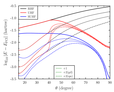
Figure 2: (Left) Energy (in hartree) of the H₄ system of Fig. 1, as a function of $\theta$, computed with various methods and the 6-31G basis set. We show the energies after 1 and 2 gradient descent (gd) steps, as well as the energy after 2 quasi-Newton (qn) steps. (Right) Error in the energy, with respect to the FCI ground state, after 1 and 2 gd or qn steps starting from RHF, UHF, and SUHF wavefunctions.

The improvement upon the RHF energy obtained with the first gd step is quite significant: the error is reduced by nearly a third at $\theta=90$ deg and by an order of magnitude in the equilibrium region. The second step (either gd or qn) reduces the energy even further, with the qn step being considerably better than the gd step. In the case of UHF and SUHF, the improvement after the first and second steps is very modest near $\theta=90$ deg, although the energy lowering near the equilibrium region is still substantial. Around $\theta\approx 50$ deg, the first step correction to RHF leads to a lower energy than the first step correction to UHF even when the reference wavefunction itself is lower in energy. As more steps are taken, the expectation is that the qn algorithm will outperform the gd algorithm as the former converges linearly while the latter should approach quadratic convergence Nocedal and Wright (2006).

We show in Fig. 3 the convergence profile of the gd and qn algorithms on top of the RHF, UHF, and SUHF wavefunctions at $\theta=24$ deg (top) and $\theta=90$ deg (bottom). At $\theta=24$ deg, convergence is relatively fast: with gd, 10 steps are sufficient to converge the energy to $10^{-5}$ hartree, while 5 steps are enough with the qn algorithm. At $\theta=90$ deg the profiles are very different. While convergence starting from the SUHF reference wavefunction is quite fast, a starting RHF or UHF wavefunction leads to much slower convergence. In particular, the gd algorithm from UHF converges extremely slowly. The qn algorithms do recover a faster convergence rate after 15 or so iterations.

Figure 3: Convergence of the energy, at $\theta=24$ deg (top) and $\theta=90$ deg (bottom), as a function of iteration, using the gradient descent (gd) and quasi-Newton (qn) algorithms starting from the RHF, UHF, and SUHF reference wavefunctions.

III.2 N₂, O₂, and F₂

We now consider the dissociation profile of N₂ with a cc-pVDZ basis set. Reference FCI (with a frozen-core approximation) results for this system are available from Ref. Krogh and Olsen, 2001. In Fig. 4, we show the profiles obtained with RHF, UHF, and SUHF, as well as the corresponding profiles after a single gd step is performed (RHF+1, UHF+1, SUHF+1). Complementary to the RHF and UHF results we show configuration interaction singles and doubles (CISD) results starting from RHF and UHF, calculated using Gaussian 16 Frisch et al. (2016). We note that it can be shown that the RHF+1 and UHF+1 energies should be above the corresponding RCISD and UCISD ones, as the latter involve optimization of the amplitudes in the orthogonal complement.

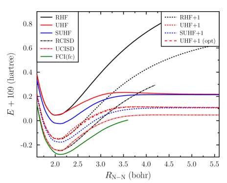
Figure 4: Dissociation profile of the N₂ molecule evaluated with various methods and the cc-pVDZ basis set. RHF+1 indicates the energy after a single gd step starting from the RHF wavefunction. UHF+1 (opt) indicates that the functional $E_{1}$ of Eq. 10 is minimized using a trial wavefunction of UHF form. The FCI results, using the frozen-core approximation, are from Ref. Krogh and Olsen, 2001.

We emphasize that, in this case, we have produced the energies after a single gd step without a formal vector representation of the starting reference wavefunctions (in a basis of Slater determinants, the dimension of the FCI vector is $\approx 1.4\times 10^{12}$). In evaluating the energy after the single gd step we computed $\langle 0|H^{3}|0\rangle$ for a reference wavefunction that is either a single Slater determinant or a linear combination of non-orthogonal determinants. In both cases the evaluation can be completed, by making use of Wick’s theorem, with a computational effort of $\mathcal{O}(N^{3}M^{3})$ (with $N$ being the number of electrons and $M$ the number of virtual orbitals). For this system we do not show results after a second step as we do not currently have code that can evaluate up to $\langle 0|H^{5}|0\rangle$.

In the case of RHF, a single gd step recovers $\approx 50~{}\%$ of the correlation energy near equilibrium. Starting from the SUHF reference wavefunction we again recover $\approx 50~{}\%$ of the missing energy after a single gd step. As expected, RCISD and UCISD energies are significantly lower than RHF+1 and UHF+1, although the curves are quite parallel to each other.

As we have discussed above, $E_{1}$ (Eq. 10) is explicitly a functional of $|0\rangle$. We can therefore choose to optimize the parameters in $|0\rangle$ to minimize $E_{1}$, instead of $E_{0}$. We have done so with a UHF functional form, as shown in Fig. 4 under the label UHF+1 (opt). We note that, in setting up the optimization process, we evaluate the derivative of $E_{1}$ analytically, as explained in App. B. The gradient evaluation can still be carried out with a computational effort of $\mathcal{O}(N^{3}M^{3})$, i.e., the same scaling as for the energy. While in this case we only see a modest improvement associated with the minimization of $E_{1}$ directly, it can still be a valuable approach as this can simplify the evaluation of molecular properties expressed as energy derivatives.

We show in Tab. 1 the spectroscopic constants of N₂, O₂, and F₂, evaluated using the cc-pCVTZ basis set, from HF and SUHF calculations with and without the single gd step. In the case of N₂, the length of the FCI vector expressed in a basis of Slater determinants is $\approx 2.9\times 10^{19}$, far exceeding what is currently feasible with any current deterministic FCI code. We do not show results starting from a UHF reference wavefunction for O₂ (as UHF does not dissociate correctly) or F₂ (as the molecule is unbound with UHF). The SUHF calculations on O₂ use a reference determinant with $m_{s}=0$ (while still projecting to a triplet state) in order to reach the best possible dissociation limit.

The calculations shown in Tab. 1 are compared to high-quality internally contracted multi-reference CI (IC-MRCI) results from Ref. Peterson et al., 1997, as well as the experimental values compiled in the same reference. In all cases the single gd step yields improved spectroscopic constants over the results obtained with HF or SUHF. While the amount of the missing correlation recovered is modest in all cases (around $30\%$), it is still noteworthy given that a single gd step was performed. A better reference wavefunction or a further gd or qn step can significantly improve the results presented in Tab. 1.

Table 1: Spectroscopic constants ($E_{e}$ in hartree, $D_{e}$ in kcal/mol, $r_{e}$ in Å, and $\omega_{e}$ in cm^-1) of N₂, O₂, and F₂ computed with various methods using the cc-pCVTZ basis set.

	N2				O2				F2
method	$E_{e}$	$D_{e}$	$r_{e}$	$\omega_{e}$	$E_{e}$	$D_{e}$	$r_{e}$	$\omega_{e}$	$E_{e}$	$D_{e}$	$r_{e}$	$\omega_{e}$
HF	-108.987698	116.7	1.0660	2727.7
HF+1	-109.081335	124.2	1.0642	2719.9
SUHF	-109.057362	158.2	1.0909	2417.8	-149.675867	30.8	1.1566	1980.4	-198.851568	14.1	1.4803	663.9
SUHF+1	-109.146989	163.2	1.0880	2435.5	-149.777920	36.0	1.1541	1971.8	-198.961698	15.1	1.4709	676.6
IC-MRCI	-109.464001	220.0	1.1007	2350.7	-150.209357	112.6	1.2099	1575.0	-199.376661	32.3	1.4165	893.3
exptl		228.4	1.0977	2358.6		120.6	1.2075	1580.2		39.0	1.4119	916.6

IV Conclusions

In this work, we have considered gradient descent and quasi-Newton algorithms to reach the FCI ground state energy starting from an arbitrary reference wavefunction. The FCI ground state is systematically approached with increasing number of steps taken using either algorithm.

A central ingredient of this work is to avoid an explicit representation of the wavefunction, opting to write the energies, at each step in the optimization, as functionals of the reference wavefunction. The resulting functionals have some useful properties:

• They are independent of the form of the reference wavefunction. Therefore, they provide an unbiased way to compare how different wavefunctions evolve towards the FCI ground state along the optimization path.

• The functional forms are independent of the specific wavefunction parameters. That is to say, if the reference wavefunction is chosen as a single Slater determinant, then any Slater determinant (as long as it is not orthogonal to the FCI ground state) can be used with the functional forms provided.

While in this work we have focused on single determinant wavefunctions as well as linear combinations of non-orthogonal determinants, the evaluation of the required $\langle 0|H^{k}|0\rangle$ matrix elements can also be efficiently done (in polynomial time) for other types of wavefunctions such as multi-configuration self-consistent field (MC-SCF) or generalized valence-bond (GVB) expansions, to name a few. An efficient evaluation of the $\langle 0|H^{k}|0\rangle$ matrix elements avoids the storage of intermediate wavefunctions as explicit vectors over the Hilbert space, thus allowing the computation of energies along the optimization path for systems where the dimension of the Hilbert space is larger than the storage resources available.

Given that the evaluation of the matrix elements $\langle 0|H^{k}|0\rangle$ can become quite expensive as $k$ increases, we realize that practical applications may be limited to the first few steps. In this case, a better starting initial inverse Hessian (as opposed to $B=I$) can lead to substantially improved results. We are currently investigating this possibility.

Data Availability

The data that support the findings of this study are available from the corresponding author upon reasonable request.

Appendix A Search direction from BFGS update

We discuss in this appendix the form of the search direction $p_{1}=-B_{1}g_{1}$, with $B_{1}$ constructed from from a Broyden-Fletcher-Goldfarb-Shanno (BFGS) Broyden (1970); Fletcher (1970); Goldfarb (1970); Shanno (1970) update formula (starting from $B_{0}=I$).

Let

$$s_{0} \equiv\,Z_{1}-Z_{0}=Z_{1},$$ (22)

$$y_{0} \equiv\,g_{1}-g_{0},$$ (23)

which would yield $s_{0}=-\sigma_{\ast}g_{0}$ and $(y_{0})_{x}=(\alpha_{1}-\alpha_{0})H_{x}^{0}+\beta_{1}H_{x}^{y}H_{y}^{0}$. With $\rho_{0}=1/[(s_{0})^{x}(y_{0})_{x}]$, the BFGS update takes the form

$$(B_{1})_{s}^{t} =\,(B_{0})_{s}^{t}-\rho_{0}(B_{0})_{s}^{x}(y_{0})_{x}(s_{0})^{t}-\rho_{0}(s_{0})_{s}(y_{0})^{x}(B_{0})_{x}^{t}$$

$$+\,\rho_{0}^{2}\Big{[}\rho^{-1}_{0}+(y_{0})^{x}(B_{0})_{x}^{y}(y_{0})_{y}\Big{]}(s_{0})_{s}(s_{0})^{t}$$ (24)

We now carry an explicit evaluation of $p_{1}=-B_{1}g_{1}$. We note that

$$\rho^{-1}_{0} =\,-\sigma_{\ast}\alpha_{0}(\alpha_{1}-\alpha_{0})f_{2}-\sigma_{\ast}\alpha_{0}\beta_{1}f_{3},$$

$$[y_{0}y_{0}] \equiv\,(y_{0})^{x}(y_{0})_{x}$$

$$=\,(\alpha_{1}-\alpha_{0})^{2}f_{2}+2(\alpha_{1}-\alpha_{0})\beta_{1}f_{3}+\beta_{1}^{2}f_{4},$$

$$[s_{0}g_{1}] \equiv\,(s_{0})^{x}(g_{1})_{x}$$

$$=\,-\sigma_{\ast}\alpha_{0}\alpha_{1}f_{2}-\sigma_{\ast}\alpha_{0}\beta_{1}f_{3},$$

$$[y_{0}g_{1}] \equiv\,(y_{0})^{x}(g_{1})_{x}$$

$$=\,\alpha_{1}(\alpha_{1}-\alpha_{0})f_{2}-\alpha_{0}\beta_{1}f_{3}+\beta_{1}^{2}f_{4}.$$

Therefore, $p_{1}$ takes the form

$$(p_{1})_{x}=\alpha^{\prime}_{1}H_{x}^{0}+\beta^{\prime}_{1}H_{x}^{y}H_{y}^{0},$$ (25)

with

$$\alpha^{\prime}_{1} =\,\alpha_{1}-2\sigma_{\ast}\rho_{0}^{2}(\rho_{0}^{-1}+[y_{0}y_{0}])[s_{0}g_{1}]$$

$$-\,\rho_{0}(\alpha_{1}-\alpha_{0})[s_{0}g_{1}]+2\sigma_{\ast}\rho_{0}[y_{0}g_{1}],$$ (26)

$$\beta^{\prime}_{1} =\,\beta_{1}-\rho_{0}\beta_{1}[s_{0}g_{1}].$$ (27)

Appendix B Optimization of $E_{1}$ with a Slater determinant

In this section we consider the optimization of the $E_{1}$ functional of Eq. 10 using a Slater determinant trial wavefunction. A Slater determinant wavefunction $|\Phi\rangle$ can be parametrized in terms of Thouless rotations (see, e.g., Ref. Jiménez-Hoyos et al., 2012) as

$$|\Phi\rangle=\mathcal{N}\exp\left(\sum_{i}T_{ai}c^{\dagger}_{a}\,c_{i}\right)|\Phi_{0}\rangle,$$ (28)

where $\mathcal{N}$ is a normalization factor, $|\Phi_{0}\rangle$ is some initial reference Slater determinant, and $T_{ai}$ are Thouless amplitudes to be optimized. Here, indices $a$ and $i$ run over particle and holes, respectively.

The functional $E_{1}$ is fully expressed in terms of the expectation values $\langle 0|H|0\rangle$, $\langle 0|H^{2}|0\rangle$, and $\langle 0|H^{3}|0\rangle$. In assembling the gradient of $E_{1}$, it is sufficient to consider the gradients of those matrix elements. Consider the matrix element $\langle 0|H^{k}|0\rangle$, with $|0\rangle=|\Phi\rangle$ and $|\Phi\rangle$ written in the form of Eq. 28. The matrix element is given by

$$\frac{\langle\Phi|H^{k}|\Phi\rangle}{\langle\Phi|\Phi\rangle}\equiv\frac{\langle\Phi_{0}|\exp(T^{\dagger})\,H^{k}\exp(T)|\Phi_{0}\rangle}{\langle\Phi_{0}|\exp(T^{\dagger})\,\exp(T)|\Phi_{0}\rangle}.$$ (29)

Explicit differentiation of the equation above yields

$$\left.\frac{\partial}{\partial T_{ai}^{\ast}}\frac{\langle\Phi|H^{k}|\Phi\rangle}{\langle\Phi|\Phi\rangle}\right|_{T=0}=\frac{\langle\Phi_{0}|c^{\dagger}_{i}\,c_{a}H^{k}|\Phi_{0}\rangle}{\langle\Phi_{0}|\Phi_{0}\rangle}.$$ (30)

We finally note that the evaluation of $\langle\Phi|H^{k}|\Phi\rangle$ and its derivatives, with $|0\rangle$ chosen as a Slater determinant, can be carried out by use of Wick’s theorem.

References

- Szabo and Ostlund (1989) A. Szabo and N. S. Ostlund, Modern Quantum Chemistry: Introduction to Advanced Electronic Structure Theory (McGraw-Hill, New York, 1989).
- Davidson (1975) E. R. Davidson, J. Comput. Phys. 17, 87 (1975).
- Sundstrom and Head-Gordon (2014) E. J. Sundstrom and M. Head-Gordon, J. Chem. Phys. 140, 114103 (2014).
- Jiménez-Hoyos et al. (2012) C. A. Jiménez-Hoyos, T. M. Henderson, T. Tsuchimochi, and G. E. Scuseria, J. Chem. Phys. 136, 164109 (2012).
- Wang et al. (2019) Z. Wang, Y. Li, and J. Lu, J. Chem. Theory Comput. 15, 3558 (2019).
- Wolfe (1969) P. Wolfe, SIAM Review 11, 226 (1969).
- Wolfe (1971) P. Wolfe, SIAM Review 13, 185 (1971).
- Nakatsuji (2012) H. Nakatsuji, Acc. Chem. Res. 45, 1480 (2012).
- Nocedal and Wright (2006) J. Nocedal and S. J. Wright, Numerical Optimization (Springer, New York, 2006), 2nd ed.
- Broyden (1970) C. G. Broyden, IMA J. Appl. Math. 6, 76 (1970).
- Fletcher (1970) R. Fletcher, Comput. J. 13, 317 (1970).
- Goldfarb (1970) D. Goldfarb, Math. Comp. 24, 23 (1970).
- Shanno (1970) D. F. Shanno, Math. Comp. 24, 647 (1970).
- Qiu et al. (2017) Y. Qiu, T. M. Henderson, and G. E. Scuseria, J. Chem. Phys. 146, 184105 (2017).
- Krogh and Olsen (2001) J. W. Krogh and J. Olsen, Chem. Phys. Lett. 344, 578 (2001).
- Frisch et al. (2016) M. J. Frisch, G. W. Trucks, H. B. Schlegel, G. E. Scuseria, M. A. Robb, J. R. Cheeseman, G. Scalmani, V. Barone, G. A. Petersson, H. Nakatsuji, et al., Gaussian 16 Revision C.01 (2016), Gaussian Inc., Wallingford, CT.
- Peterson et al. (1997) K. A. Peterson, A. K. Wilson, D. E. Woon, and T. H. Dunning, Jr., Theor. Chem. Acta 97, 251 (1997).
- Jiménez-Hoyos et al. (2012) C. A. Jiménez-Hoyos, R. Rodríguez-Guzmán, and G. E. Scuseria, Phys. Rev. A 86, 052102 (2012).