Abstract

Inflation driven by a generic self-gravitating medium is an interesting alternative to study the impact of spontaneous spacetime symmetry breaking during a quasi de-Sitter phase, in particular the 4-dimensional diffeomorphism invariance of GR is spontaneously broken down to $ISO(3)$. The effective description is based on four scalar fields that describe the excitations of a supersolid. There are two phonon-like propagating scalar degrees of freedom that mix non-trivially both at early and late times and, after exiting the horizon, give rise to non-trivial correlations among the different scalar power spectra. The non-linear structure of the theory allows a secondary gravitational waves production during inflation, efficient enough to saturate the present experimental bound and with a blue-tilted spectral index.

1 Introduction

Inflation is the most compelling way to solve the drawbacks of the hot big bang model and simultaneously generate the seed of the primordial perturbations to be used as initial conditions for the latter stages of Universe’s evolution. The simplest class of models is single clock inflation, where time diffeomorphisms are non-linearly realized, whose predictions are largely independent on how the Universe is reheated. Indeed, according to the Weinberg theorem on cosmological perturbations [1, 2], at large scales and under mild assumptions, the curvature perturbations of the constant density hypersurfaces $\zeta$, or equivalently the comoving curvature ${\cal R}$, are conserved and can be used to set the primordial initial conditions for the scalar sector at the beginning of radiation domination. The situation is different for models characterized by different symmetry breaking patterns, featuring more degrees of freedom for which the Weinberg theorem does not hold. In this case, ${\cal R}$ and $\zeta$ are not conserved and ${\cal R}\neq\zeta$ at superhorizon scales; thus, the details of reheating have to be taken into account [3, 4, 5, 6, 7]. That is exactly what happens when a fluid [8] or solid [9] drives inflation. In this work, we present an effective field theory (EFT) description suitable to describe the complete breaking of spacetime diffeomorphisms during inflation by using the minimal set of four scalar fields $\{\varphi^{A}\,,\;A=0,1,2,3\}$ sporting a suitable set of internal symmetries. As a matter of fact, $\varphi^{A}$ can also be interpreted as the coordinates of a self-gravitating non-dissipative medium [10, 11, 12, 13, 14, 15] that in our case is a supersolid. A complete analysis of the linear evolution of scalar and tensor modes, together with the computation of the corresponding power spectra is given. In addition, we consider the secondary production of gravitational waves (GWs) during inflation, exploiting the cubic vertex of the theory involving a tensor and two scalars, saturating the experimental bound set by Planck without upsetting the scalar 3-point function. The secondary production can give a blue tilt to the spectral index, an important feature for the direct detection of the stochastic GWs background produced during inflation. A detailed analysis of non-Gaussianity can be found in a companion paper [16].

The outline of the paper is the following. In section 2 we briefly review the effective field theory description of a supersolid at the leading order in derivates. In section 3, the dynamics of the two independent scalar perturbations are careful analyzed both at classical and quantum level, computing the relevant scalar power spectra and constraining the parameter region by using Plank data. Section 4 is devoted to study, in the instantaneous reheating approximation, how the seed of primordial perturbations are transmitted to the radiation dominated phase in a $\Lambda$CDM universe. In section 6 primary and secondary gravitational waves production during inflation is considered. Our conclusions are drawn in section 7.

2 Supersolids and Inflation

Several features of inflationary models can be traced back to the spontaneous symmetry breaking pattern: in single field inflation, the non-trivial time-dependent configuration of the inflaton breaks time reparametrization leaving unbroken the space diffeomorphisms of the $t=$const. hypersurface. However, there are other possibilities. For instance, an inflationary model where spatial diffeomorphisms are non-linearly realized was studied in [9] by working with three scalar fields. In a similar fashion, one can consider a more general case in which all diffeomorphisms are broken by the background configuration of four scalar fields

$$\varphi^{0}=\bar{\varphi}(t)\,,\qquad\qquad\varphi^{i}=x^{i}\,$$ (2.1)

which will be the background configuration for the inflationary phase. The existence of a spatially homogeneous background is allowed by the presence of global symmetries of the scalar field action. Consider a special multi-field model of inflation based on four scalar fields $\varphi^{A}$, $A=0\,,1\,,\,2\,,\,3$ with shift symmetry [11, 15]

$$\varphi^{A}\rightarrow\varphi^{A}+c^{A}\,,$$ (2.2)

and $SO(3)$ internal symmetry

$$\varphi^{a}\to{\varphi^{\prime}}^{a}={\cal R}^{a}_{b}\;\varphi^{a}\,,\qquad a=1,2,3\qquad\qquad{\cal R}^{t}\;{\cal R}=1\,.$$ (2.3)

The “vacuum” configuration (2.1) has a residual global “diagonal” $ISO(3)$ symmetry. Indeed, a global spatial rotation ${\cal R}^{i}_{j}x^{j}$ can be absorbed by a corresponding inverse internal transformation of $\varphi^{a}$ and the same is true for a global translation $x^{i}\to x^{i}+c^{i}$ thanks to the shift symmetry (2.2). Among the spacetime scalars shift symmetric operators with a single derivative of $\varphi^{A}$

$$C^{AB}=g^{\mu\nu}\partial_{\mu}\varphi^{A}\,\partial_{\nu}\varphi^{B}\;\;\qquad A,B=0,1,2,3\,,$$ (2.4)

one can extract 10 operators invariant under internal $SO(3)$ rotations (2.3)

$$\begin{split}&b=\sqrt{\text{Det}\left[\textbf{B}\right]}\,,\qquad\varsigma=\sqrt{\text{Det}\left[\textbf{W}\right]}\,,\qquad y=u^{\mu}\,\partial_{\mu}\varphi^{0}\,,\qquad\chi=\sqrt{-C^{00}}\,,\\ &\tau_{X}=\text{Tr}\left[\textbf{B}\right]\,,\qquad\tau_{Y}=\frac{\text{Tr}\left[\textbf{B}^{2}\right]}{\tau_{X}{}^{2}}\,,\qquad\tau_{Z}=\frac{\text{Tr}\left[\textbf{B}^{3}\right]}{\tau_{X}{}^{3}}\,,\\ &w_{X}=\text{Tr}\left[\textbf{W}\right]\,,\qquad w_{Y}=\frac{\text{Tr}\left[\textbf{W}^{2}\right]}{w_{X}{}^{2}}\,,\qquad w_{Z}=\frac{\text{Tr}\left[\textbf{W}^{3}\right]}{w_{X}{}^{3}}\,;\end{split}$$ (2.5)

where

$$u^{\mu}=-\frac{\epsilon^{\mu\nu\alpha\beta}}{6\;b\;\sqrt{-g}}\,\epsilon_{abc}\;\partial_{\mu}\varphi^{a}\,\partial_{\nu}\varphi^{b}\,\partial_{\beta}\varphi^{c}\,,\qquad u^{2}=-1\,,$$ (2.6)

plays the role of the medium four-velocity such that $u^{\mu}\partial_{\mu}\varphi^{a}=0$ and

$$B^{ab}=C^{ab}\,,\qquad\qquad W^{ab}=B^{ab}-\frac{C^{0a}\,C^{0b}}{C^{00}}\,,\qquad a=1,\,2,\,3\,.$$ (2.7)

By using the relation $\varsigma=\chi^{-1}\,b\,y$ and the Cayley-Hamilton theorem, only $7$ among those operators are independent. Thus, we arrive at the action

$$S=\frac{M_{\text{Pl}}^{2}}{2}\,\int dx^{4}\,\sqrt{-g}\,R+M_{\text{Pl}}^{2}\,\int dx^{4}\,\sqrt{-g}\,U(b,\,y,\,\chi,\,\tau_{Y},\,\tau_{Z},\,w_{Y},\,w_{Z})\,,$$ (2.8)

that can be interpreted as the relativistic generalization of the low-energy effective Lagrangian describing homogeneous and isotropic supersolids at zero-temperature [17, 18]. Such an action is the most general at leading order in a derivative expansion compatible with (2.2) and (2.3) and it is rather useful to study systematically the symmetry breaking pattern of spacetime symmetry during inflation.

By inspection of the energy momentum tensor (EMT), the energy density and the pressure are given by

$$\rho=M_{\text{Pl}}^{2}\,\left(-U+\chi\,U_{\chi}+y\,U_{y}\right)\,,$$ (2.9)

$$p=M_{\text{Pl}}^{2}\,\left(U-b\,U_{b}\right)\,.$$ (2.10)

According to the Noether theorem, there are four conserved currents:

$$J^{\mu}_{A}=2\,M_{\text{Pl}}^{2}\,\frac{\partial U}{\partial C^{AB}}\nabla^{\mu}\varphi^{B}\,;$$ (2.11)

three related to solid configurations that spontaneously break translation invariance and one associated with the superfluid frictionless flow. In particular, the particle number density $n_{sf}$ of the superfluid component can be expressed in terms of the Noether current $J^{0}_{\mu}$ as

$$n_{sf}=-u^{\alpha}\,J_{\alpha}^{0}\,;$$ (2.12)

while the density of lattice sites $n_{\ell}$ is identified as the projection of the off shell conserved current  $J_{\alpha}=b\,u_{\alpha}$ along the four-velocity $u^{\mu}$, namely [17]

$$n_{\ell}=-u_{\alpha}\,J^{\alpha}=b\,.$$ (2.13)

This allows us to define the superfluid density per lattice site $\sigma$ as

$$\sigma=\frac{n_{sf}}{n_{\ell}}=\frac{M_{\text{Pl}}^{2}}{b}\left(U_{y}+\frac{y}{\chi}\,U_{\chi}\right)\,.$$ (2.14)

As we will see, at cosmological level, the perturbations $\delta\sigma$ generate non-adiabatic contributions (for this reason, we will regard $\delta\sigma$ in the following as an isocurvature or entropic perturbation). Similarly, for the rest of the paper we identify $n_{\ell}$ (2.13) with the usual particle density $n$.
While $u^{\mu}$ represents the 4-velocity of the normal component of the supersolid,

$${\cal V}_{\mu}=\frac{\partial_{\nu}\varphi^{0}}{\chi}$$ (2.15)

is the 4-velocity (irrotational) of the superfluid component.

One of the key features is that two independent phonon-like excitations are present. In general, the supersolid perturbation can be written around a flat space-time as

$$g_{\mu\nu}=\eta_{\mu\nu},\qquad\varphi^{0}=t+\pi_{0}\,,\qquad\varphi^{i}=x^{i}+\partial^{i}\pi_{L}+\pi_{T}^{i}\,,\qquad\partial_{i}\pi_{T}^{i}=0\,.$$ (2.16)

At the quadratic level, we have [19]

$${\cal S}^{(2)} =\int d^{4}x\Big{[}\frac{(\hat{M_{1}}+\bar{\rho}+\bar{p})}{2}\,\partial_{t}\pi_{L}\,\Delta\,\partial_{t}\pi_{L}+\left(\hat{M}_{3}-\hat{M}_{2}\right)\pi_{L}\,\Delta^{2}\,\pi_{L}+\hat{M}_{0}\,{\pi_{0}^{\prime}}^{2}+\left(2\,\hat{M}_{4}-\hat{M}_{1}\right)\pi_{0}^{\prime}\Delta\pi_{l}$$

$$-\frac{\hat{M}_{1}}{2}\pi_{0}\,\Delta\,\pi_{0}+\frac{(\hat{M}_{1}+\bar{\rho}+\bar{p})}{2}\,\partial_{t}\pi_{T}^{i}\,\partial_{t}\pi_{T}^{i}-\frac{\hat{M}_{2}}{2}\pi_{T}^{i}\,\Delta\,\pi_{T}^{i}\Big{]}\,;$$

where $\bar{\rho}$ and $\bar{p}$ are the background values of the energy density and pressure (constant in space and time) while $\Delta=\delta_{ij}\partial_{i}\partial_{j}$; finally, the derivative of a function $f$ with respect to conformal time is denoted by $f^{\prime}$. The parameters $\hat{M}_{a}=M_{\text{Pl}}^{2}\,M_{a}$ are proportional to first and second derivatives of $U$ and are given in appendix A. Notice that the space shift symmetry is crucial to have a homogeneous EMT even if the scalar fields have non-trivial background values.
The properties of the EMT are largely determined by the symmetries of $U$ as discussed in [14, 15]. It is useful to summarize the main features associated with the presence or absence of some of the operators (and the related mass parameters) in the Lagrangian depending on a specific set of internal symmetries.

• Perfect Fluids:

  • $U(b):$ only $\{\varphi^{a}\,,\;\;a=1,2,3\}$ are present; the Lagrangian is invariant under internal volume preserving diffeomorphisms $V_{s}\text{Diff}$: $\varphi^{a}\to\Psi^{a}(\varphi^{b})$ , $\det|\partial\Psi^{a}/\partial{\varphi^{b}}|=1$, $a,b=1,2,3$.

  • $U(\chi)$: it is the most general Lagrangian for a perfect irrotational fluid with $\varphi^{0}$ only.

  • $U(b,\,y)$: the most general isentropic perfect fluid; the Lagrangian is invariant under $V_{s}\text{Diff}$ and $\varphi^{0}\to\varphi^{0}+f(\varphi^{a})$.

• Superfluids $U(b,\,y,\,\chi)$: invariant under volume preserving diffeomorphisms $V_{s}\text{Diff}$.

• Solids $U(b,\,\tau_{Y},\,\,\tau_{Z})$: is the most general Lagrangian with only $\{\varphi^{a}\,,\;\;a=1,2,3\}$ present.

• Zero-Temperature Supersolids $U(b,\,y,\,\chi,\,\tau_{Y},\,\,\tau_{Z},\,w_{Y},\,w_{Z})$.

As a remark, in the literature solids are typically associated with the presence of only three scalar fields $\{\varphi^{a}\,,a=1,2,3\}$ and a Lagrangian of the form $U(\tau_{X},\tau_{Y},\tau_{Z})$, see for instance [9]. However, introducing a fourth scalar $\varphi^{0}$ and enforcing the following field dependent shift symmetry

$$\varphi^{0}\to\varphi^{0}+f(\varphi^{a})\,,$$ (2.17)

the allowed operators are $b$, $\tau_{Y}$, $\tau_{Z}$ and $y$ and the resulting theory $U(b,\,\tau_{Y},\,\tau_{Z},\,y)$ describes an adiabatic solid in the sense that the entropic perturbation $\delta\sigma$ is a conserved quantity as discussed in [15, 20]. The term supersolid is reserved to the case where, in addition to the phonons of the solid, also the entropic perturbation $\delta\sigma$ propagates.

A more detailed analysis of thermodynamical properties for general supersolids is planned for a future work. Finally, stability of (2) imposes the following conditions [19]

$$\hat{M}_{0}>0\,,\qquad-(\bar{p}+\bar{\rho})<\hat{M}_{1}<0\,,\qquad\hat{M}_{2}>0\,,\qquad\hat{M}_{2}>\hat{M}_{3}\,.$$ (2.18)

As we will see, such conditions are necessary for the existence of the Bunch-Davies (BD) vacuum in an inflating phase driven by a supersolid. During a quasi deSitter period, the most convenient parametrization of the mass term is through some $c_{i}^{2}$ parameters such that

$$M_{i}\equiv M_{\text{Pl}}^{-2}\;(1+w)\;\rho\;c_{i}^{2}\qquad i=0,1,2,3,4\,.$$ (2.19)

(where $w$ is defined in (3.5)) with the assumption that $c_{i}^{2}$ are slowly varying in time ($\frac{c_{i}^{\prime}}{{\cal H}\,c_{i}}\ll 1$).

3 Slow-roll

Cosmological perturbations in the flat-slice gauge are described by

$$\begin{split}&\varphi^{0}=\bar{\varphi}(t)+\pi_{0}\,,\qquad\varphi^{i}=x^{i}+\partial^{i}\pi_{L}+\pi_{T}^{i}\,,\qquad\partial_{i}\pi_{T}^{i}=0\,,\\ &ds^{2}=a^{2}\left[(2\,\Psi-1)\;dt^{2}+2\,dt\;dx^{i}\,\partial_{i}F+\delta_{ij}\;dx^{i}\;dx^{j}\right]\,.\end{split}$$ (3.1)

Perturbations in a generic gauge are discussed in Appendix B. The background EMT tensor has the form of the one of a perfect fluid with energy density and pressure given by (2.9) and (2.10) evaluated on FLRW; the conservation of the background EMT is equivalent to 

$$\bar{\varphi}^{\prime\prime}={\cal H}\,(1-3\,c_{b}^{2})\;\bar{\varphi}^{\prime}\,,$$ (3.2)

where

$$c_{b}^{2}=-\frac{c_{4}^{2}}{c_{0}^{2}}\,.$$ (3.3)

For $c_{b}^{2}$ constant in time, we have

$$\bar{\varphi}^{\prime}=\bar{\varphi}^{\prime}_{0}\;a^{1-3\;c_{b}^{2}},\qquad\bar{\varphi}^{\prime}_{0}=const$$ (3.4)

Our benchmark values for $c_{b}^{2}$ will be $c_{b}^{2}=0$ which gives $\bar{\varphi}^{\prime}=a\;\bar{\varphi}^{\prime}_{0}$, and $c_{b}^{2}=-1$ leading to $\bar{\varphi}^{\prime}=\bar{\varphi}^{\prime}_{0}\;a^{-4}$. Inflation takes place when

$$w<-\frac{1}{3}\,,\qquad w=\frac{\bar{p}}{\bar{\rho}}\,.$$ (3.5)

We will be mainly interested in slow-roll (SR) inflation  for which the following dynamical parameters are small

$$\epsilon=1-\frac{{\cal H}^{\prime}}{{\cal H}^{2}}=\frac{3}{2}\,(1+w)\,,\qquad\qquad\eta=\frac{\epsilon^{\prime}}{\epsilon\,{\cal H}}\ll 1\,.$$ (3.6)

Note that in a quasi dS phase, the adiabatic speed of sound is given by

$$c_{s}^{2}=\frac{p^{\prime}}{\rho^{\prime}}=\frac{2}{3}\left(3\,c_{0}^{2}\,c_{b}^{4}+c_{2}^{2}-3\,c_{3}^{2}\right)=-1+\frac{2}{3}\,\epsilon-\frac{1}{3}\,\eta\,{}_{|\text{SR}}\simeq-1.$$ (3.7)

Both $\Psi$ and $F$ are non-dynamical fields and their linear equations of motion can be solved in terms of $\pi_{0}$ and $\pi_{L}$, at the leading order in SR and working in Fourier space, one finds

$$\begin{split}&\Psi=\frac{c_{1}^{2}\,\mathcal{H}\,\epsilon}{\bar{\varphi}^{\prime}}\pi_{0}-\mathcal{H}\epsilon\,\left(c_{1}^{2}+1\right)\,\pi_{L}^{\prime}\,;\\ &F={\cal H}\,(2\,c_{0}^{2}\,c_{b}^{2}-1)\,\pi_{L}\,\epsilon-3\,c_{1}^{2}\,k^{-2}\,{\cal H}^{2}\,\frac{\pi_{0}}{\bar{\varphi}^{\prime}}\,\epsilon+3\,(1+c_{1}^{2})\,{\cal H}^{2}\,k^{-2}\,\pi_{L}^{\prime}\,\epsilon+2\,c_{0}^{2}\,k^{-2}\,{\cal H}\,\frac{\pi_{0}^{\prime}}{\bar{\varphi}^{\prime}}\,\epsilon\,;\end{split}$$ (3.8)

The following action describes the linear dynamics at the leading order of a slow-roll expansion in $\epsilon$:

$$S_{2}\equiv\int dt\;d^{3}k\;\left(\frac{1}{2}{\pi^{\prime}}^{t}\,{\cal K}\,\pi^{\prime}+{\pi^{\prime}}^{t}\,{\cal D}_{\pi}\,\pi-\frac{1}{2}\pi^{t}\,{\cal M}_{\pi}\,\pi\right)\,,\quad\quad\pi=\begin{pmatrix}\pi_{L}\\ \pi_{0}\end{pmatrix}\,;$$ (3.9)

with

$${\cal K}=M_{\text{Pl}}^{2}\,\mathcal{H}^{2}\,a^{2}\,\epsilon\left(\begin{array}[]{cc}4\,\left(1+c_{1}^{2}\right)\,k^{2}&0\\ 0&8\,\,c_{0}^{2}\;\bar{\varphi}^{\prime}{}^{-2}\end{array}\right)\,,$$ (3.12)

$${\cal D}_{\pi}=-\frac{2\,a^{2}\,k^{2}\,M_{\text{Pl}}^{2}\,\mathcal{H}^{2}\,\epsilon\,\left(2\,c_{0}^{2}\,c_{b}^{2}+c_{1}^{2}\right)}{\bar{\varphi}^{\prime}}\begin{pmatrix}0&1\\ -1&0\end{pmatrix}\,,$$ (3.13)

$${\cal M}_{\pi}=4\,M_{\text{Pl}}^{2}\,a^{2}\,\mathcal{H}^{2}\,k^{2}\,\epsilon\left(\begin{array}[]{cc}k^{2}\left(-1+\frac{4}{3}\,c_{2}^{2}-2\,c_{0}^{2}\,c_{b}^{4}\right)&-\frac{3\,\mathcal{H}\,\left(c_{1}^{2}-2\,c_{0}^{2}\,c_{b}^{2}\right)\,\left(1+\,c_{b}^{2}\right)}{2\;\bar{\varphi}^{\prime}}\\ -\frac{3\,\mathcal{H}\,\left(c_{1}^{2}-2\,c_{0}^{2}\,c_{b}^{2}\right)\,\left(1+\,c_{b}^{2}\right)}{2\;\bar{\varphi}^{\prime}}&-\frac{c_{1}^{2}}{\bar{\varphi}^{\prime}{}^{2}}\\ \end{array}\right)\,.$$ (3.16)

Up to boundary terms, one can always take ${\cal D}$ antisymmetric. The peculiarity of (3.9) is the mixing of the two propagating DoF (degrees of freedom) present at kinetic level due to the matrix ${\cal D}$ and at mass level being the matrix ${\cal M}$ non-diagonal. Such mixing is unavoidable unless the parameters $c_{b}$ and $c_{2}^{2}$, $c_{1}^{2}$ are unnaturally tuned, and it is a key property of a superfluid component in the solid at the origin of cross-correlations in the two and three points function of any scalar perturbation. As a result, the study of scalar linear perturbations is a bit involved and to get rid of the mixing by a suitable field redefinition few steps are needed. A similar system of coupled modes, described by (3.9), was encountered when studying the non-thermal production of gravitinos [22], multi-field inflation [23], chromo-natural inflation [24, 25] and in effective theories of inflation[21]. As far as we know, our analysis is the first complete one that does not rely on special choices of parameters.
The strategy to quantize the quadratic action will be the following. We start from the original fields $\pi_{0,L}$ that describe physically two Nambu-Goldstone modes around a non-trivial Lorentz breaking background solution. The quadratic action controlling the dynamics of such modes (3.9) exhibits both kinetic (the presence of ${\cal D})$ and mass mixing effects (non-diagonal ${\cal M}$). A similar kinetic mixing is also encountered in mechanical systems with gyroscopic forces like the Coriolis force or in the presence of magnetic fields; it is worth to stress that the ${\cal D}$ mixing can take place when at least two fields are present. The first step is to make the fields canonical by a time-dependent field redefinition $\Pi={\cal K}^{1/2}\;\pi$ (3.21). At this level the corresponding Lagrangian $L(\Pi,\;\Pi^{\prime})$ (3.22) is characterized by non trivial ${\cal D}-mixing$ and a time-dependent non diagonal mass matrix. The classical equations of motion correspond to a coupled system of second-order equations or, alternatively, to two decoupled fourth-order differential equations.

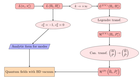
Figure 1: Schematic procedure for quantization

The quantization of the system goes through the choice of the BD by studying the Lagrangian in the UV ($k\to\infty$) regime (C.1) where $k$ dominates over all other scales. In this regime the mass term is diagonal and time independent. Thanks to this feature we can write a decoupled system of quantum oscillators and quantize it with the usual canonical rules in Hamiltonian formalism ($L(\Pi,\;\Pi^{\prime})\to L^{(UV)}(\Pi,\;\Pi^{\prime})\to{\cal H}^{(UV)}(\Pi,\;P)$) (C.3). The quantum oscillator dynamics is recovered by a canonical transformation at Hamiltonian level (involving also the conjugate momenta) ${\cal H}^{(UV)}(\Pi,\;P)\to{\cal H}^{(UV)}_{diagonal}(\tilde{\Pi},\;\tilde{P})$ (C.8). Introducing the Hamiltonian formalism allows us to decouple the two DoF with a canonical transformation and to select the BD vacuum. The main steps are summarized in Figure 1.

3.1 Quantization and Power Spectra

In order to define the Power Spectrum (PS) of a general quantum scalar field $\xi(\textbf{x})$, in Fourier space we set

$$\xi(\textbf{x})=\frac{1}{(2\,\pi)^{3}}\int\,d^{3}k\,e^{i\,\textbf{k}\cdot\textbf{x}}\,\xi_{\textbf{k}}\,,\qquad\xi_{\textbf{k}}=\sum_{i=1}^{2}\,\xi_{k}^{(cl)\,(i)}\,a_{\textbf{k}}{}^{(i)}+\xi_{k}^{(cl)\,(i)\,*}\,a_{-\textbf{k}}^{\dagger\,(i)}\,,$$ (3.17)

where the (cl) subscript stands for classic solution, and the latin index $i=1,\,2$ indicates the two indepedent scalar modes whose annihilation and creation operators obey the standard canonical commutation relations

$$\left[a^{(i)}_{\textbf{k}},\,a^{\dagger}_{\textbf{p}}{}^{(j)}\right]=(2\,\pi)^{3}\,\delta(\textbf{k}-\textbf{p})\,\delta^{i}_{j}\,.$$ (3.18)

Thus, the $\xi$ 2-point function reads

$$\langle\xi_{\textbf{k}}\,\xi_{\textbf{p}}\rangle=(2\,\pi)^{3}\,P_{\xi}(k)\,\delta(\textbf{k}+\textbf{p})\,,$$ (3.19)

and the $\xi$ scale-invariant PS is defined by

$$\begin{split}{\cal P}_{\xi}=\frac{k^{3}}{(2\,\pi^{2})}\,P_{\xi}&\equiv\frac{k^{3}}{(2\,\pi^{2})}\left(|\xi_{k}^{(cl)\,(1)}|^{2}+|\xi_{k}^{(cl)\,(2)}|^{2}\right)\\ &={\cal P}_{\xi}{}^{(1)}+{\cal P}_{\xi}{}^{(2)}\,.\end{split}$$ (3.20)

The first step to compute quantum correlators during inflation is to introduce the canonical field $\Pi$ defined by

$$\Pi\equiv\begin{pmatrix}\Pi_{L}\\ \Pi_{0}\end{pmatrix}={\cal K}^{1/2}\begin{pmatrix}\pi_{L}\\ \pi_{0}\end{pmatrix}\,.$$ (3.21)

The conditions (2.18) guarantee that the matrix ${\cal K}$ is positive definite. Given that the matrix elements of ${\cal K}$ are time-dependent, besides turning the kinetic term into a canonical one, the transformation (3.21) also alters the form of ${\cal D}$ and ${\cal M}$; thus, the quadratic Lagrangian in (3.9), when written in function of the new canonical fields becomes

$$L_{2}=\frac{1}{2}\Pi^{\prime}{}^{t}\Pi^{\prime}-\Pi^{t}\,{\cal D}\,\Pi^{\prime}-\frac{1}{2}\Pi^{t}\,{\cal M}\,\Pi\;;$$ (3.22)

where

$${\cal D}=k\,d\,\begin{pmatrix}0&-1\\ 1&0\end{pmatrix}\,,\qquad d=\frac{c_{1}^{2}+2\,c_{0}^{2}\;c_{b}^{2}}{2\,\sqrt{2\,c_{0}^{2}\,(1+c_{1}^{2})}}\,;$$ (3.23)

$${\cal M}=\begin{pmatrix}k^{2}\,\lambda_{L}{}^{2}-6\,{\cal H}^{2}&k\,{\cal H}\,\lambda\\ k\,{\cal H}\,\lambda&k^{2}\,\lambda_{0}{}^{2}-(1+3\,c_{b}^{2})(2+3\,c_{b}^{2})\,{\cal H}^{2}\end{pmatrix}\,,$$ (3.24)

$$\lambda_{L}^{2}=\frac{c_{L}^{2}-2c_{0}^{2}\,c_{b}^{4}}{1+c_{1}^{2}}\,,\qquad\lambda_{0}^{2}=-\frac{c_{1}^{2}}{2\,c_{0}^{2}}\,,\qquad\lambda=\frac{2^{1/2}\left[c_{0}^{2}\,c_{b}^{2}\,(1+3\,c_{b}^{2})-c_{1}^{2}\right]}{\sqrt{c_{0}^{2}\,(1+c_{1}^{2})}}\,,$$ (3.25)

and we have defined

$$c_{L}^{2}=-1+\frac{4}{3}\,c_{2}^{2}\,.$$ (3.26)

At the leading order in slow-roll, the equations of motion are the following

$$\begin{split}&\Pi_{L}{}^{\prime\prime}-2\,k\,d\Pi_{0}^{\prime}+\Pi_{0}\,k\,{\cal H}\,\lambda+\Pi_{L}\,\left(k^{2}\,\lambda_{L}^{2}-6\,{\cal H}^{2}\right)=0\,,\\ &\Pi_{0}{}^{\prime\prime}+2\,k\,d\Pi_{L}^{\prime}+\Pi_{L}\,k\,{\cal H}\,\lambda+\Pi_{0}\,\left(k^{2}\,\lambda_{0}^{2}-(1+3\,c_{b}^{2})\,(2+3\,c_{b}^{2})\,{\cal H}^{2}\right)=0\,.\end{split}$$ (3.27)

In order to quantize (3.22), we need to remove the kinetic mixing introduced by ${\cal D}$. Our strategy is the following: in the UV, at very large $k$, ${\cal M}$ becomes diagonal and time-independent. Thus, at very large $k$, the original Lagrangian (3.22) is equivalent to $L_{2}^{(\text{UV})}$, in accordance with the equivalence principle. In that regime, by using a canonical transformation, one can reduce the Hamiltonian associated to $L_{2}^{(\text{UV})}$ to a system of two canonical free fields $\tilde{\Pi}=(\tilde{\Pi}_{L},\,\tilde{\Pi}_{0})$ linearly related to $\Pi$

$$L_{2}^{(\text{UV})}=\frac{1}{2}\tilde{\Pi}^{\prime}{}^{t}\tilde{\Pi}^{\prime}-\frac{1}{2}\tilde{\Pi}^{t}\begin{pmatrix}k^{2}\,c_{s1}^{2}&0\\ 0&k^{2}\,c_{s2}^{2}\end{pmatrix}\tilde{\Pi}\,.$$ (3.28)

Thus, the unique Fock space vacuum is the BD vacuum for the system. Details can be found in Appendix C. The existence of the BD vacuum requires the frequencies squared $\left\{\omega^{2}_{1}=k^{2}\,c_{s1}^{2}\,,\;\omega^{2}_{2}=k^{2}\,c_{s2}^{2}\right\}$ to be strictly positive or equivalently $c^{2}_{si}>0\,,\;i=1,2$. In addition we restrict ourselves to the case of subluminal “diagonal” sound speeds: $0<c_{si}^{2}<1$. The conditions (2.18) are sufficient to have $c_{si}^{2}>0$ and when expressed in terms of (2.19) gives 

$$c_{0}^{2}>0,\,\qquad-1<c_{1}^{2}<0\,,\qquad c_{L}^{2}>2\,c_{0}^{2}\,c_{b}^{4}\,.$$ (3.29)

We have checked that there is a large region of parameters $c_{i}$ where the stability conditions hold together with $c^{2}_{s1}\,,c^{2}_{s2}<1$; moreover in such a region, the first two conditions when rewritten in terms of $c_{s1}$ and $c_{s2}$, become

$$c^{2}_{s2}<c_{L}^{2}<c^{2}_{s1}\,,$$ (3.30)

where we choose the convention $c_{s2}<c_{s1}$. The equations of motion (3.27) constitute a coupled system of second order linear differential equations with time-dependent coefficients. Finding explicit solution is not an easy task; of course, one could solve the equations numerically. However, from a physical point of view, it is more transparent to quantize the system focusing on the following values of $c_{b}$: $c_{b}^{2}=-1$ and $c_{b}^{2}=0$ for which an analytic solution can be found. Neglecting SR corrections, the coupled system of second order equations can be written as two indepedent fourth order equations for $\Pi_{0,L}$.
Remarkably, the case $c_{b}^{2}=0$ and $c_{b}^{2}=-1$ gives the following identical equations valid if $c_{1}^{2}\neq 0$

$$\begin{split}&\Pi_{L}{}^{(4)}+\left(c_{s1}^{2}+c_{s2}^{2}-\frac{12}{x^{2}}\right)\,\Pi_{L}{}^{\prime\prime}+\frac{24}{x^{3}}\,\Pi_{L}{}^{\prime}+\left(c_{s1}^{2}\;c_{s2}^{2}-\frac{6}{x^{2}}\,(c_{s1}^{2}+c_{s2}^{2})\right)\,\Pi_{L}\,=0\,,\\ &\Pi_{0}{}^{(4)}+\left(c_{s1}^{2}+c_{s2}^{2}-\frac{4}{x^{2}}\right)\,\Pi_{0}{}^{\prime\prime}+\frac{8}{x^{3}}\,\Pi_{0}{}^{\prime}+\left(c_{s1}^{2}\,c_{s2}^{2}-\frac{2}{x^{2}}\,\left(c_{s1}^{2}+c_{s2}^{2}\right)-\frac{8}{x^{4}}\right)\,\Pi_{0}\,=0\,;\end{split}$$ (3.31)

with $x=-k\,t$. Note the presence in (3.31) of the symmetry: $c_{s1}^{2}\leftrightarrow c_{s2}^{2}$. Analytic solutions are possible due to the absence of the terms $\Pi_{i}^{(3)}$ in the evolution equations. The solutions can be written as a linear combination of Bessel functions of order $5/2$ and $3/2$; the integration constants are fixed by imposing that subhorizon, where $x\gg 1$, the solution that represents flat space modes matches the ones given in (C.13) and (C.14); such a choice is equivalent to select the BD vacuum. Thus, $\Pi_{L}$ and $\Pi_{0}$ are quantum free (Gaussian) fields given by

$$\begin{split}&\Pi_{L\,k}=-i\,\sum_{j=1}^{2}\,a_{\textbf{k}}^{(j)}\,C_{L}^{(j)}\,\sqrt{\frac{\pi}{2}}\,c_{s\,j}{}^{\frac{1}{2}}\,\sqrt{-k\,t}\;H^{(1)}_{\frac{5}{2}}\left(-c_{s\,j}\,k\,t\right)+\text{h.c.}\,,\\ &\Pi_{0\,k}=-\sum_{j=1}^{2}\,a_{\textbf{k}}^{(j)}\,C_{0}^{(j)}\,\sqrt{\frac{\pi}{2}}\,c_{s\,j}{}^{\frac{1}{2}}\,\sqrt{-k\,t}\;H^{(1)}_{\frac{3}{2}}\left(-c_{s\,j}\,k\,t\right)+\text{h.c.}\,;\end{split}$$ (3.32)

the expression for $\left\{C_{L}^{(j)}\,,C_{0}^{(j)}\,;j=1,2\right\}$ can be found in Appendix C and $a_{\textbf{k}}^{(j)}$ are the creation operators for the fields defined in eq.(C.11). In single field SR inflation, naturally two gauge invariant scalar quantities can be considered when studying the dynamics of superhorizon modes: the curvature $\zeta$ of the $\rho=$ const. hypersurface and the curvature ${\cal R}$ of hypersurface orthogonal to the scalar component of the fluid 3-velocity

$$\begin{split}&\zeta=\Phi+{\cal H}\frac{\delta\rho}{\bar{\rho}^{\prime}}\,;\\ &{\cal R}=\Phi+{\cal H}\,v.\end{split}$$ (3.33)

According to the Weinberg theorem [1], in standard single field inflation, both $\zeta$ and ${\cal R}$ are conserved and coincides at superhorizon scales; as a result, the power spectrum of primordial perturbations during inflation is given in terms of the Fourier transform of the 2-point function of $\zeta$ or equivalently of ${\cal R}$. In our case, the Weinberg theorem does not hold and, besides the above curvature perturbations, additional gauge invariant scalar perturbations can be considered. In particular the curvature $\zeta_{n}$ of constant particle number $n$-hypersurface ( keep in mind that $n=n_{\ell}$), (2.13)) and curvature of the $\varphi^{0}=$const. hypersurface; namely

$$\zeta_{n}=-\Phi+\frac{{\cal H}}{\bar{n}^{\prime}}\,\delta n\,,\qquad\qquad{\cal R}_{\pi_{0}}=-\Phi+\frac{{\cal H}}{\bar{\varphi}^{\prime}}\,\pi_{0}\,.$$ (3.34)

The comoving curvature ${\cal R}_{\pi_{0}}$ is related to the superfluid component (2.15). The expression of the various curvature perturbations in terms $\pi_{L}$ and $\pi_{0}$ in a generic gauge can be found in Appendix B. In the spatially-flat gauge (3.1) we have that

$$\zeta_{n}=\frac{k^{2}}{3}\pi_{L}\,,\qquad{\cal R}_{\pi_{0}}=\frac{\cal H}{\bar{\varphi}^{\prime}}\pi_{0}\,.$$ (3.35)

The uniform curvature perturbation $\zeta$ can be obtained from eq. (B.15) at leading order in SR

$$\zeta=\left(1-2\,c_{0}^{2}\,c_{b}^{2}\right)\zeta_{n}-\frac{2}{3}\,c_{0}^{2}\,\frac{\pi_{0}^{\prime}}{\bar{\varphi}^{\prime}};$$ (3.36)

and similarly, from eq. (B.14), for the comoving curvature

$${\cal R}=\frac{3\,{\cal H}\,(1+c_{1}^{2})}{k^{2}}\zeta_{n}^{\prime}-c_{1}^{2}\,{\cal R}_{\pi_{0}}\,.$$ (3.37)

As anticipated, by using (3.32), being ${\cal C}_{L/0}^{(j)}\propto k^{-\frac{1}{2}}$, the power spectra of $\zeta_{n}$, ${\cal R}_{\pi_{0}}$, $\zeta$ and ${\cal R}$ will be scale-free, up to SR corrections. Moreover, as shown in (B.14) and (B.15), $\zeta$ and ${\cal R}$ are linear combinations of $\zeta_{n}$ and ${\cal R}_{\pi_{0}}$ and their time derivatives, the same conclusion applies to their spectral indices. Thus, in the region $-1\leq c_{b}^{2}\leq 0$, all the relevant curvature perturbations have an almost scale-free PS. From (3.32), (B.14), (B.15) and (C.22), at leading order SR expansion, we get for $c_{b}^{2}=-1\,,0$

$${\cal P}_{\scriptscriptstyle\zeta_{n}}\!\!\!\!\! = \!\!\!\!\!\frac{{\cal P}_{SF}}{\left(c_{b}^{2}-c_{L}^{2}\right)^{2}\left(c_{s1}^{2}-c_{s2}^{2}\right)}\left[\frac{\left(c_{b}^{2}-c_{s1}^{2}\right)^{2}\left(c_{L}^{2}-c_{s2}^{2}\right)}{c_{s1}^{5}}+\frac{\left(c_{b}^{2}-c_{s2}^{2}\right)^{2}\left(c_{s1}^{2}-c_{L}^{2}\right)}{c_{s2}^{5}}\right];$$ (3.38)

$${\cal P}_{\scriptscriptstyle{\cal R}_{\pi_{0}}}\!\!\!\!\! = \!\!\!\!\!\frac{{\cal P}_{SF}}{\left(c_{s1}^{2}-c_{s2}^{2}\right)}\left[\frac{\left(c_{b}^{2}-c_{s2}^{2}\right)^{2}}{c_{s1}\left(c_{L}^{2}-c_{s2}^{2}\right)}+\frac{\left(c_{b}^{2}-c_{s1}^{2}\right)^{2}}{c_{s2}\left(c_{s1}^{2}-c_{L}^{2}\right)}\right]\,;$$ (3.39)

where we have introduced the scalar PS ${\cal P}_{SF}$ in canonical single field inflation

$${\cal P}_{SF}\equiv\frac{H_{i}^{2}}{8\,\pi^{2}\,M_{pl}^{2}\,\epsilon}\,.$$ (3.40)

where $H_{i}$ denotes the value of the Hubble parameter during dS. For the cross-correlation we have

$$\begin{split}&{\cal P}_{{\scriptscriptstyle\zeta_{n}{\cal R}_{\pi_{0}}}}={\cal P}_{SF}\,\frac{\left(c_{s1}^{2}-c_{b}^{2}\right)\left(c_{s2}^{2}-c_{b}^{2}\right)}{\left(c_{L}^{2}-c_{b}^{2}\right)\left(c_{s1}^{2}-c_{s2}^{2}\right)}\left[c_{s1}{}^{-3}-c_{s2}{}^{-3}\right].\end{split}$$ (3.41)

As we will discuss in section 4, for the simplest reheating scenario, the seed of primordial perturbations is given by the power spectrum of $\zeta_{n}$. Let us set

$${\cal P}_{\zeta_{n}}={\cal P}_{SF}\,\bar{\cal P}\,,$$ (3.42)

where $\bar{\cal P}$ is a dimensionless form factor depending on $c_{L}^{2}$, $c_{s1}^{2}$, $c_{s2}^{2}$ and $c_{b}^{2}$ that can be read out from eq.(3.38). It is interesting to compare the above expressions with other existing models on the market. General single field models, in the effective field theory approach [26], when the sound speed is different from one, give $\bar{\cal P}=c_{s}^{-1}$; while in adiabatic solid inflation model $\bar{\cal P}$ reduces to $c_{L}^{-5}$ (see (3.26)). Thus $\bar{\cal P}$ can be interpreted as a sort of effective sound speed parameter in order to compare our predictions with different inflationary models. It should be stressed that the singular behavior of the PSs when $c_{s1}^{2}$ or $c_{s2}^{2}$ is sent to zero or coincide, signals the simple fact that there is no way to change the number of propagating DoF in a controlled way. This, for instance, manifests trying to re-obtain the PS for an adiabatic solid result from the supersolid one by imposing $c_{s\,i}\to c_{L}$, leading to divergence proportional to $1/(c_{s1}^{2}-c_{s2}^{2})$ as one can see from (3.38).

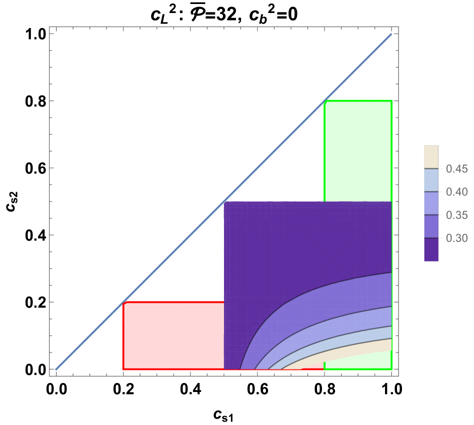
(a) $c_{b}^{2}=-1$

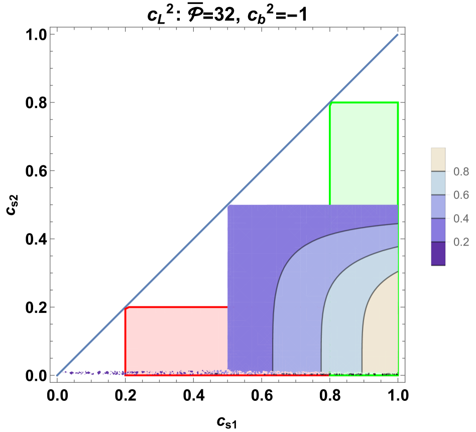
(b) $c_{b}^{2}=0$

Figure 2: $c_{L}^{2}$ as a function of $\left(c_{s1},\,c_{s2},\bar{\cal P}\right)$. The contour plot for $\bar{\cal P}=32$ which maximizes the allowed region. The green curve represents the area covered for smaller values of $\bar{\cal P}$ while the red one shows higher value of $\bar{\cal P}$.

In the stability region, one can choose $\bar{\cal P}$ such that the amplitude of the $\zeta_{n}$ power spectrum is of order $10^{-9}$ as required by observational constraints as shown in Figure 2. We set $\bar{\cal P}$ to a constant, extracting $c_{L}^{2}$ as a function of $\left(c_{s2},\,c_{s1},\,c_{b}^{2}\right)$. When one of the two diagonal sound speeds tends to the longitudinal one, for instance $c_{s1}\to c_{L}$, then $c_{L}$ reduces to its maximal value $\bar{\cal P}^{-\frac{1}{5}}$. The maximal allowed area corresponds to a maximal longitudinal speed $c_{L}=\frac{1}{2}$ and $\bar{\cal P}=32$. Thus, by taking $5<\bar{\cal P}<100$, there is a sufficient large region in the parameters space spanned by $c_{L}$ and $c_{s1},\,c_{s2}$ to get a good agreement with data.

It is useful to study the behavior of the various power spectra when one of the sound speeds is much smaller than the other: $c_{s2}\ll c_{s1}$ with $\bar{\cal P}$ fixed. From our findings (3.38), we get

$$\bar{\cal P}=\frac{(c_{s1}^{2}-c_{L}^{2})}{(c_{b}^{2}-c_{L}^{2})^{2}}\;\left(\frac{c_{b}^{4}}{c_{s1}^{2}}\;\frac{1}{c_{s2}^{5}}+\frac{c_{b}^{2}\;(c_{b}^{2}-2\;c_{s1}^{2})}{c_{s1}^{4}}\;\frac{1}{c_{s2}^{3}}+\frac{(c_{b}^{2}-c_{s1}^{2})^{2}}{c_{s1}^{6}}\;\frac{1}{c_{s2}}\right)+{\cal O}(c_{s2}^{0})\,.$$ (3.43)

This gives, for the different values of $c_{b}$ that we are using, the approximate relations

$$c_{L}^{2}\simeq c_{s1}^{2}+(1-\bar{\cal P}\,c_{s1}^{5})\;\frac{(1+c_{s1}^{2})^{2}}{c_{s1}^{3}}\,c_{s2}^{5}+{\cal O}(c_{s2}^{6})\qquad{\rm for}\qquad c_{b}^{2}=-1\,;$$ (3.44)

$$c_{L}^{2}\simeq c_{s1}^{2}+(1-\bar{\cal P}\,c_{s1}^{5})\,c_{s1}\;c_{s2}+{\cal O}(c_{s2}^{2})\qquad{\rm for}\qquad c_{b}^{2}=0\,.$$ (3.45)

Self consistency requires $c_{s1}^{2}\geq c_{L}^{2}$ that implies $\bar{\cal P}\geq 1/c_{s1}^{5}$; thus if we take $\bar{\cal P}=32$, the two speeds of sound are in the region: $0\leq c_{s2}\ll 1/2\leq c_{s1}\leq 1$. It is precisely the constraint on $\bar{\cal P}$ that introduces a dramatic asymmetry, boosting ${\cal P}_{\scriptscriptstyle{\cal R}_{\pi_{0}}}$. For $c_{b}^{2}=-1$, ${\cal P}_{{\cal R}_{\pi_{0}}}$ is naively enhanced by a factor $1/c_{s2}$

$${\cal P}_{{\cal R}_{\pi_{0}}}={\cal P}_{SF}\;\frac{(1+c_{s1}^{2})^{2}}{c_{s1}^{2}\;(c_{L}^{2}-c_{s1}^{2})\;c_{s2}}+{\cal O}(c_{s2}^{0})\,;$$ (3.46)

however taking into account (3.44), an extra enhancing factor $1/c_{s2}^{6}$ is introduced; namely

$${\cal P}_{{\cal R}_{\pi_{0}}}={\cal P}_{SF}\;\frac{c_{s1}}{\left(c_{s1}{}^{5}\,\bar{\cal P}-1\right)}\,\frac{1}{c_{s2}{}^{6}}+{\cal O}(c_{s2}^{-5})\,.$$ (3.47)

Similarly, for $c_{b}^{2}=0$, an enhancement from $1/c_{s2}$ to $1/c_{s2}^{2}$ is obtained

$${\cal P}_{\scriptscriptstyle{\cal R}_{\pi_{0}}}={\cal P}_{SF}\;\frac{c_{s1}^{2}}{c_{s1}^{2}-c_{L}^{2}}\;\frac{1}{c_{s2}}+{\cal O}(c_{s2})\to{\cal P}_{SF}\;\frac{c_{s1}}{\bar{\cal P}\;c_{s1}^{5}-1}\;\frac{1}{c_{s2}^{2}}+{\cal O}(c_{s2}^{-1})\,.$$ (3.48)

So, the constraint imposed by the observed ${\cal P}_{\zeta_{n}}$ increases the sensitivity to small sound speeds of ${\cal P}_{\scriptscriptstyle{\cal R}_{\pi_{0}}}$ . Thus, at fixed ${\cal P}_{\zeta_{n}}$, the ${\cal P}_{{\cal R}_{\pi_{0}}}$ becomes dominant being proportional to negative powers of $c_{s2}$, see Figure 3.

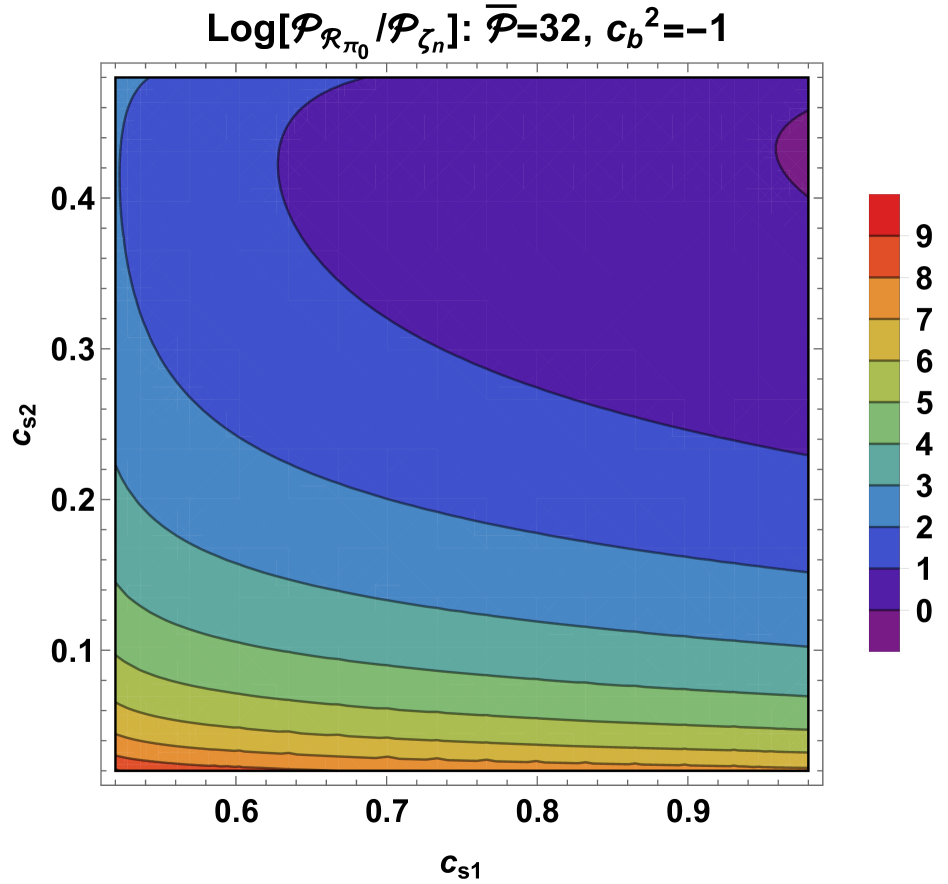
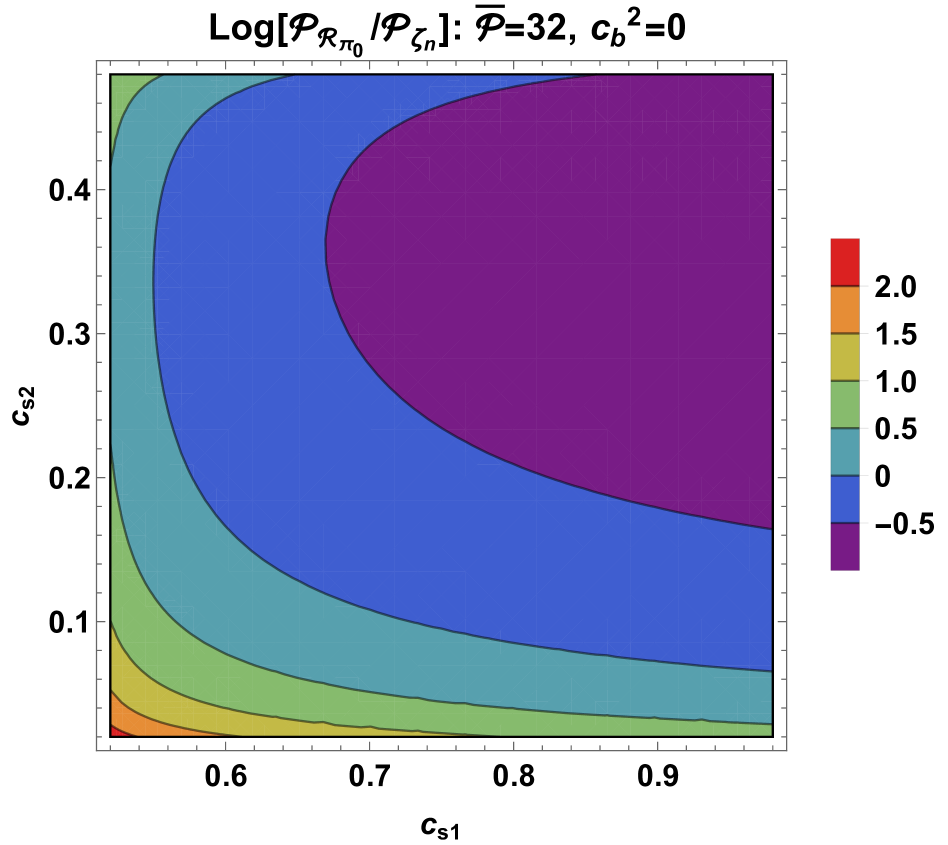
Figure 3: ${\cal P}_{{\cal R}_{\pi_{0}}}/{\cal P}_{\zeta_{n}}$ plot. Note the ${\cal P}_{{\cal R}_{\pi_{0}}}$ enhancement particularly pronounced in the $c_{b}^{2}=-1$ case.

Let us briefly recap the relevant used parameters.
The quadratic Lagrangian contains 5 mass parameters (2, 2.19) or equivalently $c_{0,1,2,3,b}^{2}$ ; it is convenient to replace $c_{4}^{2}$ by $c_{b}^{2}$ in (3.3). On a dS background $c_{s}^{2}=-1$, thus (3.7) fixes $c_{3}^{2}$ to be

$$c_{3}^{2}=\frac{1}{2}+c_{0}^{2}\;c_{b}^{4}+\frac{c_{2}^{2}}{3}\,.$$

In order to generate flat power spectra in a slow-roll regime requires that $-1\leq c_{b}^{2}\leq 0$. Moreover, we were able to find an analytic solution for the modes at any time $t$ only for $c_{b}^{2}=-1$ and $c_{b}^{2}=0$; such values will be considered in the rest of the paper.
It is convenient to trade the three independent parameters $c_{0,1,2}^{2}$ to $c_{L}^{2}$, $c_{s1}^{2}$ and $c_{s2}^{2}$.
While $c_{L}^{2}=-1+\frac{4}{3}\,c_{2}^{2}\,$ can be interpreted as the longitudinal speed typical of Solid Inflation, the other two are the sound speeds corresponding to the two DoFs without any mixing (basically harmonic oscillators) described by (3.28). Finally, by matching the amplitude of the scalar power spectrum to the observed value of $10^{-9}$ one can fix $c_{L}^{2}$ as a function of the remaining two free parameters $c_{s1}^{2}$ and $c_{s2}^{2}$.

Constraints	existence of dS	Analytic modes & $n_{s}\sim 1$	PS amplitude
	$c_{3}^{2}=\frac{1}{2}+c_{0}^{2}\;c_{b}^{4}+\frac{c_{2}^{2}}{3}$	$c_{b}^{2}=-1,\,c_{b}^{2}=0$	${\cal P}_{\scriptscriptstyle\zeta_{n}}(c_{s1}^{2},\,c_{s2}^{2},\,c_{L}^{2})=10^{-9}$
Free parameters	$c_{0,1,2,b}^{2}$	$c_{0,1,2}^{2}$	$c_{s1}^{2},\;c_{s2}^{2}$
$c_{0,1,2,3,4}^{2}$

Table 1: Independent parameters and constraints for supersolids.

Let us note that our results, when comparable, do not agree with the one in [21]. The reason is the missing parameter $c_{b}$ (see footnote 3) and the treatment of the extra scalar degree of freedom in addition to the one present in solid inflation [9].

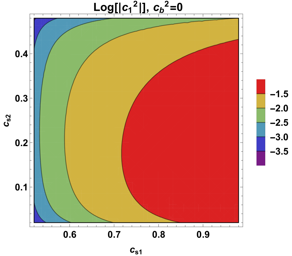
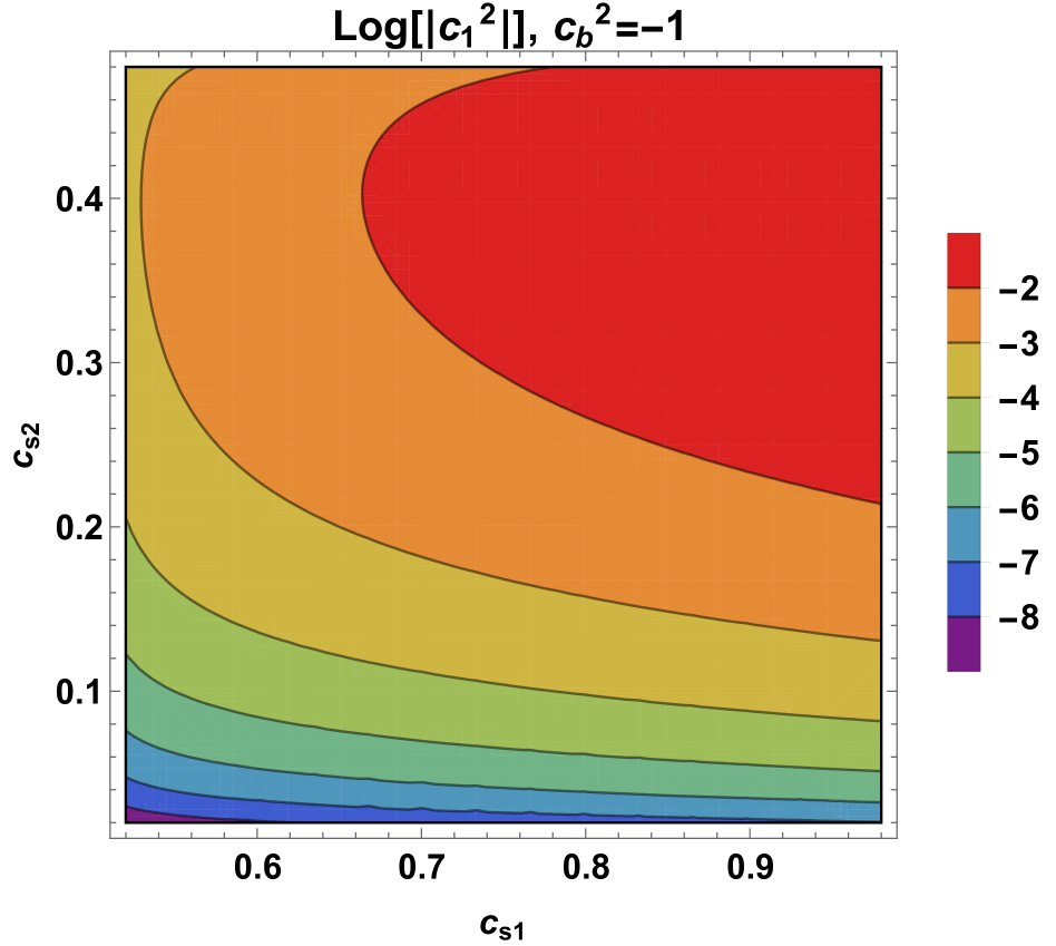
Figure 4: $c_{1}^{2}$ logarithmic contour plot for $c_{b}^{2}=-1$ and $c_{b}^{2}=0$. The parameter $\bar{\cal P}$ is set to $32$.

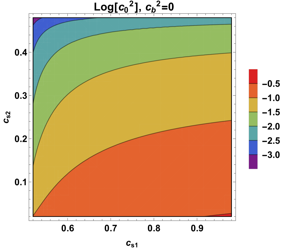
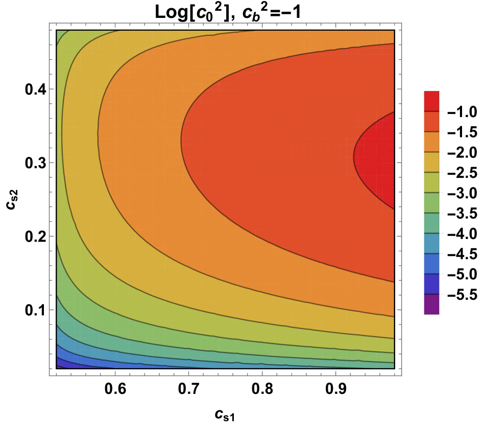
Figure 5: $c_{0}^{2}$ logarithmic contour plot for $c_{b}^{2}=-1$ and $c_{b}^{2}=0$. The parameter $\bar{\cal P}$ is set to $32$.

Taking $c_{s1}$ and $c_{s2}$ as independent parameters, the behavior of $c_{1}$ and $c_{0}$ is important in the study of the amount of isocurvature perturbations and the secondary gravitational waves production. The complete expression is given in Appendix C, we quote here the leading contribution for small $c_{s2}$

$$\begin{split}&c_{1}^{2}=\begin{cases}\left(\frac{1}{c_{s1}}-\bar{\cal P}\,c_{s1}^{4}\right)\,c_{s2}^{5}+O(c_{s2}^{7})\\[5.69046pt] c_{s1}^{3}\frac{(1-\bar{\cal P}\,c_{s1}^{5})}{(1+c_{s1}^{2})^{2}}\,c_{s2}+O(c_{s2})\end{cases}\,\quad c_{0}^{2}=\begin{cases}-\frac{1}{2}\,\left(\frac{1}{c_{s1}}-\bar{\cal P}\,c_{s1}^{4}\right)\,c_{s2}^{3}+O(c_{s2}^{5})&\;\;\;\;c_{b}^{2}=-1\\[5.69046pt] \frac{1}{2}\,c_{s1}^{2}+O(c_{s1})&\;\;\;\;c_{b}^{2}=0\end{cases}\,.\end{split}$$ (3.50)

Note that we have used that ${\cal P}_{\zeta_{n}}=\text{const.}\sim 10^{-9}$ as a fixed constant value. Thus, both $c_{0}$ and $c_{1}$ are suppressed for small $c_{s\,2}$ as shown in figures 4 and 5.

3.2 Slow-roll Corrections at Superhorizon Scales

In this section, we give the slow-roll corrections of the primordial PS, focusing on the two exact solutions obtained for $c_{b}^{2}=-1$ and $c_{b}^{2}=0$. Being the superhorizon behavior determined by the $c_{b}^{2}$ value even at the leading order, the analysis of the large scales $\Pi_{L}$ and $\Pi_{0}$ fields in dS approximation is fundamental in order to get the parameter space where powerspectra are scale-free. By manipulating the system of second order coupled equations (3.31), in the large scale limit $x\ll 1$ , we can get the following two independent fourth-order equations:

$$\Pi_{L}^{(IV)}+\frac{2}{x}\,\Pi_{L}^{{}^{\prime\prime\prime}}-\frac{1}{x^{2}}\left[8+9\,c_{b}^{2}\,(1+c_{b}^{2})\right]\,\Pi_{L}^{{}^{\prime\prime}}+\frac{12}{x^{3}}\,\Pi_{L}^{{}^{\prime}}+\frac{54\,c_{b}^{2}\,(1+c_{b}^{2})}{x^{4}}\Pi_{L}=0\,,$$ (3.51)

$$\Pi_{0}^{(IV)}+\frac{2}{x}\,\Pi_{0}^{{}^{\prime\prime\prime}}-\frac{1}{x^{2}}\left[8+9\,c_{b}^{2}\,(1+c_{b}^{2})\right]\,\Pi_{0}^{{}^{\prime\prime}}+\left[2+9\,c_{b}^{2}\,(1+c_{b}^{2})\right]\,\left[\frac{2}{x^{3}}\,\Pi_{0}^{{}^{\prime}}+\frac{4}{x^{4}}\,\Pi_{0}\right]=0\,.$$

The solutions can be expressed in the following form

$$\Pi_{L}=\frac{1}{\sqrt{k}}\;\left({\cal C}_{L,1}\;x^{-2}+{\cal C}_{L,2}\;x^{3}+{\cal C}_{L,3}\;x^{3\;(1+c_{b}^{2})}+{\cal C}_{L,4}\;x^{-3\;c_{b}^{2}}\right)$$ (3.52)

$$\Pi_{0}=\frac{1}{\sqrt{k}}\;\left({\cal C}_{0,1}\;x^{2+3\;c_{b}^{2}}+{\cal C}_{0,2}\;x^{-1-3\;c_{b}^{2}}+{\cal C}_{0,3}\;x^{-1}+{\cal C}_{0,4}\;x^{4}\right)$$ (3.53)

where the ${\cal C}$ coefficients are unspecified constant at this stage. The ${\cal C}_{L/0,1/2}$ refer to homogeneous solutions while ${\cal C}_{L/0\,3/4}$ to particular solutions of the original system (3.31). Thus, we can understand the effect of $c_{b}^{2}$ on the superhorizon evolution by obtaining particular solutions for $\Pi_{L}$, sourced by $\Pi_{0}$ and vice versa.

	$c_{b}^{2}<-\frac{5}{3}$	$-\frac{5}{3}<c_{b}^{2}<-1$	$-1<c_{b}^{2}<0$	$0<c_{b}^{2}<\frac{2}{3}$	$c_{b}^{2}<\frac{2}{3}$
$\Pi_{L}$	${\cal C}_{L,3}\;\frac{x^{3(1+c_{b}^{2})}}{\sqrt{k}}$	${\cal C}_{L,1}\;\frac{x^{-2}}{\sqrt{k}}$			${\cal C}_{L,4}\;\frac{x^{-3\,c_{b}^{2}}}{\sqrt{k}}$
$\zeta_{n}$	${\cal C}_{L,3}\;\frac{x^{(5+3\,c_{b}^{2})}}{k^{3/2}}$	${\cal C}_{L,1}\;\frac{1}{k^{3/2}}$ Flat PS			${\cal C}_{L,4}\;\frac{x^{(2-3\,c_{b}^{2})}}{k^{3/2}}$
$\Pi_{0}$	${\cal C}_{0,1}\;\frac{x^{(2+3\,c_{b}^{2})}}{\sqrt{k}}$		${\cal C}_{0,3}\;\frac{x^{-1}}{\sqrt{k}}$	${\cal C}_{0,2}\;\frac{x^{-(1+3\,c_{b}^{2})}}{\sqrt{k}}$
${\cal R}_{\pi_{0}}$	${\cal C}_{0,1}\;\frac{x^{3(1+c_{b}^{2})}}{k^{3/2}}$		${\cal C}_{0,3}\;\frac{1}{k^{3/2}}$ Flat PS	${\cal C}_{0,2}\;\frac{x^{-3\,c_{b}^{2}}}{k^{3/2}}$

Table 2: Leading $t$ and $k$ behaviour for $x\to 0$ of $\Pi_{L,0}$ and $\zeta_{n}$, ${\cal R}_{\pi_{0}}$ for different values of $c_{b}^{2}$.

	$c_{b}^{2}=-1$	$-1<c_{b}^{2}<0$	$c_{b}^{2}=0$
$\zeta_{n}$	${\cal C}_{L,1}\;k^{-3/2}$
${\cal R}_{\pi_{0}}$	$({\cal C}_{0,1}+{\cal C}_{0,3})\;k^{-3/2}$	${\cal C}_{0,3}\;k^{-3/2}$	$({\cal C}_{0,3}+{\cal C}_{0,2})\;k^{-3/2}$

Table 3: Inside the region of flat PS $(-1\leq c_{b}^{2}\leq 0)$ we give the late time structure of $\zeta_{n}$ and ${\cal R}_{\pi_{0}}$.

The boundary values for $c_{b}^{2}=-\frac{5}{3},\,-1,\,0,\,\frac{2}{3}$ are shown in Table 3. The relation between $\zeta_{n}$ and ${\cal R}_{\pi_{0}}$ to the canonical fields asymptotically implies the following $k$ and time dependence

$$\begin{split}&\pi_{L}\propto\frac{t^{2}}{k}\;\Pi_{L}\quad\to\quad\zeta_{n}\propto k^{2}\;\pi_{L}\propto k\;t^{2}\;\Pi_{L}\\ &\pi_{0}\propto t^{1+3\;c_{b}^{2}}\;\Pi_{0}\quad\to\quad{\cal R}_{\pi_{0}}\propto t^{-3\;c_{b}^{2}}\;\pi_{0}\propto t\;\Pi_{0}\end{split}$$ (3.54)

Taking into account the various transformations, the almost scale-free PS of $\zeta_{n}$ and ${\cal R}_{\pi_{0}}$ is obtained when the coefficient ${\cal C}_{L,1}$ and ${\cal C}_{0,3}$ dominate. Thus, at the leading order, one realizes that $\zeta_{n}$ is also always almost scale-free in the region $-\frac{5}{3}\leq c_{b}^{2}\leq\frac{2}{3}$, while ${\cal R}_{\pi_{0}}$ selects a smaller region $-1\leq c_{b}^{2}\leq 0$. We will focus on this last region. Recall that ${\cal R}$ and $\zeta$ are simple functions of $(\zeta_{n}\ ,\;{\cal R}_{\pi_{0}})$ and their time derivative, see (3.36, 3.37).

Finally, let us outline the form of the relevant scalar fields at super-horizon scales, obtained by computing the next to leading slow-roll corrections of the canonical normalized fields:

$$\begin{split}\zeta_{n}&={\cal A}_{\zeta_{n}}{}^{(ad)}\,(-H_{i}\,t)^{\alpha^{(ad)}}\,k^{\frac{1}{2}\left[(n_{s}^{(ad)}-1)-3\right]}\,\\ {\cal R}_{\pi_{0}},\,{\cal R},\,\zeta&={\cal A}_{X}^{(ad)}\,(-H_{i}\,t)^{\alpha^{(ad)}}\,k^{\frac{1}{2}\left[(n_{s}^{(ad)}-1)-3\right]}+{\cal A}_{X}^{(en)}\,(-H_{i}\,t)^{\alpha^{(en)}}\,k^{\frac{1}{2}\left[(n_{s}^{(en)}-1)-3\right]}\,;\end{split}$$ (3.55)

the explicit form of the constants ${\cal A}_{a}$ are not relevant here.
Let us explain what superscripts ($ad$) and ($en$) mean. The ($ad$) part of a field stands for its adiabatic part, in the sense that its adiabatic-tilt $n_{s}^{(ad)}$ will not be affected by the presence of the $c_{b}^{2}$ parameter. This parameter is strictly related to the presence of propagating superfluid density per lattice site (i.e. non-barotropic) perturbations. On the contrary, the superscript ($en$) stands for the entropic part of a field, and the related tilt $n_{s}^{(en)}$ will be $c_{b}^{2}$ dependent. A crucial feature is that the behavior of $\zeta_{n}$ on superhorizon scales is determined by a single purely adiabatic power law given in terms of $\alpha^{(ad)}$ and $n_{s}^{(ad)}-1$. As we will show in the next section, in the case of an instantaneous reheating, it is precisely $\zeta_{n}$ that determines the transition to the radiation era, setting the adiabatic part of the initial conditions; moreover, the non-adiabatic part will be determined by the difference $\zeta-\zeta_{n}$. If $c_{b}^{2}$ is far from the interval $[-1,\,0]$, the time dependence from $\alpha^{(en)}$ will overwhelm the homogeneous ${\cal R}_{\pi_{0}}$ solutions, leaving only its particular adiabatic solution. In practice, when we are far enough from the boundary values of $c_{b}^{2}$, also the other fields will be single-tilted; however in this region, the link between super and subhorizon amplitudes needs to be computed numerically.
On the contrary, at the leading order in slow-roll, when $c_{b}^{2}=0,-1$, we get analytical solutions in the form of almost scale-free power laws for all relevant scalars

$${\cal R}_{\pi_{0}},\,{\cal R},\,\zeta\;\to\;\left({\cal A}_{X}^{(ad)}+{\cal A}_{X}^{(en)}\right)\,k^{-\frac{3}{2}}\,.$$ (3.56)

The above form was used in the previous section to compute the leading order amplitudes of the primordial PS for ${\cal R}_{\pi_{0}}$. In practice, when $c_{b}^{2}=0,-1$ we cannot discriminate between the adiabatic and entropic ${\cal R}_{\pi_{0}}$ parts. Such a degeneracy is removed by next to leading slow-roll corrections. In the case of an almost instantaneous reheating, the slow-roll leading order computation of the $\Gamma_{\Lambda\text{CDM}}$, primordial Non-Gaussianities and GWs back-reaction will be sufficient.
For completeness, we give the result of next to leading slow-roll corrections

$$\begin{split}&\qquad\qquad n_{s}^{(ad)}=1+2\,\epsilon_{i}\,c_{L}^{2}-\eta\,,\qquad\alpha^{(ad)}=\frac{4}{3}\,c_{T}^{2}\,\epsilon,\\ &\begin{cases}&n_{s}^{(en)}=7+6\,c_{b}^{2}\,(1+\epsilon_{i})+\eta\,,\;\;\alpha^{(en)}=3+3\,c_{b}^{2}\,(1+\epsilon)+\epsilon+\eta\,,\qquad\text{dominant if}\;c_{b}^{2}\approx-1\,,\\ &n_{s}^{(en)}=1-6\,c_{b}^{2}\,(1+\epsilon_{i})-\eta\,,\;\;\alpha^{(en)}=-6\,c_{b}^{2}\,(1+\epsilon)-\eta\,,\qquad\text{dominant if}\;c_{b}^{2}\approx 0\,.\end{cases}\end{split}$$ (3.57)

The ($ad$) tilt is formally the same as the one found in [9], being obtained by solving the same superhorizon equations of motion. However, starting from a supersolid, the solid inflation limit does not exist: the extra degree of freedom cannot be smoothly switched off. In principle, two ($en$) tilts are present in the other fields and exists only on the edges of the region.
Let us sketch the main steps to get the above slow-roll corrections on superhorizon scales:

1. Trade the system of coupled equations for $\left(\zeta_{n},\,{\cal R}_{\pi_{0}}\right)$ for an equivalent but simpler to analyze involving $\left({\cal R},\,\delta\sigma\right)$;

2. Find the canonical fields $({\cal R}_{c},\,\delta\sigma_{c})$ and find the leading superhorizon behaviour at the leading order in slow-roll as done for $\left(\Pi_{L},\,\Pi_{0}\right)$. Define the ($ad$) part of ${\cal R}$ as its “homogeneous” (e.g. $c_{b}$ independent) component (coherent with the fact that $\zeta_{n}$ is a purely “adiabatic” field) and the ($en$) part of ${\cal R}$ as the $\delta\sigma$-sourced solutions.

3. Compute the ${\cal R}$ and $\delta\sigma$ slow-roll corrections on superhorizon scales.

4. Degeneracy breaking:

   • for $c_{b}^{2}=-1$, $\delta\sigma$ is a dominant decoupled (en) source on superhorizon scales, which means that

     $$\delta\sigma=\delta\sigma^{(ad)}+\delta\sigma^{(en)}\equiv\delta\sigma^{(en)}\qquad\Rightarrow\delta\sigma^{(ad)}(\zeta_{n},\,{\cal R}_{\pi_{0}})=0\,;$$ (3.58)

   • When $c_{b}^{2}=0$, ${\cal R}$ is a dominant decoupled ($ad$) source on superhorizon scales, which means that

     $${\cal R}={\cal R}^{(ad)}+{\cal R}^{(en)}\equiv{\cal R}^{(ad)}\qquad\Rightarrow{\cal R}^{(en)}(\zeta_{n},\,{\cal R}_{\pi_{0}})=0\,.$$ (3.59)

Following the above steps, one arrives at eq. (3.55) and, in addition, the degeneracy is resolved by

$$\begin{split}&c_{b}^{2}=-1\,,\;\;\;\zeta_{n}^{(ad)}+\frac{1}{3}\,\frac{c_{0}^{2}}{c_{b}^{2}}\,\frac{1}{\bar{\varphi}^{\prime}}\left(\frac{\bar{\varphi}^{\prime}}{{\cal H}}\,{\cal R}_{\pi_{0}}^{(ad)}\right)^{\prime}=0\,.\\ &c_{b}^{2}=0\,,\;\;\;{\cal R}_{\pi_{0}}^{(en)}\to 0\,.\end{split}$$ (3.60)

A degeneracy in the amplitude persists for $c_{b}^{2}=-1$ . In that case, by using eq. (LABEL:split), we get

$${\cal R}_{\pi_{0}}^{(ad)}=\frac{3\,c_{b}^{2}}{c_{0}^{2}\,(2-3\,c_{b}^{2})}\,\zeta_{n}\,,\qquad{\cal R}_{\pi_{0}}^{(en)}={\cal R}_{\pi_{0}}-{\cal R}_{\pi_{0}}^{(ad)}\,.$$ (3.61)

Furthermore, being ${\cal R}_{\pi_{0}}^{(ad)}\sim c_{0}^{-2}\,\zeta_{n}$, for small $c_{s\,2}$ one has

$${\cal R}_{\pi_{0}}^{(ad)}\ll{\cal R}_{\pi_{0}}^{(en)}\approx{\cal R}_{\pi_{0}}\,.$$ (3.62)

As will be shown in the next section, $\zeta_{n}$ provides the seed for adiabatic perturbations at the beginning of radiation domination; as a result CMB data [27] imply that its spectral index $n_{s}^{(ad)}$ has to be red tilted. Thus, when $c_{b}^{2}=0$, ${\cal R}_{\pi_{0}}$ will be red-tilted too. However, when $c_{b}^{2}=-1$, ${\cal R}_{\pi_{0}}$ has two components with different spectral indices, one is still $n_{s}^{(ad)}$ and the second is $n_{s}^{(en)}$. For small deviation from $c_{b}^{2}=-1$, one can set

$$c_{b}^{2}=-1+\delta_{b}\,,$$ (3.63)

and the deviation from $n_{s}^{(en)}=1$ turns out to be

$$n_{s}^{(en)}\approx 1+6\,(\delta_{b}-\epsilon)+\eta\,;$$ (3.64)

which can be blue-tilted. The consequences for the secondary production of gravitational waves is rather interesting and studied in section 6.

4 Reheating

Once the seed of primordial perturbations is produced, it is important to study how the Universe reheats and gets to the radiation domination era. In single clock inflation, the hypothesis of the Weinberg theorem are satisfied [1] and the inflationary predictions are largely independent of reheating, however this is not the case when more then one field is present, as for solid and supersolid inflation, where neither ${\cal R}$ nor $\zeta$ are conserved on super horizon scales and moreover ${\cal R}\neq\zeta$. As a consequence of the presence of $\varphi^{0}$, the pressure perturbation is not proportional to $\delta\rho$

$$\delta p=c_{s}^{2}\,\delta p+\Gamma\,,\qquad\Gamma=\frac{\phi^{\prime}\left(c_{b}^{2}-c_{s}^{2}\right)}{a^{4}}\delta\sigma\,;$$ (4.1)

thus the $\Gamma$ signals the presence of non-adiabatic perturbations. Dealing with more than one component like in $\Lambda$CDM, non-adiabaticity can also be present when the relative energy density perturbations of two components are different: $\delta_{i}\neq\delta_{j}$. The total non-adiabaticity $\Gamma_{\text{tot}}$ contains both the intrinsic contribution for each component of the form (4.1) and the “relative” part $\Gamma_{\text{rel}}$ that takes into account that $\delta_{i}$ is not simply caused by the “universal” temperature perturbation. In the case of $\Lambda$CDM with a barotropic equation of state for all the components only $\Gamma_{\text{rel}}$ is present and then $\Gamma_{\Lambda\text{CDM}}\equiv\Gamma_{\text{rel}}$; at superhorizon scales one gets

$$\zeta={\cal R}=\zeta_{0}+\int_{a_{in}}^{a}\frac{\Gamma_{\Lambda\text{CDM}}}{(1+w)\,\rho\,\tilde{a}}\,d\tilde{a}\,;$$ (4.2)

where $\zeta_{0}$ is the adiabatic constant contribution. For a recent discussion see [7].
A pragmatic approach is to assume that reheating takes place instantaneously on a time-like hypersurface given in terms of a 4-scalar $q$ as $q=$constant, or expanding at the linear order in perturbation theory

$$\bar{q}+\delta q=\text{constant}\,.$$ (4.3)

A generic physical quantity ${\cal F}$ will be denoted by the subscript ${\cal F}_{-}$ when evaluated at the end of inflation, and with ${\cal F}_{+}$ when evaluated at the end of reheating. Thus, the change of ${\cal F}$ across $q$ will be simply written as

$$[{\cal F}]_{\pm}={\cal F}_{+}-{\cal F}_{-}\,,$$ (4.4)

and the transition will be dictated by the Israel junction conditions [28]. By generalizing the results in [29], in the general gauge (B.1), such conditions read at the linear level

$$\left[\zeta_{q}\right]_{\pm}\equiv\left[-\Phi+{\cal H}\frac{\delta q}{\bar{q}^{\prime}}\right]_{\pm}=0\,;$$ (4.5)

$$\left[\left(1-\frac{{\cal H}^{\prime}}{{\cal H}^{2}}\right)\left({\cal R}-\zeta_{q}\right)\right]_{\pm}=0\,;$$ (4.6)

$$\left[\Phi_{gi}\right]_{\pm}\equiv\left[\Phi+{\cal H}\left(F-B^{\prime}\right)\right]_{\pm}=0\,.$$ (4.7)

At the background level, the junction conditions imply that both $a$ and ${\cal H}$ are continuous on $q$. The quantity $\zeta_{q}$ represents the gauge invariant curvature perturbation of a constant $q$-hypersurface, and thus it is continuous across $q$. From the transformation properties (B.4), one can easily show that the junction conditions are gauge invariant.
As a reasonable assumption, we will take $q$ to be the particle number density $n$. Intuitively, in the approximation of an instantaneous reheating, the rate for any channel for the decay of inflatons into a particle A becomes very large and the decay itself is democratic, in the sense if $n_{A}$ is the number density of the particle A and $n$ is the total number density, then

$$\frac{\delta n_{A}}{\bar{n}_{A}}\to\frac{r_{A}\,\delta n}{r_{A}\,\bar{n}}\equiv\frac{\delta n}{\bar{n}}\,;$$ (4.8)

from the above relation and the particle number conservation $\bar{n}^{\prime}+3\,{\cal H}\,\bar{n}=0$ we have that

$$\left[\frac{\delta n}{\bar{n}^{\prime}}\right]_{\pm}=0\,.$$ (4.9)

In the flat gauge, where $\Phi=0$, such a condition is precisely (4.5) with $q=n$

$$\left[\zeta_{n}\right]_{\pm}=0\,,$$ (4.10)

When the field $\varphi^{0}$ is absent, namely $M_{0}=M_{1}=0$ (solid inflation limit), one is back to the standard case where reheating takes place at a constant energy density $\rho$ hypersurface like in [9, 20]. The continuity of $\zeta_{n}$ can also be shown following the same lines of [20] by a generalization of the procedure given in [30]. By using the definition of $\zeta_{n}$ and $\delta\sigma$ we have that

$$\zeta=\zeta_{n}-\frac{\delta\sigma\;\phi^{\prime}}{18\,M_{\text{Pl}}^{2}\,a^{2}\,(w+1)\mathcal{H}^{2}}\equiv\zeta_{n}+\frac{\Gamma_{\text{eff}}}{3\,\rho\,(1+w)\,c_{s}^{2}}\,.$$ (4.11)

By integrating by parts the relation which gives ${\cal R}^{\prime}$ and by using the time-time component of the Einstein equations, see [20], one gets

$$\left[{\cal R}\right]_{\pm}=\left[\frac{1}{3}\frac{k^{2}\Phi}{{\cal H}^{2}\epsilon}+\frac{\Gamma_{\text{eff}}}{3\,\rho\,(1+w)\,c_{s}^{2}}\right]_{\pm}\,;$$ (4.12)

where the effective intrinsic entropic perturbation $\Gamma_{\text{eff}}$ before/after reheating is defined as follows:

$$\text{Inflation:}\;\;\;\Gamma_{\text{eff}}=-\frac{\bar{\varphi}^{\prime}}{a^{4}}\,c_{s}^{2}\,\delta\sigma\,,\qquad\text{Radiation:}\;\;\;\Gamma_{\text{eff}}=\Gamma_{\Lambda\text{CDM}}\,.$$ (4.13)

Then (4.12), is equivalent to

$$\left[\zeta-\frac{\Gamma_{\text{eff}}}{3\,\rho\,(1+w)\,c_{s}^{2}}\right]_{\pm}=\left[\zeta_{n}\right]_{\pm}=0\,,$$ (4.14)

demonstrating our intuition (4.10).
By using (3.6) and (4.10) the second junction condition (4.6) reads

$${\cal R}_{+}=\zeta_{n}+\frac{\epsilon}{\epsilon_{+}}\left({\cal R}_{-}-\zeta_{n}\right)\,,\qquad\qquad\qquad\epsilon_{+}=\left(1-\frac{{\cal H}^{\prime}}{{\cal H}^{2}}\right)_{|\text{radiation}}\approx 2\,,$$ (4.15)

Let us consider the most important case where, after the Universe reheats, a vanilla $\Lambda$CDM radiation dominated era is reached, for which at superhorizon scales

$${\cal R}_{+}=\zeta_{+}\,.$$ (4.16)

From the above relation and by using (4.15), the jump of $\zeta$ across the reheating hypersurface is

$$\left[\zeta\right]_{\pm}={\cal R}_{+}-\zeta_{-}=\left(\zeta_{n}-\zeta_{-}\right)+\frac{\epsilon}{\epsilon_{+}}\left({\cal R}_{-}-\zeta_{n}\right)\,;$$ (4.17)

where, being $\zeta_{n}$ continuous, $\zeta_{n}{}_{+}=\zeta_{n}{}_{-}$ and has been denoted simply by $\zeta_{n}$.
Finally, one can calculate the total amount of non-adiabaticity $\Gamma_{\Lambda\text{CDM}}$ present at the beginning of the radiation era. Indeed, by comparison with (4.14)

$$\left[\frac{\Gamma_{\text{eff}}}{3\,\rho\,(1+w)\,c_{s}^{2}}\right]_{\pm}=\frac{\Gamma_{\Lambda\text{CDM}}}{3\,\rho\,(1+w)\,c_{s}^{2}}_{|\text{Rad}}-\;\frac{\Gamma_{\text{eff}}}{3\,\rho\,(1+w)\,c_{s}^{2}}_{|\text{Infl}}=\left[\zeta\right]_{\pm}$$ (4.18)

The jump of $\zeta$ is given by (4.17), thus

$$\Gamma_{\Lambda\text{CDM}}=\frac{4}{3}\,\rho_{\text{Rad}}\left[\frac{\Gamma_{\text{eff}}}{3\,\rho\,(1+w)\,c_{s}^{2}}_{|\text{Infl}}+\left(\zeta_{n}-\zeta_{-}\right)+\frac{\epsilon}{\epsilon_{+}}\left({\cal R}_{-}-\zeta_{n}\right)\right]\\ =\frac{2}{3}\,\rho_{\text{Rad}}\,\epsilon\,\left({\cal R}_{-}-\zeta_{n}\right)\,;$$

finally, taking into account that the above relation refers to superhorizon scales, from the results of Appendix B and C we arrive at

$$\Gamma_{\Lambda\text{CDM}} = \frac{2}{3}\,\rho_{\text{Rad}}\,\epsilon\,\left[{\cal H}(1+c_{1}^{2})\pi_{L}^{\prime}-c_{1}^{2}{\cal R}_{\pi_{0}}-\zeta_{n}\right]$$ (4.19)

$$\approx -\frac{2}{3}\,\rho_{\text{Rad}}\,\epsilon\,\sum_{j=1}^{2}\left[\zeta_{n}^{(j)}\left(1+c_{s\,j}^{2}(1+c_{1}^{2})\right)+c_{1}^{2}\,{\cal R}_{\pi_{0}}^{(j)}\right]\,.$$

Note that the contribution to the transmitted $\Gamma$ stays small for small $c_{s2}$. Indeed, from eqs. (3.50), we get that

$$\epsilon\,c_{1}^{2}\,{\cal R}_{\pi_{0}}^{(2)}\propto\begin{cases}\epsilon\,c_{s2}^{2}&c_{b}^{2}=-1\\ \epsilon\,c_{s2}^{\frac{1}{2}}&c_{b}^{2}=0\end{cases}\,.$$ (4.20)

There is still a point to address. Take a generic field $X$ that satisfies a second order evolution equation with two independent solutions: one $X_{cg}$, growing or constant with scale factor $a$, and a second one $X_{d}$ decreasing with $a$. Clearly, the physically relevant solution is $X_{cg}$; however, even if the junction conditions prescribe that $\left[X\right]=0$, the constant/growing mode alone can be discontinuous. A classic example is given by the gauge invariant Bardeen potential $\Phi_{gi}$, which according to (4.7) is continuous in the transition at constant $\rho$ with a sudden change of equation of state in $\Lambda$CDM; however, from the continuity of $\zeta$ constant mode, one gets

$$\Phi_{gi\,+}\mid_{\text{constant mode}}=\Phi_{gi\,-}\mid_{\text{constant mode}}\,\frac{(1+w_{+})}{(1+w_{-})}\frac{(5+3\,w_{-})}{(5+3\,w_{+})}\,.$$ (4.21)

Things are different in our non-adiabatic case. A clear understanding of the behavior of $\Phi_{gi}$ constant mode is crucial to predict the correct back reaction of tensor modes during radiation domination. Indeed, the validity of (4.21) crucially implies that the $\Phi_{gi}$ gains a factor $\epsilon^{-1}$ entering radiation domination. For simplicity, in the rest of this section we will work in Newtonian gauge, where $\Phi_{gi}$ coincides with $\Phi$. For each classic scalar field, it is convenient to distinguish among constant, decaying (absent during inflation) and entropic (particular solution proportional to the non-adiabatic source term proportional to $\Gamma$) modes. Once the decaying modes are under control, in principle, a reshuffling of constant and entropic modes in the junction conditions is still possible. Focusing on the entropic source $\Gamma_{\Lambda\text{CDM}}$ relative to $\Lambda$CDM where dark energy is just a cosmological constant; neglecting baryons during radiation domination, we have two fluids: dark matter and photons as discussed in [7] and $\Gamma_{\Lambda\text{CDM}}$ assumes the form

$$\Gamma_{\Lambda\text{CDM}}=\frac{8\,H_{0}^{2}\,M_{pl}^{2}\,\Omega_{m}\,\Omega_{r}}{a^{3}\,\left(4\,\Omega_{r}+3\,a\,\Omega_{m}\right)}\,s_{0}(k)\,;$$ (4.22)

with $s_{0}(k)$ a scale dependent constant that is determined by using (4.19) at $t_{+}=-t_{-}$ . At superhorizon scales, the non-adiabatic contribution to $\zeta$ reads

$$\zeta|_{en}=s_{0}(k)\,\frac{a\,\Omega_{m}}{3\,a\,\Omega_{m}+4\,\Omega_{r}}\,,$$ (4.23)

while the contribution to $\zeta_{n}$ is

$$\zeta_{n}|_{en}=\zeta|_{en}-\frac{\Gamma_{\Lambda\text{CDM}}}{3\,(\rho+p)\,c_{s}^{2}}\equiv 0\,.$$ (4.24)

Thus, during inflation $\zeta_{n}$ acts always as a source term for ${\cal\zeta}$, ${\cal R}$ and $\delta\sigma$ when $-1\leq c_{b}^{2}\leq 0$. The same exactly happens during the radiation domination where any entropic contribution to $\zeta_{n}$ is compensated by an opposite contribution from $\zeta$ or ${\cal R}$ leading to

$$\left[\zeta_{n}\right]|_{\text{constant modes}}\equiv 0\,.$$ (4.25)

Following [30], expressing $\zeta_{n}$ in terms of the Bardeen potentials in the Newtonian gauge, we get

$$\zeta_{n}=-\Phi-\frac{2(\Phi^{\prime}+{\cal H}\,\Psi)}{3\,{\cal H}\,(1+w)}-\frac{2\,k^{2}\,\Phi}{9\,(1+w)\,{\cal H}^{2}}-\frac{\Gamma_{\text{eff}}}{3\,\rho\,(1+w)\,c_{s}^{2}}\,,$$ (4.26)

eq. (4.21) is non longer valid. Imposing that

$$\zeta_{n}|_{en}=0\,,$$ (4.27)

we get

$$\Phi|_{en}+\frac{2(\Phi^{\prime}+{\cal H}\,\Phi)}{3\,{\cal H}\,(1+w)}|_{en}+\frac{\Gamma_{\Lambda\text{CDM}}}{3\,\rho\,(1+w)\,c_{s}^{2}}=0\,.$$ (4.28)

Considering the early stages of radiation domination, where dark energy is negligible, we have

$$\Phi_{\text{rad}}\to-\frac{s_{0}(k)}{5\,a^{3}}\,\left[a^{3}-2\,a^{2}\,a_{e}+8\,a\,a_{e}^{2}+16\,a_{e}^{3}\right]\,,$$ (4.29)

where $a_{eq}=\frac{\Omega_{r}}{\Omega_{m}}$ is the scale factor at the matter radiation equality and we normalized the today’s scale factor as $a_{0}=1$. The same results could have been obtained by directly solving the $\Phi$ equation of motion or equivalently by expressing $\zeta$ in terms of $\Phi$ and $\Phi^{\prime}$ and enforcing that $\zeta_{n}$ is not affected by non-adiabatic perturbations. Thus, eliminating $\Gamma_{\text{eff}}$ from (4.26), we can extract the constant $\Phi$ mode during the radiation phase

$$\Phi|_{\text{constant mode}}=-\frac{3\,(1+w)}{5+3\,w}\,\zeta_{n}\,,\qquad w\to\frac{1}{3}\,,$$ (4.30)

which is similar to the standard result with $\zeta$ replaced by $\zeta_{n}$. The result (4.30) is not compatible with eq. (4.21) that would imply the transmission of the ${\cal R}_{\pi_{0}}$ in the constant mode of $\Phi$. Thus, $\Phi$ gets an enhancement of order $\epsilon^{-1}$ when the Universe transits into the radiation era, without a further enhancement due to the presence of ${\cal R}_{\pi_{0}}$ during inflation. Summarizing, in the case of an instantaneous reheating, $\zeta_{n}$ determines initial conditions at superhorizon scales for the standard evolution for the $\Lambda$CDM scenario with small deviations from a perfectly adiabatic spectrum of primordial perturbations.

5 Primordial Non Gaussianity: a preview

Primordial Non-Gaussianity (NG) is an essential tool to distinguish among different models of inflation. Single field inflation with its characteristic symmetry breaking pattern gives a small amount NG in the scalar and tensor sector, with the scalar part peaked in the local shape. A complete analysis of NG in supersolid inflation will be given in a companion paper [16], here we will outline some of the results needed to study the secondary production of GWs. Given the presence of two scalars and tensor fields, the full cubic action for a supersolid is quite complicated. Cubic terms can involve three scalars (SSS), one scalar and two tensors (TTS), two scalars and one tensor (TSS) and three tensors (TTT); each contribution to the cubic Lagrangian ${\cal L}^{(3)}$ in Fourier representation has the following general structure

$${\cal L}^{(3)}\sim\omega\,M_{\text{pl}}^{2}\,H^{2}\,a^{m}\,D_{k\,k^{\prime}\,k^{\prime\prime}}\,\xi_{1,\,k}\,\xi_{2,\,k^{\prime}}\,\xi_{3,\,k^{\prime\prime}}\,,$$ (5.1)

where $\omega$ is a constant that sets the overall size of the vertex and $m$ determines its time evolution in terms of the scale factor $a$; finally $D$ is a dimensionless function of the momenta and is determined by the structure of spatial derivatives acting on the fields entering the vertex denoted by $\xi_{i,k}$ which can be any combination of $\zeta_{n}$, $H^{-1}\,\zeta_{n}^{\prime}$, ${\cal R}_{\pi_{0}}$, $H^{-1}\,{\cal R}_{\pi_{0}}^{\prime}$, and $h^{s}$; $h^{s}$ is the spin two tensor field (indices are omitted). In general, one can show that

$$f_{\text{NL}}\sim\frac{\omega}{\epsilon}\,.$$ (5.2)

The value of $\omega$ is determined by the relative size of the derivatives of the Lagrangian density $U$ of the scalar sector with respect to the rotational invariant independent operators. In [9] it was assumed the presence of a partial cancellation among the derivatives of $U$ such that, even in slow-roll, $\omega\sim 1$. Such extreme choice maximizes the deviation from single field inflation, pumping up local NG to $f_{\text{NL}}\sim\epsilon^{-1}$ which is in trouble with recent Plank constraints [31]. Here we take a more conservative approach, considering that each derivative of $U$ is of order $\epsilon$ in slow-roll expansion, leading to

$$\omega=\alpha\,\epsilon\,,$$ (5.3)

with $\alpha$ an order one quantity. As a result, we get that $f_{\text{NL}}\sim O(\epsilon^{0})$ and, in addition, the cutoff of the effective field theory describing a supersolid is higher. Compared with NG in solid inflation, the presence of an additional scalar introduces non-adiabatic perturbations controlled by the parameter $c_{b}^{2}$. This parameter has an important effect on any 3-point function involving ${\cal R}_{\pi_{0}}$ and, as we have seen, on the PS of ${\cal R}_{\pi_{0}}$ itself as discussed in section 3.1.
In particular, when $c_{b}^{2}\to 0$, we can show that the local $f_{\text{NL}}$ tends to be unacceptably big and strongly scale-dependent, unless some rather unnatural tuning is made. As a result, when primordial NG is considered, the best choice is to take $c_{b}^{2}\approx-1$. As it will be shown in the next section, in this case, supersolid inflation features a rather exciting boost of the secondary gravitation waves production during inflation thanks to the cubic mixed TSS that is promising for future experiments.

6 Gravitational Waves

Given the current experimental upper bound on the tensor to scalar ratio $r\leq 0.5$, it is important to discriminate among different inflationary models by telling how close to the limit the prediction for $r$ can be. Indeed, in the next few years, we will be able to probe the region $\in\left(10^{-1}\,\div\,10^{-2}\right)$. Our analysis is similar to the one in [32], where secondary gravitational waves generated by a spectator scalar field was studied. However, in that specific case, taking into account the related secondary scalar PS, considerably reduces the ratio $r$ [33]. On the contrary, in our supersolid model of inflation, the dominant cubic scalar vertex (SSS) is essentially unrelated to the dominant tensor-scalar-scalar (TSS) cubic one. That gives us room to effectively enhance $r$ to get close to its experimental upper limit with only the secondary tensor production. That feature singles out supersolid from single field inflationary models where the dominant GW production is not very sensitive to NG and gravitational waves back-reaction is much smaller than the one generated during the radiation phase as it was observed originally in [34, 35, 36] and later extended in [37, 38].

Spin two tensor perturbations are defined by

$$g_{ij}=a^{2}\,\left(\delta_{ij}+h_{ij}\right)\,,\qquad\qquad\delta_{ij}h_{ij}=\partial_{j}h_{ij}=0\,;$$ (6.1)

where $h_{ij}$ is the transverse and traceless part of the metric tensor. During Inflation, the corresponding quadratic/cubic Lagrangian can be written as

$$L_{T}=M_{pl}^{2}\,a^{2}\left[\frac{1}{2}\left(h_{ij}{}^{\prime}\,h_{ij}{}^{\prime}-(M_{2}\,a^{2}-\partial^{2})\,h_{ij}h_{ij}\right)+h_{ij}\,{\cal S}_{ij}\right]\,,$$ (6.2)

where $S_{ij}$ is a transverse-traceless quadratic-source term. The evolution equation for GWs is

$$h_{ij}^{\prime\prime}+2\;{\cal H}\;h_{ij}^{\prime}-\Delta\;h_{ij}={\cal S}_{ij}\,.$$ (6.3)

where we neglect the mass $M_{2}$ being proportional to $\epsilon$, see (2.19). The leading contribution to ${\cal S}_{ij}$ comes from the cubic interaction terms containing one spin two field $h_{ij}$ and two scalars. There is a “universal” contribution from cubic terms in the Einstein-Hilbert Lagrangian and a graviton scalar interactions in the “matter” sector; namely ${\cal S}_{ij}={\cal S}^{(EH)}_{ij}+{\cal S}^{(\text{Matter})}_{ij}$. The leading structure of the EH interactions comes from derivatives of scalar perturbations and has the following structure

$$\begin{split}\,{\cal S}^{(EH)}_{ij}\propto\;\partial_{i}\Phi_{gi}\,\partial_{j}\Phi_{gi}\,.\end{split}$$ (6.4)

The matter contribution ${\cal S}^{(\text{Matter})}_{ij}$ changes effectively during the universe evolution . In our case, during the inflationary period (where Matter = Inflaton), among all the possible TSS vertices, the dominant one is given by the following cubic lagrangian (see the structure in (5.1))

$${\cal L}^{(3)}_{TSS}=-\epsilon\,\alpha\,a^{2}\;M_{pl}^{2}\;k^{\prime i}\;k^{\prime\prime j}\;h_{ij}(k)\;{\cal R}_{\pi_{0}}(k^{\prime})\;{\cal R}_{\pi_{0}}(k^{\prime\prime})\qquad\to\quad{\cal S}^{(\text{Infl})}_{ij}=\epsilon\,\alpha\,a^{2}\,\partial_{i}{\cal R}_{\pi_{0}}\,\partial_{j}{\cal R}_{\pi_{0}}\,,$$ (6.6)

with $\alpha$ a constant given by

$$\alpha=2\,\left(c_{2\,w}^{2}-c_{1}^{2}\right)\,;$$ (6.7)

where

$$\begin{split}c_{2}^{2}\equiv c_{2\,\tau}^{2}+&c_{2\,w}^{2};\qquad c_{2\,\tau}^{2}=-\frac{a^{2}}{9\,{\cal H}^{2}\,\epsilon}\left(U_{\tau_{y}}+U_{\tau_{z}}\right)\,;\qquad c_{2\,w}^{2}=-\frac{a^{2}}{9\,{\cal H}^{2}\,\epsilon}\left(U_{w_{y}}+U_{w_{z}}\right)\,;\end{split}$$ (6.8)

with $c_{2\,w}^{2}$ the part of $M_{2}$  proportional to the derivatives of $U$ with respect to the operators $\{w_{i}\}$.
The analysis of the role of the operators $w_{i}$ is interesting. At the zero and first order in the perturbation theory they are degenerate with the operators $\{\tau_{i}\}$, so are sensitive only to the solid structure of the medium. It is only at second order that the $\{w_{i}\}$ start to discriminate a solid from a supersolid. From the structure of the $\{w_{i}\}$, we see that the $\varphi^{0}$ scalar field, related to the superfluid part, is intrinsically coupled to the $\varphi^{a}$ fields, describing the solid side. Thus, while the presence of the operators $\{w_{i}\}$ is immaterial at the linear level, it plays an important role for non-Gaussianity. If the operators $\{w_{i}\}$ are absent, automatically $c_{2\,w}=0$ and $\alpha=-2\,c_{1}^{2}$. However, from (3.50), in this case

$$\alpha\sim c_{s2}^{5}\ll 1$$

and TSS vertex is negligible. The only constraint on $c_{2\,w}^{2}$ comes from stability: $c_{L}^{2}>2\,c_{0}^{2}\,c_{b}^{4}$ and $c_{s\,2}^{2}<c_{L}^{2}<c_{s1}^{2}$.
Given the presence of ${\cal R}_{\pi_{0}}$, the size of the source is very sensitive to the value of $c_{s2}$ (typically $\propto c_{s2}^{-3}$). In our specific case, during inflation, we get that the Einstein Hilbert term is always suppressed ${\cal S}^{(\text{Infl})}\gg{\cal S}^{(EH)}$, while during the radiation phase nothing more than what is described in [37, 38] happens; the only difference is that the Bardeen potential is proportional to $\zeta_{n}$ instead of $\zeta$, see (4.30). The tensor PS has two contributions: one (primary PS) ${\cal P}_{h}^{(1)}$ from the quantum fluctuations during the dS period and calculated with the homogeneous quadratic action of $h_{ij}$, and another classical contribution (secondary PS) ${\cal P}_{h}^{(2)}$ coming from the interactions of $h_{ij}$ with the other scalar fluctuations. This last term can be calculated by finding the particular solution of (6.3) proportional to ${\cal S}^{(Matter)}$. The computation of the primary tensor PS is standard; denoting with $H_{i}$ the Hubble parameter during the dS phase, in the case $c_{b}^{2}=-1$ we have

$${\cal P}_{h}^{(1)}=\frac{H_{i}^{2}}{8\,M_{pl}^{2}\,\pi^{2}}\,(-t\,k)^{\frac{8}{3}\,c_{2}^{2}\,\epsilon}\,k^{2\,c_{L}^{2}\,\epsilon}\,\simeq\epsilon\;\frac{{\cal P}_{\zeta_{n}}}{\bar{\cal P}}.$$ (6.9)

Remember that $\zeta_{n}$ fluctuations represent the primordial seed for scalar perturbations during the radiation phase. The particular solution of (6.3) can be obtained by using the Green function ($g_{k}(t,\,t^{\prime})$) method

$$\begin{split}&h(t,\,k)=\int_{-\infty}^{t}g_{k}(t,\,t^{\prime})\,{\cal S}_{k}(t^{\prime})\,dt^{\prime}\,,\qquad{\cal S}=\varepsilon_{ij}^{(s)\,*}\,{\cal S}_{ij}\,,\\[5.69046pt] &\;\;\partial_{t}^{2}\,g_{k}(t,\,t^{\prime})+2\,{\cal H}\;\partial_{t}\,g_{k}(t,\,t^{\prime})+k^{2}\,g_{k}(t,\,t^{\prime})=\delta(t-t^{\prime})\,.\end{split}$$ (6.10)

The above solution can be used to extract the PS ${\cal P}_{h}^{(2)}$ for the secondary production of GWs as

$$(2\,\pi)^{3}\,P_{h}^{(2)}(k\,t)\,\delta(\textbf{k}-\textbf{p})\equiv\int_{-\infty}^{t}\int_{-\infty}^{t}\,dt^{\prime}\,dt^{\prime\prime}\,g_{k}(t,\,t^{\prime})\,g_{p}(t,\,t^{\prime\prime})\,\langle S_{k}(t^{\prime})\,S_{p}(t^{\prime\prime})\rangle\,,$$ (6.11)

where $\langle S_{k}(t^{\prime})\,S_{p}(t^{\prime})\rangle$ represents a Gaussian 4-point scalar correlator. During the inflationary period, the above correlator is proportional to $\langle{\cal R}_{\pi_{0}}^{4}\rangle$; in the limit of a small $c_{s2}$ one gets the following estimate for the secondary scale-invariant PS

$${\cal P}_{h}^{(2)}\approx\alpha^{2}\,\epsilon^{2}\,\frac{2\,\pi^{2}}{c_{s2}}\,{\cal P}_{{\cal R}_{\pi_{0}}}^{2}\,=\alpha^{2}\,\epsilon^{2}\,\gamma^{2}\;\frac{2\,\pi^{2}}{c_{s2}^{13}\;\bar{\cal P}^{2}}\,{\cal P}_{\zeta_{n}}^{2}\,\,,$$ (6.12)

where we have defined $\gamma$ such that

$${\cal P}_{{\cal R}_{\pi_{0}}}=\gamma\;\frac{{\cal P}_{\zeta_{n}}}{c_{s2}^{6}\;\bar{\cal P}}\,.$$ (6.13)

The final expression for the total tensor PS is given by

$${\cal P}_{h}={\cal P}_{h}^{(1)}+{\cal P}_{h}^{(2)}={\cal P}_{\zeta_{n}}\;\frac{\epsilon}{\bar{\cal P}}\left(1+\alpha^{2}\,\epsilon\,\gamma^{2}\;\frac{2\,\pi^{2}}{c_{s2}^{13}\;\bar{\cal P}}\,{\cal P}_{\zeta_{n}}\right)\,.$$ (6.14)

The presence of the coupling constant (6.6) which controls the TSS vertex gives rise to the question of whether the cubic scalar interactions can give sizeable contributions to the scalar PS. The SSS dominant interaction Lagrangian for the scalar one loop corrections to ${\cal P}_{\zeta_{n}}$ has the following structure (5.1)

$${\cal L}^{(3)}_{SSS}=-\epsilon\,a^{2}\,M_{\text{pl}}^{2}\;\left[\beta_{2}\;k^{\prime i}\,k^{\prime\prime i}\;+\beta_{1}\;\frac{k^{i}\,k^{j}\;k^{\prime i}\,k^{\prime\prime j}}{k^{2}}\right]\,\,\zeta_{n}(k)\;{\cal R}_{\pi_{0}}(k^{\prime})\;{\cal R}_{\pi_{0}}(k^{\prime\prime}),$$ (6.15)

and when $c_{b}^{2}\approx-1$

$$\beta_{1}=12\,c_{2\,w}^{2}\,,\qquad\beta_{2}=-\frac{1}{2}\left\{3\,\frac{\sigma}{M_{\text{pl}}^{2}\,H^{2}\,\epsilon}-4\,\left[c_{2\,w}^{2}+3\,\left(c_{0}^{2}\,c_{b}^{2}+\frac{U_{by}}{8\,H^{2}\,\epsilon}\right)\right]\right\}\,.$$ (6.16)

As usual, $U_{by}$ and $\sigma$ will be taken to be of order $\epsilon$ to get $\beta_{i}$ order one, as discussed in the previous section. Furthermore, while $\beta_{1}$ vanishes in the absence of $w$-operators, $\beta_{2}$ is generically different from zero. For generic $\beta_{i}\sim 1$, the computation of the non-linear correction to the scalar PS is complicated. A reasonable estimate is given by

$$\begin{split}&{\cal P}_{\zeta_{n}}^{(2)}\propto\epsilon^{2}\,\beta_{i}^{2}\,\frac{2\,\pi^{2}}{c_{s_{2}}}\,{\cal P}_{{\cal R}_{\pi_{0}}}^{2}=\epsilon^{2}\,\beta_{i}^{2}\,\gamma^{2}\frac{2\,\pi^{2}}{c_{s_{2}}^{13}\;\bar{\cal P}^{2}}\,{\cal P}_{\zeta_{n}}^{2}\,,\end{split}$$ (6.17)

with the total scalar PS given by ${\cal P}_{\zeta_{n}}+{\cal P}_{\zeta_{n}}^{(2)}$. The possibility to have a regime where the secondary tensor production is dominant while the secondary scalar contribution is negligible, namely

$$\frac{{\cal P}_{h}^{(2)}}{{\cal P}_{h}^{(1)}}\gg 1\,,\qquad\frac{{\cal P}_{\zeta_{n}}^{(2)}}{{\cal P}_{\zeta_{n}}}\ll 1\,,$$ (6.18)

gives

$$\epsilon\ll\frac{\alpha^{2}}{\beta^{2}}\,\bar{\cal P},\qquad\frac{2\,\pi^{2}\,\gamma^{2}\,{\cal P}_{\zeta_{n}}}{\bar{\cal P}}\,\frac{\beta^{2}\,\epsilon^{2}}{\bar{\cal P}}\ll c_{s2}^{13}\ll\frac{2\,\pi^{2}\,\gamma^{2}\,{\cal P}_{\zeta_{n}}}{\bar{\cal P}}\,\alpha^{2}\,\epsilon\,.$$ (6.19)

Taking $\gamma\sim 1$, ${\cal P}_{\zeta_{n}}=10^{-9}$ and $\bar{\cal P}=32$ we get

$$0.15\;\left(\beta^{2}\,\epsilon^{2}\right)^{1/13}\ll c_{s2}\ll 0.2\;\left(\alpha^{2}\,\epsilon\right)^{1/13}\,.$$ (6.20)

Relation (6.20) is valid whether or not the operator $w_{i}$ are present. However, when $c_{2\,w}^{2}$ is zero, the inequality

$$\beta^{2}\epsilon^{2}<\alpha^{2}\,\epsilon\sim{c_{s2}}^{10}\,\epsilon\,,$$ (6.21)

is valid only if $\epsilon$ is very small, and then is much more tuned. The presence of the parameter $c_{2\,w}^{2}$ makes the gravitational waves secondary production dominant for a suitable region of the parameters space, even if the ${\cal R}_{\pi_{0}}$ is not efficiently transmitted in the scalar sector after inflation. Even the case where the secondary scalar and tensor production are both relevant is interesting. A rough estimate gives

$$r=\frac{{\cal P}_{h}^{(2)}}{{\cal P}_{\zeta_{n}}^{(2)}}=\frac{\beta_{i}^{2}}{\alpha^{2}}\,,$$ (6.22)

which is very sensitive to the detail of the non-linear structure of the theory.
Let us mention that, even if a cubic coupling between tensors and transverse vectors of the schematic form $h_{ij}(\pi_{i}^{\prime}\pi_{j}^{\prime}+\partial\pi_{i}\partial\pi_{j})$ exists, we do not expect an enhancement similar to the one found due to the scalars. The transverse vector sector is very similar to solid inflation, and in the limit of small $c_{s\,2}$

$$\langle\pi_{i}\,\pi_{i}\rangle\sim O(c_{s\,2}{}^{0})\,,$$

with $\pi_{i}$ defined by the linear theory. Thus, the secondary production of GWs from the vector sector is much smaller than the one from the scalar sector which is of order ${\cal P}_{{\cal R}_{\pi_{0}}}{}^{2}$.
All the above expressions are given at the leading order in a slow-roll expansion and the PS are scale-free, modulo small slow-roll corrections.
Finally, let us estimate the tilt of secondary GWs production. The next to leading corrections to the primordial tensor PS can be obtained by simply substituting ${\cal P}_{{\cal R}_{\pi_{0}}}$ in eq. (6.12) with the complete expression $k^{3}\,|{\cal R}_{\pi_{0}}|^{2}/(2\,\pi^{2})$. In the $c_{b}^{2}=-1$ case, we have three contributions with three different tilts (see eq. (3.55)): $n_{s}^{(ad)}$, $n_{s}^{(en)}$, and

$$n_{s}^{(ad-en)}=\frac{n_{s}^{(ad)}+n_{s}^{(en)}}{2}\,.$$ (6.23)

As we argued, there is the possibility to get a blue-tilted index for $n_{s}^{(en)}$ tilt, and being $n_{s}^{(ad)}$ red-tilted, the ($en$) index term will be the dominant one for scales much smaller than the CMB ones ,

$${\cal P}_{{\cal R}_{\pi_{0}}}\to{\cal P}_{{\cal R}_{\pi_{0}}}^{(en)}\,(-H\,t)^{6\,\delta_{b}-5\,\epsilon+\eta}\,k^{n_{s}^{(en)}-1}\,.$$ (6.24)

Thus, eq. (6.12) reduces to

$${\cal P}_{h}^{(2)}\approx\alpha^{2}\,\epsilon_{i}^{2}\,\frac{2\,\pi^{2}}{c_{s2}}\,{\cal P}_{{\cal R}_{\pi_{0}}}^{(en)}{}^{2}\,(-H\,t)^{12\,\delta_{b}-10\,\epsilon}\;k^{2(n_{s}^{(en)}-1)}\,,$$ (6.25)

then

$$n_{T}=2\,n_{s}^{(en)}-1\equiv 1+12\,(\delta_{b}-\epsilon_{i})+2\,\eta\,,$$ (6.26)

which is blue tilte when

$$\delta_{b}>\epsilon_{i}-\frac{\eta}{6}\,.$$ (6.27)

The presence of a blue $n_{T}$ parameter will be an interesting tool to test inflationary models in future high sensitivity experiments of Gravitational waves detection[39]. Indeed, for modes that re-enter the horizon during radiation domination, the GWs energy density spectrum[40, 41] goes as

$$\Omega_{GW}\propto k^{n_{T}-1}\,,$$ (6.28)

if $n_{T}-1>0$, it could grow up to the frequencies $f=c\,k/2\pi$ in the milli-Hertz band, where we expect the maximum of LISA sensitivity[42, 43].

7 Conclusion

An extreme synthesis of the production of the seeds for cosmological perturbations in supersolid inflation is given in Table 4 where the magnitude and the fate of the leading order power spectra of scalar and tensorial perturbations are shown.

$\quad\underbrace{{\cal P}^{(1)}_{en}\sim\left(\frac{{\cal P}^{(1)}_{ad}}{c_{s2}^{6}}\right)\quad\gg\quad{\cal P}^{(1)}_{ad/en}\sim\left(\frac{{\cal P}^{(1)}_{ad}}{c_{s2}^{3}}\right)}_{\rm Dissipated\,during\,the\,reheating}\quad\gg\quad\underbrace{{\cal P}^{(1)}_{ad}\sim 10^{-9}\quad\gg\quad{\cal P}^{(1)}_{h}\sim\epsilon\;{\cal P}^{(1)}_{ad}}_{\rm transmitted\,during\,the\,reheating}\qquad$

Table 4: Relations among power spectra (leading order) and their fate in a instantaneous reheating, in the limit $c_{s2}\ll 1$.
$ad=$ adiabatic (${\cal P}^{(1)}_{ad}={\cal P}^{(1)}_{\zeta_{n}}$) and $en=$ entropic (${\cal P}^{(1)}_{en}={\cal P}^{(1)}_{{\cal R}_{\pi_{0}}}$)

.

Adiabatic perturbations are related to the solid part of the medium ($\zeta_{n}\propto\pi_{L}\propto\varphi^{i}$). The presence of large entropic perturbations, related to its superfluid component (${\cal R}_{\pi_{0}}\propto\pi_{0}\propto\varphi^{0}$), potentially can enhance the PS of the other fields by next to leading corrections.
The secondary production is generically suppressed for inflaton-like fields , tensor perturbations play the role of spectator fields (with a PS proportional to $H^{2}_{i}/(M_{pl}^{2})$) and the interaction with entropic scalar perturbations enhances considerably their secondary PS. Indeed, the following scenario is possible We have systematically explored the physical consequences of the breaking of the full set of diffeomorphism of general relativity down to $ISO(3)$. The breaking pattern is triggered by the background configuration of four scalar fields and, in order to allow dS spacetime as a solution, we have considered an additional set of internal symmetries comprising $SO(3)$ internal rotations and four shift symmetries. The four scalars $\varphi^{A}$ can be interpreted as the coordinates of a supersolid embedded in spacetime and the corresponding effective Lagrangian we have studied is the most general one consistent with the given symmetries at the leading order in a derivative expansion. As a comparison, in the effective description of single clock inflation [26] the residual symmetry comprises three dimensional diffeomorphism with one scalar and two tensor propagating modes, while in our supersolid inflation, we have two scalars, two transverse vectors and two tensors. Interestingly, as a benefit of the supersolid interpretation, the scalar field fluctuations can be interpreted as phonons modes and non-adiabatic perturbations. Given the symmetry breaking pattern and the number of propagating modes, the difference with single clock inflation are significant both at the linear and non-linear levels. At the linear level, the symmetry breaking pattern gives rise to a peculiar kinetic mixing between the two scalars that makes the quantization and the computation of the linear power spectra non-trivial. A similar (but different) mixing is found in chromo-natural inflationary models [23, 24, 25], non-thermal production of gravitinos [22], multi-field inflation [23] and in effective theories of inflation[21]. Our analysis and results differ from the previous ones: we do not use perturbations theory to resolve the kinetic mixing but rely on Hamiltonian analysis and a set of canonical transformations to reduced the dynamical system to two uncoupled harmonic oscillators in the limit of large momentum $k$. As a consequence, cross-correlations in the scalar power spectra are unavoidable. The presence of the scalar $\varphi^{0}$ associated with the superfluid component introduces the important parameter $c_{b}^{2}$ for the superhorizon evolution of the scalars. The hypothesis of the Weinberg theorem are explicitly violated. Indeed, we get both the presence of the anisotropic stress which is not negligible in the $k\to 0$ limit, and perturbations are non-adiabatic in general. Thus, neither the comoving curvature perturbation ${\cal R}$ nor the curvature perturbation $\zeta$ are conserved, moreover they differ on superhorizon scales, though their superhorizon evolution is only due to small slow-roll corrections. In the range $c_{b}^{2}\in[-1,\,0]$, all the relevant scalar power spectra are scale-free, modulo small slow-roll corrections, in agreement with experimental constraints. Because of the presence of two scalar propagating degrees of freedom, there is no smooth limit that leads to solid inflation [9] and thus the predictions at the level of linear power spectra are rather different. The system of coupled second order differential equations for the linear evolution of the two independent scalar perturbations are complicated enough due to the non-trivial kinetic mixing to elude an analytical solution for a generic time $t$ unless $c_{b}^{2}=0,\,-1$. Luckily enough, these boundary values for $c_{b}^{2}$ are such that the relevant power spectra are almost scale-free. Among the various scalar perturbations, we select the power spectra of the curvature perturbation $\zeta_{n}$ of the constant particle number $n$ hypersurface and and curvature perturbation ${\cal R}_{\pi_{0}}$ of the constant $\varphi^{0}$ hypersurface and the relative cross correlations, studying in detail their properties as a function of $c_{b}^{2}$ and the speed of sounds of the two independent diagonal scalar modes. In the instantaneous reheating approximation, by extending the analysis in [29], we analyze how the seed of primordial perturbations are transmitted to the standard hot radiation dominated era of $\Lambda$CDM. Besides the standard adiabatic component, a small isocurvature part can be written as a linear combination of $\zeta_{n}$ and ${\cal R}_{\pi_{0}}$ evaluated at the end of inflation. Also the prediction for primordial non-Gaussianity is rather interesting; we leave a detailed account for a companion paper, focusing on the secondary production of gravitational waves during inflation. The structure of the tensor-scalar-scalar cubic vertex is such that it is possible to enhance the secondary production, saturating the experimental bound, still keeping the scalar bispectrum within the limits set by Planck. Finally, the spectral index of GWs PS can be blue-tilted, enhancing the chance of a direct detection of the primordial stochastic background.
In conclusion, supersolid inflation is an interesting alternative to single clock inflation to explore different symmetry breaking patterns with a clear experimental signature.

Appendix A Parameters ${\boldsymbol{M_{\alpha}}}$

The parameters $\left\{M_{\alpha}\,;\alpha=0,1,3,4\right\}$ entering in the quadratic action (2) are defined by the following derivatives of the Lagrangian density around the background

$$\bar{g}_{\mu\nu}=a(t)^{2}\,\eta_{\mu\nu}\,,\qquad\bar{\varphi}^{0}=\bar{\varphi}(t)\,,\qquad\bar{\varphi}^{i}=x^{i}\,\qquad i=1,2,3\,.$$ (A.1)

$$M_{0}=\frac{\bar{\varphi}^{\prime}{}^{2}\left(U_{\chi\chi}+2\,U_{y\chi}+U_{yy}\right)}{2a^{2}}\,,\qquad M_{1}=-\frac{\bar{\varphi}^{\prime}{}\,U_{\chi}}{a}\,,\qquad M_{2}=-\frac{4}{9}\left(U_{w_{Y}}+U_{w_{Z}}+U_{\tau_{Y}}+U_{\tau_{Z}}\right)\,,$$

$$M_{3}=\frac{M_{2}}{3}+\frac{1}{2}\,a^{-6}\,U_{bb}\,,\qquad M_{4}=\frac{\bar{\varphi}^{\prime}\left[U_{b\chi}+U_{by}-a^{3}\left(U_{\chi}+U_{y}\right)\right]}{2a^{4}}\,;$$ (A.2)

where all the derivatives are evaluated on the background values of the operators by which $U$ depends on. The Minkowski background corresponds to $\bar{\varphi}^{\prime}=a=1$.

Appendix B Gauge Invariant Operators and Perturbations

Being the background $SO(3)$ invariant, cosmological perturbations can be decomposed in a scalar, vector, and tensor sector. In a generic gauge, scalar perturbations can be written as

$$\varphi^{0}=\bar{\varphi}^{\prime}+\pi_{0}\,,\qquad\varphi^{i}=x^{i}+\partial^{i}\pi_{L}+\pi_{T}^{i}\,,$$ (B.1)

$$g_{00}=-a^{2}\,(1-2\,\Psi)\,,\qquad g_{0i}=a^{2}\,\partial_{i}F\,,\qquad g_{ij}=a^{2}\,\left[(1+2\,\Phi)\,\delta_{ij}+2\,\partial_{ij}B\right]\,.$$ (B.2)

Consider an infinitesimal coordinates transformation; in the scalar sector we have that

$$x^{\mu}\to\tilde{x}^{\mu}=x^{\mu}+\epsilon^{\mu}\,,\qquad\epsilon^{\mu}=(\epsilon^{0},\,\partial^{i}\beta)\,.$$ (B.3)

The scalar parts of metric and the perturbation of $\varphi^{A}$ transform according with 

$$\begin{split}&\Delta_{\text{gauge}}\Psi=\epsilon^{0}{}^{\prime}+{\cal H}\,\epsilon^{0}\,,\qquad\Delta_{\text{gauge}}F=\epsilon^{0}-\beta^{\prime}\,,\qquad\Delta_{\text{gauge}}\Phi=-{\cal H}\,\epsilon^{0}\,,\\ &\Delta_{\text{gauge}}B=-\beta\,,\;\;\qquad\qquad\Delta_{\text{gauge}}\pi_{0}=-\bar{\varphi}^{\prime}\,\epsilon^{0}\,,\qquad\Delta_{\text{gauge}}\pi_{L}=-\beta\,.\end{split}$$ (B.4)

From the above transformation properties, one can construct the following gauge invariant perturbations

$$\pi_{L,\,gi}=\pi_{L}-B\,,\qquad\qquad\pi_{0,\,gi}=\pi_{0}-\frac{\bar{\varphi}^{\prime}}{{\cal H}}\Phi\,;$$ (B.5)

and the corresponding curvature perturbations

$$\zeta_{n}=\frac{k^{2}}{3}\pi_{L,\,gi}=-\Phi+\frac{{\cal H}}{\bar{n}^{\prime}}\,\delta n\,,\qquad\qquad{\cal R}_{\pi_{0}}=\frac{{\cal H}}{\bar{\varphi}^{\prime}}\pi_{0,\,gi}=-\Phi+\frac{{\cal H}}{\bar{\varphi}^{\prime}}\,\pi_{0}\,.$$ (B.6)

Together with

$$\begin{split}&\zeta=\Phi+{\cal H}\frac{\delta\rho}{\bar{\rho}^{\prime}}\,;\\ &{\cal R}=\Phi+{\cal H}\,v,\end{split}$$ (B.7)

$\zeta_{n}$ and ${\cal R}_{\pi_{0}}$ represent the fundamental gauge invariant scalars. While $\zeta_{n}$ represents the curvature of constant number density hypersurfaces, ${\cal R}_{\pi_{0}}$ can be identified as the curvature perturbation orthogonal to the velocity of the superfluid component in the supersolid, see (2.15); whose spatial part, at the linear level is given by

$$\nu^{i}=-\frac{1}{\bar{\varphi}^{\prime}}\,\partial_{i}\pi_{0}\,.$$ (B.8)

From (2.14), we have

$$\delta\sigma=\frac{2\,a^{4}\,M_{\text{Pl}}^{2}\,M_{0}}{\bar{\varphi}^{\prime}}\left[\Psi+3\,c_{b}^{2}\,\Phi+\frac{\pi_{0}^{\prime}}{\bar{\varphi}^{\prime}}+c_{b}^{2}\,k^{2}\pi_{L,\,gi}\right]\,,$$ (B.9)

and it is gauge invariant; taking the time derivative we arrive at

$$\delta\sigma^{\prime}=\frac{k^{2}\,a^{4}\,M_{\text{Pl}}^{2}\,M_{1}}{\bar{\varphi}^{\prime}}\left[\frac{\pi_{0}}{\bar{\varphi}^{\prime}}-\pi_{L,\,gi}{}^{\prime}+(F-B^{\prime})\right]\,.$$ (B.10)

Adiabatic media, solids for instance, are characterized by $u^{\mu}\partial_{\mu}\sigma=0$ at the non-perturbative level. This is the case when the Lagrangian $U$ does not depend on $\chi$ in [20]. In particular, this implies that at the linearized level $M_{1}=0$, in perfect agreement with (B.10) which for such a class of media gives $\delta\sigma^{\prime}=0$. The linearized EMT can be written as the perturbed EMT for a perfect fluid plus an anisotropic stress contribution

$$T_{\nu}^{\mu}=(\bar{p}+\bar{\rho}+\delta p+\delta\rho)\;\bar{\mathfrak{U}}^{\mu}\;\bar{\mathfrak{U}}_{\nu}+(\bar{p}+\bar{\rho})\;(\delta\mathfrak{U}^{\mu}\;\bar{\mathfrak{U}}_{\nu}+\bar{\mathfrak{U}}^{\mu}\;\delta\mathfrak{U}_{\nu})+(\bar{p}+\delta p)\;\delta^{\mu}_{\nu}+\Pi^{\mu}_{\nu}\,,$$ (B.11)

where $\bar{\mathfrak{U}}_{\mu}=(-a,\vec{0})$ is the background 4-velocity, $\delta\rho,\;\delta p$ are the perturbations of energy density and pressure. The anisotropic stress is turned on by the presence of $\tau_{Y}$, $\tau_{Z}$. $w_{Y}$ and $w_{Z}$. In the scalar sector, the velocity $\delta\mathfrak{U}^{\mu}$ and the anisotropic stress perturbations $\Pi^{\mu}_{\nu}$ can be written in terms of two extra scalars $v$ and $\Xi$ , in addition to $\delta\rho$

$$\begin{split}&\delta\mathfrak{U}_{\mu}=(a\;\Psi,\;a\,\partial_{i}v),\qquad\Pi^{\mu}_{\nu}\equiv\;(3\;\partial^{2}\,\delta^{\mu}_{i}\;\delta^{i}_{\nu}-\delta^{\mu}_{i}\,\partial^{i}\,\delta_{\nu}^{j}\partial_{j})\;\Xi\,,\\ &\Xi\equiv-2\,a^{2}\,M_{2}\,\pi_{L\,gi}=2\left[\Phi-\Psi+2{\cal H}\,(F-B^{\prime})+(F-B^{\prime})^{\prime}\right]\,,\end{split}$$ (B.12)

with

$$\begin{split}&\delta\rho=-\bar{\rho}(1+w)(3\Phi+k^{2}\pi_{L,\,gi})+a^{-4}\,\bar{\varphi}^{\prime}\,\delta\,\sigma\,,\\ &v=-\pi_{L,\,gi}^{\prime}+\frac{M_{1}\,a^{2}}{6\,{\cal H}^{2}\,(1+w)}\left[\frac{\pi_{0}}{\bar{\varphi}^{\prime}}-\pi_{L,\,gi}{}^{\prime}+(F-B^{\prime})\right]+(F-B^{\prime})\,.\end{split}$$ (B.13)

Using this parameterization, ${\cal R}$, $\zeta$ and $\sigma$ can be easily written in terms of $\pi_{L}$, $\pi_{0}$ and their derivative w.r.t. conformal time. Namely, with the suffix $gi$ understood, we have

$$\begin{split}{\cal R}=&\epsilon\,(1+c_{1}^{2})\,\left(1-2\,c_{0}^{2}\,c_{b}^{2}\right)\,{\cal H}^{2}\,\pi_{L}+c_{1}^{2}\,{\cal H}\,\left[-1+3\,\epsilon\,(1+c_{1}^{2})\,\frac{{\cal H}^{2}}{k^{2}}\right]\,\frac{\pi_{0}}{\bar{\varphi}^{\prime}}\\ &+(1+c_{1}^{2})\,\left[1-3\,\epsilon\,(1+c_{1}^{2})\,\frac{{\cal H}^{2}}{k^{2}}\right]\,{\cal H}\,\pi_{L}^{\prime}-2\,\epsilon\,(1+c_{1}^{2})\,\frac{{\cal H}^{2}}{k^{2}}\,\frac{\pi_{0}^{\prime}}{\bar{\varphi}^{\prime}}\,,\end{split}$$ (B.14)

$$\begin{split}\zeta=&\frac{k^{2}}{3}\,(1-2\,c_{0}^{2}\,c_{b}^{2})\,\pi_{L}-\frac{2}{3}\,\epsilon\,c_{0}^{2}\,c_{1}^{2}\,{\cal H}\,\frac{\pi_{0}}{\bar{\varphi}^{\prime}}\\ &+\frac{2}{3}\,\epsilon\,c_{0}^{2}\,{\cal H}\,(1+c_{1}^{2})\,\pi_{L}^{\prime}-\frac{2}{3}\,c_{0}^{2}\,\frac{\pi_{0}^{\prime}}{\bar{\varphi}^{\prime}}\,,\end{split}$$ (B.15)

$$\delta\sigma=-2\,a^{4}\,\bar{\rho}\,\bar{\varphi}^{\prime-1}\,\left(\zeta-\zeta_{n}\right)\,\epsilon\,.$$ (B.16)

The above expressions are valid at the linear order in the slow-roll parameters.

Appendix C Canonical Transformation

In the UV (large $k$) the Lagrangian (3.22) becomes

$$L_{2}^{\text{(UV})}=\frac{1}{2}\Pi^{\prime}{}^{t}\Pi^{\prime}-\Pi^{t}\,{\cal D}^{\text{UV}}\,\Pi^{\prime}-\frac{1}{2}\Pi^{t}\,{\cal M}^{\text{UV}}\,\Pi\;$$ (C.1)

with

$${\cal D}\to{\cal D}^{\text{UV}}\equiv{\cal D}\,,\qquad{\cal M}\to{\cal M}^{\text{UV}}=\begin{pmatrix}k^{2}\,\lambda_{L}{}^{2}&0\\ 0&k^{2}\,\lambda_{0}{}^{2}\end{pmatrix}$$ (C.2)

The first step is to find the Hamiltonian density corresponding to (3.22), which reads

$${\cal H}=\frac{1}{2}\,P^{t}\,P-P^{t}\,{\cal D}\,\Pi+\frac{1}{2}\,\Pi^{t}\,\left({\cal M}-{{\cal D}^{\text{UV}}}^{2}\right)\,\Pi\,,$$ (C.3)

where $P$ is the conjugate momentum of $\Pi$

$$P=\Pi^{\prime}+{{\cal D}^{\text{UV}}}\,\Pi\,.$$ (C.4)

The decoupled system can be obtained by applying a canonical transformation of the form:

$$\begin{split}&\Pi=A\,\tilde{\Pi}+B\,\tilde{P}\,,\\ &P=J\,\tilde{P}+C\,\tilde{\Pi}\,.\\ \end{split}$$ (C.5)

Using (2.19), imposing that the transformation is canonical with the new ${\cal D}_{c}$ vanishing, the four matrices $A$, $B$, $J$ and $C$ can be taken of the following form

$$A=\begin{pmatrix}1&0\\ 0&1\par\end{pmatrix}\,,\;\;\;J=\frac{1}{2}\left(1+\frac{\Delta\lambda}{\Delta}\right)\begin{pmatrix}1&0\\ 0&1\end{pmatrix}\,,\;\;\;B=-2\,\frac{d}{k\,\Delta}\begin{pmatrix}0&1\\ 1&0\end{pmatrix}\,,\;\;\;C=-k\,\frac{\Delta\lambda-\Delta}{4\,d}\begin{pmatrix}0&1\\ 1&0\end{pmatrix}\,,$$ (C.6)

where $\Delta\lambda$ and $\Delta$ are given by

$$\Delta\lambda=\lambda_{0}^{2}-\lambda_{L}^{2}\,,\qquad\Delta=\frac{\left(4\,c_{0}^{4}\,c_{L}^{4}+c_{1}^{4}\,\left[1+8\,c_{0}^{2}(c_{L}^{2}-c_{b}^{2})\right]+4\,c_{0}^{2}\,c_{1}^{2}\,\left[c_{L}^{2}+4\,c_{0}^{2}\,c_{b}^{2}\,(c_{L}^{2}-c_{b}^{2})\right]\right)^{\frac{1}{2}}}{2\,c_{0}^{2}\,(1+c_{1}^{2})}\,.$$ (C.7)

The transformed Hamiltonian reads

$${\cal H}_{\text{new}}=\frac{1}{2}\,\tilde{P}^{t}\,{\cal K}_{\text{new}}\,\tilde{P}+\frac{1}{2}\,\tilde{\Pi}^{t}\,{\cal M}_{\text{new}}\,\tilde{\Pi}\,,$$ (C.8)

with

$${\cal K}_{\text{new}}=A+B\,(C+{\cal D})\equiv\begin{pmatrix}{\cal K}_{1\text{new}}&0\\ 0&{\cal K}_{2\text{new}}\end{pmatrix}\,,\qquad{\cal M}_{\text{new}}=-B^{-1}\,(C-{\cal D})\equiv\begin{pmatrix}{\cal M}_{1}&0\\ 0&{\cal M}_{2}\end{pmatrix}\,;$$ (C.9)

both ${\cal K}_{\text{new}}$ and ${\cal M}_{\text{new}}$ are diagonal and thus, for fixed $k$, (C.8) describes two uncoupled harmonic oscillators with frequencies $k^{2}\,c_{s1}^{2}$ and $k^{2}\,c_{s2}^{2}$, where

$$c_{s1}^{2}=\frac{{\cal M}_{1}\,{\cal K}_{1\text{new}}}{k^{2}}=d^{2}+\lambda_{L}^{2}+\frac{\Delta\lambda}{2}+\frac{\Delta}{2}\,,\qquad c_{s2}^{2}=\frac{{\cal M}_{2}\,{\cal K}_{2\text{new}}}{k^{2}}=2\,d^{2}+\lambda_{L}^{2}+\frac{\Delta\lambda}{2}-\frac{\Delta}{2}\,.$$ (C.10)

Quantization of (C.8) is straightforward: the Bunch-Davies vacuum is the state $|0\rangle$ of the Fock space corresponding to the following field operators

$$\tilde{\Pi}=\begin{pmatrix}\tilde{\Pi}_{1}\\ \tilde{\Pi}_{2}\end{pmatrix}=\begin{pmatrix}A_{k}^{(1)}\,a_{k}{}^{(1)}\,e^{-i\,k\,c_{s1}\,t}+A_{k}^{(1)\,*}\,a_{k}{}^{(1)\,\dagger}\,e^{i\,k\,c_{s1}\,t}\\ A_{k}^{(2)}\,a_{k}{}^{(2)}\,e^{-i\,k\,c_{s2}\,t}+A_{k}^{(2)\,*}\,a_{k}{}^{(2)\,\dagger}\,e^{i\,k\,c_{s2}\,t}\end{pmatrix}\,,\qquad A_{k}^{(n)}=k^{-\frac{1}{2}}\,\left(\frac{{\cal K}_{n}}{c_{sn}}\right)^{\frac{1}{2}}$$ (C.11)

with $a_{k}{}^{(1/2)\,\dagger}$ and $a_{k}{}^{(1/2)}$ standard creation and annihilation operators. The fields satisfies the following canonical commutation relations

$$\left[\tilde{\Pi}_{m}(t,\textbf{x})\,,\;\tilde{\Pi}_{n}^{\prime}(t,\textbf{y})\right]=i\,{\cal K}_{m}\,\delta^{(3)}\left(\textbf{x}-\textbf{y}\right)\,\delta_{mn}\,,\qquad m,n=1,2\,.$$ (C.12)

By using (LABEL:can_tr), one can express $\Pi_{L}$ and $\Pi_{0}$ in terms of the creation and annihilation operators

$$\Pi_{L}=\sum_{j=1}^{2}C_{L}^{(j)}\,a_{k}^{(j)}\,e^{-i\,k\,c_{s\,j}\,t}+C_{L}^{(j)\,*}\,a_{k}^{(j)\,\dagger}\,e^{i\,k\,c_{s\,j}\,t},,$$ (C.13)

$$\Pi_{0}=\sum_{j=1}^{2}C_{0}^{(j)}\,a_{k}^{(j)}\,e^{-i\,k\,c_{s\,j}\,t}+C_{0}^{(j)\,*}\,a_{k}^{(j)\,\dagger}\,e^{i\,k\,c_{s\,j}\,t}\,,$$ (C.14)

where $C_{L/0}^{(j)}$ read

$$C_{L}^{(1)}=k^{-\frac{1}{2}}\,\left(\frac{{\cal K}_{1\text{new}}}{c_{s1}}\right)^{\frac{1}{2}}\,,\qquad C_{L}^{(2)}=i\,k^{-\frac{1}{2}}\,\frac{2\,d}{\Delta}\,\left(\frac{c_{s2}}{{\cal K}_{2\text{new}}}\right)^{\frac{1}{2}}\,,$$ (C.15)

$$C_{0}^{(1)}=i\,k^{-\frac{1}{2}}\,\frac{2\,d}{\Delta}\,\left(\frac{c_{s1}}{{\cal K}_{1\text{new}}}\right)^{\frac{1}{2}}\,,\qquad C_{0}^{(2)}=k^{-\frac{1}{2}}\,\left(\frac{{\cal K}_{2\text{new}}}{c_{s2}}\right)^{\frac{1}{2}}\,.$$ (C.16)

By using (C.13-C.14), one can compute the free-field (Gaussian) average of any operator expressed in terms of $\pi_{L}$ and $\pi_{0}$. In order to simplify as much as possible the expression of power spectra, it is rather useful to rewrite all the parameters of interest in terms of the two “diagonal” sound speeds $c_{s1/2}$, $c_{b}$ and $c_{L}$ defined in (3.26). We get

$$\begin{split}c_{0}^{2}&=\frac{\left(c_{L}^{2}-c_{s1}^{2}\right)\left(c_{L}^{2}-c_{s2}^{2}\right)}{2c_{b}^{4}\left(c_{L}^{2}-c_{s1}^{2}\right)-2c_{s2}^{2}\left(-2c_{b}^{2}c_{s1}^{2}+c_{b}^{4}+c_{L}^{2}c_{s1}^{2}\right)}\,,\\ c_{1}^{2}&=\frac{\left(c_{L}^{2}-c_{s1}^{2}\right)\left(c_{L}^{2}-c_{s2}^{2}\right)}{-2c_{b}^{2}c_{L}^{2}+c_{b}^{4}+c_{L}^{2}\left(c_{s1}^{2}+c_{s2}^{2}\right)-c_{s1}^{2}c_{s2}^{2}}\,,\\ d^{2}&=\frac{\left(c_{b}^{2}-c_{s1}^{2}\right){}^{2}\left(c_{b}^{2}-c_{s2}^{2}\right){}^{2}\,\left(c_{L}^{2}-c_{s1}^{2}\right)\left(c_{L}^{2}-c_{s2}^{2}\right)}{4\left[c_{b}^{4}\left(c_{L}^{2}-c_{s1}^{2}\right)-c_{s2}^{2}\left(-2c_{b}^{2}c_{s1}^{2}+c_{b}^{4}+c_{L}^{2}c_{s1}^{2}\right)\right]\left(-2c_{b}^{2}c_{L}^{2}+c_{b}^{4}+c_{L}^{2}\left(c_{s1}^{2}+c_{s2}^{2}\right)-c_{s1}^{2}c_{s2}^{2}\right)}\,,\\ {\cal K}_{1}&=\frac{\left(c_{b}^{2}-c_{s1}^{2}\right){}^{2}\left(c_{L}^{2}-c_{s2}^{2}\right)}{\left(c_{s1}^{2}-c_{s2}^{2}\right)\left(-2\,c_{b}^{2}c_{L}^{2}+c_{b}^{4}+c_{L}^{2}\left(c_{s1}^{2}+c_{s2}^{2}\right)-c_{s1}^{2}c_{s2}^{2}\right)}\,,\\ {\cal K}_{2}&=\frac{c_{s2}^{2}\left(c_{b}^{2}-c_{s1}^{2}\right){}^{2}\left(c_{s2}^{2}-c_{L}^{2}\right)}{\left(c_{s1}^{2}-c_{s2}^{2}\right)\left(c_{b}^{4}\left(c_{L}^{2}-c_{s1}^{2}\right)-c_{s2}^{2}\left(-2c_{b}^{2}c_{s1}^{2}+c_{b}^{4}+c_{L}^{2}c_{s1}^{2}\right)\right)}\,,\\ \Delta&=c_{s2}^{2}-c_{s1}^{2}\,.\end{split}$$ (C.17)

Finally

$$\mid C_{L}^{(1)}\mid^{2}\,k=\frac{\left(c_{b}^{2}-c_{s1}^{2}\right){}^{2}\mid c_{L}^{2}-c_{s2}^{2}\mid}{c_{s1}\mid c_{s1}^{2}-c_{s2}^{2}\mid\mid-2c_{b}^{2}c_{L}^{2}+c_{b}^{4}+c_{L}^{2}\left(c_{s1}^{2}+c_{s2}^{2}\right)-c_{s1}^{2}c_{s2}^{2}\mid}$$ (C.18)

$$\mid C_{L}^{(2)}\mid^{2}\,k=\frac{\left(c_{b}^{2}-c_{s2}^{2}\right){}^{2}\mid c_{L}^{2}-c_{s1}^{2}\mid}{c_{s2}\mid c_{s1}^{2}-c_{s2}^{2}\mid\mid-2c_{b}^{2}c_{L}^{2}+c_{b}^{4}+c_{L}^{2}\left(c_{s1}^{2}+c_{s2}^{2}\right)-c_{s1}^{2}c_{s2}^{2}\mid}$$ (C.19)

$$\mid C_{0}^{(1)}\mid^{2}k=\frac{c_{s1}\left(c_{b}^{2}-c_{s2}^{2}\right){}^{2}\mid c_{s1}^{2}-c_{L}^{2}\mid}{\mid c_{s1}^{2}-c_{s2}^{2}\mid\,\mid c_{b}^{4}\left(c_{L}^{2}-c_{s1}^{2}\right)-c_{s2}^{2}\left(-2c_{b}^{2}c_{s1}^{2}+c_{b}^{4}+c_{L}^{2}c_{s1}^{2}\right)\mid}$$ (C.20)

$$\mid C_{0}^{(2)}\mid^{2}k=\frac{c_{s2}\left(c_{b}^{2}-c_{s1}^{2}\right){}^{2}\mid c_{s2}^{2}-c_{L}^{2}\mid}{\mid c_{s1}^{2}-c_{s2}^{2}\mid\mid c_{b}^{4}\left(c_{L}^{2}-c_{s1}^{2}\right)-c_{s2}^{2}\left(-2c_{b}^{2}c_{s1}^{2}+c_{b}^{4}+c_{L}^{2}c_{s1}^{2}\right)\mid}$$ (C.21)

Note that under the exchange of $c_{s1}\leftrightarrow c_{s2}$ we have that $C_{L/0}^{(1)}\leftrightarrow C_{L/0}^{(2)}$. As a consequence, all the power spectra will have the same property. Such a symmetry simply reflects the conventional choice $c_{s2}<c_{s1}$ or $c_{s1}<c_{s2}$.
Finally, note that in the two analytic cases $c_{b}=0,\,-1$, ${\cal C}_{L/0}$ sub-horizon coefficients are easily transmitted on superhorizon scales, and eq. (3.38) can be obtained considering that $\zeta_{n}$ and ${\cal R}_{\pi_{0}}$ classical solutions reduce to

$$\begin{split}&\zeta_{n}{}^{(j)}\to-\frac{{\cal C}_{L}^{(j)}\,H}{2\,\sqrt{1+c_{1}^{2}}\,c_{sj}^{2}\,M_{p}\,\epsilon^{\frac{1}{2}}}\,k^{-1}\,,\\ &{\cal R}_{\pi_{0}}{}^{(j)}\to\frac{i\,{\cal C}_{0}^{(j)}\,H}{2\,\sqrt{2}\,c_{0}\,c_{sj}\,M_{p}\,\epsilon^{\frac{1}{2}}}\,k^{-1}\,.\end{split}$$ (C.22)

References

• [1] S. Weinberg. Adiabatic modes in cosmology. Phys. Rev., D67:123504, 2003.
• [2] S. Weinberg. Cosmology. Oxford Univ. Press, 2008.
• [3] William H. Kinney. Horizon crossing and inflation with large eta. Phys. Rev., D72:023515, 2005.
• [4] Mohammad Hossein Namjoo, Hassan Firouzjahi, and Misao Sasaki. Violation of non-Gaussianity consistency relation in a single field inflationary model. EPL, 101(3):39001, 2013.
• [5] Hayato Motohashi, Alexei A. Starobinsky, and Jun’ichi Yokoyama. Inflation with a constant rate of roll. JCAP, 1509(09):018, 2015.
• [6] M. Akhshik, H. Firouzjahi, and S. Jazayeri. Effective Field Theory of non-Attractor Inflation. JCAP, 1507(07):048, 2015.
• [7] Marco Celoria, Denis Comelli, and Luigi Pilo. Intrinsic Entropy Perturbations from the Dark Sector. JCAP, 1803(03):027, 2018.
• [8] X. Chen, H. Firouzjahi, M. H. Namjoo, and M. Sasaki. Fluid Inflation. JCAP, 1309:012, 2013.
• [9] S. Endlich, A. Nicolis, and J. Wang. Solid Inflation. JCAP, 1310:011, 2013.
• [10] S. Matarrese. On the Classical and Quantum Irrotational Motions of a Relativistic Perfect Fluid. 1. Classical Theory. Proc. Roy. Soc. Lond., A401:53–66, 1985.
• [11] S. Dubovsky, T. Gregoire, A. Nicolis, and R. Rattazzi. Null energy condition and superluminal propagation. JHEP, 03:025, 2006.
• [12] S. Dubovsky, L. Hui, A. Nicolis, and D.T. Son. Effective field theory for hydrodynamics: thermodynamics, and the derivative expansion. Phys. Rev., D85:085029, 2012.
• [13] G. Ballesteros and B. Bellazzini. Effective perfect fluids in cosmology. JCAP, 1304:001, 2013.
• [14] G. Ballesteros, D. Comelli, and L. Pilo. Thermodynamics of perfect fluids from scalar field theory. Phys. Rev., D94(2):025034, 2016.
• [15] Marco Celoria, Denis Comelli, and Luigi Pilo. Fluids, Superfluids and Supersolids: Dynamics and Cosmology of Self Gravitating Media. JCAP, 1709(09):036, 2017.
• [16] Marco Celoria, Denis Comelli, Luigi Pilo, and Rocco Rollo. Non-Gaussinity in Super Solid Inflation. 2020.
• [17] D.T. Son. Effective Lagrangian and topological interactions in supersolids. Phys. Rev. Lett., 94:175301, 2005.
• [18] Michael J. Landry. The coset construction for non-equilibrium systems. JHEP, 07:200, 2020.
• [19] Marco Celoria, Denis Comelli, and Luigi Pilo. Sixth mode in massive gravity. Phys. Rev., D98(6):064016, 2018.
• [20] Marco Celoria, Denis Comelli, Luigi Pilo, and Rocco Rollo. Adiabatic Media Inflation. JCAP, 12:018, 2019.
• [21] Nicola Bartolo, Dario Cannone, Angelo Ricciardone, and Gianmassimo Tasinato. Distinctive signatures of space-time diffeomorphism breaking in EFT of inflation. JCAP, 1603(03):044, 2016.
• [22] Hans Peter Nilles, Marco Peloso, and Lorenzo Sorbo. Coupled fields in external background with application to nonthermal production of gravitinos. JHEP, 04:004, 2001.
• [23] Andrew J. Tolley and Mark Wyman. Equilateral non-gaussianity from multifield dynamics. Physical Review D, 81(4), Feb 2010.
• [24] Emanuela Dimastrogiovanni, Matteo Fasiello, and Andrew J Tolley. Low-energy effective field theory for chromo-natural inflation. Journal of Cosmology and Astroparticle Physics, 2013(02):046–046, Feb 2013.
• [25] Emanuela Dimastrogiovanni and Marco Peloso. Stability analysis of chromo-natural inflation and possible evasion of Lyth’s bound. Phys. Rev. D, 87(10):103501, 2013.
• [26] Clifford Cheung, Paolo Creminelli, A. Liam Fitzpatrick, Jared Kaplan, and Leonardo Senatore. The Effective Field Theory of Inflation. JHEP, 03:014, 2008.
• [27] Y. Akrami et al. Planck 2018 results. X. Constraints on inflation. Submitted to A&A, 2018.
• [28] W. Israel. Singular hypersurfaces and thin shells in general relativity. Nuovo Cim., B44S10:1, 1966. [Nuovo Cim.B44,1(1966)].
• [29] Nathalie Deruelle and Viatcheslav F. Mukhanov. On matching conditions for cosmological perturbations. Phys. Rev., D52:5549–5555, 1995.
• [30] Viatcheslav Mukhanov. Physical Foundations of Cosmology. Cambridge Univ. Press, Cambridge, 2005.
• [31] Y. Akrami et al. Planck 2018 results. IX. Constraints on primordial non-Gaussianity. 5 2019.
• [32] Matteo Biagetti, Emanuela Dimastrogiovanni, Matteo Fasiello, and Marco Peloso. Gravitational Waves and Scalar Perturbations from Spectator Fields. JCAP, 04:011, 2015.
• [33] Tomohiro Fujita, Jun’ichi Yokoyama, and Shuichiro Yokoyama. Can a spectator scalar field enhance inflationary tensor mode? PTEP, 2015:043E01, 2015.
• [34] Sabino Matarrese, Ornella Pantano, and Diego Saez. A General relativistic approach to the nonlinear evolution of collisionless matter. Phys. Rev. D, 47:1311–1323, 1993.
• [35] Sabino Matarrese, Ornella Pantano, and Diego Saez. General relativistic dynamics of irrotational dust: Cosmological implications. Physical Review Letters, 72(3):320–323, Jan 1994.
• [36] Silvia Mollerach, Diego Harari, and Sabino Matarrese. Cmb polarization from secondary vector and tensor modes. Physical Review D, 69(6), Mar 2004.
• [37] Kishore N. Ananda, Chris Clarkson, and David Wands. The Cosmological gravitational wave background from primordial density perturbations. Phys. Rev. D, 75:123518, 2007.
• [38] Daniel Baumann, Paul J. Steinhardt, Keitaro Takahashi, and Kiyotomo Ichiki. Gravitational Wave Spectrum Induced by Primordial Scalar Perturbations. Phys. Rev. D, 76:084019, 2007.
• [39] Pau Amaro-Seoane et al. Laser interferometer space antenna, 2017.
• [40] Latham A. Boyle and Paul J. Steinhardt. Probing the early universe with inflationary gravitational waves. Physical Review D, 77(6), Mar 2008.
• [41] Tristan L. Smith and Robert R. Caldwell. Lisa for cosmologists: Calculating the signal-to-noise ratio for stochastic and deterministic sources. Physical Review D, 100(10), Nov 2019.
• [42] Nicola Bartolo et al. Science with the space-based interferometer LISA. IV: Probing inflation with gravitational waves. JCAP, 12:026, 2016.
• [43] M.C. Guzzetti, N. Bartolo, M. Liguori, and S. Matarrese. Gravitational waves from inflation. Riv. Nuovo Cim., 39(9):399–495, 2016.