On Free Energy for Deformed JT Gravity

Mohsen Alishahiha^a, Amin Faraji Astaneh^b,c, Ghadir Jafari^c, Ali Naseh^c and Behrad Taghavi^c

^a School of Physics, Institute for Research in Fundamental Sciences (IPM)
P.O. Box 19395-5531, Tehran, Iran
^bDepartment of Physics, Sharif University of Technology, Tehran 14588-89694, Iran
^c School of Particles and Accelerators, Institute for Research in Fundamental Sciences (IPM)
P.O. Box 19395-5531, Tehran, Iran

E-mails: alishah@ipm.ir, faraji@sharif.ir, ghjafari@ipm.ir, naseh@ipm.ir, btaghavi@ipm.ir

In this paper, we study a particular deformation of the Jackiw-Teitelboim gravity recently considered by Maxfield, Turiaci and independently by Witten. We will compute the partition function of this model as well as its higher order correlators to all orders in genus expansion in the low temperature limit for small perturbations. In this limit, the results match with those obtained from the Airy limit of a Hermitian random matrix ensemble. Using this result, we will also study the free energy of the model. One observes that although the annealed free energy has pathological behaviors, under certain assumptions, the quenched free energy evaluated by replica trick exhibits the desired properties at low temperatures.

1 Introduction

Unlike our general expectations from the AdS/CFT correspondence, it was argued by [1] that Jackiw-Teitelboim (JT) gravity [2, 3] is dual to a Hermitian random matrix model. As a result, the dual of JT gravity is not a specific quantum theory but rather a random ensemble of quantum mechanical systems on the asymptotic boundary. In this case, the Euclidean gravitational path integral should be thought of as computing the ensemble average of the corresponding quantum mechanical systems.

To be concrete, let us denote the partition function of a member of this ensemble by $Z(B)$, then one has

$$\langle Z(B)\rangle=\int_{B}Dg\;e^{-S},$$ (1.1)

that is the gravitational path integral over all geometries with a fixed boundary given by $B$. Here, $\langle\cdots\rangle$ denotes the ensemble average.

An important question to consider is whether such a partition function for the gravitational path integral factorizes when computed for geometries with disconnected boundaries. To be precise, consider a gravitational path integral over geometries with boundary $B^{m}=\cup_{i=1}^{m}B_{i}$

$$\langle Z(B)^{m}\rangle=\int_{\cup B_{i}}Dg\;e^{-S}.$$ (1.2)

Then, it is not clear whether $\langle Z(B)^{m}\rangle=\langle Z(B)\rangle^{m}$. Indeed, recent progress in the context of black hole information paradox indicates that these two quantities are not equal due to contributions of Euclidean replica wormholes [4, 5]. In this case, a better definition of gravitational path integral with multiple disconnected boundaries may be given in terms of an ensemble average[6] Actually, in the context of black hole information paradox, the contributions from replica wormhole saddles were crucial for the fine-grained entropy to get the Page curve as is expected from unitarity [7, 8, 9, 10, 11].

Dealing with ensemble averages, it is important to note that in general a function of an averaged value is not equal to the average of the function, i.e. $f(\langle x\rangle)\neq\langle f(x)\rangle$, for a given function $f$. In our context, this distinction becomes more significant when the contributions from the Euclidean wormholes are taken into account too. In particular, the free energy (which can be thought of as a function of partition function) may be computed in two different ways

$$F_{\rm ann}=-T\;\ln\langle{Z(\beta)}\rangle,\;\;\;\;\;\;\;\;\;F_{\rm que}=-T\;\langle{\ln Z(\beta)}\rangle,$$ (1.3)

where $\beta$ is the circumference of the boundary circle by which the temperature of the system is given by $T=\beta^{-1}$ . Note that since in the model we are considering the boundary is a deformed circle, the inverse temperature may be identified with the renormalized length of the boundary. We can see that due to the contributions of the Euclidean wormholes, the annealed free energy, $F_{\rm ann}$, is not equal to the quenched free energy, $F_{\rm que}$.

To further explore the role of Euclidean wormholes, the authors of [6] have studied the contribution of Euclidean wormholes to the quenched free energy for JT gravity and a variant of the $CGHS$ model [12], denoted as $\widehat{CGHS}$ model [13], by making use of the replica trick in JT gravity and $\widehat{CGHS}$ model. To do so, one should consider the gravitational path integral on $m$ copies of the boundary $B$, then it should be analytically continued to $m=0$[6]

$$F_{\rm que}=-T\;\langle{\ln Z(\beta)}\rangle=-T\lim_{m\rightarrow 0}\frac{1}{m}\left(\langle Z(\beta)^{m}\rangle-1\right){.}$$ (1.4)

From the above expression, it should be clear how the Euclidean wormholes contribute to the free energy. Actually, using the fact that

$$\langle Z(\beta)^{m}\rangle=\langle Z(\beta)\rangle^{m}+{\rm contributions\,of\,connected\,topologies{,}}$$ (1.5)

one finds that if the dominant contribution is given by the disconnected topology, i. e. $\langle Z(\beta)^{m}\rangle\approx\langle Z(\beta)\rangle^{m}$, then the annealed and quenched free energies are the same. Otherwise, there is a big difference between annealed and quenched free energies.

Indeed, as was shown in ref.[6], while the annealed free energy exhibits pathological behaviors at sufficiently low temperatures, the quenched free energy has a much better behavior at low temperatures, even though, the quenched free energy is still not monotonic in this limit at least up to the finite order of truncation considered in their numerical computations. We will come back to this point later.

The aim of this article is to further explore the role of the replica wormholes by computing quenched free energy of a two dimensional gravity obtained by deformations of JT gravity[14, 15, 16, 17]. To do so, we will first suggest a matrix model based on “minimal strings” as a possible dual to the deform JT gravity which could capture certain non-perturbative information about deformed JT gravity. Using this dual description we will compute the quenched free energy at low temperatures where we find that it exhibits the desired behavior.

This paper is organized as follows: In the next section, we shall study deformed JT gravity considered by Maxfield, Turiaci and Witten. We will compute the partition function of this model as well as its higher order correlators to all orders in genus expansion in the low temperature limit for small perturbations. We will also propose a matrix model dual based on the minimal string theory by which we could reproduce all previously obtained results. In section 3, we will study the annealed and quenched free energies of the deformed JT model using the proposed matrix model where we see that non-perturbative effects play an important role. Finally, the last section is devoted to discussions.

2 Deformations of JT gravity

In this section, we shall consider a 2-dimensional model obtained by a deformation of JT gravity studied in[14, 15, 16, 17]. The most general action consisting of two derivatives may be written as follows

$$I=-\frac{1}{2}\int d^{2}x\sqrt{g}(\phi R+W(\phi)),$$ (2.1)

where $W(\phi)$ is an arbitrary function of $\phi$. Setting $W(\phi)=2\phi+U(\phi)$, for parametrically small $U$, this model may be thought of as a perturbation of JT gravity. Since the JT gravity is proposed to provide a gravity description for a random ensemble of quantum systems rather than a particular quantum system defined at the asymptotic region $\phi\rightarrow\infty$, it is natural to expect that the corresponding deformation of the JT gravity given by the above action would also be dual to a random matrix ensemble with a different spectral density than the original JT gravity.

Indeed, it was argued in [16, 17] that the deformed model, (2.1), is dual to a hermitian matrix model that is obtained from the double-scaling limit of a matrix model with the measure $e^{-N\,{\rm Tr}V(H)}$, where $V$ is an arbitrary function of the Hamiltonian, $H$, of the dual quantum system.

The density of eigenvalues of the ensemble, $\rho(E)$, can be obtained from gravity partition function as follows

$$\langle Z(\beta)\rangle=\int_{E_{0}}^{\infty}dE\;\rho(E)\,e^{-\beta E},$$ (2.2)

where $\beta$ is the circumference of the boundary circle and $E_{0}$ is the threshold energy. Given a potential, $W(\phi)$, one could in principle compute the gravitational path integral and then plug the result into the above equation and find the density of eigenvalues by which one may compute any other observables. It was, however, noticed in [16] that the correspondence between the potential and the spectral density depends on the renormalization scheme. To make the deformed model more tractable, the author of [16] considered the following perturbation

$$U(\phi)=2\sum_{i=1}^{r}\varepsilon_{i}\hskip 2.84544pte^{-\alpha_{i}\phi}\;,\hskip 28.45274pt\pi<\alpha_{i}<2\pi\,.$$ (2.3)

For this particular perturbation, the gravitational path integral can be evaluated perturbatively and the result is given in terms of the Weil-Petersson volumes of moduli spaces of Riemann surfaces with conical singularities.

More precisely, to evaluate the gravitation path integral with the perturbation (2.3), following the procedure in JT gravity, one first performs the integration over the scaler field $\phi$ resulting in a constraint saying that $R+2=0$ everywhere except at $k$ conical singularities located at $x_{i}$ with deficit angle $\alpha_{i}$ for $i=1,\dots,k$, in $k$-th level of perturbation.

The space of metrics satisfying this constraint, modulo diffeomorphisms, is the moduli space of Riemann surfaces of genus $g$ with $k$ marked points denoted by ${\cal M}_{g,k}$. In other words, ${\cal M}_{g,k}$ parametrizes a family of hyperbolic Riemann surfaces with $k$ conical singularities of deficit angles $(\alpha_{1},\dots,\alpha_{k})$.

The same argument as that of JT gravity [1] can be applied in the present case leading to the fact that the gravitational path integral computes the volume of ${\cal M}_{g,k}$ with a modification due to a Schwarzian mode at asymptotic AdS boundary. The main technical procedure utilized in [1] was that any complicated hyperbolic Riemann surfaces may be constructed by joining certain building blocks along suitable geodesics. In the case of JT gravity there are two elementary building blocks that are a trumpet, with an asymptotically AdS boundary and a geodesic boundary, and a three-holed sphere with three geodesic boundaries. In the present case one has two extra building blocks which can be obtained by three-holed sphere with replacing one or two geodesics with conical singularities (see figure 1).

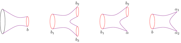
Figure 1: Elementary building blocks to construct any hyperbolic Riemann surfaces with conical singularities. When the corresponding surface has no AdS boundary, it can be constructed by three-holed spheres (with or without conical singularities) and the trumpet is needed to have asymptotic AdS boundary. The red circles represent the geodesic boundaries while the black one is asymptotic AdS boundary. The geodesic boundaries’ lengths and deficit angles are denoted by $b_{i}$ and $\alpha_{i}$, respectively.

Following the earlier work of Mirzakhani[19], the Weil-Petersson volumes we are interested in were studied in [20]. Indeed, the Weil-Petersson volumes of the moduli space of hyperbolic Riemann surfaces of genus $g$ with $m$ geodesic boundaries of lengths $(b_{1},\dots,b_{m})$ and $n$ conical singularities with deficit angles $(\alpha_{1},\dots,\alpha_{n})$ are given by [20]

$$V_{g,m,n}(b_{1},\dots,b_{m};\alpha_{1},\dots,\alpha_{n})=V_{g,m+n}(b_{1},\dots,b_{m},i(2\pi-\alpha_{1}),\dots,i(2\pi-\alpha_{n}))\,.$$ (2.4)

Here

$$V_{g,q}(b_{1},\dots,b_{q})=\sum_{|d|+\ell=3g+q-3}\frac{(2\pi^{2})^{\ell}}{2^{|d|}\ell!\,d_{1}!\dotsm d_{q}!}b_{1}^{2d_{1}}\dotsm b_{q}^{2d_{q}}\int_{\overline{{\cal M}}_{g,q}}\kappa^{\ell}\psi_{1}^{d_{1}}\dotsm\psi_{q}^{d_{q}},$$ (2.5)

is the Weil-Petersson volume of the moduli space of hyperbolic Riemann surfaces of genus $g$ with $q$ geodesic boundaries of lengths $(b_{1},\dots,b_{q})$[21]. In this expression $\Psi_{i}$ is the first Chern classes associated to the holes and $|d|=\sum_{i}d_{i}$. $\overline{{\cal M}}_{g,q}$ is the Deligne-Mumford compactification of ${\cal M}_{g,q}$ and $\kappa$ is the first Mumford-Morita-Miller class on the $\overline{{\cal M}}_{g,q}$ (see [16] for a quick review). It is then clear that the volume $V_{g,q}(b_{1},\dots,b_{q})$ is a polynomial in $b_{i}^{2}$ of degree $(3g-3+q)$.

Now, we have all the ingredients to compute the gravitational path integral over surfaces with $m$ boundaries. As we already mentioned, to evaluated the corresponding integrals one needs to consider two contributions. The first one comes from the Schwarzian modes associated to the asymptotic AdS boundary and the second part comes from the Weil-Petersson volumes. In the present case, and with the deformation (2.3), the contribution of the Schwarzian modes are given by [16]

$$Z_{\text{Disk}}(\beta)=\frac{e^{\frac{\pi^{2}}{\beta}}}{4\sqrt{\pi}\beta^{3/2}},\hskip 28.45274ptZ_{D(\alpha)}(\beta)=\frac{e^{\frac{(2\pi-\alpha)^{2}}{4\beta}}}{2\sqrt{\pi\beta}},\hskip 28.45274ptZ_{\text{trumpet}}(b,\beta)=\frac{e^{-\frac{b^{2}}{4\beta}}}{2\sqrt{\pi\beta}}\,.$$ (2.6)

Here we have assumed that the asymptotic boundary is a deformed circle with a renormalized length $\beta$. With this notation, one may compute the gravitational path integral for a connected geometry with $m$ boundaries which, in turns, corresponds to evaluating the connected part of the $m$-correlator

$$\langle Z(\beta)^{m}\rangle_{\rm conn}=\sum_{g=0}^{\infty}e^{-S_{0}\left(2g+m-2\right)}\hskip 2.84544ptZ_{g,m}(\beta),$$ (2.7)

where $S_{0}$ is the (renormalized) ground state entropy and (see also [16])

$$Z_{0,1}(\beta)\! \!\!=\!\! \!Z_{\text{Disk}}(\beta)$$ (2.10)

$$\!\!+\sum_{i=1}^{r}\varepsilon_{i}Z_{D(\alpha_{i})}(\beta)+\sum_{n=1}^{\infty}\sum_{i_{1},\dots,i_{n}=1}^{r}\frac{1}{n!}\hskip 2.84544pt\varepsilon_{i_{1}}\dotsm\varepsilon_{i_{n}}\int_{0}^{\infty}db\hskip 2.84544ptb\hskip 2.84544ptZ_{\text{trumpet}}(b,\beta)\hskip 2.84544ptV_{0,1;n}(b;\alpha_{i_{1}},\dots,\alpha_{i_{n}}),$$

$$Z_{0,2}(\beta)\! \!=\! \!\int_{0}^{\infty}db\hskip 2.84544ptb\hskip 2.84544ptZ^{2}_{\text{trumpet}}(b,\beta)$$ (2.14)

$$\!\!+\sum_{n=1}^{\infty}\sum_{i_{1},\dots,i_{n}=1}^{r}\frac{1}{n!}\hskip 2.84544pt\varepsilon_{i_{1}}\dotsm\varepsilon_{i_{n}}\int_{0}^{\infty}\bigg{(}\prod_{j=1}^{2}db_{j}\hskip 2.84544ptb_{j}\hskip 2.84544ptZ_{\text{trumpet}}(b_{j},\beta)\bigg{)}\hskip 2.84544ptV_{0,2;n}(b_{1},b_{2};\alpha_{i_{1}},\dots,\alpha_{i_{n}}),$$

$$Z_{g,m}(\beta)\! \!=\! \!\int_{0}^{\infty}\bigg{(}\prod_{j=1}^{m}db_{j}\hskip 2.84544ptb_{j}Z_{\text{trumpet}}(b_{j},\beta)\bigg{)}\hskip 2.84544ptV_{g,m}(b_{1},\dots,b_{m})$$

$$\!\!+\sum_{n=1}^{\infty}\sum_{i_{1},\dots,i_{n}=1}^{r}\frac{1}{n!}\varepsilon_{i_{1}}\dotsm\varepsilon_{i_{n}}\int_{0}^{\infty}\bigg{(}\prod_{j=1}^{m}db_{j}b_{j}\hskip 2.84544ptZ_{\text{trumpet}}(b_{j},\beta)\bigg{)}V_{g,m;n}(b_{1},\dots,b_{m};\alpha_{i_{1}},\dots,\alpha_{i_{n}}).$$

Here the first line of each expression represents the contribution of JT gravity whereas the second line is the contribution of the deformation of JT gravity. See the figure 2 for visual inspiration of how to write these expressions.

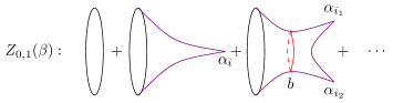
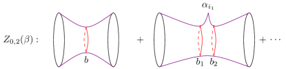
Figure 2: A visual representation of how to compute, for example, $Z_{0,1}(\beta)$ and $Z_{0,2}(\beta)$. The red circles represent the “suitable” geodesics.

Note that the factor of $\frac{1}{n!}$ comes from the fact that the location of conical singularities are indistinguishable [16]. Since the Weil-Petersson volumes are polynomials in $b_{i}$, one can perform the integration over $b$ in the expressions of $Z_{g,m}$ to find $Z_{g,m}$ as a function of $\beta$.

2.1 Gravity correlation functions

In this subsection we would like to compute the gravitational path integral using the above procedure. To proceed we shall first compute the disc partition function from which one may read the density of eigenvalues of the dual double-scaled random matrix model (assuming there is such a dual matrix model).

The first few geometries contributing to the disc partition function are depicted in figure 2. The corresponding partition function is[16]

$$\langle Z(\beta)\rangle_{g=0}=e^{S_{0}}Z_{0,1}(\beta)=\frac{e^{S_{0}}}{4\sqrt{\pi}\beta^{\frac{3}{2}}}\bigg{(}e^{\frac{\pi^{2}}{\beta}}+2\beta\sum_{i=1}^{r}\varepsilon_{i}e^{\frac{(2\pi-\alpha_{i})^{2}}{4\beta}}+2{(\sum_{i}^{r}\varepsilon_{i})^{2}\beta^{2}}+\frac{4}{3}(\sum_{i}^{r}\varepsilon_{i})^{3}\beta^{3}$$ (2.17)

(2.18)

$$\hskip 133.72795pt+\frac{4}{3}\bigg{(}4\pi^{2}\sum_{i}^{r}\varepsilon_{i}-3\sum_{i}^{r}\varepsilon_{i}(2\pi-\alpha_{i})^{2}\bigg{)}(\sum_{i}^{r}\varepsilon_{i})^{2}\beta^{2}\bigg{)}+\cdots,$$ (2.19)

which at low temperatures (large $\beta$) and small perturbations can be written in the following suggestive form

$$\langle Z(\beta)\rangle_{g=0}=\frac{e^{S_{0}}}{4\sqrt{\pi}\beta^{\frac{3}{2}}}\left(1+\beta(2\sum_{i}^{r}\varepsilon_{i})+\frac{1}{2!}{(2\sum_{i=1}^{r}\varepsilon_{i})^{2}\beta^{2}}+\frac{1}{3!}(2\sum_{i}^{r}\varepsilon_{i})^{3}\beta^{3}+\cdots\right)$$ (2.20)

(2.21)

$$\hskip 59.75095pt\approx\frac{e^{S_{0}}}{4\sqrt{\pi}\beta^{\frac{3}{2}}}e^{U(0)\beta}+\cdots,$$ (2.22)

where $U(0)=2\sum_{i=1}^{r}\varepsilon_{i}$. Assuming that there is a dual double-scaled matrix model, its corresponding density of eigenvalues can be obtained by making use of an inverse Laplace transformation [16]

$$\rho(E)\approx e^{S_{0}}\frac{\sqrt{E+U(0)}}{2\pi},$$ (2.23)

which is consistent with the general near threshold behavior of a hermitian matrix model if one identifies the threshold energy by $E_{0}=-U(0)$. Taking other terms into account one gets the same expression, though with a threshold energy with higher order correction[16].

It is also found useful to compute the contributions of higher genus terms to the partition function. Of course, in general this would be a very hard task. Nonetheless, for small enough perturbations, one could still make a progress in evaluating the corresponding quantity. Indeed, in this case one needs to compute the partition function given by (see also [22] for JT gravity)

$$\langle Z(\beta)\rangle=e^{S_{0}}Z_{0,1}(\beta)+\sum_{g=1}^{\infty}e^{-S_{0}(2g-1)}Z_{g,1}(\beta),$$ (2.24)

where

$$Z_{g,1}(\beta)=\frac{1}{2\sqrt{\pi\beta}}\int_{0}^{\infty}db\hskip 2.84544ptb\;e^{-\frac{b^{2}}{4\beta}}\bigg{(}V_{g,1}(b)+\sum_{n=1}^{\infty}\sum_{i_{1},\dots,i_{n}=1}^{r}\frac{1}{n!}\varepsilon_{i_{1}}\dotsm\varepsilon_{i_{n}}V_{g,1;n}(b;\alpha_{i_{1}},\dots,\alpha_{i_{n}})\bigg{)}.$$ (2.25)

Here using the equations (2.4) and (2.5) one has

$$V_{g,1}(b)=\sum_{d+\ell=3g-2}\frac{(2\pi^{2})^{\ell}}{2^{d}d!\ell!}b^{2d}\int_{\overline{{\cal M}}_{g,1}}\kappa^{\ell}\psi_{1}^{d},$$ (2.26)

(2.27)

$$V_{g,1;n}(b,\alpha_{i_{1}}\cdots,\alpha_{i_{n}})=\sum_{q+d+\ell=3g+n-2}\frac{(-1)^{q}(2\pi^{2})^{\ell}}{2^{d+q}d!\ell!q_{1}{!}\cdots q_{n}!}b^{2d}\prod_{j=1}^{n}(2\pi-\alpha_{i_{j}})^{2q_{j}}\int_{\overline{{\cal M}}_{g,1+n}}\kappa^{\ell}\psi_{1}^{d}\psi_{2}^{q_{1}}\cdots\psi_{1+n}^{q_{n}}\,.$$

with $q=\sum_{i=1}^{n}q_{i}$. Although it might be difficult to compute these volumes exactly, it is a relatively easy task to compute the leading order term in the low temperature limit by choosing the maximum value for $d$ in the above expressions – i.e. $d=3g-2$ for the first volume and $d=3g+n-2$ for the second one. Doing so, one gets

$$\int_{0}^{\infty}db\hskip 2.84544ptb\;e^{-\frac{b^{2}}{4\beta}}V_{g,1}(b)=\frac{1}{2\beta}\;\frac{(\beta^{3}/3)^{g}}{g!}+\cdots,\;\;\;\;\;\;\;\;\int_{0}^{\infty}db\,b\;e^{-\frac{b^{2}}{4\beta}}V_{g,1,n}(b)=(2\beta)^{n-1}\;\frac{(\beta^{3}/3)^{g}}{g!}+\cdots\;.$$ (2.28)

It is now straightforward to perform summations over $n$ and genus $g$ appearing in the equations (2.24) and (2.25) to arrive at

$$\langle Z(\beta)\rangle\simeq\frac{e^{S_{0}}}{4\sqrt{\pi}\beta^{\frac{3}{2}}}e^{\frac{\beta^{3}}{3}e^{-2S_{0}}}e^{U(0)\beta}+\cdots\,,$$ (2.29)

that should be compared with (2.20). One observes that the summation over $n$ results in $e^{U(0)\beta}$ factor, while the contribution of summing over all genus yields to the factor of ${\rm Exp}[\frac{1}{3}\beta^{3}e^{-2S_{0}}]$. Since we are working in the large $\beta$ limit, summing over all genus may not be convergent. Note, however that since we are working in the semi-classical gravity limit, and in order to be able to trust the gravity description, one should work in the large $S_{0}$ limit too. Therefore, to have control over the model, we will be working in the double scaling limit; in which both $\beta$ and $e^{S_{0}}$ are large while keeping $\beta^{\frac{3}{2}}e^{-S_{0}}$ fixed.

It is also interesting to study the connected part of $m$-correlators, $\langle Z(\beta)\rangle_{\rm conn}$, using the equation (2.7). To do so, one needs to evaluate $Z_{g,m}(\beta)$ given in the equation (2.10) which in turn requires to evaluate the Weil-Petersson volumes for arbitrary $m$. Of course, since we are interested in the low temperature limit of the $m$-point function, in the expression of Weil-Petersson volumes given in the equation(2.5), one may set $\ell=0$

$$V_{g,m}(b_{1},\dots,b_{m})=\sum_{|d|=3g+m-3}\frac{1}{2^{|d|}\,d_{1}!\dotsm d_{m}!}b_{1}^{2d_{1}}\dotsm b_{m}^{2d_{m}}\int_{\overline{{\cal M}}_{g,m}}\psi_{1}^{d_{1}}\dotsm\psi_{m}^{d_{m}}.$$ (2.30)

Similarly, for the case of $n$ conical singularities, the powers of $(2\pi-\alpha_{i})$ factors should also be set to zero in addition to $\ell$. Therefore, in this case the corresponding volumes do not depend on $\alpha_{i}$’s. More explicitly, one has

$$V_{g,m,n}(b_{1},\dots,b_{m};\alpha_{1},\dots,\alpha_{n})=\sum_{|d|=3g+m+n-3}\frac{1}{2^{|d|}\,d_{1}!\cdots d_{m}!}b_{1}^{2d_{1}}\cdots b_{m}^{2d_{m}}\int_{\overline{{\cal M}}_{g,m+n}}\psi_{1}^{d_{1}}\cdots\psi_{m}^{d_{m}}.$$ (2.31)

Plugging the above expressions into the equation (2.10) and performing the integrals over $b_{I}$’s and, moreover, taking into account the following identity (see for example [24])

$$\int_{\overline{{\cal M}}_{g,m+1}}\psi_{1}^{d_{1}}\cdots\psi_{m}^{d_{m}}=\sum_{k=1}^{m}\;\;\;\int_{\overline{{\cal M}}_{g,m}}\psi_{1}^{d_{1}}\cdots\psi_{k}^{d_{k}-1}\cdots\psi_{m}^{d_{m}},$$ (2.32)

one gets

$$Z_{g,m}(\beta)\! \!=\! \!\left(\frac{\beta}{\pi}\right)^{\frac{m}{2}}\bigg{(}\sum_{|d|=3g+m-3}(2\beta)^{3g+m-3}\int_{\overline{{\cal M}}_{g,m}}\psi_{1}^{d_{1}}\cdots\psi_{m}^{d_{m}}$$

$$\hskip 56.9055pt+\sum_{i_{1},\cdots,i_{n}=1}^{r}\frac{2^{n}}{n!}\varepsilon_{i_{1}}\cdots\varepsilon_{i_{n}}\;m^{n}\;\beta^{n}\sum_{|d|=3g+m-3}(2\beta)^{3g+m-3}\int_{\overline{{\cal M}}_{g,m}}\psi_{1}^{d_{1}}\cdots\psi_{m}^{d_{m}}\bigg{)}.$$

Inserting this expression in the equation (2.7) one arrives at

$$\langle Z(\beta)^{m}\rangle_{\rm conn}=\left(\frac{\beta e^{-\frac{2S_{0}}{3}}}{\pi}\right)^{\frac{m}{2}}e^{mU(0)\beta}\sum_{g=0}^{\infty}\sum_{|d|=3g+m-3}\prod_{i=1}^{m}t_{i}^{d_{i}}\int_{\overline{{\cal M}}_{g,m}}\psi_{1}^{d_{1}}\cdots\psi_{m}^{d_{m}},$$ (2.34)

where $t_{i}=2\beta e^{-\frac{2S_{0}}{3}}$ for all $i$’s. Actually, the summations over all genus and all possible partitions of $d_{i}$ appearing in this expression have been evaluated in [27] that may be written as follows

$$\sum_{g=0}^{\infty}\sum_{|d|=3g+m-3}\prod_{i=1}^{m}t_{i}^{d_{i}}\int_{\overline{{\cal M}}_{g,m}}\psi_{1}^{d_{1}}\cdots\psi_{m}^{d_{m}}\!\! \!\!=\!\! \!\!\left(\frac{2\pi}{t_{i}}\right)^{\frac{m}{2}}\sum_{\rm all\;possible\;k-partitions\;of\;m}(-1)^{k-1}{\cal E}_{k}(m_{1},\cdots,m_{k})$$ (2.37)

$$=\left(\frac{2\pi}{t_{i}}\right)^{\frac{m}{2}}\bigg{(}{\cal E}_{1}(m)-m\;{\cal E}_{2}(m-1,1)+\cdots+(1)^{m-1}(m-1)!\;{\cal E}_{m}(1,\cdots,1)\bigg{)},$$

where ${\cal E}_{k}$ is

$${\cal E}_{k}(m_{1},\dots,m_{k})=\left(\frac{e^{S_{0}}}{\sqrt{\pi}}\right)^{k}\;\frac{e^{\frac{\sum_{i}m_{i}^{3}}{3}\beta^{3}e^{-2S_{0}}}}{\beta^{\frac{k}{2}}\prod_{i=1}^{k}m_{i}^{\frac{1}{2}}}\;\int_{-\infty}^{0}\prod_{j=1}^{k}dx_{j}\;e^{\sum_{i=1}^{k}(x_{i}+x_{i-1})m_{i}\beta}e^{-\sum_{i=1}^{k}\frac{(x_{i}-x_{i-1})^{2}}{4m_{i}\beta e^{-2S_{0}}}}.$$ (2.38)

Note that in the summation over all possible $k$-partitions of $m$, one should also take into account the symmetric factor for each term as indicated in the second line of (2.37). Plugging this expression into the equation (2.34) one finds

$$\langle Z(\beta)^{m}\rangle_{\rm conn}=\sum_{\rm all\;possible\;k-partitions\;of\;m}(-1)^{k-1}{\cal Z}(m_{1},\dots,m_{k}),$$ (2.39)

with

$${\cal Z}(m_{1},\dots,m_{k})=e^{mU(0)\beta}{\cal E}_{k}(m_{1},\dots,m_{k}).$$ (2.40)

Note that in this summation the proper symmetric factor for each term, as mentioned, should be also taken into account.

2.2 Matrix model description

In this section, assuming that the deformed JT gravity (2.1) is dual to a double-scaled random matrix model, we would like to study a possible dual matrix model that reproduces the desired results of the gravity computations.

It is worth mentioning that the main technical reason of having a duality between a double-scaled matrix model and JT gravity shown in [1] was that upon a Laplace transformation Mirzakhani’s recursion relation [28] maps to the recursion relation of a double-scaled matrix model[29]. The corresponding recursion relation could fix all correlators in all orders in genus expansion in terms of the inverse Laplace transformation of disc partition function (the leading order density of eigenvalues). So that, to all orders in $e^{-S_{0}}$ expansion the arbitrary correlation functions, $\langle Z(\beta_{1})\cdots Z(\beta_{n})\rangle$, of JT gravity coincides with that of a double-scaled random matrix ensemble. Since the model we have been considering in this paper is a deformation of JT gravity one would naturally expect that a similar procedure could also work for the deformed JT duality[17].

It was also argued that the double-scaled matrix model relevant for JT gravity has a certain similarity with minimal string theory [1]. The connection with minimal string theory and its possible relation with the old version of matrix model of 2-dimensional gravity has also been studied in [22] and [30, 31, 32]. An advantage of working with minimal string theories is that one may have a better control of non-perturbative effects of gravity in this context.

Following [30] in this subsection we shall explore the above procedure for deformed JT gravity. To proceed, we note that in this context the partition function of desired matrix integrals may be viewed as the partition function of a one dimensional quantum system with the following Hamiltonian [33, 34, 35]

$$H=-e^{-2S_{0}}\frac{\partial^{2}}{\partial x^{2}}+u(x),$$ (2.41)

where $u(x)$ is a potential to be determined for the model of interest. Indeed, the corresponding potential satisfies a non-linear ordinary differential equation known as string equation[36]

$$(u-E_{0})\mathcal{R}^{2}-\frac{e^{-2S_{0}}}{2}\mathcal{R}\mathcal{R}^{\prime\prime}+\frac{e^{-2S_{0}}}{4}(\mathcal{R}^{\prime})^{2}=0,$$ (2.42)

where

$$\mathcal{R}\equiv\sum_{k=0}^{\infty}t_{k}R_{k}[u]+x.$$ (2.43)

Here ${R}_{k}[u]$ is a $k$-th polynomial of $u(x)$ and its derivatives with respect to $x$ defined in [36]. In particular in our notation

$$R_{0}[u]=1,\;\;\;\;\;\;\;R_{1}[u]=u(x),\;\;\;\;\;\;\;\;{R}_{2}[u]=u(x)^{2}-\frac{1}{3}e^{-2S_{0}}u^{\prime\prime}(x).$$ (2.44)

To find the coefficients $t_{k}$’s for the deformed JT gravity one may use that the fact that for $x=0$ setting $R_{k}=E_{0}^{k}$ then ${\cal R}=0$ reduces to an algebraic equation from which one could find the exact threshold energy $E_{0}$.

To find the corresponding algebraic equation we note that at low temperatures the leading order density of eigenvalues is given by $\rho_{0}(E)\sim\sqrt{E-E_{0}}$, which in turns, fixes the general form of the disc partition function for large $\beta$ as follows [16]

$$\langle Z(\beta)\rangle_{g=0}=\frac{e^{S_{0}}e^{-\beta E_{0}}}{4\sqrt{\pi}\beta^{\frac{3}{2}}}\bigg{\{}e^{\beta E_{0}}\bigg{(}e^{\frac{\pi^{2}}{\beta}}+2\beta\sum_{i=1}^{r}\varepsilon_{i}e^{\frac{(2\pi-\alpha_{i})^{2}}{4\beta}}+2{(\sum_{i}^{r}\varepsilon_{i})^{2}\beta^{2}}+\frac{4}{3}(\sum_{i}^{r}\varepsilon_{i})^{3}\beta^{3}$$ (2.45)

(2.46)

$$\hskip 119.50157pt+\frac{4}{3}\bigg{(}4\pi^{2}\sum_{i}^{r}\varepsilon_{i}-3\sum_{i}^{r}\varepsilon_{i}(2\pi-\alpha_{i})^{2}\bigg{)}(\sum_{i}^{r}\varepsilon_{i})^{2}\beta^{2}\bigg{)}+\cdots\bigg{\}},$$ (2.47)

with a constraint that coefficients of the positive powers of $\beta$ in the brackets should vanish. In particular from vanishing of the coefficient of $\beta$ one gets [16, 17]

$$\frac{\sqrt{E_{0}}}{2\pi}I_{1}(2\pi\sqrt{E_{0}})+\sum_{i=1}^{r}\varepsilon_{i}I_{0}((2\pi-\alpha_{i})\sqrt{E_{0}})=0,$$ (2.48)

where $I_{0}$ and $I_{1}$ are modified Bessel functions. Using the series expansion of the modified Bessel functions, one can read the coefficients $t_{k}$’s as follows

$$t_{k}=\frac{1}{2}\frac{\pi^{2k-2}}{k!(k-1)!}+\sum_{i=1}^{r}\varepsilon_{i}\frac{(2\pi-\alpha_{i})^{2k}}{2^{2k}(k!)^{2}},\;\;\;\;\;\;\;\;t_{0}=\sum_{i=1}^{r}\varepsilon_{i}$$ (2.49)

In general, using the string equation, one could find the potential associated to the Hamiltonian of the quantum system (2.41). Then, one could in principle find the spectrum of the Hamiltonian from which one may evaluate the spectral density non-perturbatively.

Of course, in general it is a very hard task. We note, however, that at low temperatures one could find the potential perturbatively. Indeed, this is exactly the Airy limit in which the corresponding matrix model is controlled by the universal behavior of the edge of the classical density of eigenvalues[37].

The potential we are interested in can be obtained by the solution of $\mathcal{R}=0$ which at leading order results in $u(x)=-2Cx+E_{0}$, with

$$C=1-\pi U^{\prime}(0)-\frac{1}{4}U^{\prime\prime}(0),\;\;\;\;\;\;\;\;E_{0}=-U(0)+\frac{1}{2}\pi^{2}U^{2}(0)+\pi U(0)U^{\prime}(0)+\frac{1}{4}U(0)U^{\prime\prime}(0)\,,$$ (2.50)

where

$$U^{\prime}(0)=-2\sum_{i=1}^{r}\varepsilon_{i}\alpha_{i},\;\;\;\;\;\;\;\;\;\;\;U^{\prime\prime}(0)=2\sum_{i=1}^{r}\varepsilon_{i}\alpha_{i}^{2}.$$ (2.51)

It is then clear that the Hamiltonian gets a shift with $E_{0}$. Therefore one arrives at the following equation for the wave function

$$\left[-\frac{e^{-2S_{0}}}{2C}\frac{\partial^{2}}{\partial x^{2}}-x\right]\psi(E,x)=\frac{E-E_{0}}{2C}\,\psi(E,x)\,,$$ (2.52)

which could be solved to find

$$\psi(E,x)=e^{\frac{2S_{0}}{3}}(2C)^{\frac{1}{3}}\operatorname{Ai}(\xi),\;\;\;\;\;\;{\rm with}\;\;\xi=-e^{\frac{2S_{0}}{3}}(2C)^{\frac{1}{3}}\left(x+\frac{E-E_{0}}{2C}\right).$$ (2.53)

Using this wave function, the corresponding density of eigenvalues,

$$\rho_{\rm Airy}(E)=e^{\frac{4S_{0}}{3}}(2C)^{\frac{2}{3}}\int_{-\infty}^{0}dx\;{\rm Ai}^{2}\left[-e^{\frac{2S_{0}}{3}}(2C)^{\frac{1}{3}}\left(x+\frac{E-E_{0}}{2C}\right)\right],$$ (2.54)

reads

$$\rho_{\text{Airy}}(E)=e^{\frac{2S_{0}}{3}}(2C)^{\frac{1}{3}}\left(\text{Ai}^{\prime 2}(\eta)-\eta\text{Ai}^{2}(\eta)\right),\;\;\;\;\;{\rm with}\;\;\;\eta=-e^{\frac{2S_{0}}{3}}(2C)^{\frac{1}{3}}\;\frac{E-E_{0}}{2C}.$$ (2.55)

In particular, at leading order in $e^{-S_{0}}$ it is

$$\rho_{\text{Airy}}(E)\approx\frac{e^{S_{0}}}{\pi}\;\sqrt{E-E_{0}},\;\;\;\;\;\;\;\;\;\;\;\;\;{\rm for}\;\;E\geq E_{0},$$ (2.56)

reproducing (2.23). It is worth noting that although the above leading order expression for energy density is valid for $E\geq E_{0}$, the full expression (2.55) has a non-zero support on the entire real axis. In fact, in what follows, in order to compare the results with those obtained from the geometrical computations we will take all integral over the entire real axis, though in general one should be careful about the spectrum below the threshold energy [30, 32]. We will come back to this point in the next section where we shall compute the free energy.

Plugging the energy density (2.55) into the equation (2.2) one gets (see below for more details)

$$\langle Z(\beta)\rangle=\frac{e^{S_{0}}}{2\sqrt{\pi}\beta^{\frac{3}{2}}}e^{\frac{1}{3}\beta^{3}e^{-2S_{0}}}e^{-\beta E_{0}},$$ (2.57)

which is the same as that obtained from gravity computations (2.29).

In what follows we will compute $\langle Z(\beta)^{m}\rangle_{\rm conn}$ to all orders in genus expansion for arbitrary $m$ in the low temperature limit using the Airy wave function of the dual matrix model considered above. To proceed, we note that the connected $m$ point function consists of several terms given by [38](see also[39, 40])

$$\langle Z(\beta)^{m}\rangle_{\rm conn} = {\rm Tr}\left(e^{-m\beta H}P\right)-m{\rm Tr}\left(e^{-(m-1)\beta H}Pe^{-\beta H}P\right)+\cdots$$ (2.59)

$$+(-1)^{m-1}(m-1)!\;{\rm Tr}\left(e^{-\beta H}Pe^{-\beta H}P\cdots Pe^{-\beta H}P\right)$$

where $P$ is the projection operator

$$P=\int_{-\infty}^{0}dx\;|x\rangle\langle x|.$$ (2.60)

To evaluate this connected $m$ point function, one generally needs to compute the following quantity

$${\cal Z}(m_{1},\dots,m_{k})={\rm Tr}\left(e^{-m_{1}\beta H}Pe^{-m_{2}\beta H}P\cdots Pe^{-m_{k}\beta H}P\right)$$ (2.61)

with the condition $\sum\limits_{i=1}^{k}m_{i}=m$. By making use of the wave function $H|\psi\rangle=E|\psi\rangle$ and the fact that $\int dE|\psi\rangle\langle\psi|=1$, one could rewrite the traces in terms of integrals in order to arrive at

$${\cal Z}(m_{1},\dots,m_{k})=\int_{-\infty}^{0}\prod_{j=1}^{k}dx_{j}\prod_{i=1}^{k}\int_{-\infty}^{\infty}dE_{i}\;\;e^{-m_{i}\beta E_{i}}\;\psi(E_{i},x_{i-1})\psi^{*}(E_{i},x_{i})\,,$$ (2.62)

where

$$\psi(E_{i},x_{j})=e^{\frac{2S_{0}}{3}}2^{\frac{1}{3}}\operatorname{Ai}\left[-e^{\frac{2S_{0}}{3}}2^{\frac{1}{3}}\left(x_{j}+\frac{E_{i}-E_{0}}{2}\right)\right].$$ (2.63)

Here we have used a notation in which $x_{0}=x_{k}$. Plugging this wave function into the above equation and using a proper change of the coordinates, one gets

$${\cal Z}(m_{1},\dots,m_{k})=\left(e^{\frac{2S_{0}}{3}}2^{\frac{4}{3}}\right)^{k}\;e^{-m\beta E_{0}}\int_{-\infty}^{0}\prod_{j=1}^{k}dx_{j}$$ (2.64)

$$\hskip 28.45274pt\times\prod_{i=1}^{k}\int_{-\infty}^{\infty}dE_{i}\;\;e^{e^{\frac{-2S_{0}}{3}}2^{\frac{2}{3}}m_{i}\beta E_{i}}{\rm Ai}\left(E_{i}-e^{\frac{2S_{0}}{3}}2^{\frac{1}{3}}x_{i-1}\right){\rm Ai}\left(E_{i}-e^{\frac{2S_{0}}{3}}2^{\frac{1}{3}}x_{i}\right).$$

By making use of the following identity

$$\int_{-\infty}^{\infty}e^{xy}\text{Ai}(x+a)\text{Ai}(x+b)\,dx=\frac{1}{2\sqrt{\pi y}}\exp\left(\frac{y^{3}}{12}-\frac{a+b}{2}y-\frac{(a-b)^{2}}{4y}\right)\,,$$ (2.65)

one may perform the integration over $E_{i}$’s to get

$${\cal Z}(m_{1},\dots,m_{k})=e^{-m\beta E_{0}}\;{\cal E}_{k}(m_{1},\dots,m_{k}),$$ (2.66)

where ${\cal E}_{k}(m_{1},\dots,m_{k})$ is given by (2.38). Therefore, one gets the same expression for connected $m$ corrlators as given in the equation (3.19). Clearly, for $k=1$ this reduces to that of (2.57).

It is worth noting that the connected $m$ point function at low temperatures decays as $\beta^{-3/2}$ while the partition function of fully disconnected topologies with $m$ boundaries goes as $\beta^{-3m/2}$. It indicates that at low temperatures the physics is dominated by the connected topologies.

3 Free energy for Deformed JT gravity

In the previous section, we have considered a particular deformation of JT gravity whose dual theory is shown to be a Hermitian random matrix model [16, 17]. We have also computed the partition function of this model at low temperatures to all orders in genus expansion for small perturbations. We have observed that the resultant partition function (in the low temperature limit) is in agreement with that obtained from the Airy limit of a Hermitian matrix model.

Having found the partition function, it is then natural to proceed to study other relevant quantities. One of the most fundamental quantities one may study is the free energy. Thus, in what follows, we will study free energy following the procedure considered in [6]. Of course, since the computations are very similar to that of the mentioned paper in the first part of this section, we will be very brief and the reader is referred to the paper for more details.

An immediate way to compute the free energy is to consider the logarithm of connected partition function that computes the annealed free energy

$$F_{\text{ann}}=-T\log\langle Z(\beta)\rangle=-T\log\langle Z(\beta)\rangle\,,$$ (3.1)

which, using equation (2.29), is given by

$$F_{\text{ann}}=-T{S_{0}}-T\log\frac{T^{\frac{3}{2}}}{4\sqrt{\pi}}-\frac{1}{3T^{2}}e^{-2S_{0}}-{U(0)}\,.$$ (3.2)

Using the full expression for the partition function, given in equation (2.7), one can numerically evaluate the annealed free energy and the result of this computation is depicted in figure 3. To compare this result with that of JT gravity, we have also plotted the corresponding free energy for this model.

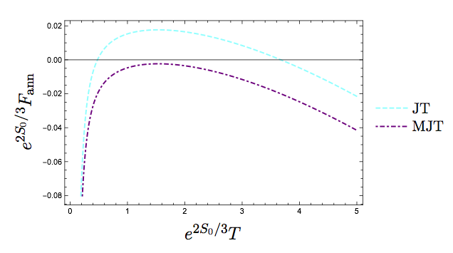
Figure 3: The annealed free energy for $S_{0}=7$ and $U(0)=1/50$. Apart from the divergence for $\beta\gg 1$, the local maximum is still present even by the inclusion of higher genus corrections (doubly non-perturbative effects).

It is worth mentioning that this figure cannot be trusted for high temperatures. Indeed, we should emphasize that the main lesson one can learn from this figure is that the annealed free energy diverges and also exhibits a maximum at low temperatures. Therefore, the annealed free energy is not a useful quantity to be considered for the system since it is both non-monotonic and divergent. Indeed, as it is well-known in condensed matter physics literature, a better quantity one may define is the quenched free energy which we shall study it in what follows.

To compute the quenched free energy for JT gravity, the authors of [6] have used a certain replica trick. In the present case, we will consider the same method to compute the quench free energy. To proceed, one should consider the gravitational path integral on $m$ copies of the boundary $B$ and then the analytical continuation to $m=0$ should be performed

$$F_{\rm que}=-T\langle\log Z(\beta)\rangle=-T\lim_{m\rightarrow 0}\frac{1}{m}\left(\langle Z(\beta)^{m}\rangle-1\right)\,.$$ (3.3)

Although the above expression is a concrete statement, in practice it is very hard to implement. The main point in this calculation is that since the Weil-Peterson volumes are only well-defined for integer $m$, it is not clear how to extend their definition to the case of non-integer $m$. Therefore, the analytical continuation for general $m$, and in particular the limit $m\rightarrow 0$, might not be well-imposed.

The way the authors of [6] proposed to circumvent this difficulty was to define a “truncated free energy” by evaluating the gravitational path integral over geometries which include only topologies that connect up to M boundaries. More precisely, one may define $\langle Z(\beta)^{m}\rangle_{M}$ as follows

$$\sum_{m=0}^{\infty}\frac{t^{m}}{m!}\langle Z(\beta)^{m}\rangle_{M}={\rm exp}\left(\sum_{m=1}^{M}\frac{t^{m}}{m!}\langle Z(\beta)^{m}\rangle_{\rm conn}\right),$$ (3.4)

and then the truncated free energy is defined by

$$\bar{F}_{M}=-T\lim_{m\rightarrow 0}\frac{1}{m}\left(\langle Z(\beta)^{m}\rangle_{M}-1\right)\,.$$ (3.5)

For more detail the reader is refereed to [6]. Following this paper, let us considered the following analytic continuation of $m$ factorial

$$m!=\int_{0}^{\infty}dt\hskip 2.84544pte^{-t}\hskip 2.84544ptt^{m},\;\;\;\;\;\;\;\;\;\;\frac{1}{m!}=\frac{1}{2\pi i}\oint_{C\equiv\text{Hankel countour}}dz\hskip 2.84544pte^{z}z^{-(m+1)}.$$ (3.6)

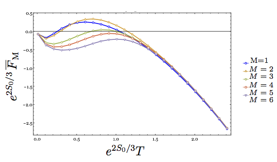
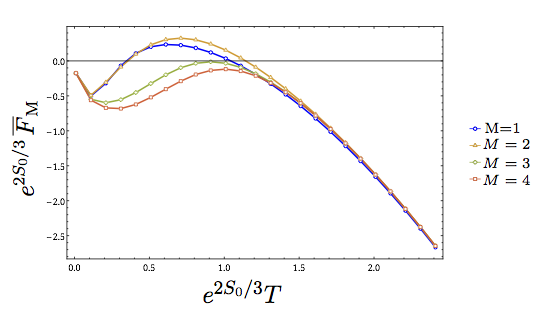
Figure 4: Left: The (first order perturbation) quenched free energy $\overline{F}_{M}$ for $S_{0}=7$, $\epsilon=1/100$ and $\alpha=3\pi/2$ using topologies with genus up to one and various $M=1,2,3,4,5,6$. right: The (first order perturbation) quenched free energy $\overline{F}_{M}$ for $S_{0}=7$, $\epsilon=1/100$ and $\alpha=3\pi/2$ using topologies with genus up to two and various $M=1,2,3,4$.

Then, the truncated free energy is found to be [6]

$$\overline{F}_{M}=-\text{T}\hskip 2.84544pt\text{Re}\int\bigg{(}\prod_{k=1}^{M-1}d\mu(t_{k},z_{k})\bigg{)}\frac{1}{M!}\sum_{j_{1}=0}^{1}...\sum_{j_{M-1}=0}^{M-1}\log\mathcal{A}_{j_{1}...j_{M-1}}^{(M)}(\{t_{k},z_{k}\})$$ (3.7)

where

$$d\mu(t_{k},z_{k})=\int_{0}^{\infty}dt_{k}\oint dz_{k}\hskip 1.42262pt\frac{e^{z-t}}{2\pi iz},$$ (3.8)

$$\mathcal{A}_{j_{1}...j_{M-1}}^{(M)}(\{t_{k},z_{k}\})=\mathcal{P}_{\text{conn},1}(\beta)+\sum_{k=2}^{M}e^{\frac{2\pi i}{k}j_{k-1}}\bigg{(}\frac{\langle Z(\beta)^{k}\rangle_{\rm conn}}{k!\hskip 2.84544ptz_{k-1}}\bigg{)}^{\frac{1}{k}}t_{k-1}.$$ (3.9)

Therefore, the quenched free energy is defined as

$$F_{\rm que}=\lim_{M\rightarrow\infty}\overline{F}_{M}.$$ (3.10)

It is worth mentioning that the resultant free energy depends on the choice of contours, $C_{k}$, of which the integration over $z_{k}$’s is performed (needed for the analytic continuation of the $\Gamma(m+1)\equiv m!$). Although, using this definition of analytic continuation makes it possible to compute the quenched free energy numerically, in practice it is very time consuming (if not impossible) to evaluate large $M$ limit of the truncated free energy. The numerical results for few $M$’s are depicted in the figure 4.

As it is clear from figure 4, the replica wormholes have significantly changed the low temperature behavior of the free energy, although it still has its undesirable feature of being non-monotonic! One reason for this odd behavior could be that the quenched free energy, by definition, is supposed to be computed in the large $M$ limit. Therefore, even though the plots get smoothed already in small $M$’s, we should not expect to have the correct behavior for small $M$’s.

Of course, one could still doubt about the analytic continuation of $m$ and the way the replica trick is used in the case. This issue has been extensively explored in [6] where the results were interpreted as an evidence for the necessity of replica symmetry breaking. We note, however, that since the observation is based on the numerical computations, the results may not be conclusive enough. It would be interesting if one could have a better understanding of low temperature behavior of the free energy and in particular if one could do some analytic computations. This is, indeed, the subject of the next subsection.

3.1 Free energy at low temperatures

As we have seen in the previous section, the deformed JT gravity at low temperatures could be described by a matrix model in the Airy limit, in which the corresponding matrix model is controlled by the universal behavior of the edge of the classical density of eigenvalues. Using this observation, in what follows we would like to compute the quenched free energy of this model at low temperatures by making use of the Airy wave function.

To proceed, one needs to compute the gravitational path integral on geometries with $m$ boundaries, $\langle Z(\beta)^{m}\rangle$. In general, the gravitational path integral involves a sum over all topologies connecting $m$ boundaries and the resultant quantity should be interpreted as being dual to an ensemble average (at least in two dimensions). In particular, for $m=1$, this is actually ensemble average of partition function studied in the previous section.

The obtained partition function may be used to compute the annealed free energy that is essentially the same as that in (3.1), showing pathological properties for free energy at the low temperatures. This, in turn, would indicate the necessity of using replica trick to include the connected topologies.

For $m$ disconnected boundaries , there are different topologies contributing to gravitational path integral. If the gravitational path integral was computed for the fully disconnected topology, one had $\langle Z(\beta)^{m}\rangle=\langle Z(\beta)\rangle^{m}$. We note, however, that in the gravitational theory we are considering, this is not the case. Therefore, we will have to sum over all topologies. The sum starts from the fully disconnected geometry and will end up with the fully connected one. Schematically, one may write

$$\langle Z(\beta)^{m}\rangle=\langle Z(\beta)\rangle^{m}+\langle Z(\beta)\rangle^{m-2}\langle Z(\beta)^{2}\rangle_{\rm conn}+\cdots+\langle Z(\beta)^{m}\rangle_{\rm conn}\,.$$ (3.11)

The first term is just the $m$-th power of the partition function we have computed in the previous section that decays as $\beta^{-3m/2}$ for large $\beta$. The fully connected term is also computed in the previous section where one observed that at leading order it decays as $\beta^{-3/2}$ at low temperatures.

For fixed $m\geq 1$ the connected topologies dominate at low temperatures while at high temperatures, the fully disconnected one plays an important role. The temperature in which the role of connected and disconnected topologies gets exchanged is given in terms of the extremal entropy $e^{S_{0}}$. In fact, the situation is very similar to that of the island formula for fine grained entropy of evaporating black holes [4, 5]. Indeed, in our study, $\beta^{-1}$ plays the role of the matter degrees of freedom in that context.

We note, however, that since we are interested in using replica trick to evaluate free energy in which one needs to analytically continue $m$ for non-integer numbers and in particular taking $m\ll 1$ limit, the situation might be more involved. At this point, all we would like to emphasize is that taking the $m\rightarrow 0$ is tricky and one should keep track of how to implement this limit.

In the previous section, we have computed the connected part of the gravitational path integral with $m$ boundaries at low temperatures. In principle, one could plug the result into the equation (3.3) to find the quenched free energy. Doing so, one gets

$$F_{que}\approx-T\lim_{m\rightarrow 0}\frac{1}{m}\left(Z(\beta^{m})_{\rm conn}-1\right)\sim\lim_{m\rightarrow 0}\left(-\frac{T^{\frac{5}{2}}e^{S_{0}}}{\sqrt{\pi}m^{\frac{5}{2}}}e^{\frac{m}{3}\beta^{3}e^{-2S_{0}}}e^{-m\beta E_{0}}+\frac{T}{m}\right){.}$$ (3.12)

The above expression seems divergent and leads to an ill-defined quantity. Keeping in mind the above discussions on analytic continuation, our understanding of this undesired result is that the naive replica trick and $m\rightarrow 0$ limit we have used are not precise enough.

To further explore this point, we will follow the procedure which has been recently considered by [39] in the remainder of this section. To begin, let us note that the spectral density in the Airy limit, (2.55), is non-zero at the threshold energy:

$$\rho_{\rm Airy}(E_{0})=\frac{e^{\frac{2S_{0}}{3}}2^{\frac{1}{3}}}{3^{\frac{2}{3}}\Gamma\left(\frac{1}{3}\right)^{2}}\,.$$ (3.13)

Note that non-zero energy density at threshold energy should be generated by non-perturbative quantum effects. In particular, looking at the leading order (g=0) expression for the spectral density, (2.56), one observes that it vanishes at the threshold energy.

Having a finite and non-zero density, it is natural to study the thermal properties of this model around the threshold energy (specially if one wants to work in the low temperature approximation). Being at a thermal state, an appropriate way to identify the state is to give its spectral density which is defined in (2.54). This expression can be written in the following form

$$\rho_{\rm Airy}(\mu,E)=e^{\frac{2S_{0}}{3}}2^{\frac{1}{3}}\int^{2^{\frac{1}{3}}e^{\frac{2{S_{0}}}{3}}\mu}_{0}dx\;{\rm Ai}^{2}\left[x-e^{\frac{2S_{0}}{3}}2^{-\frac{2}{3}}\left({E-E_{0}}\right)\right],$$ (3.14)

where $\mu>0$ is a cutoff whose significance will be become clear latter. It is worth mentioning that $\rho_{\rm Airy}(E_{0})=\lim_{\mu\rightarrow\infty}\rho_{\rm Airy}(\mu,E_{0})$. Of course, in what follows we shall consider the opposite limit, $\mu\rightarrow 0$, in which one has $\rho_{\rm Airy}(\mu,E)\sim\mu$. The reason for taking small $\mu$ limit is that in order to maintain the validity of our approximation for expression of the wave function around the threshold energy the range of $x$ should be small.

As we have already mentioned in the previous section, although the energy density defined in the Airy limit (given in terms of the Airy function) may be defined along all real axis, in order to compute the partition function one needs to truncate the energy for $E\geq E_{0}$. In fact, motivated by that of the JT gravity [1] one would expect that there are non-perturbative instabilities which could be connected to the fact that there are non-perturbative contributions to the spectral density for $E<E_{0}$. In the context of JT gravity, a remedy to avoid the instability was proposed in [30, 32] that essentially enforces us to work with the Airy function with the spectrum truncated at $E=0$. Following this observation in what follows we will consider the case where the spectrum is truncated for $E\geq E_{0}$.

It is important to mention that restraining ourselves to $E\geq E_{0}$ limit, the truncated spectrum would change the leading order behavior of the partition function significantly. To see this, let us compute the partition function around the threshold energy as follows

$$\langle Z(\beta)\rangle=\int_{E_{0}}^{\infty}dE\;e^{-\beta E}\rho_{\rm Airy}(\mu,E_{0})=\frac{\rho_{\rm Airy}(\mu,E_{0})}{\beta}e^{-\beta E_{0}}.$$ (3.15)

On the other hand, since we are at low energies, one should also take $\mu\rightarrow 0$ limit

$$\rho_{\rm Airy}(\mu,E_{0})\approx\frac{2^{\frac{2}{3}}e^{\frac{4{S_{0}}}{3}}}{3^{\frac{4}{3}}\Gamma\left(\frac{2}{3}\right)^{2}}\;\mu,\;\;\;\;\;\;\;\;{\rm for}\;\;\mu\approx 0\,.$$ (3.16)

so that

$$\langle Z(\beta)\rangle\approx\frac{2^{\frac{2}{3}}}{3^{\frac{4}{3}}\Gamma\left(\frac{2}{3}\right)^{2}}\frac{e^{\frac{4{S_{0}}}{3}}\mu}{\beta}e^{-\beta E_{0}}.$$ (3.17)

Note that, unlike the equation (2.20), the leading order of the above partition function decays as $\beta^{-1}$ at low temperatures. It is also useful to evaluate ${\cal Z}(m_{1},\dots,m_{k})$ in this limit:

$${\cal Z}(m_{1},\dots,m_{k})=\frac{\rho^{k}_{\rm Airy}(\mu,E_{0})}{\beta^{k}\prod_{i=1}^{k}m_{i}}\;e^{-m\beta E_{0}}.$$ (3.18)

Then, it is straightforward to compute the gravitational path integral over geometries with $m$ boundaries (3.11)

$$\langle Z(\beta)^{m}\rangle=\bigg{\{}\bigg{(}\frac{\rho^{m}_{\rm Airy}(\mu,E_{0})}{\beta^{m}}\bigg{)}+\frac{m(m-1)}{2}\bigg{(}\frac{\rho^{m-1}_{\rm Airy}(\mu,E_{0})}{2\beta^{m-1}}-\frac{\rho^{m}_{\rm Airy}(\mu,E_{0})}{\beta^{m}}\bigg{)}+\cdots$$ (3.19)

(3.20)

$$\hskip 28.45274pt+m\bigg{(}\frac{\rho^{2}_{\rm Airy}(\mu,E_{0})}{(m-1)\beta^{2}}-(m-1)\frac{\rho^{3}_{\rm Airy}(\mu,E_{0})}{\beta^{3}(m-2)}\;+\cdots+(-1)^{m-2}(m-2)!\frac{\rho^{m}_{\rm Airy}(\mu,E_{0})}{\beta^{m}}\bigg{)}$$ (3.21)

(3.22)

$$\hskip 28.45274pt+\bigg{(}\frac{\rho_{\rm Airy}(\mu,E_{0})}{m\beta}\;-m\frac{\rho^{2}_{\rm Airy}(\mu,E_{0})}{\beta^{2}(m-1)}\;+\cdots+(-1)^{m-1}(m-1)!\frac{\rho^{m}_{\rm Airy}(\mu,E_{0})}{\beta^{m}}\;\bigg{)}\bigg{\}}e^{-m\beta E_{0}}.$$

Here, the first term corresponds to the fully disconnected piece while the last one comes from the fully connected term. The other terms are a mixture of the connected and disconnected components. In particular, the two other terms that are explicitly written in the above equation, are associated with the following terms

$$\langle Z(\beta)\rangle^{m-2}\langle Z(\beta)^{2}\rangle_{\rm conn}\;,\;\;\;\;\;\;\;\;\;\;\;\;\langle Z(\beta)\rangle\langle Z(\beta)^{m-1}\rangle_{\rm conn}\,.$$ (3.23)

Now, the aim is to use the replica trick to find the free energy. To do so, we note that from equation (3.19) one finds that taking $m\rightarrow 0$ in the following equation is rather tricky

$$\langle\log Z(\beta)\rangle=\lim_{m\rightarrow 0}\frac{1}{m}(\langle Z(\beta)^{m}\rangle-1)\,.$$ (3.24)

Indeed, since we are interested in the low temperature limit (in which $\beta$ is very large), one essentially needs to take two limits: $\beta\rightarrow\infty$ and $m\rightarrow 0$ and, in fact, the order in which the limits are taken is very crucial. In order to find a finite result, taking into account (3.16), it turns out that one needs to consider the large $\beta$ limit at first, then one finds

$$\langle Z(\beta)^{m}\rangle\approx\frac{\rho_{\rm Airy}(\mu,E_{0})}{m\beta}e^{-m\beta E_{0}}.$$ (3.25)

Moreover, the cutoff $\mu$ should be set to $m^{2}$. Doing so one arrives at

$$\langle\log Z(\beta)\rangle=\frac{2^{\frac{2}{3}}e^{\frac{4{S_{0}}}{3}}}{3^{\frac{4}{3}}\Gamma\left(\frac{2}{3}\right)^{2}}\frac{1}{\beta}-\frac{1}{m}\,.$$ (3.26)

Interestingly enough the main contribution to the quenched free energy that leads to a finite result comes from $\langle Z(m\beta)\rangle$ term that is the most symmetric one. Namely, we have a boundary with the length $m\beta$. This might indicate that the replica symmetry is respected in this procedure of finding quenched free energy. Of course, there is a subtlety to this conclusion as one has non-zero spectral density at zero temperature. It would be interesting to understand this point better.

Another issue worth exploring is the $\frac{1}{m}$ divergent term appearing in the expression of the ensemble average of the logarithm of partition function. Actually, the origin of this divergent term should be traced back to the way we took large $\beta$ limit and the way we have thrown away different terms. In other words, it has to do with the regularization of the partition function. Indeed, there could be a term that might vanish at large $\beta$ limit though remains finite in the $m\rightarrow 0$ limit. Therefore, in general, one could expect to have an extra term in the expression of (3.25) that although it might be small in low the temperature limit, it could grow to be of order one as we are taking the $m\rightarrow 0$ limit. This extra piece could regularize the $\frac{1}{m}$ term appearing in the replica trick leading to an extra constant in the expectation value of the logarithm of partition function. More precisely, one should have

$$\langle\log Z(\beta)\rangle=\frac{2^{\frac{2}{3}}e^{\frac{4{S_{0}}}{3}}}{3^{\frac{4}{3}}\Gamma\left(\frac{2}{3}\right)^{2}}\frac{1}{\beta}+Z_{0}.$$ (3.27)

This is also consistent with the fact that the model in this limit can be obtained by double scaling limit of a matrix model as explored in [39]. The extra constant term may be fixed by evaluating entropy of the system from logarithm of the partition function

$$S(\beta)=(1-\beta\partial_{\beta})\langle\log Z(\beta)\rangle=Z_{0}+\frac{2^{\frac{7}{3}}e^{\frac{4{S_{0}}}{3}}}{3^{\frac{4}{3}}\Gamma\left(\frac{2}{3}\right)^{2}}\frac{1}{\beta},$$ (3.28)

which results in $Z_{0}=S_{0}$ that is the extremal entropy. Therefore, the quenched free energy is found to be

$$F_{\rm que}=-T\langle\log Z(\beta)\rangle=-\frac{2^{\frac{2}{3}}e^{\frac{4{S_{0}}}{3}}}{3^{\frac{4}{3}}\Gamma\left(\frac{2}{3}\right)^{2}}\;T^{2}-S_{0}T.$$ (3.29)

The above expression exhibits the desired properties for a free energy at low temperatures. It is important to remind ourselves that this result is valid for extremely low temperature limit. It is interesting to note that at leading order, the threshold energy does not appear in this expression and moreover the leading term is proportional to $(T{e^{\frac{2S_{0}}{3}}})^{2}$ as expected from replica wormholes [6].

4 Discussions

In this paper we have studied certain features of a particular deformation of JT gravity considered in [16, 17]. This particular deformation, being in an exponential form, keeps the model tractable. Indeed, the effect of the deformation could be studied perturbatively using a geometric description for the gravitational path integral in terms of the Weil-Petersson volumes with a number of punctures. Such volumes have been already studied in the literature following the novel work of Mirzakhani.

Based on this description for the corresponding deformation of the JT gravity, we have evaluated the partition function as well as its higher order correlators to all orders of genus expansion in the low temperature limit and for small perturbations.

The results have been compared with those obtained from a matrix model in the Airy limit, in which the corresponding matrix model is controlled by the universal behavior of the edge of the classical density of eigenvalues, that are in complete agreement. This observation is in favor of the conjecture that this particular deformation of JT gravity has a dual description in terms of a Hermitian random matrix model. We have also seen that this particular deformation leads to a shift in the partition function given by ${\rm Exp}[-\beta E_{0}]$ where at leading order the threshold energy is $E_{0}=-U(0)$. Our results show that inclusion of higher genus contribution and higher order perturbation leave this pattern unchanged, though one should consider the threshold energy with higher order corrections.

Using this result, we have also studied the free energy of the model. The dual theory, being a random ensemble of quantum mechanical systems rather than a specific quantum theory, requires to evaluate the physical quantities while taking an ensemble average. It is then important to distinguish between the logarithm of ensemble average of the partition function and the ensemble average of the logarithm of the partition function. While the first one computes the annealed partition function, the latter should be interpreted as the quenched free energy.

Following [6], we have computed the annealed and quenched free energies for the deformed JT gravity using numerical methods to compute the Weil-Petersson volumes. We have observed that the annealed free energy has pathological behaviors at low temperatures. More precisely, it results in a non-monotonic free energy which could yield to a negative specific heat. Therefore, the quenched free energy is a better quantity to be considered.

In order to compute the quenched free energy, one may utilize a replica trick by which the replica wormholes may contribute to make the obtained free energy well behaved. Indeed, adding the replica wormholes will smooth the behavior of the free energy at low temperatures, though it is not enough to fully remove the pathological behavior. Actually, the situation is exactly the same as that of JT gravity itself without deformation, studied in [6] where it was argued that this undesired behavior should be related to the analytic continuation to $m=0$. Therefore, in order to have a clear understanding, one needs to study this analytic continuation in more details.

In order to explore this point, we have utilized the fact that the deformed JT gravity at low temperatures could be described by a matrix model in the Airy limit. Thus, we have used an analytic computation to evaluate the free energy at low temperatures by making use of the Airy wave function.

Our analytic considerations were based on two crucial points. First of all, due to non-perturbative effects the energy density at threshold energy is a finite non-zero number. Therefore, we have studied the quenched free energy around the threshold energy. Moreover, we have truncated the energy spectrum to consider just $E\geq E_{0}$, even though the Airy density is non-zero for all energies. As a result of this truncation, the obtained partition function at low temperatures has a leading order that decays as $\beta^{-1}$. This should be compared with the leading order term of the partition function obtained from a fully geometric computation given in terms of the Weil-Petersson volumes that decays as $\beta^{-3/2}$.

In this approximation, we have computed the gravitational path integral for geometries with $m$ boundaries by which one could compute the free energy using the replica trick. We have seen that it was very crucial to take the $m\rightarrow 0$ limit while we are interested in the low temperature limits. Going through the detailed computations, we have found that the main contribution to the quenched free energy comes from the fully connected topologies. Indeed, it is even more interesting that among all of the connected topologies, the most dominant contribution is coming from the most symmetric one, i.e. $\langle Z(m\beta)\rangle$. This means that we are dealing with a geometry with just one boundary with length $m\beta$. Therefore, one might conclude that the analytic continuation and the limit of $m\rightarrow 0$ in the replica trick preserves the replica symmetry. And the resultant free energy exhibits the desired properties at low temperatures.

Of course, there are still a few points which have not been fully understood yet. In particular, we have seen that the ensemble average of the logarithm of the partition function needs to be regularized in order to get a finite result that required to produce the extremal entropy. We should admit that our argument in favor of this point is not rigorous enough.

Another point worth mentioning is that the numerical results based on the truncated free energy obtained from the Weil-Petersson volumes seem unable to fully reproduce the correct free energy even though if we compute it for large enough $M$. The point is that partition function obtained from the Weil-Petersson volumes (even at all orders in the genus expansion) does not contain non-perturbative effects which seem important to find the desired result. In other words, it seems that the geometric partition function based on the Weil-Petersson volumes is not be capable to produce the quenched free energy correctly.

It would be interesting to further explore this point which in turn could result in a deeper understanding of the analytic continuation to $m=0$.

References

- [1] P. Saad, S. H. Shenker and D. Stanford, “JT gravity as a matrix integral,” [arXiv:1903.11115 [hep-th]].
- [2] R. Jackiw, “Lower Dimensional Gravity,” Nucl. Phys. B 252, 343 (1985).
- [3] C. Teitelboim, “Gravitation and Hamiltonian Structure in Two Space-Time Dimensions,” Phys. Lett. 126B, 41 (1983).
- [4] A. Almheiri, T. Hartman, J. Maldacena, E. Shaghoulian and A. Tajdini, “Replica Wormholes and the Entropy of Hawking Radiation,” JHEP 05 (2020), 013 [arXiv:1911.12333 [hep-th]].
- [5] G. Penington, S. H. Shenker, D. Stanford and Z. Yang, “Replica wormholes and the black hole interior,” [arXiv:1911.11977 [hep-th]].
- [6] N. Engelhardt, S. Fischetti and A. Maloney, “Free Energy from Replica Wormholes,” [arXiv:2007.07444 [hep-th]].
- [7] G. Penington, “Entanglement Wedge Reconstruction and the Information Paradox,” [arXiv:1905.08255 [hep-th]].
- [8] A. Almheiri, N. Engelhardt, D. Marolf and H. Maxfield, “The entropy of bulk quantum fields and the entanglement wedge of an evaporating black hole,” JHEP 12 (2019), 063 [arXiv:1905.08762 [hep-th]].
- [9] A. Almheiri, R. Mahajan, J. Maldacena and Y. Zhao, “The Page curve of Hawking radiation from semiclassical geometry,” arXiv:1908.10996 [hep-th].
- [10] A. Almheiri, R. Mahajan and J. Maldacena, “Islands outside the horizon,” arXiv:1910.11077 [hep-th].
- [11] R. Bousso and M. Tomasevic, “Unitarity From a Smooth Horizon?,” arXiv:1911.06305 [hep-th].
- [12] C. G. Callan, Jr., S. B. Giddings, J. A. Harvey and A. Strominger, “Evanescent black holes,” Phys. Rev. D 45 (1992) no.4, 1005 [arXiv:hep-th/9111056 [hep-th]].
- [13] H. Afshar, H. A. González, D. Grumiller and D. Vassilevich, Phys. Rev. D 101, no.8, 086024 (2020) [arXiv:1911.05739 [hep-th]].
- [14] T. G. Mertens and G. J. Turiaci, “Defects in Jackiw-Teitelboim Quantum Gravity,” JHEP 08, 127 (2019) [arXiv:1904.05228 [hep-th]].
- [15] E. Witten, “Deformations of JT Gravity and Phase Transitions,” [arXiv:2006.03494 [hep-th]].
- [16] E. Witten, “Matrix Models and Deformations of JT Gravity,” [arXiv:2006.13414 [hep-th]].
- [17] H. Maxfield and G. J. Turiaci, “The path integral of 3D gravity near extremality; or, JT gravity with defects as a matrix integral,” [arXiv:2006.11317 [hep-th]].
- [18] D. Momeni, “Real Classical Geometry with arbitrary deficit angle in Deformed Jackiw-Teitelboim Gravity,” [arXiv:2010.00377 [hep-th]].
- [19] M. Mirzakhani, “Weil-Petersson Volumes and Intersection Theory On The Moduli Space Of Curves,” Journal AMS 20 (2007) 1-23
- [20] S. P. Tan, Y. L. Wong and Y. Zhang, “Generalizations Of McShaneos Identity To Hyperbolic Cone-Surfaces,” J. Diff. Geom. 72 (2006) 73-112
- [21] M. Mirzakhani, “Growth of Weil-Petersson volumes and random hyperbolic surfaces of large genus,” [arXiv:1012.2167v1 [math.GN]]
- [22] K. Okuyama and K. Sakai, “JT gravity, KdV equations and macroscopic loop operators,” JHEP 01, 156 (2020) [arXiv:1911.01659 [hep-th]].
- [23] M. Bertola, B. Dubrovin and D. Yang, “Correlation functions of the KdV hierarchy and applications to intersection numbers over ,” [arXiv:1504.06452 [math-ph]]
- [24] N. Do, “Moduli spaces of hyperbolic surfaces and their Weil-Petersson volumes,” [arXiv:1103.4674 [math.GT]]
- [25] P. Zograf, “On the large genus asymptotics of Weil-Petersson volumes,” [arXiv:0812.0544 [math.AG]].
- [26] Y. Kimura, “JT gravity and the asymptotic Weil-Petersson volume,” [arXiv:2008.04141 [hep-th]].
- [27] A. Okounkov, “Generating functions for intersection numbers on moduli spaces of curves,” arXiv:math/0101201 [math.AG]
- [28] M. Mirzakhani, Simple geodesics and Weil-Petersson volumes of moduli spaces of bordered Riemann surfaces, Inventiones mathematicae 167 no. 1, (2007) 179222.
- [29] B. Eynard and N. Orantin, “Weil-Petersson volume of moduli spaces, Mirzakhani’s recursion and matrix models,” [arXiv:0705.3600 [math-ph]].
- [30] C. V. Johnson, “Nonperturbative Jackiw-Teitelboim gravity,” Phys. Rev. D 101, no.10, 106023 (2020) [arXiv:1912.03637 [hep-th]].
- [31] C. V. Johnson, “JT Supergravity, Minimal Strings, and Matrix Models,” [arXiv:2005.01893 [hep-th]].
- [32] C. V. Johnson, “Explorations of Non-Perturbative JT Gravity and Supergravity,” [arXiv:2006.10959 [hep-th]].
- [33] D. J. Gross and A. A. Migdal, “A Nonperturbative Treatment of Two-dimensional Quantum Gravity,” Nucl. Phys. B 340, 333-365 (1990)
- [34] T. Banks, M. R. Douglas, N. Seiberg and S. H. Shenker, “Microscopic and Macroscopic Loops in Nonperturbative Two-dimensional Gravity,” Phys. Lett. B 238, 279 (1990)
- [35] M. R. Douglas, “Strings in Less Than One-dimension and the Generalized KdV Hierarchies,” Phys. Lett. B 238, 176 (1990)
- [36] I. M. Gelfand and L. A. Dikii, “Asymptotic behavior of the resolvent of Sturm-Liouville equations and the algebra of the Korteweg-De Vries equations,” Russ. Math. Surveys 30, no.5, 77-113 (1975)
- [37] P. J. Forrester, “The spectrum edge of random matrix ensembles,” Nucl. Phys. B 402 (1993), 709-728
- [38] K. Okuyama, “Connected correlator of BPS Wilson loops in SYM,” JHEP 10 (2018), 037 [arXiv:1808.10161 [hep-th]].
- [39] C. V. Johnson, “Low Energy Thermodynamics of JT Gravity and Supergravity,” [arXiv:2008.13120 [hep-th]].
- [40] K. Okuyama and K. Sakai, “Multi-boundary correlators in JT gravity,” JHEP 08, 126 (2020) [arXiv:2004.07555 [hep-th]].
- [41] K. Okuyama, “Quenched free energy in random matrix model,” [arXiv:2009.02840 [hep-th]].