Assessing Robustness of Text Classification through
Maximal Safe Radius Computation

Abstract

Neural network NLP models are vulnerable to small modifications of the input that maintain the original meaning but result in a different prediction. In this paper, we focus on robustness of text classification against word substitutions, aiming to provide guarantees that the model prediction does not change if a word is replaced with a plausible alternative, such as a synonym. As a measure of robustness, we adopt the notion of the maximal safe radius for a given input text, which is the minimum distance in the embedding space to the decision boundary. Since computing the exact maximal safe radius is not feasible in practice, we instead approximate it by computing a lower and upper bound. For the upper bound computation, we employ Monte Carlo Tree Search in conjunction with syntactic filtering to analyse the effect of single and multiple word substitutions. The lower bound computation is achieved through an adaptation of the linear bounding techniques implemented in tools CNN-Cert and POPQORN, respectively for convolutional and recurrent network models. We evaluate the methods on sentiment analysis and news classification models for four datasets (IMDB, SST, AG News and NEWS) and a range of embeddings, and provide an analysis of robustness trends. We also apply our framework to interpretability analysis and compare it with LIME.

1 Introduction

Deep neural networks (DNNs) have shown great promise in Natural Language Processing (NLP), outperforming other machine learning techniques in sentiment analysis (Devlin et al., 2018), language translation (Chorowski et al., 2015), speech recognition (Jia et al., 2018) and many other tasks. Despite these successes, concerns have been raised about robustness and interpretability of NLP models (Arras et al., 2016). It is known that DNNs are vulnerable to adversarial examples, that is, imperceptible perturbations of a test point that cause a prediction error (Goodfellow et al., 2014). In NLP this issue manifests itself as a sensitivity of the prediction to small modifications of the input text (e.g., replacing a word with a synonym). In this paper we work with DNNs for text analysis and, given a text and a word embedding, consider the problem of quantifying the robustness of the DNN with respect to word substitutions. In particular, we define the maximal safe radius (MSR) of a text as the minimum distance (in the embedding space) of the text from the decision boundary, i.e., from the nearest perturbed text that is classified differently from the original. Unfortunately, computation of the MSR for a neural network is an NP-hard problem and becomes impractical for real-world networks Katz et al. (2017). As a consequence, we adapt constraint relaxation techniques Weng et al. (2018a); Zhang et al. (2018); Wong and Kolter (2018) developed to compute a guaranteed lower bound of the MSR for both convolutional (CNNs) and recurrent neural networks (RNNs). Furthermore, in order to compute an upper bound for the MSR we adapt the Monte Carlo Tree Search (MCTS) algorithm Coulom (2007) to word embeddings to search for (syntactically and semantically) plausible word substitutions that result in a classification different from the original; the distance to any such perturbed text is an upper bound, albeit possibly loose. We employ our framework to perform an empirical analysis of the robustness trends of sentiment analysis and news classification tasks for a range of embeddings on vanilla CNN and LTSM models. In particular, we consider the IMDB dataset (Maas et al., 2011), the Stanford Sentiment Treebank (SST) dataset (Socher et al., 2013), the AG News Corpus Dataset  (Zhang et al., 2015) and the NEWS Dataset (Vitale et al., 2012). We empirically observe that, although generally NLP models are vulnerable to minor perturbations and their robustness degrades with the dimensionality of the embedding, in some cases we are able to certify the text’s classification against any word substitution. Furthermore, we show that our framework can be employed for interpretability analysis by computing a saliency measure for each word, which has the advantage of being able to take into account non-linearties of the decision boundary that local approaches such as LIME Ribeiro et al. (2016) cannot handle.

In summary this paper makes the following main contributions:

• We develop a framework for quantifying the robustness of NLP models against (single and multiple) word substitutions based on MSR computation.

• We adapt existing techniques for approximating the MSR (notably CNN-Cert, POPQORN and MCTS) to word embeddings and semantically and syntactically plausible word substitutions.

• We evaluate vanilla CNN and LSTM sentiment and news classification models on a range of embeddings and datasets, and provide a systematic analysis of the robustness trends and comparison with LIME on interpretability analysis.

Related Work.

Deep neural networks are known to be vulnerable to adversarial attacks (small perturbations of the network input that result in a misclassification) Szegedy et al. (2014); Biggio et al. (2013); Biggio and Roli (2018). The NLP domain has also been shown to suffer from this issue  Belinkov and Bisk (2018); Ettinger et al. (2017); Gao et al. (2018); Jia and Liang (2017); Liang et al. (2017); Zhang et al. (2020). The vulnerabilities of NLP models have been exposed via, for example, small character perturbations Ebrahimi et al. (2018), syntactically controlled paraphrasing Iyyer et al. (2018), targeted keywords attacks Alzantot et al. (2018); Cheng et al. (2018), and exploitation of back-translation systems Ribeiro et al. (2018). Formal verification can guarantee that the classification of an input of a neural network is invariant to perturbations of a certain magnitude, which can be established through the concept of the maximal safe radius Wu et al. (2020) or, dually, minimum adversarial distortion Weng et al. (2018b). While verification methods based on constraint solving Katz et al. (2017, 2019) and mixed integer programming Dutta et al. (2018); Cheng et al. (2017) can provide complete robustness guarantees, in the sense of computing exact bounds, they are expensive and do not scale to real-world networks because the problem itself is NP-hard Katz et al. (2017). To work around this, incomplete approaches, such as search-based methods Huang et al. (2017); Wu and Kwiatkowska (2020) or reachability computation Ruan et al. (2018), instead compute looser robustness bounds with much greater scalability, albeit relying on the knowledge of non-trivial Lipschitz constants. In this work, we exploit approximate, scalable, linear constraint relaxation methods Weng et al. (2018a); Zhang et al. (2018); Wong and Kolter (2018), which do not assume Lipschitz continuity. In particular, we adapt the CNN-Cert tool Boopathy et al. (2019) and its recurrent extension POPQORN Ko et al. (2019) to compute robustness guarantees for text classification in the NLP domain. We note that NLP robustness has also been addressed using interval bound propagation Huang et al. (2019); Jia et al. (2019).

2 Robustness Quantification of Text Classification against Word Substitutions

In text classification an algorithm processes a text and associates it to a category. Raw text, i.e., a sequence of words (or similarly sentences or phrases), is converted to a sequence of real-valued vectors through an embedding $\mathcal{E}:\bm{W}\to\mathcal{X}\subseteq\mathbb{R}^{d}$, which maps each element of a finite set $\bm{W}$ (e.g., a vocabulary) into a vector of real numbers. There are many different ways to build embeddings (Goldberg and Levy, 2014; Pennington et al., 2014; Wallach, 2006), nonetheless their common objective is to capture relations among words. Furthermore, it is also possible to enforce into the embedding syntactic/semantic constraints, a technique commonly known as counter-fitting (Mrkšić et al., 2016), which we assess from a robustness perspective in Section 3. Each text is represented univocally by a sequence of vectors $\bm{x}=(\underline{x}_{1},\ldots,\underline{x}_{m})$, where $m\in\mathbb{N}$, $\underline{x}_{i}\in\mathcal{X}$, padding if necessary. In this work we consider text classification with neural networks, hence, a text embedding $\bm{x}$ is classified into a category $c\in C$, through a trained network $\mathbf{N}:\mathbb{R}^{d\cdot m}_{[0,1]}\to\mathbb{R}^{\absolutevalue{C}},$ i.e., $c=\arg\max_{i\in C}\mathbf{N}_{i}(\bm{x})$, where without any loss of generality we assume that each dimension of the input space of $\mathbf{N}$ is normalized between $0$ and $1$. We note that pre-trained embeddings are scaled before training, thus resulting in a L_∞ diameter whose maximum value is 1. Thus, the lower and upper bound measurements are affected by normalization only when one compares embeddings with different dimensions with norms different from L_∞. In this paper robustness is measured for both convolutional and recurrent neural networks with the distance between words in the embedding space that is calculated with either L₂ or L_∞-norm: while the former is a proxy for semantic similarity between words in polarized embeddings (this is discussed more in details in the Experimental Section), the latter, by taking into account the maximum variation along all the embedding dimensions, is used to compare different robustness profiles.

2.1 Robustness Measure against Word Substitutions

Given a text embedding $\bm{x}$, a metric $L_{p}$, a subset of word indices $I\subseteq\{1,\ldots,m\}$, and a distance $\epsilon\in\mathbb{R}_{\geq 0}$, we define $\mathsf{Ball}(\bm{x},\epsilon)=\{\bm{x}^{\prime}\in\mathbb{R}^{d\cdot m}_{[0,1]}\mid\norm{\bm{x}_{I}-\bm{x}_{I}^{\prime}}_{p}\leq\epsilon\wedge(\forall i\notin I,\underline{x}_{i}=\underline{x}_{i}^{\prime})\}$, where $\bm{x}_{I}$ is the sub-vector of $\bm{x}$ that contains only embedding vectors corresponding to words in $I$. That is, $\mathsf{Ball}(\bm{x},\epsilon)$ is the set of embedded texts obtained by replacing words in $I$ within $\bm{x}$ and whose distance to $\bm{x}$ is no greater than $\epsilon$. We elide the index set $I$ to simplify the notation. Below we define the notion of the maximal safe radius (MSR), which is the minimum distance of an embedding text from the decision boundary of the network.

Definition 1 (Maximal Safe Radius).

Given a neural network $\mathbf{N}$, a subset of word indices $I\subseteq\{1,\ldots,m\},$ and a text embedding $\bm{x}$, the maximal safe radius $\texttt{MSR}(\mathbf{N},\bm{x})$ is the minimum distance from input $\bm{x}$ to the decision boundary, i.e., $\texttt{MSR}(\mathbf{N},\bm{x})$ is equal to the largest $\epsilon\in\mathbb{R}_{\geq 0}$ such that $\forall\bm{x}^{\prime}\in\mathsf{Ball}(\bm{x},\epsilon):\arg\max_{i}\mathbf{N}_{i\in C}(\bm{x}^{\prime})=\arg\max_{i}\mathbf{N}_{i\in C}(\bm{x})$.

For a text $\bm{x}$ let $\mathbf{d}=\max_{\bm{x}^{\prime}\in\mathbb{R}^{d\cdot m}_{[0,1]}}\norm{\bm{x}_{I}-\bm{x}_{I}^{\prime}}_{p}$ be the diameter of the embedding, then a large value for the normalised MSR, $\frac{\texttt{MSR}(\mathbf{N},\bm{x})}{\mathbf{d}}$, indicates that $\bm{x}$ is robust to perturbations of the given subset $I$ of its words, as substitutions of these words do not result in a class change in the NN prediction (in particular, if the normalised MSR is greater than $1$ then $\bm{x}$ is robust to any perturbation of the words in $I$). Conversely, low values of the normalised MSR indicate that the network’s decision is vulnerable at $\bm{x}$ because of the ease with which the classification outcomes can be manipulated. Further, averaging MSR over a set of inputs yields a robustness measure of the network, as opposed to being specific to a given text. Under standard assumptions of bounded variation of the underlying learning function, the MSR is also generally employed to quantify the robustness of the NN to adversarial examples Wu et al. (2020); Weng et al. (2018a), that is, small perturbations that yield a prediction that differs from ground truth. Since computing the MSR is NP-hard Katz et al. (2017), we instead approximate it by computing a lower and an upper bound for this quantity (see Figure 1). The strategy for obtaining an upper bound is detailed in Section 2.2, whereas for the lower bound (Section 2.3) we adapt constraint relaxation techniques developed for the verification of deep neural networks.

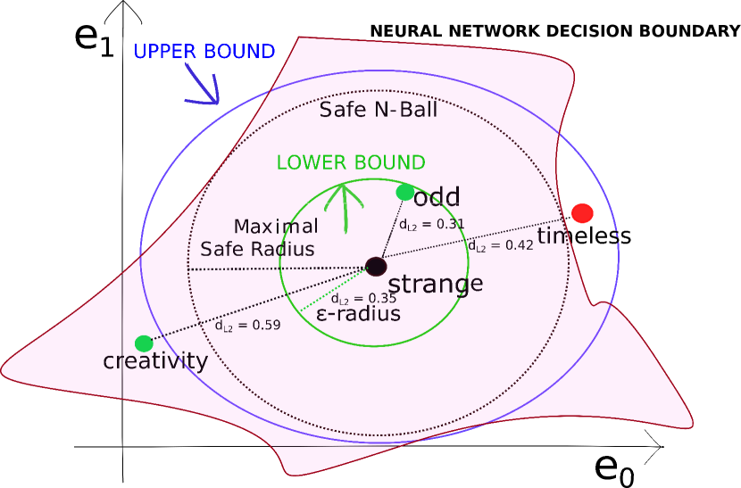
Figure 1: Illustration of the Maximal Safe Radius (MSR) and its upper and lower bounds. An upper bound of MSR is obtained by computing the distance of any perturbation resulting in a class change (blue ellipse) to the input text. A lower bound certifies that perturbations of the words contained within that radius are guaranteed to not change the classification decision (green ellipse). Both upper and lower bounds approximate the MSR (black ellipse). In this example the word strange can be safely substituted with odd. The word timeless is within upper and lower bound of the MSR, so our approach cannot guarantee it would not change the neural network prediction.

2.2 Upper Bound: Monte Carlo Tree Search

An upper bound for MSR is a perturbation of the text that is classified by the NN differently than the original text. In order to only consider perturbations that are syntactically coherent with the input text, we use filtering in conjunction with an adaptation of the Monte Carlo Tree Search (MCTS) algorithm Coulom (2007) to the NLP scenario (Figure 2). The algorithm takes as input a text, embeds it as a sequence of vectors $\bm{x}$, and builds a tree where at each iteration a set of indices $I$ identifies the words that have been modified so far: at the first level of the tree a single word is changed to manipulate the classification outcome, at the second two words are perturbed, with the former being the same word as for the parent vertex, and so on (i.e., for each vertex, $I$ contains the indices of the words that have been perturbed plus that of the current vertex). We allow only word for word substitutions. At each stage the procedure outputs all the successful attacks (i.e., perturbed texts that are classified by the neural network differently from the original text) that have been found until the terminating condition is satisfied (e.g., a fixed fraction out of the total number of vertices has been explored). Successful perturbations can be used as diagnostic information in cases where ground truth information is available. The algorithm explores the tree according to the UCT heuristic (Browne et al., 2012), where urgent vertices are identified by the perturbations that induce the largest drop in the neural network’s confidence. A detailed description of the resulting algorithm, which follows the classical algorithm Coulom (2007) while working directly with word embeddings, can be found in Appendix A.1. Perturbations are sampled by considering the $n$-closest replacements in the word’s neighbourhood: the distance between words is measured in the L₂ norm, while the number of substitutions per word is limited to a fixed constant (e.g., in our experiments this is either $1000$ or $10000$). In order to enforce the syntactic consistency of the replacements we consider part-of-speech tagging of each word based on its context. Then, we filter all the replacements found by MCTS to exclude those that are not of the same type, or from a type that will maintain the syntactic consistency of the perturbed text (e.g., a noun sometimes can be replaced by an adjective). To accomplish this task we use the Natural Language Toolkit (Bird et al., 2009). More details are provided in Appendix A.1.

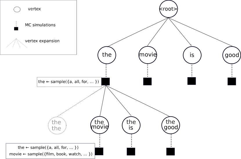
Figure 2: Structure of the tree after two iterations of the MCTS algorithm. Simulations of $1$-word substitutions are executed at each vertex on the first level to update the UCT statistics. The most urgent vertex is then expanded (e.g., word the) and several $2$-words substitutions are executed combining the word identified by the current vertex (e.g., word movie at the second level of the tree) and that of its parent, i.e., the. Redundant substitutions may be avoided (greyed out branch).

2.3 Lower Bound: Constraint Relaxation

A lower bound for $\texttt{MSR}(\mathbf{N},\bm{x})$ is a real number $\epsilon_{l}>0$ such that all texts in $\mathsf{Ball}(\bm{x},\epsilon_{l})$ are classified in the same class by $\mathbf{N}$. Note that, as $\texttt{MSR}(\mathbf{N},\bm{x})$ is defined in the embedding space, which is continuous, the perturbation space, $\mathsf{Ball}(\bm{x},\epsilon)$, contains meaningful texts as well as texts that are not syntactically or semantically meaningful. In order to compute $\epsilon_{l}$ we leverage constraint relaxation techniques developed for CNNs Boopathy et al. (2019) and LSTMs Ko et al. (2019), namely CNN-Cert and POPQORN. For an input text $\bm{x}$ and a hyper-box around $\mathsf{Ball}(\bm{x},\epsilon)$, these techniques find linear lower and upper bounds for the activation functions of each layer of the neural network and use these to propagate an over-approximation of the hyper-box through the network. $\epsilon_{l}$ is then computed as the largest real such that all the texts in $\mathsf{Ball}(\bm{x},\epsilon_{l})$ are in the same class, i.e., for all $\bm{x}^{\prime}\in\mathsf{Ball}(\bm{x},\epsilon_{l})$, $\arg\max_{i\in C}\mathbf{N}_{i}(\bm{x})=\arg\max_{i\in C}\mathbf{N}_{i}(\bm{x}^{\prime})$. Note that, as $\mathsf{Ball}(\bm{x},\epsilon_{l})$ contains only texts obtained by perturbing a subset of the words (those whose index is in $I$), to adapt CNN-Cert and POPQORN to our setting, we have to fix the dimensions of $\bm{x}$ corresponding to words not in $I$ and only propagate through the network intervals corresponding to words in $I.$

3 Experimental Results

	NEWS	SST	AG NEWS	IMDB
Inputs (Train, Test)	$22806,9793$	$117220,1821$	$120000,7000$	$25000,25000$
Output Classes	$7$	$2$	$4$	$2$
Average Input Length	$17\pm 2.17$	$17.058\pm 8.27$	$37.295\pm 9.943$	$230.8\pm 169.16$
Max Input Length	$88$	$52$	$136$	$2315$
Max Length Considered	$14$	$25$	$49$	$100$

Table 1: Datasets used for the experimental evaluation. We report the number of samples (training/test ratio as provided in the original works) and output classes, the average and maximum length of each input text before pre-processing and the maximum length considered in our experiments.

We use our framework to empirically evaluate the robustness of neural networks for sentiment analysis and news classification on typical CNN and LSTM architectures. While we quantify lower bounds of MSR for CNNs and LSTMs, respectively, with CNN-Cert and POPQORN tools, we implement the MCTS algorithm introduced in Section 2.2 to search for meaningful perturbations (i.e., upper bounds), regardless of the NN architecture employed. In particular, in Section 3.1 we consider robustness against single and multiple word substitutions and investigate implicit biases of LSTM architectures. In Section 3.2 we study the effect of embedding on robustness, while in Section 3.3 we employ our framework to perform saliency analysis of the most relevant words in a text.

Experimental Setup and Implementation

We have trained several vanilla CNN and LSTM models on datasets that differ in length of each input, number of target classes and difficulty of the learning task. All our experiments were conducted on a server equipped with two $24$ core Intel Xenon $6252$ processors and $256$GB of RAM^,. We consider the IMDB dataset (Maas et al., 2011), the Stanford Sentiment Treebank (SST) dataset (Socher et al., 2013), the AG News Corpus (Zhang et al., 2015) and the NEWS dataset (Vitale et al., 2012): details are in Table 1. In our experiments we consider different embeddings, and specifically both complex, probabilistically-constrained representations (GloVe and GloVeTwitter) trained on global word-word co-occurrence statistics from a corpus, as well as the simplified embedding provided by the Keras Python Deep Learning Library (referred to as Keras Custom) (Chollet et al., 2015), which allows one to fine tune the exact dimension of the vector space and only aims at minimizing the loss on the classification task. The resulting learned Keras Custom embedding does not capture complete word semantics, just their emotional polarity. More details are reported in Appendix A.3 and Table 4. For our experiments, we consider a $3$-layer CNN, where the first layer consists of bi-dimensional convolution with $150$ filters, each of size $3\times 3$, and a LSTM model with $256$ hidden neurons on each gate. We have trained more than $20$ architectures on the embeddings and datasets mentioned above. We note that, though other architectures might offer higher accuracy for sentence classification (Kim, 2014), this vanilla setup has been chosen intentionally not to be optimized for a specific task, thus allowing us to measure robustness of baseline models. Both CNNs and LSTMs predict the output with a $\mathsf{softmax}$ output layer, while the $\mathsf{categorical}$ $\mathsf{cross}$-$\mathsf{entropy}$ loss function is used during the optimization phase, which is performed with Adam Kingma and Ba (2014) algorithm (without early-stopping); further details are reported in Appendix A.3.

3.1 Robustness to Word Substitutions

For each combination of a neural network and embedding, we quantify the MSR against single and multiple word substitutions, meaning that the set of word indices $I$ (see Definition 1) consists of $1$ or more indices. Interestingly, our framework is able to prove that certain input texts and architectures are robust for any single-word substitution, that is, replacing a single word of the text (any word) with any other possible other word, and not necessarily with a synonym or a grammatically correct word, will not affect the classification outcome. Figure 3 shows that for CNN models equipped with Keras Custom embedding the (lower bound of the) MSR on some texts from the IMDB dataset is greater than the diameter of the embedding space.

	DIMENSION	LOWER BOUND
Keras	$5$	$0.278$
	$10$	$0.141$
	$25$	$0.023$
	$50$	$0.004$
	$100$	$0.002$
GloVe	$50$	$0.007$
	$100$	$0.002$
GloVeTwitter	$25$	$0.013$
	$50$	$0.008$
	$100$	$0.0$

Table 2: Comparison of lower bounds for single-word substitutions computed by CNN-Cert on the SST dataset. Values are averaged over $100$ input texts (approx. $2500$ measurements) and normalized by the embedding diameter (L₂-norm).

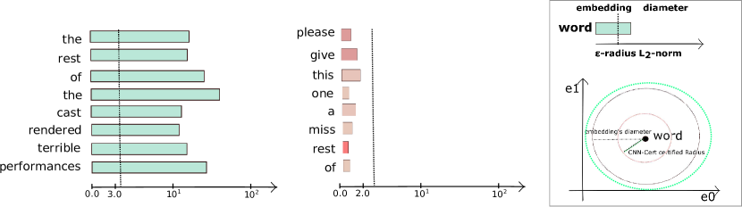
Figure 3: Lower bounds indicate classification invariance to any substitution when greater than the embedding diameter $\mathbf{d}$ (see diagram on the right and Section 2), here represented by the dotted vertical line. Left: Examples of words safe to any substitution (IMDB, Keras embedding $10d$, text no 2). Middle: Examples of words vulnerable to substitutions that may change the classification (IMDB, Keras embedding $5d$, text no 1).

To consider only perturbations that are semantically close and syntactically coherent with the input text, we employ the MCTS algorithm with filtering described in Section 2.2. An example of a successful perturbation is shown in Figure 4, where we illustrate the effectiveness of single-word substitutions on inputs that differ in the confidence of the neural network prediction. We note that even with simple tagging it is possible to identify perturbations where replacements are meaningful. For the first example in Figure 4 (top), the network changes the output class to World when the word China is substituted for U.S.. Although this substitution may be relevant to that particular class, nonetheless we note that the perturbed text is coherent and the main topic remains sci-tech. Furthermore, the classification changes also when the word exists is replaced with a plausible alternative misses, a perturbation that is neutral, i.e. not informative for any of the possible output classes. In the third sentence in Figure 4 (bottom), we note that replacing championship with wrestling makes the model output class World, where originally it was Sport, indicating that the model relies on a small number of key words to make its decision. We report a few additional examples of word replacements for a CNN model equipped with GloVe-50d embedding. Given as input the review ’this is art paying homage to art’ (from the SST dataset), when art is replaced by graffiti the network misclassifies the review (from positive to negative). Further, as mentioned earlier, the MCTS framework is capable of finding multiple word perturbations: considering the same setting as in the previous example, when in the review ’it’s not horrible just horribly mediocre’ the words horrible and horribly are replaced, respectively, with gratifying and decently, the review is classified as positive, while for the original sentence it was negative. Robustness results for high-dimensional embeddings are included in Table 3, where we report the trends of the average lower and upper bounds of MSR and the percentage of successful perturbations computed over $100$ texts (per dataset) for different architectures and embeddings. Further results are in Appendix A.3, including statistics on lower bounds (Tables 5, 6) and single and multiple word substitutions (Tables 7, 8).

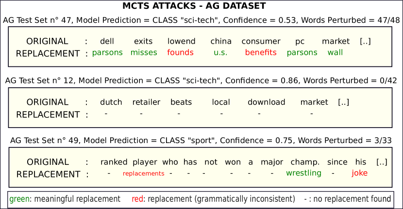
Figure 4: Single-word substitutions found with MCTS in conjunction with filtering. Grammatically consistent substitutions shown in green, inconsistent in red, a dash indicates that no substitution is found.

Single-Word Substitutions
EMBEDDING LOWER BOUND SUBSTITUTIONS UPPER BOUND % per text % per word IMDB Keras$50$d $0.055\pm 0.011$ $6.0$ $1.4$ $0.986$ GloVe$50$d $0.018\pm 0.007$ $39.7$ $5.1$ $0.951$ GloVeTwitter$50$d $0.02\pm 0.002$ $47.0$ $7.7$ $0.926$ AG News Keras$50$d $0.002\pm 0.001$ $50.0$ $15.6$ $0.852$ GloVe$50$d $0.005\pm 0.004$ $22.4$ $10.8$ $0.898$ GloVeTwitter$50$d $0.007\pm 0.001$ $21.4$ $6.6$ $0.937$ SST Keras$50$d $0.004\pm 0.001$ $52.2$ $19.9$ $0.813$ GloVe$50$d $0.007\pm 0.003$ $81.1$ $37.4$ $0.646$ GloVeTwitter$50$d $0.008\pm 0.004$ $78.1$ $36.3$ $0.653$ NEWS GloVe$50$d $0.001\pm 0.002$ $96.5$ $34.0$ $0.679$ GloVe$100$d $0.002\pm 0.002$ $89.7$ $29.1$ $0.727$ GloVeTwitter$50$d $0.001\pm 0.001$ $90.9$ $30.6$ $0.707$ GloVeTwitter$100$d $0.001\pm 0.001$ $89.7$ $27.7$ $0.739$

Table 3: Statistics on single-word substitutions averaged on $100$ input texts of each dataset. We report: the average lower bound of the MSR as measured with either CNN-Cert or POPQORN; the approximate ratio that given a word from a text we find a single-word substitution and the average number of words that substituted for a given word change the classification; the average upper bound computed as the distance between the original word and the closest substitution found by MCTS (when no successful perturbation is found we over-approximate the upper bound for that word with the diameter of the embedding). Values reported for lower bounds have been normalized by each embedding diameter (measurements in the L₂-norm).

CNNs vs. LTSMs

By comparing the average robustness assigned to each word, respectively, by CNN-Cert and POPQORN over all the experiments on a fixed dataset, it clearly emerges that recurrent models are less robust to perturbations that occur in very first words of a sentence; interestingly, CNNs do not suffer from this problem. A visual comparison is shown in Figure 6. The key difference is the structure of LSTMs compared to CNNs: while in LSTMs the first input word influences the successive layers, thus amplifying the manipulations, the output of a convolutional region is independent from any other of the same layer. On the other hand, both CNNs and LSTMs have in common an increased resilience to perturbations on texts that contain multiple polarized words, a trend that suggests that, independently of the architecture employed, robustness relies on a distributed representation of the content in a text (Figure 5).

Figure 5: Lower bound values for individual words obtained from POPQORN ($L_{2}$-norm), showing an increasing trend for consecutive words. (a) Two texts with padding (<unk> denotes an unknown token). (b) Texts with several words related to a specific output class (U.S. and entertainment, respectively).

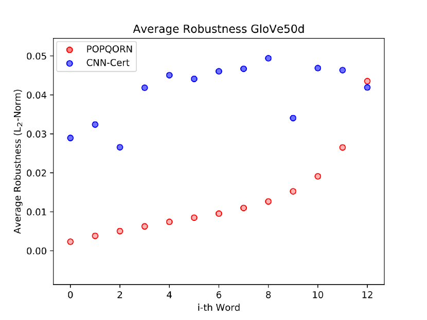
Figure 6: Robustness lower bound trends for successive input words for LSTMs (red dots) and CNNs (blue dots) on NEWS and AG News datasets.

3.2 Influence of the Embedding on Robustness

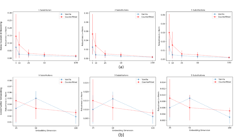
Figure 11: Comparison of robustness of vanilla vs. counter-fitted embeddings for an increasing number of dimensions and word substitutions on the AG News dataset. (a) Simple Keras Custom embeddings optimised for emotional polarity. (b) GloVeTwitter embeddings that encode more complex representations. Counter-fitted embeddings exhibit greater robustness on low-dimensional or simple embeddings. A reversed trend is observed on high-dimensional embeddings or more complex word representations. Values reported refer to measurements in the L_∞-norm.

As illustrated in Table 2 and in Figure 3, models that employ small embeddings are more robust to perturbations. On the contrary, robustness decreases, from one to two orders of magnitude, when words are mapped to high-dimensional spaces, a trend that is confirmed also by MCTS (see Appendix Table 8). This may be explained by the fact that adversarial perturbations are inherently related to the dimensionality of the input space (Carbone et al., 2020; Goodfellow et al., 2014). We also discover that models trained on longer inputs (e.g., IMDB) are more robust compared to those trained on shorter ones (e.g., SST): in long texts the decision made by the algorithm depends on multiple words that are evenly distributed across the input, while for shorter sequences the decision may depend on very few, polarized terms. From Table 3 we note that polarity-constrained embeddings (Keras) are more robust than those that are probabilistically-constrained (GloVe) on relatively large datasets (IMDB), whereas the opposite is true on smaller input dimensions: experiments suggest that models with embeddings that group together words closely related to a specific output class (e.g., positive words) are more robust, as opposed to models whose embeddings gather words together on a different principle (e.g., words that appear in the same context): intuitively, in the former case, words like good will be close to synonyms like better and nice, while in the latter words like good and bad, which often appear in the same context (think of the phrase ’the movie was good/bad’), will be closer in the embedding space. In the spirit of the analysis in (Baroni et al., 2014), we empirically measured whether robustness is affected by the nature of the embedding employed, that is, either prediction-based (i.e., embeddings that are trained alongside the classification task) or hybrid/count-based (e.g., GloVe, GloVeTwitter). By comparing the robustness of different embeddings and the distance between words that share the same polarity profile (e.g., positive vs. negative), we note that MSR is a particularly well suited robustness metric for prediction-based embeddings, with the distance between words serving as a reasonable estimator of word-to-word semantic similarity w.r.t. the classification task. On the other hand, for hybrid and count-based embeddings (e.g., GloVe), especially when words are represented as high-dimensional vectors, the distance between two words in the embedding space, when compressed into a single scalar, does not retain enough information to estimate the relevance of input variations. Therefore, in this scenario, an approach based solely on the MSR is limited by the choice of the distance function between words, and may lose its effectiveness unless additional factors such as context are considered. Further details of our evaluation are provided in Appendix A.3, Table 5 and Figure 11.

Counter-fitting

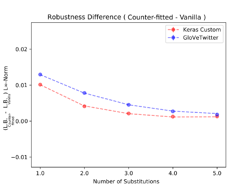
Figure 7: For an increasing number of substitutions per text we report the difference between MSR lower bounds of counter-fitted and vanilla embeddings (Keras and GloVeTwitter, $25$d) on the AG News Dataset.

To mitigate the issue of robustness in multi-class datasets characterized by short sequences, we have repeated the robustness measurements with counter-fitted (Mrkšić et al., 2016) embeddings, i.e., a method of injecting additional constraints for antonyms and synonyms into vector space representations in order to improve the vectors’ capability to encode semantic similarity. We observe that the estimated lower bound of MSR is in general increased for low-dimensional embeddings, up to twice the lower bound for non counter-fitted embeddings. This phenomenon is particularly relevant when Keras Custom $5$d and $10$d are employed, see Appendix A.3, Table 6. On the other hand, the benefits of counter-fitting are less pronounced for high-dimensional embeddings. The same pattern can be observed in Figure 7, where multiple-word substitutions per text are allowed. Further details can be found in Appendix A.3, Tables 6 and 8.

3.3 Interpretability of Sentiment Analysis via Saliency Maps

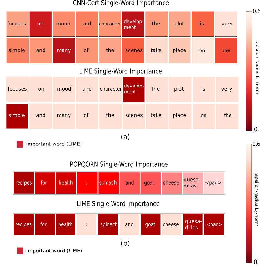
Figure 8: Interpretability comparison of our framework with LIME. (a) Saliency map produced with CNN-Cert (top) and LIME (bottom) on IMDB (GloVeTwitter $25$d embedding). (b) Saliency map produced with POPQORN (top) and LIME (bottom) on NEWS dataset (GloVe $100$d embedding).

We employ our framework to perform interpretablity analysis on a given text. For each word of a given text we compute the (lower bound of the) MSR and use this as a measure of its saliency, where small values of MSR indicate that minor perturbations of that word can have a significant influence on the classification outcome. We use the above measure to compute saliency maps for both CNNs and LSTMs, and compare our results with those obtained by LIME (Ribeiro et al., 2016), which assigns saliency to input features according to the best linear model that locally explains the decision boundary. Our method has the advantage of being able to account for non-linearities in the decision boundary that a local approach such as LIME cannot handle, albeit at a cost of higher computational complexity (a similar point was made in Blaas et al. (2020) for Gaussian processes). As a result, we are able to discover words that our framework views as important, but LIME does not, and vice versa. In Figure 8 we report two examples, one for an IMDB positive review (Figure 8 (a)) and another from the NEWS dataset classified using a LTSM (Figure 8 (b)). In Figure 8 (a) our approach finds that the word many is salient and perturbing it slightly can make the NN change the class of the review to negative. In contrast, LIME does not identify many as significant. In order to verify this result empirically, we run our MCTS algorithm (Section 2.2) and find that simply substituting many with worst changes the classification to ‘negative’. Similarly, for Figure 8 (b), where the input is assigned to class $5$ (health), perturbing the punctuation mark (:) may alter the classification, whereas LIME does not recognise its saliency.

4 Conclusions

We introduced a framework for evaluating robustness of NLP models against word substitutions. Through extensive experimental evaluation we demonstrated that our framework allows one to certify certain architectures against single word perturbations and illustrated how it can be employed for interpretability analysis. While we focus on perturbations that are syntactically coherent, we acknowledge that semantic similarity between phrases is a crucial aspect that nonetheless requires an approach which takes into account the context where substitutions happen: we will tackle this limitation in future. Furthermore, we will address robustness of more complex architectures, e.g., networks that exploit attention-based mechanisms  (Vaswani et al., 2017).

Acknowledgements

This project was partly funded by Innovate UK (reference 104814) and the ERC under the European Union’s Horizon 2020 research and innovation programme (grant agreement No. 834115). We thank the reviewers for their critical assessment and suggestions for improvement.

Appendix A Appendix

A.1 Monte Carlo Tree Search (MCTS)

We adapt the MCTS algorithm Browne et al. (2012) to the NLP classification setting with word embedding, which we report here for completeness as Algorithm 1. The algorithm explores modifications to the original text by substituting one word at the time with nearest neighbour alternatives. It takes as input: text, expressed as a list of $T$ words; $\mathbf{N}$, the neural network as introduced in Section 2; $\mathcal{E}$, an embedding; sims, an integer specifying the number of Monte Carlo samplings at each step; and $\alpha$, a real-valued meta-parameter specifying the exploration/exploitation trade-off for vertices that can be further expanded. The salient steps of the MCTS procedure are:

• Select: the most promising vertex to explore is chosen to be expanded (Line 15) according to the standard UCT heuristic:
  $\dfrac{Q(v)}{N(v)}+\alpha\sqrt{\dfrac{2lnN(v^{\prime})}{N(v)}}$, where $v$ and $v^{\prime}$ are respectively the selected vertex and its parent; $\alpha$ is a meta-parameter that balances exploration-exploitation trade-off; $N()$ represents the number of times a vertex has been visited; and $Q()$ measures the neural network confidence drop, averaged over the Monte Carlo simulations for that specific vertex.

• Expand: the tree is expanded with $T$ new vertices, one for each word in the input text (avoiding repetitions). A vertex at index $t\in\{1,...T\}$ and depth $n>0$ represents the strategy of perturbing the $t$-th input word, plus all the words whose indices have been stored in the parents of the vertex itself, up to the root.

• Simulate: simulations are run from the current position in the tree to estimate how the neural network behaves against the perturbations sampled at that stage (Line 26). If one of the word substitutions induced by the simulation makes the network change the classification, a successful substitution is found and added to the results, while the value $Q$ of the current vertex is updated. Many heuristics can be considered at this stage, for example the average drop in the confidence of the network over all the simulations. We have found that the average drop is not a good measure of how the robustness of the network drops when some specific words are replaced, since for a high number of simulations a perturbation that is effective might pass unnoticed. We thus work with the maximum drop over all the simulations, which works slightly better in this scenario (Line 30).

• Backpropagate: the reward received is back-propagated to the vertices visited during selection and expansion to update their UCT statistics. It is known that, when UCT is employed (Browne et al., 2012; Kocsis and Szepesvári, 2006), MCTS guarantees that the probability of selecting a sub-optimal perturbation tends to zero at a polynomial rate when the number of games grows to infinity (i.e., it is guaranteed to find a discrete perturbation, if it exists).

Algorithm 1 Monte Carlo Tree Search with UCT heuristic

1:procedure MCTS($text,\ \mathbf{N},\ \mathcal{E},\ sims,\ \alpha$)

2:     $t\leftarrow\arg\max_{i\in C}\mathbf{N}_{i}(\mathcal{E}(text))$ $\triangleright$ Store the unperturbed network output, ref. Section2

3:     $Tree\leftarrow createTree(text,\ c,\ \mathbf{N})$ $\triangleright$ Create the initial tree

4:     $root\leftarrow getRoot(Tree)$ $\triangleright$ Store the initial vertex

5:     $P\leftarrow[\ ]$ $\triangleright$ List of final perturbations

6:     while $terminate(Tree)\not=True$ do $\triangleright$ Loop over the MCTS steps

7:         $v\leftarrow$SELECT$(Tree,\ \alpha)$

8:         $C\leftarrow$EXPAND$(v,\ text)$

9:         $P.insert($SIMULATE$(C,\ text,\ sims,\ \mathbf{N},\ \mathcal{E},\ t))$

10:         BACKPROPAGATE$(v,root)$      

11:     return $P$

12:

13:procedure Select($Tree,\ \alpha$)

14:     $L\leftarrow getLeaves(Tree)$

15:     return $\operatorname*{argmax}_{v\in L}\dfrac{Q(v)}{N(v)}+\alpha\sqrt{\dfrac{2lnN(v^{\prime})}{N(v)}}$ $\triangleright$ UCT best leaf

16:

17:procedure Expand($v,\ text$)

18:     for $i=0$, $i<length(text)$, $i{+}{+}$ do

19:         $v.expand(i)$ $\triangleright$ Create v’s i-th child      

20:     return $getChildren(v)$ $\triangleright$ Return the expanded children

21:

22:procedure Simulate($C,\ text,\ sims,\ \mathbf{N},\ \mathcal{E},\ t$)

23:     $Perturbations\leftarrow[\ ]$

24:     for $c\in C$ do

25:         for $i=0$, $i<sims$, $i{+}{+}$ do

26:              $text^{\prime}\leftarrow samplePerturbation(text,\ c)$ $\triangleright$ Ref. Figure 9

27:              $x\leftarrow\mathcal{E}(text);\ x_{i}^{\prime}\leftarrow\mathcal{E}(text^{\prime})$ $\triangleright$ Embed inputs

28:              if $\mathbf{N}(x_{i}^{\prime})\not=\mathbf{N}(x)$ then $\triangleright$ The output class changes

29:                  $Perturbations.append(text^{\prime})$                        

30:         $Q(c)$ = $max_{i\in sims}(\mathbf{N}_{t}(x)-\mathbf{N}_{t}(x^{\prime}_{i}))$ $\triangleright$ Update vertex heuristic      

31:     return $Perturbations$

32:

33:procedure Backpropagate($v,\ root$) $\triangleright$ Propagate UCT update

34:     while $v\not=root$ do

35:         $updateUCT(v)$

36:         $v\leftarrow getParent(v)$      

For our implementation we adopted $\textit{sims}=1000$ and $\alpha=0.5$. Tables 8 and 7 give details of MCTS experiments with single and multiple word substitutions.

MCTS Word Substitution Strategies

We consider two refinements of MCTS: weighting the replacement words by importance and filtering to ensure syntactic/semantic coherence of the input text. The importance score of a word substitution is inversely proportional to its distance from the original word, e.g., $pickup(w\leftarrow w^{\prime})=\dfrac{1}{\absolutevalue{U}-1}(\dfrac{\sum_{u\in U\setminus\{w^{\prime}\}}d(w,u)}{\sum_{u\in U}d(w,u)})$, where $w,w^{\prime}$ are respectively the original and perturbed words, $d()$ is an $L^{p}$ norm of choice and $U$ a neighbourhood of $w$, whose cardinality, which must be greater than $1$, is denoted with $\absolutevalue{U}$ (as shown in Figure 9). We can further filter words in the neighborhood such that only synonyms/antonyms are selected, thus guaranteeing that a word is replaced by a meaningful substitution; more details are provided in Section 2.2. While in this work we use a relatively simple method to find replacements that are syntactically coherent with the input text, more complex methods are available that try also to enforce semantic consistency (Navigli, 2009; Ling et al., 2015; Trask et al., 2015), despite this problem is known to be much harder and we reserve this for future works.

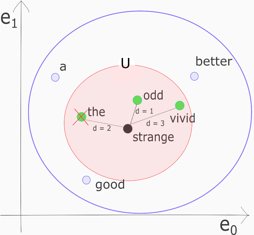
Figure 9: Substitutions are selected either randomly or according to a score calculated as a function of the distance from the original word. The sampling region (red circle) is a finite fraction of the embedding space (blue circle). Selected candidates can be filtered to enforce semantic and syntactic constraints. Word the has been filtered out because it is not grammatically consistent with the original word strange, while words good, better and a are filtered out as they lie outside the neighborhood of the original word.

A.2 Experimental Setup

The network architectures that have been employed in this work are shown in Figure 10, while the embeddings are summarised in Table 4. More details of both the embeddings and the architectures employed are provided in the main paper, Section 3.

A.3 Additional Robustness Results

In the remainder of this section we present additional experimental results of our robustness evaluation. More specifically, we show the trends of upper and lower bounds for different datasets (Tables 5, 6, 7 and 8); include robustness results against multiple substitutions; and perform robustness comparison with counter-fitted models (Figure 11).

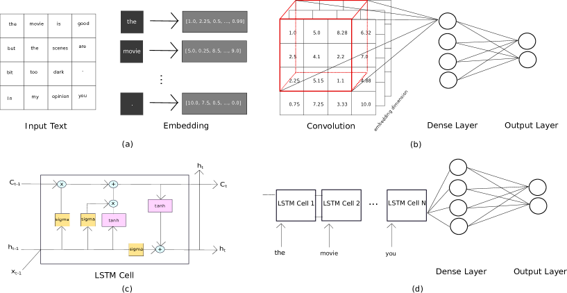
Figure 10: Architecture of CNN and LSTM vanilla models used in this work. (a) Embedding of input words as vectors of real numbers that are passed as input to a network model that outputs the class to which a text belongs (shown here with two outputs, e.g., a positive, negative review of a movie). (b) Convolutional network (CNN) model. (d) LSTM network model. (c) A single LSTM cell in detail.

Embeddings
DIM WORDS DIAMETER DIAMETER (raw) Keras $5$ $177175$ $2.236$ $1.144$ $10$ $88587$ $3.162$ $0.957$ $25$ 88587 $5$ $0.763$ $50$ $88587$ $7.07$ $0.664$ $100$ $88587$ $10$ $0.612$ GloVe $50$ $400003$ $7.071$ $10.918$ $100$ $400003$ $10$ $8.133$ GloVeTwitter $25$ $1193517$ $5$ $21.15$ $50$ $1193517$ $7.071$ $13.947$ $100$ $1193517$ $10$ $13.058$

Table 4: Embeddings used for the experimental evaluation: we report the number of dimensions, the number of words in each vocabulary and the maximum distance between the two farthest words, namely the diameter (both after normalization of the input vectors and the raw value, expressed in the L₂-norm). After normalization, an embedding of dimension $d$ will have a diameter equal to $\sqrt{d}$, as a consequence of scaling to $1$ the difference between maximum and minimum values for any dimension of the input.

IMDB
DIMENSION ACCURACY LOWER BOUND Keras $5$ $0.789$ $1.358\pm 0.604$ $10$ $0.788$ $2.134\pm 1.257$ $25$ $0.78$ $1.234\pm 2.062$ $50$ $0.78$ $0.394\pm 0.079$ $100$ $0.778$ $0.31\pm 0.041$ GloVe $50$ $0.758$ $0.133\pm 0.054$ $100$ $0.783$ $0.127\pm 0.055$ GloVeTwitter $25$ $0.739$ $0.168\pm 0.093$ $50$ $0.752$ $0.143\pm 0.02$ $100$ $0.77$ $0.177\pm 0.057$
Stanford Sentiment Treebank (SST)
DIMENSION ACCURACY LOWER BOUND Keras $5$ $0.75$ $0.623\pm 0.28$ $10$ $0.756$ $0.449\pm 0.283$ $25$ $0.757$ $0.116\pm 0.14$ $50$ $0.811$ $0.029\pm 0.012$ $100$ $0.818$ $0.023\pm 0.006$ GloVe $50$ $0.824$ $0.053\pm 0.023$ $100$ $0.833$ $0.028\pm 0.015$ GloVeTwitter $25$ $0.763$ $0.065\pm 0.023$ $50$ $0.826$ $0.059\pm 0.031$ $100$ $0.823$ $0.0\pm 0.0$ (NaN)
NEWS Dataset
DIMENSION ACCURACY LOWER BOUND GloVe $50$ $0.625$ $0.013\pm 0.015$ $100$ $0.7$ $0.018\pm 0.017$ GloVeTwitter $50$ $0.627$ $0.009\pm 0.006$ $100$ $0.716$ $0.008\pm 0.009$

Table 5: Lower bound results for single-word substitutions as found by CNN-Cert and POPQORN, respectively, on the IMDB, SST and NEWS datasets. Values reported refer to measurements in the L₂-norm.

AG News Results: Single Word Substitution
DIAMETER ACCURACY LOWER BOUND Vanilla Counter-fitted Vanilla Counter-fitted Keras $5$ $0.414$ $0.464$ $0.072\pm 0.066$ $0.145\pm 0.147$ $10$ $0.491$ $0.505$ $0.026\pm 0.025$ $0.088\pm 0.087$ $25$ $0.585$ $0.597$ $0.022\pm 0.025$ $0.032\pm 0.026$ $50$ $0.692$ $0.751$ $0.015\pm 0.009$ $0.024\pm 0.015$ $100$ $0.779$ $0.807$ $0.011\pm 0.007$ $0.015\pm 0.009$ GloVe $50$ $0.892$ $0.879$ $0.04\pm 0.028$ $0.043\pm 0.03$ $100$ $0.901$ $0.887$ $0.027\pm 0.018$ $0.0\pm 0.0$ (NaN) GloVeTwitter $25$ $0.848$ $0.846$ $0.033\pm 0.025$ $0.046\pm 0.036$ $50$ $0.877$ $0.866$ $0.05\pm 0.012$ $0.033\pm 0.018$ $100$ $0.833$ $0.883$ $0.019\pm 0.012$ $0.026\pm 0.005$
AG News Results: Multiple Words Substitutions
DIAMETER L.B. 2 SUBSTITUTIONS L.B. 3 SUBSTITUTIONS Vanilla Counter-fitted Vanilla Counter-fitted Keras $5$ $0.029\pm 0.024$ $0.065\pm 0.059$ $0.025\pm 0.017$ $0.054\pm 0.044$ $10$ $0.013\pm 0.012$ $0.043\pm 0.042$ $0.008\pm 0.008$ $0.028\pm 0.028$ $25$ $0.011\pm 0.008$ $0.015\pm 0.012$ $0.007\pm 0.006$ $0.01\pm 0.008$ $50$ $0.007\pm 0.004$ $0.012\pm 0.007$ $0.005\pm 0.003$ $0.008\pm 0.005$ $100$ $0.006\pm 0.004$ $0.006\pm 0.004$ $0.003\pm 0.003$ $0.003\pm 0.002$ GloVe $50$ $0.02\pm 0.013$ $0.02\pm 0.014$ $0.013\pm 0.009$ $0.016\pm 0.01$ $100$ $0.015\pm 0.007$ $0.0\pm 0.0$ (NaN) $0.01\pm 0.006$ $0.0\pm 0.0$ (NaN) GloVeTwitter $25$ $0.014\pm 0.011$ $0.023\pm 0.017$ $0.01\pm 0.008$ $0.0015\pm 0.012$ $50$ $0.024\pm 0.005$ $0.015\pm 0.009$ $0.016\pm 0.004$ $0.011\pm 0.007$ $100$ $0.009\pm 0.006$ $0.013\pm 0.002$ $0.006\pm 0.004$ $0.008\pm 0.002$
DIAMETER L.B. 4 SUBSTITUTIONS L.B. 5 SUBSTITUTIONS Vanilla Counter-fitted Vanilla Counter-fitted Keras $5$ $0.018\pm 0.012$ $0.035\pm 0.028$ $0.014\pm 0.009$ $0.03\pm 0.021$ $10$ $0.006\pm 0.005$ $0.02\pm 0.019$ $0.005\pm 0.004$ $0.016\pm 0.015$ $25$ $0.005\pm 0.004$ $0.007\pm 0.006$ $0.004\pm 0.003$ $0.006\pm 0.004$ $50$ $0.003\pm 0.002$ $0.005\pm 0.002$ $0.003\pm 0.002$ $0.005\pm 0.003$ $100$ $0.003\pm 0.002$ $0.003\pm 0.002$ $0.002\pm 0.001$ $0.002\pm 0.001$ GloVe $50$ $0.009\pm 0.006$ $0.01\pm 0.006$ $0.008\pm 0.005$ $0.008\pm 0.006$ $100$ $0.007\pm 0.004$ $0.0\pm 0.0$ (NaN) $0.005\pm 0.003$ $0.0\pm 0.0$ (NaN) GloVeTwitter $25$ $0.007\pm 0.005$ $0.011\pm 0.008$ $0.006\pm 0.004$ $0.009\pm 0.006$ $50$ $0.008\pm 0.004$ $0.008\pm 0.006$ $0.009\pm 0.001$ $0.006\pm 0.004$ $100$ $0.004\pm 0.003$ $0.006\pm 0.001$ $0.003\pm 0.002$ $0.005\pm 0.001$

Table 6: Lower bound results for single (top) and multiple word (middle and bottom) substitutions, comparing vanilla and counter-fitted models. Robustness of counter-fitted models is superior to the vanilla counterpart, except for high-dimensional embeddings such as GloVe $100$d, where it has not been possible to obtain a bound for the counter-fitted embedding due to computational constraints (nonetheless the counterpart lower bound is close to zero). Values reported refer to measurements in the L_∞-norm.

MCTS Results
EMBEDDING EXEC TIME [s] SUB. (% per-text) SUB. (% per-word) UB IMDB Keras$50$d $29.52$ $6.0$ $1.4$ $0.41\pm 0.04$ GloVe$50$d $39.61$ $39.7$ $5.1$ $0.39\pm 0.016$ GloVeTwitter$50$d $54.1$ $47.0$ $7.7$ $0.329\pm 0.015$ AG NEWS Keras$50$d $21.09$ $50.0$ $15.6$ $0.396\pm 0.02$ GloVe$50$d $19.25$ $22.4$ $10.8$ $0.438\pm 0.042$ GloVeTwitter$50$d $17.75$ $21.4$ $6.6$ $0.336\pm 0.019$ SST Keras$50$d $8.36$ $52.2$ $19.9$ $0.444\pm 0.077$ GloVe$50$d $11.94$ $81.1$ $37.4$ $0.385\pm 0.024$ GloVeTwitter$50$d $11.96$ $78.1$ $36.3$ $0.329\pm 0.024$ NEWS GloVe$50$d $75.76$ $96.5$ $34.0$ $0.405\pm 0.045$ GloVe$100$d $79.31$ $89.7$ $29.1$ $0.442\pm 0.042$ GloVeTwitter$50$d $77.74$ $90.9$ $30.6$ $0.314\pm 0.033$ GloVeTwitter$100$d $81.29$ $89.7$ $27.7$ $0.417\pm 0.042$

Table 7: Upper bound results for single-word substitutions as found by MCTS. We report: the average execution time for each experiment; the percentage of texts for which we have found at least one successful single-word substitution (which results in a class change) and the approximate ratio that selecting randomly 1 word from a text we find a replacement that is successful; the distance to the closest meaningful perturbation to the original word found, namely an upper bound (differently from Table 3 and for completeness, here values are reported only considering the values for those words where the perturbations were successful). Values reported refer to measurements in the L₂-norm.

MCTS Multiple Substitutions
EMBEDDING 2 SUBSTITUTIONS 3 SUBSTITUTIONS 4 SUBSTITUTIONS % per-text % per-word % per-text % per-word % per-text % per-word IMDB Keras$50$d $8.5$ $5.0$ $13.4$ $5.9$ $18.2$ $6.6$ GloVe$50$d $43.8$ $17.7$ $52.0$ $21.6$ $57.5$ $24.5$ GloVeTwitter$50$d $44.1$ $18.3$ $49.3$ $23.0$ $57.1$ $26.4$ AG NEWS Keras$50$d $68.1$ $27.5$ $72.7$ $38.3$ $83.3$ $47.9$ GloVe$50$d $31.4$ $15.8$ $33.7$ $16.8$ $37.0$ $19.7$ GloVeTwitter$50$d $23.8$ $12.5$ $23.8$ $15.3$ $38.0$ $18.4$ SST Keras$50$d $64.8$ $33.0$ $74.7$ $40.2$ $78.0$ $48.7$ GloVe$50$d $89.4$ $58.0$ $96.4$ $70.8$ $97.6$ $76.5$ GloVeTwitter$50$d $88.3$ $57.8$ $94.1$ $69.1$ $95.3$ $74.9$ NEWS GloVe$50$d $98.8$ $55.4$ $97.3$ $62.5$ $97.3$ $68.6$ GloVe$100$d $100.0$ $46.8$ $95.0$ $68.0$ $96.0$ $65.2$ GloVeTwitter$50$d $94.5$ $50.5$ $97.5$ $63.0$ $97.5$ $71.9$ GloVeTwitter$100$d $92.7$ $49.9$ $98.1$ $58.2$ $98.3$ $65.3$

Table 8: Upper bound results for multiple-word substitutions as found by MCTS. We report the percentage of texts for which we have found at least a single-word substitution and the approximate ratio that selecting randomly $k$ words from a text (where $k$ is the number of substitutions allowed) we find a replacement that is successful. We do not report the average execution times as they are (roughly) the same as in Table 7. Values reported refer to measurements in the L₂-norm. For more than $1$ substitution, values reported are an estimate on several random replacements, as it quickly becomes prohibitive to cover all the possible multiple-word combinations.

References

- Alzantot et al. (2018) Moustafa Alzantot, Yash Sharma, Ahmed Elgohary, Bo-Jhang Ho, Mani Srivastava, and Kai-Wei Chang. 2018. Generating natural language adversarial examples. arXiv preprint arXiv:1804.07998.
- Arras et al. (2016) Leila Arras, Franziska Horn, Grégoire Montavon, Klaus-Robert Müller, and Wojciech Samek. 2016. Explaining predictions of non-linear classifiers in nlp. arXiv preprint arXiv:1606.07298.
- Baroni et al. (2014) Marco Baroni, Georgiana Dinu, and Germán Kruszewski. 2014. Don’t count, predict! a systematic comparison of context-counting vs. context-predicting semantic vectors. In Proceedings of the 52nd Annual Meeting of the Association for Computational Linguistics (Volume 1: Long Papers), pages 238–247, Baltimore, Maryland. Association for Computational Linguistics.
- Belinkov and Bisk (2018) Yonatan Belinkov and Yonatan Bisk. 2018. Synthetic and natural noise both break neural machine translation. In International Conference on Learning Representations.
- Biggio et al. (2013) Battista Biggio, Igino Corona, Davide Maiorca, Blaine Nelson, Nedim Šrndić, Pavel Laskov, Giorgio Giacinto, and Fabio Roli. 2013. Evasion attacks against machine learning at test time. In Joint European conference on machine learning and knowledge discovery in databases, pages 387–402. Springer.
- Biggio and Roli (2018) Battista Biggio and Fabio Roli. 2018. Wild patterns: Ten years after the rise of adversarial machine learning. Pattern Recognition, 84:317–331.
- Bird et al. (2009) Steven Bird, Ewan Klein, and Edward Loper. 2009. Natural language processing with Python: analyzing text with the natural language toolkit. ” O’Reilly Media, Inc.”.
- Blaas et al. (2020) Arno Blaas, Andrea Patane, Luca Laurenti, Luca Cardelli, Marta Kwiatkowska, and Stephen Roberts. 2020. Adversarial robustness guarantees for classification with gaussian processes. In International Conference on Artificial Intelligence and Statistics, pages 3372–3382.
- Boopathy et al. (2019) Akhilan Boopathy, Tsui-Wei Weng, Pin-Yu Chen, Sijia Liu, and Luca Daniel. 2019. Cnn-cert: An efficient framework for certifying robustness of convolutional neural networks. In Proceedings of the AAAI Conference on Artificial Intelligence, volume 33, pages 3240–3247.
- Browne et al. (2012) Cameron B Browne, Edward Powley, Daniel Whitehouse, Simon M Lucas, Peter I Cowling, Philipp Rohlfshagen, Stephen Tavener, Diego Perez, Spyridon Samothrakis, and Simon Colton. 2012. A survey of monte carlo tree search methods. IEEE Transactions on Computational Intelligence and AI in games, 4(1):1–43.
- Carbone et al. (2020) Ginevra Carbone, Matthew Wicker, Luca Laurenti, Andrea Patane, Luca Bortolussi, and Guido Sanguinetti. 2020. Robustness of bayesian neural networks to gradient-based attacks. arXiv preprint arXiv:2002.04359.
- Cheng et al. (2017) Chih-Hong Cheng, Georg Nührenberg, and Harald Ruess. 2017. Maximum resilience of artificial neural networks. In Automated Technology for Verification and Analysis, pages 251–268, Cham. Springer International Publishing.
- Cheng et al. (2018) Minhao Cheng, Jinfeng Yi, Huan Zhang, Pin-Yu Chen, and Cho-Jui Hsieh. 2018. Seq2sick: Evaluating the robustness of sequence-to-sequence models with adversarial examples. arXiv preprint arXiv:1803.01128.
- Chollet et al. (2015) François Chollet et al. 2015. keras.
- Chorowski et al. (2015) Jan K Chorowski, Dzmitry Bahdanau, Dmitriy Serdyuk, Kyunghyun Cho, and Yoshua Bengio. 2015. Attention-based models for speech recognition. In Advances in neural information processing systems, pages 577–585.
- Coulom (2007) Rémi Coulom. 2007. Efficient selectivity and backup operators in monte-carlo tree search. In Computers and Games, pages 72–83, Berlin, Heidelberg. Springer Berlin Heidelberg.
- Devlin et al. (2018) Jacob Devlin, Ming-Wei Chang, Kenton Lee, and Kristina Toutanova. 2018. Bert: Pre-training of deep bidirectional transformers for language understanding. arXiv preprint arXiv:1810.04805.
- Dutta et al. (2018) Souradeep Dutta, Susmit Jha, Sriram Sankaranarayanan, and Ashish Tiwari. 2018. Output range analysis for deep feedforward neural networks. In NASA Formal Methods, pages 121–138.
- Ebrahimi et al. (2018) Javid Ebrahimi, Anyi Rao, Daniel Lowd, and Dejing Dou. 2018. Hotflip: White-box adversarial examples for text classification. In Proceedings of the 56th Annual Meeting of the Association for Computational Linguistics (Volume 2: Short Papers), pages 31–36.
- Ettinger et al. (2017) Allyson Ettinger, Sudha Rao, Hal Daumé III, and Emily M Bender. 2017. Towards linguistically generalizable nlp systems: A workshop and shared task. In Proceedings of the First Workshop on Building Linguistically Generalizable NLP Systems, pages 1–10.
- Gao et al. (2018) Ji Gao, Jack Lanchantin, Mary Lou Soffa, and Yanjun Qi. 2018. Black-box generation of adversarial text sequences to evade deep learning classifiers. In 2018 IEEE Security and Privacy Workshops (SPW), pages 50–56. IEEE.
- Goldberg and Levy (2014) Yoav Goldberg and Omer Levy. 2014. word2vec explained: deriving mikolov et al.’s negative-sampling word-embedding method. arXiv preprint arXiv:1402.3722.
- Goodfellow et al. (2014) Ian J Goodfellow, Jonathon Shlens, and Christian Szegedy. 2014. Explaining and harnessing adversarial examples. arXiv preprint arXiv:1412.6572.
- Huang et al. (2019) Po-Sen Huang, Robert Stanforth, Johannes Welbl, Chris Dyer, Dani Yogatama, Sven Gowal, Krishnamurthy Dvijotham, and Pushmeet Kohli. 2019. Achieving verified robustness to symbol substitutions via interval bound propagation. In Proceedings of the 2019 Conference on Empirical Methods in Natural Language Processing and the 9th International Joint Conference on Natural Language Processing (EMNLP-IJCNLP), pages 4074–4084.
- Huang et al. (2017) Xiaowei Huang, Marta Kwiatkowska, Sen Wang, and Min Wu. 2017. Safety verification of deep neural networks. In International Conference on Computer Aided Verification, pages 3–29. Springer.
- Iyyer et al. (2018) Mohit Iyyer, John Wieting, Kevin Gimpel, and Luke Zettlemoyer. 2018. Adversarial example generation with syntactically controlled paraphrase networks. In Proceedings of the 2018 Conference of the North American Chapter of the Association for Computational Linguistics: Human Language Technologies, Volume 1 (Long Papers), pages 1875–1885.
- Jia and Liang (2017) Robin Jia and Percy Liang. 2017. Adversarial examples for evaluating reading comprehension systems. In Proceedings of the 2017 Conference on Empirical Methods in Natural Language Processing, pages 2021–2031.
- Jia et al. (2019) Robin Jia, Aditi Raghunathan, Kerem Göksel, and Percy Liang. 2019. Certified robustness to adversarial word substitutions. In Proceedings of the 2019 Conference on Empirical Methods in Natural Language Processing and the 9th International Joint Conference on Natural Language Processing (EMNLP-IJCNLP), pages 4120–4133.
- Jia et al. (2018) Ye Jia, Yu Zhang, Ron Weiss, Quan Wang, Jonathan Shen, Fei Ren, Patrick Nguyen, Ruoming Pang, Ignacio Lopez Moreno, Yonghui Wu, et al. 2018. Transfer learning from speaker verification to multispeaker text-to-speech synthesis. In Advances in neural information processing systems, pages 4480–4490.
- Katz et al. (2017) Guy Katz, Clark Barrett, David L Dill, Kyle Julian, and Mykel J Kochenderfer. 2017. Reluplex: An efficient smt solver for verifying deep neural networks. In International Conference on Computer Aided Verification, pages 97–117. Springer.
- Katz et al. (2019) Guy Katz, Derek A Huang, Duligur Ibeling, Kyle Julian, Christopher Lazarus, Rachel Lim, Parth Shah, Shantanu Thakoor, Haoze Wu, Aleksandar Zeljić, et al. 2019. The marabou framework for verification and analysis of deep neural networks. In International Conference on Computer Aided Verification, pages 443–452. Springer.
- Kim (2014) Yoon Kim. 2014. Convolutional neural networks for sentence classification. In Proceedings of the 2014 Conference on Empirical Methods in Natural Language Processing (EMNLP), pages 1746–1751, Doha, Qatar. Association for Computational Linguistics.
- Kingma and Ba (2014) Diederik P Kingma and Jimmy Ba. 2014. Adam: A method for stochastic optimization. arXiv preprint arXiv:1412.6980.
- Ko et al. (2019) Ching-Yun Ko, Zhaoyang Lyu, Lily Weng, Luca Daniel, Ngai Wong, and Dahua Lin. 2019. POPQORN: Quantifying robustness of recurrent neural networks. In International Conference on Machine Learning, pages 3468–3477.
- Kocsis and Szepesvári (2006) Levente Kocsis and Csaba Szepesvári. 2006. Bandit based monte-carlo planning. In European conference on Machine Learning, pages 282–293. Springer.
- Liang et al. (2017) Bin Liang, Hongcheng Li, Miaoqiang Su, Pan Bian, Xirong Li, and Wenchang Shi. 2017. Deep text classification can be fooled. arXiv preprint arXiv:1704.08006.
- Ling et al. (2015) Wang Ling, Chris Dyer, Alan W Black, and Isabel Trancoso. 2015. Two/too simple adaptations of word2vec for syntax problems. In Proceedings of the 2015 Conference of the North American Chapter of the Association for Computational Linguistics: Human Language Technologies, pages 1299–1304.
- Maas et al. (2011) Andrew L Maas, Raymond E Daly, Peter T Pham, Dan Huang, Andrew Y Ng, and Christopher Potts. 2011. Learning word vectors for sentiment analysis. In Proceedings of the 49th annual meeting of the association for computational linguistics: Human language technologies-volume 1, pages 142–150. Association for Computational Linguistics.
- Mrkšić et al. (2016) Nikola Mrkšić, Diarmuid O Séaghdha, Blaise Thomson, Milica Gašić, Lina Rojas-Barahona, Pei-Hao Su, David Vandyke, Tsung-Hsien Wen, and Steve Young. 2016. Counter-fitting word vectors to linguistic constraints. arXiv preprint arXiv:1603.00892.
- Navigli (2009) Roberto Navigli. 2009. Word sense disambiguation: A survey. ACM computing surveys (CSUR), 41(2):1–69.
- Pennington et al. (2014) Jeffrey Pennington, Richard Socher, and Christopher Manning. 2014. Glove: Global vectors for word representation. In Proceedings of the 2014 conference on empirical methods in natural language processing (EMNLP), pages 1532–1543.
- Ribeiro et al. (2016) Marco Tulio Ribeiro, Sameer Singh, and Carlos Guestrin. 2016. ”why should I trust you?”: Explaining the predictions of any classifier. In Proceedings of the 22nd ACM SIGKDD International Conference on Knowledge Discovery and Data Mining, San Francisco, CA, USA, August 13-17, 2016, pages 1135–1144.
- Ribeiro et al. (2018) Marco Tulio Ribeiro, Sameer Singh, and Carlos Guestrin. 2018. Semantically equivalent adversarial rules for debugging nlp models. In Proceedings of the 56th Annual Meeting of the Association for Computational Linguistics (Volume 1: Long Papers), pages 856–865.
- Ruan et al. (2018) Wenjie Ruan, Xiaowei Huang, and Marta Kwiatkowska. 2018. Reachability analysis of deep neural networks with provable guarantees. In Proceedings of the 27th International Joint Conference on Artificial Intelligence, pages 2651–2659. AAAI Press.
- Socher et al. (2013) Richard Socher, Alex Perelygin, Jean Wu, Jason Chuang, Christopher D Manning, Andrew Y Ng, and Christopher Potts. 2013. Recursive deep models for semantic compositionality over a sentiment treebank. In Proceedings of the 2013 conference on empirical methods in natural language processing, pages 1631–1642.
- Szegedy et al. (2014) Christian Szegedy, Wojciech Zaremba, Ilya Sutskever, Joan Bruna, Dumitru Erhan, Ian Goodfellow, and Rob Fergus. 2014. Intriguing properties of neural networks. In International Conference on Learning Representations.
- Trask et al. (2015) Andrew Trask, Phil Michalak, and John Liu. 2015. sense2vec-a fast and accurate method for word sense disambiguation in neural word embeddings. arXiv preprint arXiv:1511.06388.
- Vaswani et al. (2017) Ashish Vaswani, Noam Shazeer, Niki Parmar, Jakob Uszkoreit, Llion Jones, Aidan N Gomez, Łukasz Kaiser, and Illia Polosukhin. 2017. Attention is all you need. In Advances in neural information processing systems, pages 5998–6008.
- Vitale et al. (2012) Daniele Vitale, Paolo Ferragina, and Ugo Scaiella. 2012. Classification of short texts by deploying topical annotations. In European Conference on Information Retrieval, pages 376–387. Springer.
- Wallach (2006) Hanna M Wallach. 2006. Topic modeling: beyond bag-of-words. In Proceedings of the 23rd international conference on Machine learning, pages 977–984.
- Weng et al. (2018a) Lily Weng, Huan Zhang, Hongge Chen, Zhao Song, Cho-Jui Hsieh, Luca Daniel, Duane Boning, and Inderjit Dhillon. 2018a. Towards fast computation of certified robustness for relu networks. In International Conference on Machine Learning, pages 5276–5285.
- Weng et al. (2018b) Tsui-Wei Weng, Huan Zhang, Pin-Yu Chen, Jinfeng Yi, Dong Su, Yupeng Gao, Cho-Jui Hsieh, and Luca Daniel. 2018b. Evaluating the robustness of neural networks: An extreme value theory approach. In 6th International Conference on Learning Representations.
- Wong and Kolter (2018) Eric Wong and Zico Kolter. 2018. Provable defenses against adversarial examples via the convex outer adversarial polytope. In Proceedings of the 35th International Conference on Machine Learning, pages 5286–5295. PMLR.
- Wu and Kwiatkowska (2020) Min Wu and Marta Kwiatkowska. 2020. Robustness guarantees for deep neural networks on videos. In 2020 IEEE/CVF Conference on Computer Vision and Pattern Recognition (CVPR).
- Wu et al. (2020) Min Wu, Matthew Wicker, Wenjie Ruan, Xiaowei Huang, and Marta Kwiatkowska. 2020. A game-based approximate verification of deep neural networks with provable guarantees. Theoretical Computer Science, 807:298 – 329.
- Zhang et al. (2018) Huan Zhang, Tsui-Wei Weng, Pin-Yu Chen, Cho-Jui Hsieh, and Luca Daniel. 2018. Efficient neural network robustness certification with general activation functions. In Advances in neural information processing systems, pages 4939–4948.
- Zhang et al. (2020) Wei Emma Zhang, Quan Z Sheng, Ahoud Alhazmi, and Chenliang Li. 2020. Adversarial attacks on deep-learning models in natural language processing: A survey. ACM Transactions on Intelligent Systems and Technology (TIST), 11(3):1–41.
- Zhang et al. (2015) Xiang Zhang, Junbo Zhao, and Yann LeCun. 2015. Character-level convolutional networks for text classification. In Advances in neural information processing systems, pages 649–657.