A Spherical Hidden Markov Model for Semantics-Rich Human Mobility Modeling

Abstract

We study the problem of modeling human mobility from semantic trace data, wherein each GPS record in a trace is associated with a text message that describes the user’s activity. Existing methods fall short in unveiling human movement regularities for such data, because they either do not model the text data at all or suffer from text sparsity severely. We propose SHMM, a multi-modal spherical hidden Markov model for semantics-rich human mobility modeling. Under the hidden Markov assumption, SHMM models the generation process of a given trace by jointly considering the observed location, time, and text at each step of the trace. The distinguishing characteristic of SHMM is the text modeling part. We use fixed-size vector representations to encode the semantics of the text messages, and model the generation of the $l_{2}$-normalized text embeddings on a unit sphere with the von Mises-Fisher (vMF) distribution. Compared with other alternatives like multi-variate Gaussian, our choice of the vMF distribution not only incurs much fewer parameters, but also better leverages the discriminative power of text embeddings in a directional metric space. The parameter inference for the vMF distribution is non-trivial since it involves functional inversion of ratios of Bessel functions. We theoretically prove, for the first time, that: 1) the classical Expectation-Maximization algorithm is able to work with vMF distributions; and 2) while closed-form solutions are hard to be obtained for the M-step, Newton’s method is guaranteed to converge to the optimal solution with quadratic convergence rate. We have performed extensive experiments on both synthetic and real-life data. The results on synthetic data verify our theoretical analysis; while the results on real-life data demonstrate that SHMM learns meaningful semantics-rich mobility models, outperforms state-of-the-art mobility models for next location prediction, and incurs lower training cost. The code and datasets are available at https://github.com/WanzhengZhu/SHMM.

Introduction

Uncovering human mobility patterns is not only a fundamental task for human behavioral analysis, but also an important building block for urban planning, traffic forecasting, mobile health applications, and location-based recommender systems (?; ?; ?). Recent years are witnessing an increasing importance of modeling human mobility from semantic trace data, where each record in a trace is associated with a text message that describes the user’s activity. With the wide proliferation of mobile devices and the ubiquitous access to the mobile Internet, massive semantic trace data are being collected by various social media services (e.g., Twitter, Instagram, Facebook) and phone carriers on a daily basis (?; ?; ?; ?). Meanwhile, raw GPS trajectories can be readily linked with external sources (e.g., map data, land uses) to annotate each record with rich semantic information (?).

The wide availability of semantic trace data necessitates a shift in the paradigm of human mobility modeling — it becomes possible to interpret human mobilities in a semantics-rich way. In addition to uncovering the spatiotemporal patterns of human movements, we could move one step further to understand what are people’s activities at different regions, and how and why people move from one region to another. Such semantics-rich knowledge not only enables us to understand human mobility in a more interpretable way, but also plays an important role for prediction and decision making in various downstream applications.

Unfortunately, learning semantics-rich human mobility models from semantic trace data is a challenging problem that remains largely unsolved by existing techniques. Traditional mobility modeling techniques (?; ?; ?; ?) mostly focus on mining pure spatiotemporal regularities and cannot handle the text information in semantic traces. Recently, there have been research efforts that attempt to integrate the text information into the mobility modeling process based on the bag-of-words model (?; ?; ?). Nevertheless, these methods are unable to make the best use of the text information. First, by considering each keyword as an independent dimension, they do not model the correlations between keywords (e.g., ‘car’, ‘taxi’ and ‘drive’) and may fail to correlate semantically similar messages. Further, since the vocabulary size is often large, their performance is limited by the high dimensionality and text sparsity, and meanwhile results in high computational overhead in the model learning process.

To learn semantics-rich mobility models from semantic trace data, we propose SHMM, a method that uncovers human mobility regularities by statistically modeling the generation process of the given trace data. SHMM is a multi-modal spherical hidden Markov model (HMM). Under the hidden Markov assumption, it jointly models the generation of the observed location, time, and text at each step of an input trace. While the low-dimensional location and time can be modeled with Gaussian distributions, the key challenge is to capture the semantics of the high-dimensional text messages and model textual semantics. To address this challenge, we use fixed-size vector representations to encode the semantics of the text messages, which has been recently shown successful for a wide variety of NLP tasks (?; ?). With the derived text embeddings, we further model the generation of the $l_{2}$-normalized text embeddings on a unit sphere with the von Mises-Fisher (vMF) distribution (?). Compared with other alternatives like multi-variate Gaussian, our choice of the vMF distribution not only incurs much fewer parameters, but also better unleashes the discriminative power of text embeddings in a directional metric space.

In the parameter inference process of our SHMM model, we use the classical Expectation-Maximization (EM) algorithm (?). However, since the vMF distribution has a complicated mathematical form, literature so far has not yet proved that EM algorithm is able to work with the vMF distribution. We, for the first time, theoretically prove the feasibility of using the EM algorithm on the vMF distribution. Furthermore, while closed-form solutions are hard to be obtained for the M-step, we prove that using Newton’s method is guaranteed to converge to the optimal solution with quadratic convergence rate.

To summarize, we make the following contributions:

1. We propose a spherical hidden Markov model for human mobility modeling with semantic trace data. Compared with existing mobility models, our method is novel in that it uses embeddings to encode the semantics of text messages and the von-Mises Fisher distribution to model the generation of text embeddings.

2. We provide rigorous theoretical proof to show that the EM algorithm is able to work with the vMF distribution. Also, while obtaining closed-form solutions for the M-step is intractable, we prove that Newton’s method is guaranteed to converge to the optimal solution with quadratic convergence rate. Some other properties of the vMF distribution and modified Bessel functions are also studied.

3. We perform extensive experiments on both synthetic and real-life data. The results on synthetic data verify our theoretical analysis; while the results on real-life data demonstrate that SHMM learns meaningful semantics-rich mobility models, outperforms state-of-the-art mobility models for next location prediction, and incurs lower training cost.

Problem Description

We study the problem of modeling human mobility from semantic trace data. Semantic traces are text-rich GPS traces where each GPS record is associated with a text message that describes the user’s activity. We provide the formal definition of a semantic trace as follows.

Definition 1 (Semantic Trace).

The semantic trace of a user $u$ is a time-ordered sequence $S=[x_{1},x_{2},\ldots,x_{R}]$. Each record $x_{i}$ is a tuple $(t_{i},l_{i},m_{i})$ where: (1) $t_{i}$ is the timestamp scalar; (2) $l_{i}$ is a two-dimensional vector representing the location of the user at time $t_{i}$; and (3) $m_{i}$ is a text message vector describing the activity of the user.

To capture the semantics of user activities, we use distributed representations for the text messages in our model. Specifically, we first use the CBOW model (?) to obtain fixed-size vector representations (i.e., embeddings) for the keywords in the given corpus. The parameters used are: min-count=10, size=30, window=5, sample=$10^{-4}$, negative=5. As each text message usually consists of multiple keywords, we compute the TF-IDF weights of the keywords and use the weighted average of keyword embeddings to derive the embedding of the message $m_{i}$ (?; ?).

Now we are ready to formulate our mobility modeling problem. Given the semantic traces for a group of users $D=\{S_{1},S_{2},\ldots,S_{G}\}$, our work aims to build semantics-rich mobility models for those users. The result mobility model is expected to address two aspects regarding human mobility: (1) Discovering latent states. The first aspect is to discover the latent states that govern people’s activities. A latent state is an abstraction of what the user is doing around where during when. Examples include shopping in the 5th Ave at 5pm, and watching a film at the AMC theater in the evening. (2) Characterizing transition regularity. The second aspect is to characterize how users move sequentially between the latent states. For example, after shopping in the 5th Ave, what activities will the users do next? We aim to characterize people’s transitions among the latent states in a concise and probabilistic way.

The SHMM Model

In this section, we describe SHMM in detail and describe the parameter inference procedure.

Model Description

Consider a sequence of chronologically ordered records $x_{1},x_{2},\ldots,x_{R}$ of a user $u$. In SHMM, we adopt the hidden Markov assumption, i.e., assuming each record $x_{i}$ is generated from a latent state $z_{i}$, and the sequence $z_{1},z_{2},\ldots,z_{R}$ follows a Markov process. The Markov process is parameterized by an initial probability matrix $\pi$ over the latent states, as well as a matrix $A$ that specifies the transition probabilities among the latent states. When generating $x_{i}$ from $z_{i}$, we assume the location $l_{i}$, the timestamp $t_{i}$, and the text embedding $m_{i}$ are generated independently. Therefore, the conditional probability $p(x_{i}|z_{i})$ is given by $p(x_{i}|z_{i})=p(t_{i}|z_{i})\cdot p(l_{i}|z_{i})\cdot p(m_{i}|z_{i})$.

For each record $x_{i}$, we assume the following distributions for each component: 1) the timestamp $t_{i}$ is generated from a univariate Gaussian with mean $\mu_{t}$ and variance $\sigma_{t}$, i.e. $p(t_{i}|z_{i})=\mathcal{N}(t_{i}|\mu_{t},\sigma_{t})$, where $t_{i}$ indicates the time in a day; 2) the location $l_{i}$ is generated from a bivariate Gaussian with mean $\mu_{l}$ and covariance matrix $\Sigma_{l}$, i.e. $p(l_{i}|z_{i})=\mathcal{N}(l_{i}|\mu_{l},\Sigma_{l})$; 3) the message vector $m_{i}$ is generated from the von Mises-Fisher (vMF) distribution with mean direction $\mu$ and concentration parameter $\kappa$, i.e. $p(m_{i}|z_{i})=\text{vMF}(m_{i}|\mu,\kappa)$.

While the Gaussian distribution is suitable for modeling timestamps and locations, it is problematic for modeling text embeddings. The reason is two-fold. First, using Gaussian distributions to model text embeddings would lead to a large co-variance matrix with too many parameters. Second, previous research has demonstrated that the cosine distance better reflects the semantic similarity between text embeddings compared to the Euclidean distance, i.e., the discriminative power of the text embeddings is stronger in a directional metric space. Our choice of the vMF distribution addresses the above two issues. A vMF distribution is defined on the $p$-dimensional unit sphere, parameterized by two parameters: a mean direction $\mu$ and a concentration parameter $\kappa$. The mean $\mu$ specifies the direction of the semantic focus of the text embeddings, while $\kappa$ controls how concentrated the text embeddings are around the mean direction. The larger $\kappa$ is, the more concentrated the text embeddings are around the mean direction. Formally, the probability density function of a vMF distribution for a $p$-dimensional unit vector $m$ is defined as:

$$f_{p}(m;\mu,\kappa)=C_{p}(\kappa)\exp(\kappa\mu^{T}m),$$

where $||\mu||=1$, $\kappa\geq 0$, $C_{p}(\kappa)=\frac{\kappa^{p/2-1}}{(2\pi)^{p/2}I_{p/2-1}(\kappa)}$, and $p$ is the dimension of the vector. $I_{v}(\cdot)$ is the modified Bessel function of the first kind at order $v$ and is defined as $I_{v}(\kappa)=\sum_{q=0}^{\infty}\frac{1}{q!\Gamma(q+v+1)}(\frac{\kappa}{2})^{2q+v}$, and $\Gamma(\cdot)$ is the gamma function.

Parameter Inference

In our SHMM model, the parameters to be estimated are the parameters $(\pi,A)$ for the hidden states and the distribution parameters $(\mu_{t},\sigma_{t},\mu_{l},\Sigma_{l},\mu,\kappa)$. Since we are using standard Gaussian distributions for modeling location and time, the updating rules for all the parameters except $\kappa$ can be easily derived by the Baum-Welch algorithm (?) — an Expectation-Maximization procedure for HMM. The challenge of applying the Baum-Welch algorithm is how to estimate the parameter $\kappa$.

Due to the complicated form of the vMF distribution, it is intractable to derive closed-form solutions for $\kappa$ in the M-step of the Baum-Welch algorithm. However, we found that one can use Newton’s method to find an approximate solution of $\kappa$ that asymptotically converges to the optimal value. Below we first present our method for updating $\kappa$ based on Banerjee’s work (?) and Newton’s method, and then show our theoretical analysis that our update rule achieves quadratic convergence rate. In the M-step of the Baum-Welch algorithm, we estimate the $\kappa$ value with the following iterative procedure:

$$\qquad\bar{r}\leftarrow\frac{||\sum_{i=1}^{N}m_{i}||}{N}$$

$$\qquad\kappa\leftarrow\frac{\bar{r}p-\bar{r}^{3}}{1-\bar{r}^{2}}$$

repeat

$$\qquad\kappa\leftarrow\kappa-\frac{A_{p}(\kappa)-\bar{r}}{1-A_{p}^{2}(\kappa)-\frac{p-1}{\kappa}A_{p}(\kappa)}$$

untilconvergence

where $m_{i}$ is a $l_{2}$-normalized $p$-dimensional text embedding, $N$ is the total number of text embeddings belonging to the current state, and $A_{p}(\kappa)=\frac{I_{p/2}(\kappa)}{I_{p/2-1}(\kappa)}$.

Theoretical Analysis

Due to the complicated mathematical form of the vMF distribution, no existing literature has proved that the vMF distribution can work under the EM framework. In this section, we theoretically prove that:

1. The EM algorithm is able to work with the vMF distribution, because there exists a unique $\kappa$ such that the Q-function in the M-step can be maximized.

2. While closed-form solutions for $\kappa$ are hard to be obtained, one can use Newton’s method for obtaining an approximate solution, which is guaranteed to converge to the optimal $\kappa$ for M-step with quadratic convergence rate.

Theorem 1.

There exists a unique $\kappa$ that maximizes the Q-function in the M-step of the EM algorithm.

Proof.

To maximize the Q-function, it is equivalent to solve $A_{p}(\kappa)=\bar{r}$ where $\bar{r}=\frac{||\sum_{i=1}^{N}m_{i}||}{N}$ (?). Based on this result, we have the following claims:

1. Claim 1: $0<\bar{r}\leq 1$.

   Proof. It is obvious that $\bar{r}>0$. Since $m_{i1}^{2}+m_{i2}^{2}+\ldots+m_{ip}^{2}=1$, we have $||\sum_{i=1}^{N}m_{i}||^{2}=(m_{11}+...+m_{N1})^{2}+...+(m_{1p}+...+m_{Np})^{2}\leq N(m_{11}^{2}+...+m_{N1}^{2}+...+m_{1p}^{2}+...+m_{Np}^{2})=N^{2}$. Hence, $\bar{r}=\frac{||\sum_{i=1}^{N}m_{i}||}{N}\leq 1$.

2. Claim 2: $\lim\limits_{\kappa\rightarrow 0}A_{p}(\kappa)=0$, $\lim\limits_{\kappa\rightarrow\infty}A_{p}(\kappa)=1$

   Proof. The first equation is given by Lemma 2.1 in (?). With Corrolary 1 in (?), we have $\exp(-\frac{p}{2\kappa})\leq A_{p}(\kappa)\leq\exp(-\alpha_{0}\frac{p-1}{2\kappa})$, where $\alpha_{0}=-log(\sqrt{2}-1)$, if $p\leq 2\kappa$. Hence, we have $\lim\limits_{\kappa\rightarrow\infty}\exp(-\frac{p}{2\kappa})\leq\lim\limits_{\kappa\rightarrow\infty}A_{p}(\kappa)\leq\lim\limits_{\kappa\rightarrow\infty}\exp(-\alpha_{0}\frac{p-1}{2\kappa})$. Therefore, $\lim\limits_{\kappa\rightarrow\infty}A_{p}(\kappa)=1$.

3. Claim 3: $A_{p}(\kappa)$ is a continuous function if $\kappa$ is real-valued and positive.

   Proof. By the definition of the modified Bessel function and its recurrence relation (Equation 9.6.1 and 9.6.26 in (?)), we can get $A_{p}^{\prime}(\kappa)=1-A_{p}^{2}(\kappa)-\frac{p-1}{\kappa}A_{p}(\kappa)$. Since $A_{p}(\kappa)$ is differentiable when $\kappa$ is real-valued and positive, $A_{p}(\kappa)$ is continuous at all real-valued positive $\kappa$.

By the intermediate value theorem and the above claims, we have that there exists a solution for $A_{p}(\kappa)=\bar{r}$. Since we have $A_{p}^{\prime}(\kappa)>0$ for all positive $\kappa$ (Equation 15 in (?)), there exists a unique $\kappa$ such that $A_{p}(\kappa)=\bar{r}$ and the Q-function is maximized. This completes the proof. ∎

So far, we have proved that there exists one unique $\kappa$ to maximize the Q-function. This implies the EM algorithm is able to work with vMF distributions. However, it is non-trivial to find the optimal $\kappa$ since it involves calculating the ratios of modified Bessel functions. Next, we show that the solution can be found by Newton’s Method.

Lemma 1.

$A_{p}(\kappa)$ is a strictly concave function, when $\kappa>0$ and $p\geq 2$.

Proof.

It is shown in Theorem 3 in (?) that $\frac{\kappa}{A_{p}(\kappa)}$ is strictly convex for $\kappa\geq 0$, $p\geq 2$. Thus, $\frac{-\kappa A_{p}^{\prime\prime}(\kappa)A_{p}^{2}(\kappa)-2A_{p}(\kappa)A_{p}^{\prime}(\kappa)(A_{p}(\kappa)-\kappa A_{p}^{\prime}(\kappa))}{A_{p}^{4}(\kappa)}>0$. Since $A_{p}(\kappa)>0$, we get $A_{p}^{\prime\prime}(\kappa)<\frac{2A_{p}^{\prime}(\kappa)}{\kappa A_{p}(\kappa)}(\kappa A_{p}^{\prime}(\kappa)-A_{p}(\kappa))$. Now we have: 1) $A_{p}^{\prime}(\kappa)>0$ and $\kappa A_{p}^{\prime}(\kappa)-A_{p}(\kappa)<0$, (Equation 15 in (?)); 2) $A_{p}(\kappa)=\frac{I_{p/2}(\kappa)}{I_{p/2-1}(\kappa)}>0$, since $I_{v}(\kappa)$ is positive when $v\geq 0$, and $\kappa>0$ (Equation 9.6.1 in (?)). Therefore, $A_{p}^{\prime\prime}(\kappa)<0$ and it is strictly concave. This completes the proof of Lemma 1. ∎

Building on Lemma 1, we proceed to show that Newton’s Method is guaranteed to converge to the solution for $A_{p}(\kappa)=\bar{r}$.

Theorem 2.

Newton’s method is guaranteed to converge to the solution for $A_{p}(\kappa)=\bar{r}$.

Proof.

Assume $\kappa=r$ is the solution, i.e. $A_{p}(r)-\bar{r}=0$. Let’s start with a point $\kappa_{0}$ and $0<\kappa_{0}\leq r$. We define $e_{n}=\kappa_{n}-r$. By Newton’s updating rule, we have

$$e_{n+1}=e_{n}-\frac{A_{p}(\kappa_{n})-\bar{r}}{A_{p}^{\prime}(\kappa_{n})}$$ (1)

By Taylor’s Theorem, we have $A_{p}(r)=A_{p}(\kappa_{n}-e_{n})=A_{p}(\kappa_{n})-e_{n}A_{p}^{\prime}(\kappa_{n})+\frac{1}{2}e_{n}^{2}A_{p}^{\prime\prime}(\xi_{n})=\bar{r}$, where $\kappa_{n}\leq\xi_{n}\leq r$. Then we have

$$e_{n+1}=\frac{e_{n}A_{p}^{\prime}(\kappa_{n})-A_{p}(\kappa_{n})+\bar{r}}{A_{p}^{\prime}(\kappa_{n})}=\frac{1}{2}\frac{A_{p}^{\prime\prime}(\xi_{n})}{A_{p}^{\prime}(\kappa_{n})}e_{n}^{2}.$$ (2)

Therefore, $e_{n}\leq 0$ for all $n$ since $A_{p}^{\prime\prime}(\xi_{n})<0$ and $A_{p}^{\prime}(\kappa_{n})>0$. That implies $\kappa_{n}\leq r$ and $A_{p}(\kappa_{n})\leq\bar{r}$ for all $n$. Therefore, from Equation (1), we have $e_{n+1}\geq e_{n}$. Thus, the sequence $e_{0},e_{1},\ldots,e_{n}$ is an increasing sequence and bounded by 0, and therefore, it must have a limit $e^{*}$. Accordingly, the sequence $\kappa_{0},\kappa_{1},\ldots,\kappa_{n}$ must have a limit $\kappa^{*}$. From Equation (1), we have $\lim\limits_{n\rightarrow\infty}e_{n+1}=\lim\limits_{n\rightarrow\infty}(e_{n}-\frac{A_{p}(\kappa_{n})-\bar{r}}{A_{p}^{\prime}(\kappa_{n})})$, and thus $A_{p}(\kappa^{*})=\bar{r}$ and $\kappa^{*}=r$. Therefore, if we choose any positive starting point $\kappa_{0}$, such that $\kappa_{0}\leq r$, Newton’s method is guaranteed to converge to the solution. ∎

We have shown that Newton’s method is guaranteed to converge to the solution for $A_{p}(\kappa)=\bar{r}$. The update rule is simply given by $\kappa_{n+1}=\kappa_{n}-\frac{A_{p}(\kappa_{n})-\bar{r}}{A_{p}^{\prime}(\kappa_{n})}$, where $A_{p}^{\prime}(\kappa_{n})=1-A_{p}^{2}(\kappa_{n})-\frac{p-1}{\kappa_{n}}A_{p}(\kappa_{n})$. Next, we show the convergence rate of Newton’s method.

Lemma 2.

The rate of convergence for calculating $A_{p}(\kappa)=\bar{r}$ using Newton’s Method is quadratic and $e_{n+1}\approx Ce_{n}^{2}$ with $C\in(-1,0)$.

Proof.

Equation (2) shows the convergence rate is quadratic. Then, we have $e_{n+1}=\frac{1}{2}\frac{A_{p}^{\prime\prime}(\xi_{n})}{A_{p}^{\prime}(\kappa_{n})}e_{n}^{2}\approx\frac{1}{2}\frac{A_{p}^{\prime\prime}(\kappa_{n})}{A_{p}^{\prime}(\kappa_{n})}e_{n}^{2}$ and

$$\begin{split}\frac{A_{p}^{\prime\prime}(\kappa_{n})}{A_{p}^{\prime}(\kappa_{n})}&=\frac{(-2A_{p}(\kappa_{n})-\frac{p-1}{\kappa_{n}})A_{p}^{\prime}(\kappa_{n})+\frac{p-1}{\kappa_{n}^{2}}A_{p}(\kappa_{n})}{A_{p}^{\prime}(\kappa_{n})}\\ &>-2A_{p}(\kappa_{n})-\frac{p-1}{\kappa_{n}}+\frac{p-1}{\kappa_{n}^{2}}\kappa_{n}=-2A_{p}(\kappa_{n})\end{split}$$

where the last inequality uses Equation 15 in (?). Therefore, $\frac{A_{p}^{\prime\prime}(\kappa_{n})}{A_{p}^{\prime}(\kappa_{n})}\in(-2A_{p}(\kappa_{n}),0)$. We have shown that $\lim\limits_{\kappa\rightarrow 0}A_{p}(\kappa)=0$, $\lim\limits_{\kappa\rightarrow\infty}A_{p}(\kappa)=1$ and $A_{p}^{\prime}(\kappa)>0$ in Theorem 1, and hence $A_{p}(\kappa_{n})\in(0,1)$. Therefore, $e_{n+1}\approx Ce_{n}^{2}$, where $C\in(-1,0)$. ∎

Experiments

In this section, we empirically evaluate the performance of SHMM. We implemented SHMM and the baseline methods in JAVA and conducted all the experiments on a computer with 2.9 GHz Intel Core i7 CPU and 16GB memory.

Experimental Setup

Data

We use both synthetic and real-life datasets to evaluate SHMM. The real-life datasets are semantic traces from Twitter users collected by Zhang et al. (?). The first dataset (LA) consists of million-scale geo-tagged tweets created by Los Angeles users from 2014.08.01 to 2014.11.30. Following the preprocessing steps in (?), we first group the tweets by user ID to obtain the location history for each user. Since two consecutive records in a raw location history can be large, we further segment the location history into dense semantic traces with a time threshold $\Delta t=6~{}h$, such that the time gap between any two consecutive records is no larger than 6 hours. After preprocessing, we obtain approximately 30 thousand semantic traces. The second dataset (NY) consists of the geo-tagged tweets in New York City during 2014.08.01 and 2014.11.30. We preprocess the NY data in a similar manner and obtain approximately 42 thousand trajectories in total.

We also generate multiple synthetic data to verify the theoretical analysis of our SHMM model. For generating points from the vMF distribution, we use the code from Chen et al. (?). Given the synthetic points, we apply our proposed Newton’s method for estimating the parameters of the SHMM model, and evaluate the approximation errors and convergence speed.

Baseline Methods

We compare our SHMM model with the following baseline methods:

1. Law (?) is a widely used mobility model based on the Lévy flight law with long-tailed distributions.

2. HMM (?) uses HMM to model the spatial locations in the trace data for mobility modeling.

3. ST-HMM is an extension of HMM that models both spatial and temporal information in the trace data.

4. GMove (?) is the state-of-the-art mobility model for semantic traces. It differs from SHMM in the text modeling part. It uses the bag-of-words model to represent text messages and uses multinomial distributions to generate the observed messages.

5. GHMM is an adaption of SHMM. It uses independent Gaussians to model text vectors instead of the vMF distribution.

Evaluation Protocol

We use next location prediction as a downstream task for evaluating the quality of the SHMM model. Given a semantic trace dataset, we randomly select 70% traces for model training and use the rest 30% for testing. For a test trajectory $[x_{1},x_{2},...,x_{R}]$, we assume the first $R-1$ locations $[x_{1},x_{2},...,x_{R-1}]$ are observed and attempt to recover the last record $x_{R}$. Specifically, we first form a candidate pool by mixing $x_{R}$ with other records whose creating time and distances are close to $x_{R}$. After the candidate pool is formed, we use the SHMM model to select the top-$K$ most likely visited records and see whether the ground-truth appears in the top-$K$ list. We use the prediction accuracy $@K$ to measure the performance of different models, i.e., the percentage of test traces for which the ground-truth record is recovered by the top-$K$ list.

Results on Synthetic Data

Figure 1 shows the performance of our used Newton’s method for estimating the parameters of a vMF distribution on synthetic data. As shown in Figure 1 (a), our estimation method converges extremely fast for estimating $\kappa$, achieving approximation errors smaller than $10^{-13}$ after three iterations. Figure 1 (b) shows the $\mu$ and $\kappa$ estimation performance on synthetic datasets with different sizes. We can see the approximation error tends to become smaller on synthetic data sets with more samples. This is expected, as a small number of samples may lead to biased estimations of the true parameter values. The results in Figure 2 shows the estimation performance for different $\kappa$ and dimension $p$ (the number of samples is 100,000). Generally, we do not observe obvious patterns showing how the approximation errors change with different $\kappa$ and $p$, but the relative approximation errors are quite small under different $\kappa$ and $p$ values.

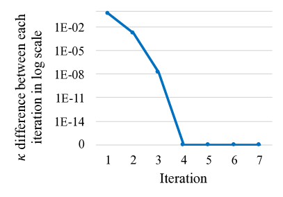
(a) $\kappa$ convergence plot

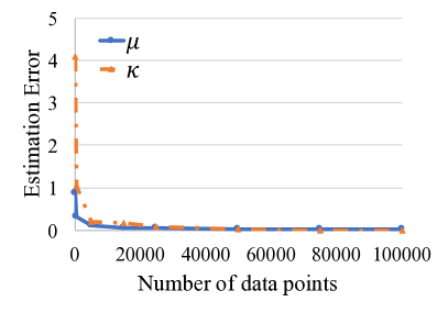
(b) vMF parameter estimation error with $p=100$ and $\kappa=100$

Figure 1: The convergence of the Newton’s method.

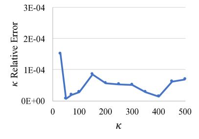
(a) varying $\kappa$ with $p=100$

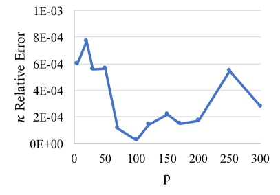
(b) varying $p$ with $\kappa=100$

Figure 2: Estimation error for the concentration parameter $\kappa$

Results on Real-Life Data

Visualization of the Mobility Models

In this set of experiments, we set the number of states to 50 on LA and NY to obtain mobility models. After parameter inference, each state is characterized by: (1) a two-dimensional Gaussian distribution for the spatial location; (2) a one-dimensional Gaussian distribution for the time; and (3) a 30-dimensional vMF distribution for the semantics.

(a) LA dataset state keywords and transitions

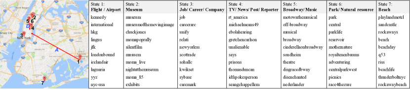
(b) NY dataset state keywords and transitions

Figure 3: The visualization of the mobility models. The digits (1-7) indicate different state locations and the letters (A-D) indicate frequent human movements.

Figure 3 visualizes a number of representative states and some frequent transitions among them. We plot the mean location of some states as well as the top-10 keywords from the vocabulary whose embeddings are the closest to the vMF mean directions. Most of the top-10 keywords for the same state carry consistent and clear semantics. For example, for the Baseball state on the LA dataset: homeruns is a specific baseball term; dodgers is the baseball team in LA; giants is the baseball team in San Francisco; 162 indicates that there are 162 games for each team in the Major League Baseball (MLB) season; and the rest six keywords are all related to baseball too. We have examined the center locations of the states, and found that the geographical locations well match the semantic meanings of different states.

Another interesting finding is that in LA dataset, the mean direction of the General Sports state lies in-between the Basketball state and the Baseball state in the embedding space. Also, the concentration parameter $\kappa$ for General Sports state is lower than Basketball and Baseball state. Such phenomenon intuitively makes sense since General Sports is a broader topic and the semantics of the tweets are more scattered.

We have also observed some interesting state transitions. As shown in Figure 3, the following transitions receive high probabilities in the SHMM model: (A) moving from airports to restaurants; (B) enjoying beach activities at the Venice beach, and then moving around for other leisure activities; (C) going to concerts after having food; (D) watching shows at Broadway and then having other sightseeing activities in NYC Downtown. These high-probability transitions match people’s movements in the real world well.

Performance for Next Location Prediction

Figure 4 shows the performance of next location prediction for different mobility models. It can be seen that our SHMM model outperforms the state-of-the-art GMove model by 3.2% on average. The performance difference shows that the text embedding can better capture the semantics of text messages and reduce text sparsity. Also, the vMF distribution unleashes the discriminative power of text embeddings in a directional metric space.

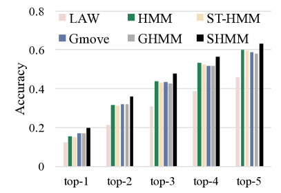
(a) LA

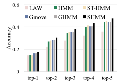
(b) NY

Figure 4: The accuracies of top-$K$ location prediction.

Effects of Parameters

In Figure 5, we study the performance of SHMM and GMove when the number of states varies. We find that the performance of both models generally increases with the number of states. One major reason is that the semantics of people’s activities are separated at finer granularities when the number of states is large. For example, we can see from the LA data set that General Sports, Basketball and Baseball are three separated topics. If the number of states is not large enough, these states may be clustered as one single topic. On the other hand, one caveat for choosing the number of states is that a large number of states could incur high computational overhead, and also harm the interpretability of the result model because the same semantics may be split into duplicate ones.

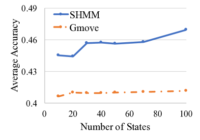
(a) LA

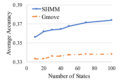
(b) NY

Figure 5: Prediction accuracy v.s. the number of states.

Efficiency Comparison

Finally, we compare the modeling training time between SHMM and GMove when the number of states varies. Generally speaking, the training time of both models increases quadratically with the number of states. The training time of SHMM is obviously smaller than that of GMove, e.g., when the number of states is 100, training SHMM is 25.7% faster on LA and 40.9% faster on NY, and the speedups are even larger when the number of states or the data size increases. This is because SHMM models low-dimensional text embeddings instead of high-dimensional bag-of-words, and thus involves much fewer parameters. In addition, the estimation of the parameters for the vMF distribution is cheap and converges fast.

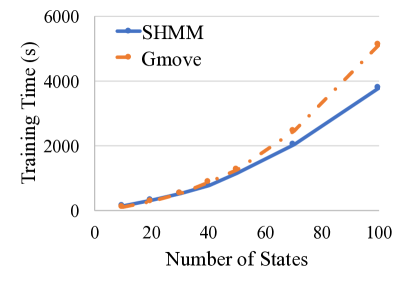
(a) LA

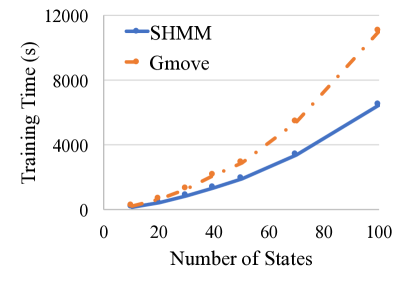
(b) NY

Figure 6: Running time v.s. the number of states.

Related Work

Human mobility modeling. Classic human mobility modeling methods focus on mining the spatiotemporal regularities underlying human movements. Generally, existing mobility modeling methods can be divided into two categories: pattern-based methods and model-based methods. Pattern-based methods aims at discovering specific mobility patterns that occur regularly. Different mobility patterns have been introduced to capture people’s movement regularities, such as frequent sequential patterns (?), periodic patterns (?), and co-location patterns (?). Model-based methods use statistical models to characterize the human mobility, and learn the parameters of the designed model from the observed trace data. Mathew et al. (?) use the hidden Markov model to capture the sequential transition regularities of human mobility; Brockmann et al. (?) proposed that human mobility can be modeled by a continuous-time random-walk model with long-tail distribution; Cho et al. (?) introduce periodic mobility models to discover the periodicity underlying human movements.

While the above mobility modeling methods focus on spatiotemporal regularities without considering text data, recent years are witnessing growing interest in modeling human mobility from semantic trace data (?; ?; ?; ?). Among these works, the state-of-the-art GMove model (?) is the most relevant to our model. Both GMove and SHMM use hidden Markov models to model the generation process of the observed semantic trace data. However, SHMM is different from GMove in that it encodes the semantics of user activities with text embeddings, and uses the vMF distribution to model the text embeddings in the HMM model. As such, the SHMM involves much fewer parameters and well unleashes the discriminative power of text embeddings in a directional metric space.

It is worth mentioning that, there are quite a number of works that uses human trace data for the location prediction problem (?; ?). Typically, they extract features that are important for predicting which place the user tends to visit next based on discriminative models such as recurrent neural networks. While we use location prediction as an evaluation task in our experiments, our work is quite different from these works. Instead of optimizing the performance of location prediction, our focus is to learn interpretable models that reveals the regularities underlying human movements. Besides location prediction, our learned mobility models can be used for many other downstream tasks as well.

vMF-based learning. There are some existing works that utilize vMF distribution for different learning tasks. Dhillon et al. (?) and Banerjee et al. (?) are two pioneering works that use the vMF distributions to handle directional data, which demonstrate inspiring results for text categorization and gene expression analysis. Besides, Gopal and Yang (?) recently applied vMF distributions for clustering analysis, and proposed variational inference procedures for estimating the parameters of the vMF clustering model. Batmanghelich et al. (?) proposed a spherical topic model based on the vMF distribution, which accounts for word semantic regularities in language and has been demonstrated to be superior than multi-variate Gaussian distributions. However, there are no previous works that integrate the vMF distribution with HMMs for semantic trace data. To the best of our knowledge, we are the first to demonstrate that the vMF distribution can work well with HMM for directional data with theoretical guarantees.

Conclusion

We proposed a spherical hidden Markov model for learning interpretable human mobility model from semantic trace data. Our model uses text embeddings to capture the semantics of text messages and integrate the vMF distribution into the hidden Markov model for generating such text embeddings. We have theoretically proved that the Expectation-Maximization algorithm is able to work with vMF distribution, and that the Newton’s method can be applied for efficiently solving the M-step with quadratic convergence rate. Our experiments on synthetic data simulations verify our theoretical analysis. Furthermore, by applying our model to real-life semantic trace datasets, we are able to obtain highly interpretable mobility models, which intuitively make sense and outperform baseline models for downstream tasks like location prediction.

References

- [Abramowitz and Stegun 1964] Abramowitz, M., and Stegun, I. A. 1964. Handbook of mathematical functions: with formulas, graphs, and mathematical tables, volume 55. Courier Corporation.
- [Amos 1974] Amos, D. E. 1974. Computation of modified bessel functions and their ratios. Mathematics of Computation 28(125):239–251.
- [Arora, Liang, and Ma 2016] Arora, S.; Liang, Y.; and Ma, T. 2016. A simple but tough-to-beat baseline for sentence embeddings.
- [Balachandran, Viles, and Kolaczyk 2013] Balachandran, P.; Viles, W.; and Kolaczyk, E. D. 2013. Exponential-type inequalities involving ratios of the modified bessel function of the first kind and their applications. arXiv preprint arXiv:1311.1450.
- [Banerjee et al. 2005] Banerjee, A.; Dhillon, I. S.; Ghosh, J.; and Sra, S. 2005. Clustering on the unit hypersphere using von mises-fisher distributions. Journal of Machine Learning Research 6(Sep):1345–1382.
- [Batmanghelich et al. 2016] Batmanghelich, K.; Saeedi, A.; Narasimhan, K.; and Gershman, S. 2016. Nonparametric spherical topic modeling with word embeddings. arXiv preprint arXiv:1604.00126.
- [Baum et al. 1970] Baum, L. E.; Petrie, T.; Soules, G.; and Weiss, N. 1970. A maximization technique occurring in the statistical analysis of probabilistic functions of markov chains. The annals of mathematical statistics 41(1):164–171.
- [Brockmann, Hufnagel, and Geisel 2006] Brockmann, D.; Hufnagel, L.; and Geisel, T. 2006. The scaling laws of human travel. arXiv preprint cond-mat/0605511.
- [Chen et al. 2015] Chen, Y.-H.; Wei, D.; Newstadt, G.; DeGraef, M.; Simmons, J.; and Hero, A. 2015. Parameter estimation in spherical symmetry groups. IEEE Signal Processing Letters 22(8):1152–1155.
- [Cheng et al. 2011] Cheng, Z.; Caverlee, J.; Lee, K.; and Sui, D. Z. 2011. Exploring millions of footprints in location sharing services. In ICWSM.
- [Cho, Myers, and Leskovec 2011] Cho, E.; Myers, S. A.; and Leskovec, J. 2011. Friendship and mobility: User movement in location-based social networks. In KDD, 1082–1090.
- [Dempster, Laird, and Rubin 1977] Dempster, A. P.; Laird, N. M.; and Rubin, D. B. 1977. Maximum likelihood from incomplete data via the em algorithm. Journal of the royal statistical society. Series B (methodological) 1–38.
- [Dhillon and Sra 2003] Dhillon, I. S., and Sra, S. 2003. Modeling data using directional distributions. Technical report, Technical Report TR-03-06, Department of Computer Sciences, The University of Texas at Austin.
- [Fisher 1953] Fisher, R. 1953. Dispersion on a sphere. In Proceedings of the Royal Society of London A: Mathematical, Physical and Engineering Sciences, volume 217, 295–305. The Royal Society.
- [Giannotti et al. 2007] Giannotti, F.; Nanni, M.; Pinelli, F.; and Pedreschi, D. 2007. Trajectory pattern mining. In KDD, 330–339.
- [Gonzalez, Hidalgo, and Barabasi 2008] Gonzalez, M. C.; Hidalgo, C. A.; and Barabasi, A.-L. 2008. Understanding individual human mobility patterns. arXiv preprint arXiv:0806.1256.
- [Gopal and Yang 2014] Gopal, S., and Yang, Y. 2014. Von mises-fisher clustering models. In ICML, 154–162.
- [Kalnis, Mamoulis, and Bakiras 2005] Kalnis, P.; Mamoulis, N.; and Bakiras, S. 2005. On discovering moving clusters in spatio-temporal data. In SSTD, 364–381.
- [Kitamura et al. 2000] Kitamura, R.; Chen, C.; Pendyala, R. M.; and Narayanan, R. 2000. Micro-simulation of daily activity-travel patterns for travel demand forecasting. Transportation 27(1):25–51.
- [Le and Mikolov 2014] Le, Q., and Mikolov, T. 2014. Distributed representations of sentences and documents. In ICML, 1188–1196.
- [Li et al. 2010] Li, Z.; Ding, B.; Han, J.; Kays, R.; and Nye, P. 2010. Mining periodic behaviors for moving objects. In KDD, 1099–1108.
- [Liu and et al. 2016] Liu, Q., and et al. 2016. Predicting the next location: A recurrent model with spatial and temporal contexts. In AAAI, 194–200.
- [Mathew, Raposo, and Martins 2012] Mathew, W.; Raposo, R.; and Martins, B. 2012. Predicting future locations with hidden markov models. In UbiComp, 911–918.
- [Mikolov et al. 2013a] Mikolov, T.; Chen, K.; Corrado, G.; and Dean, J. 2013a. Efficient estimation of word representations in vector space. arXiv preprint arXiv:1301.3781.
- [Mikolov et al. 2013b] Mikolov, T.; Sutskever, I.; Chen, K.; Corrado, G. S.; and Dean, J. 2013b. Distributed representations of words and phrases and their compositionality. In NIPS, 3111–3119.
- [Segura 2011] Segura, J. 2011. Bounds for ratios of modified bessel functions and associated turán-type inequalities. Journal of Mathematical Analysis and Applications 374(2):516–528.
- [Simpson and Spector 1984] Simpson, H. C., and Spector, S. J. 1984. Some monotonicity results for ratios of modified bessel functions. Quarterly of Applied Mathematics 42(1):95–98.
- [Wang et al. 2015] Wang, Y.; Yuan, N. J.; Lian, D.; Xu, L.; Xie, X.; Chen, E.; and Rui, Y. 2015. Regularity and conformity: Location prediction using heterogeneous mobility data. In KDD, 1275–1284.
- [Wu et al. 2015] Wu, F.; Li, Z.; Lee, W.-C.; Wang, H.; and Huang, Z. 2015. Semantic annotation of mobility data using social media. In WWW, 1253–1263.
- [Ying et al. 2011] Ying, J. J.; Lee, W.; Weng, T.; and Tseng, V. S. 2011. Semantic trajectory mining for location prediction. In GIS, 34–43.
- [Zhang et al. 2014] Zhang, C.; Han, J.; Shou, L.; Lu, J.; and Porta, T. F. L. 2014. Splitter: Mining fine-grained sequential patterns in semantic trajectories. PVLDB 7(9):769–780.
- [Zhang et al. 2016a] Zhang, C.; Zhang, K.; Yuan, Q.; Zheng, L.; Hanratty, T.; and Han, J. 2016a. Gmove: Group-level mobility modeling using geo-tagged social media. In KDD, 1305–1314.
- [Zhang et al. 2016b] Zhang, C.; Zhou, G.; Yuan, Q.; Zhuang, H.; Zheng, Y.; Kaplan, L. M.; Wang, S.; and Han, J. 2016b. Geoburst: Real-time local event detection in geo-tagged tweet streams. In SIGIR, 513–522.
- [Zhang et al. 2017] Zhang, C.; Zhang, K.; Yuan, Q.; Peng, H.; Zheng, Y.; Hanratty, T.; Wang, S.; and Han, J. 2017. Regions, periods, activities: Uncovering urban dynamics via cross-modal representation learning. In WWW, 361–370.