Worm quantum Monte-Carlo study of phase diagram of extended Jaynes-Cummings-Hubbard model

Abstract

Herein, we study the extended Jaynes-Cummings-Hubbard model mainly by the large-scale worm quantum Monte-Carlo method to check whether or not a light supersolid phase exists in various geometries, such as the one-dimensional chain, square lattices or triangular lattices. To achieve our purpose, the ground state phase diagrams are investigated. For the one-dimensional chain and square lattices, a first-order transition occurs between the superfluid phase and the solid phase and therefore there is no stable supersolid phase existing in these geometries. Interestingly, soliton/beats of the local densities arise if the chemical potential is adjusted in the finite-size chain. However, this soliton-superfluid coexistence can not be considered as a supersolid in the thermodynamic limit. Searching for a light supersolid, we also studied the Jaynes-Cummings-Hubbard model on triangular lattices, and the phase diagrams are obtained. Through measurement of the structural factor, momentum distribution and superfluid stiffness for various system sizes, a supersolid phase exists stably in the triangular lattices geometry and the regime of the supersolid phase is smaller than that of the mean field results. The light supersolid in the Jaynes-Cummings-Hubbard model is attractive because it has superreliance, which is absent in the pure Bose-Hubbard model. We believe the results in this paper could help search for new novel phases in cold-atom experiments.

I introduction

A supersolid $(SS)$ phase is a novel quantum state with is both superfluid and solidcondensation ; sov ; speculations ; BEC3 . In the past ten years, with the great progress of quantum manipulation of atomic technology, scientists have tried to observe the $SS$ phase in ultra-cold atomic systems. A breakthrough occurred in 2017 when two groups observed the $SS$ phase in cold atomssupersolid formation ; supersolid properties . In 2019, three independent groups found the $SS$ phase experimentallydipolar quantum gas ; DipolarQuantum Droplets ; supersolid behaviors .

Physical models include the extended Bose-Hubbard (BH) modelSupersolids versus Phase Separation , the two-component BH model2CM1 ; 2CM2 ; 2CM3 , the paired BH modelliangP1 ; guoP2 ; wangP3 ; chenP4 ; troyP5 ; guoP6 , the Bose-Fermi mixture systemBF1 ; BF2 , the Fermion systemfm1 and the spin system2spin1 ; spin2 , the $SS$ phase in spin-orbit coupled systemsUltracold Atomic Bose Condensates , the BH model with next-nearest neighborhood interactions next , and dipolar bosons5 .

The $SS$ model mentioned earlier does not involve the quantum optical cavity model and its extensions. Most quantum optics models based on single-cavity systems have interesting phases, such as the super-radiation solid phase in a single-cavity system coupled with an optical lattice A Superradiant Solid , that is, coexistence of a super-radiation order and an atomic solid order. However, here we will extend the single-cavity case to the lattices of multiple cavities with various geometries, i.e. one-dimensional lattices, square lattices, and triangular lattices. The Jaynes-Cummings models sitting in each lattice site form the so-called Jaynes-Cummings-Hubbard (JCH)QED ; SMI model with additional photons hopping between cavities.

Experimentally, the JCH model can be realized by a coupled-transmission-line resonatorLow or trapped ionsExp . Moreover, theoretical studiesMF ; MF1 ; GL ; strong and reliable numerical methods, such as the density matrix renormalization group algorithm(DMRG)AM ; Fermionized and the quantum Monte-Carlo(QMC)Dynamical critical ; zhaojize method are also investigated. Furthermore, various topics including fractional quantum Hall PhysicsFractional , quantum transportQuantum transport , quantum-state transmissionQuantum-state , on-site disorderMF1 ; Disorder and phase transitionsMF ; MF1 are explored intensively.

In regards to the anti-ferromagnetic correlation between the excitations of each atom, the JCH model can be considered as an extended JCH model. There are still interesting questions to be discussed for the extended JCH models.

1. For pure hard-core BH models, there is no $SS$ phase in the bipartite lattices. It is still not clear whether or not there is a $SS$ phase in the JCH model at the bipartite lattices, as is the case for JCH models on one-dimensional lattices and square lattices. Meanwhile, Ref. light-ss shows the $SS$ phase with nearest interactions between cavities by using the cluster mean field method. They also expect a reliable method to vindicate their findings.

2. In previous work guolijuan , we used the DMRG methodDMRG1 ; DMRG2 to give the paired $SS$ phase for the JCH model on different ladders. Furthermore, for the JCH system on the two-dimensional triangular lattice, we presented the mean field (MF) result to give a preliminary phase diagram using the cluster mean field method. Although the cluster size has up to 36 sites, we still need more reliable methods to confirm the stability of the $SS$ phase.

To clarify the above questions, we mainly use the large-scale worm algorithm of the quantum Monte-Carlo (wQMC) methodwqmc1 ; wqmc2 ; wqmc3 ; wqmc4 , to simulate the model on various geometries.The global phase diagram by the MF method is plotted as background.

We find that, for bipartite lattices, there is no light $SS$ phase in the extended JCH model. The previously predicted $SS$ phase by the MF methodlight-ss is not stable, i.e., the transition between the solid phase to the superfluid phase is of first order with obvious jumping of the order parameters such as the superfluid stiffness and structural factors. To search for the light $SS$ phase, the JCH model on the two-dimensional triangular lattices is studied and a stable light $SS$ phase is found.

The outline of this paper is as follows: Sec. II introduces the model, methods and the measured quantities. Sec. III shows the results on bipartite lattices such as 1D and 2D square lattices. Sec. IV gives the results of the JCH models on triangular lattices. Conclusions are made at the end in Sec. V.

II model, methods and the measured quantities

II.1 Model and its mapping

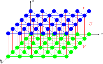
Figure 1: (Color online) The mapped two-layer triangular lattices for the JCH model, where the top and bottom layers are denoted as photon and atom layers respectively. The hopping of the photons $t$, atom-photon coupling $U$, and interactions between atom excitations $V$ are labeled. A one-dimensional chain and a square lattice are illustrated in appendix A.

The extended JCH model includes a nearest repulsion between excitations of the cavities with strength $V$, which is different from the atom-atom repulsion interaction. The model has many cavities and each cavity can be considered a site in the lattices. In each cavity, there is a two-level atom. Simultaneously, photon tunneling between cavities is considered.

To simulate the model conveniently, the model could be mapped unto a pure BH model on two layered geometries, e.g two-layer triangular lattices as shown in Fig.1, where the top layer and bottom layer describe the state of the photon and the level of the atom, respectively. For a specific site r=($x$, $y$), if the two-level atom sits in the ground state, then the state at ($x$, $y$, $z=1$) should be empty and the excited state, occupied. Similarly, the state at ($x$, $y$, $z=2$) describes the photon number in each cavity.

In comparison to the pure BH model, the interaction and hopping between layers are different. In the photon layer, only photon hopping without repulsion exists and in the atom layer, only repulsion without the hopping term exists. The extended JCH Hamiltonian is defined as

$$H= \sum_{i}(H_{i}^{JC}-\mu n_{i})-t\sum_{\langle i,j\rangle}(a_{i}^{\dagger}a_{j}+\rm H.c.)$$ (1)

$$+\sum_{\langle i,j\rangle}Vn_{i}^{\sigma}n_{j}^{\sigma},$$

where the total number of excitations is $\rho\equiv\sum_{i}{n}_{i}=\sum_{i}(n_{i}^{\sigma}+n_{i}^{a})$, $\mu$ is the chemical potential, $a_{i}^{\dagger}$ and $a_{i}$ are respectively the photon creation and annihilation operators at lattice site $i$, and the term $(a_{i}^{\dagger}a_{j})$ with strength $t$ represents the photon hopping between cavities. The on-site coupling between the photons and the atom on each site $i$ can be described by the JC Hamiltonian $H_{i}^{JC}$

$$H_{i}^{JC}= \omega n_{i}^{a}+\varepsilon n_{i}^{\sigma}+U(a_{i}^{\dagger}\sigma_{i}+a_{i}\sigma_{i}^{\dagger}),$$ (2)

where $U$ is the atom-photon coupling strength and represents the tunneling between layers, $\omega$ is the frequency of the model of the photon creation and annihilation operators at lattice site $i$, and, $\varepsilon$ is the transition frequency between two energy levels. For simplicity, we restrict $\omega=\varepsilon=0$. Operators $n_{i}^{a}=a_{i}^{\dagger}a_{i}$ and $n_{i}^{\sigma}=\sigma_{i}^{\dagger}\sigma_{i}$ are the photon number and the number of excitations of the atomic levels, respectively. The Pauli matrices $\sigma_{i}^{\dagger}$ ($\sigma_{i}$) represent the raising (lowering) operators for the atom levels.

II.2 Methods and the quantities measured

The conclusive results are mainly obtained by the wQMC method, and the details can be seen in Refs. wqmc1 ; wqmc2 ; wqmc3 ; wqmc4 . Here, in the real simulations, the inverse temperature $\beta=1/k_{b}T$ takes larger values, namely, $\beta=100,~{}500,~{}\cdots,~{}1500$ for allowing the systems to converge to the ground state. We have tried a stochastic series expansion QMC methodexpansion ; directed loops . However, due to local atom-photon coupling and the no-hopping term between each atom layer, the updating efficiency is very slow in low temperature regimes. The needed quantities for the worm QMC algorithm are:

1. Local photon density $\rho_{i}^{a}=\left\langle n_{i}^{a}\right\rangle$ and local atom excitation $\rho_{i}^{\sigma}=\left\langle n_{i}^{\sigma}\right\rangle$.
   

2. Superfluid stiffnessstiff

   $$\rho_{s}=\sum_{r=1}^{d}\frac{L^{2-d}\left\langle W_{r}\right\rangle^{2}}{2d\beta t},$$ (3)

   where $W_{r}$ is the winding number of the photons in the upper layer in the $x$ or $y$ direction. The stiffness characterizes the non-diagonal long range order of the system.

3. Structural factor of photons, given by

   $$S(\mathbf{Q})/N=\left\langle\rho_{\mathbf{Q}}\rho_{\mathbf{Q}}^{\dagger}\right\rangle$$ (4)

   where $\rho_{\mathbf{Q}}=(1/N)\sum_{i}n_{i}^{a}\exp(i\mathbf{Q}\mathbf{r}_{i})$, $N=L\times L$ is the total number of physical sites for 2D systems and $N=L$ for 1D systems. For a one-dimensional lattice, the wave vector is at $\mathbf{Q}=(\pi,0)$. In real space, the density of excitation obeys configurations of the form ($101010\cdots$) or ($010101\cdots$). The phase here is called the solid I $(SI)$ phase. For square lattices, the solid with $\mathbf{Q}=(\pi,\pi)$ is also called the $SI$ phase.

   For the two-dimensional triangular lattices, the wave vector is at $\mathbf{Q}=(4\pi/3,0)$ and excitation densities obey configurations of the form ($001001\cdots$) or ($110110\cdots$). The densities are $1/3$ and $2/3$, and called the $SII$ phase and $SIII$ phase, respectively.

4. Momentum distribution given by

   $$n\left(\textbf{k}\right)=\frac{1}{N}\sum\limits_{j,j^{{}^{\prime}}}\left\langle a_{j}^{\dagger}a_{j^{{}^{\prime}}}\right\rangle e^{i\textbf{k}\left(\textbf{r}_{j}-\textbf{r}_{j^{{}^{\prime}}}\right)}$$ (5)

   In the $SS$ phase, $S(\mathbf{Q})/N$ and $\rho_{s}^{x(y)}$ are both nonzero in the thermodynamic limit. Moreover, the global phase diagram is plotted with $\Psi=\langle a\rangle$ in the MF frame, which is illustrated in appendix C for completeness.

   The above quantities of $\rho$, $S(\pi)/L$ and energy density $E$ are calculated by exact diagonalization and wQMC methods.The results are consistent with each other and shown in appendix B.

III Results for the JCH model on bipartite lattices

In this section, we focus on the results of the JCH models on both the 1D and square lattices.

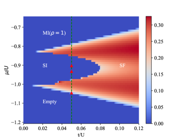
Figure 2: (Color online) Phase diagram and the detailed description of $\Psi$ for the 1D hardcore extended JCH model with $V/U=0.4$ by the MF method. The green dashed line labels the position scanning by wQMC and the red triangular symbols are the phase boundaries given by the wQMC method.

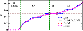
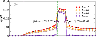
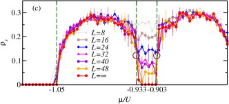
Figure 3: (Color online) Monte Carlo results of (a) excitation densities $\rho$ (up to $L=96$), (b) structural factors $S(\pi)/L$ and (c) superfluid stiffness $\rho_{s}$ as a function of $\mu/U$ with system sizes $L=8,~{}16,~{}24,~{}32,~{}40,~{}48$ and $\infty$ at parameters $V/U=0.4$ and $t/U=0.05$.

III.1 Hardcore 1D JCH model

For the 1D hardcore extended JCH model, the maximum number of photons is restricted to be one in each cavity. It is well known that the number of photons is not fixed in a grand canonical ensembleDynamical critical . Therefore, the softcore photon system has to be checked and the Physics does not changeguolijuan .

Fig. 2 shows the MF phase diagramopt ; cluster2 ; cluster3 ; cluster4 ; cluster5 , which contains the empty, $SI$, $SS$, $SF$ and $MI$($\rho=1$) phases, by plotting $\Psi$ in the plane ($t/U$, $\mu/U$).

As $t/U$ is small, and $\mu/U\textless-1$, the system is in an empty phase with $\rho=0$ and $\Psi=0$. The system sits in the $MI$($\rho=1$) phase if $\mu/U>-0.83$. Moreover, the $SI$ phase appears between the two regimes. As $t/U$ gets larger, the system enters the $SF$ phase. As discussed in Ref. SMI , for a large hopping $t/U$, the ground state energy becomes negative and can be made arbitrarily small by increasing the total number of excitations. Here, since the maximum number of photons is fixed, the $SF$ remains stable.

The question about whether or not the $SS$ phase could exist in the thermodynamic limit can now be verified by the wQMC method. Fig. 3(a) shows the results of excitation densities as a function of $\mu/U$ with system sizes $L=8,~{}16,~{}24,~{}32,~{}40,~{}48,~{}64,~{}96$ and $\infty$. If $\mu/U$ increases, the excitation density increases. When $\mu/U$ increases to about $-0.9$, a plateau of density ($\rho=0.5$) appears.

Fig. 3(b) shows the structural factor $S(\pi)/L$ of photons obtained as a function of $\mu/U$ with sizes $L=32,~{}40,~{}48$ and $\infty$ with the sufficiently low temperature $\beta=1500$.

Consistent with the excitation density, nonzero $S(\pi)/L$ has a platform in the interval $-0.933\textless\mu/U\textless-0.903$, and simultaneously, superfluid stiffness $\rho_{s}^{x}$ becomes zero in the thermodynamic limit in Fig. 3(c). The two signatures clearly demonstrate that a $SI$ phase exists in the regimes.

By doping vacancies or excitations on the $SI$ phase, $S(\pi)/L$ converges to zero and $\rho_{s}^{x}$ becomes non-zero at $L\rightarrow\infty$. The behavior of the jump at those two ends of the platform represents clear first-order transitions between the $SF$ and $SI$ phases, and obviously no $SS$ phase exists. The $SS$ phase is unstable against the phase separationseparation ; separation2 ; separation3 ; BF3 .

Here, we just show the quantities sampled from the upper layer. Moreover, the phase transition points from the empty phase to the $SF$ phase, the predictions by the MF and wQMC methods being completely the same at $\mu/U=-1.05$.

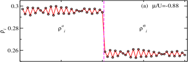
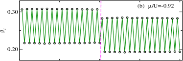
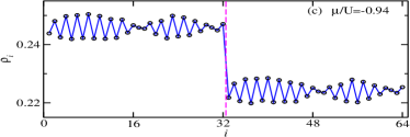
Figure 4: (Color online) Local photon density $\rho^{a}_{i}$, local atom excitation density $\rho^{\sigma}_{i}$ and solitonic signature in upper and bottom layers as a function of position $i$ with $V/U$=0.4 and $t/U=0.05$. (a)$\mu/U$=-0.88, with on-site excitation density $\rho>1/2$. (b) $\mu/U$=-0.92, with $\rho=1/2$. (c) $\mu/U$=-0.94, with $\rho<1/2$.

In the regime $-1.05\textless\mu/U\textless-0.933$, $S(\pi)/L$ for a finite system size is not zero (see Fig. 3(b)). To further understand $S(\pi)/L$ , we illustrate the local photon densities $\rho^{a}_{i}$ and the local atom excitation density $\rho^{\sigma}_{i}$ function of position $i$ under different values of chemical potential $\mu$ in Fig. 4. The commensurate density distribution arises in Fig. 4(b), which confirms the periodic ground state long-range crystalline order in the solid phase. The on-site excitation density in the solid phase is calculated to be $\rho=1/2$, which includes both photons and atoms. Therefore e.g. the local photon density $\rho^{a}_{i}$ in the upper layer oscillates between $0.19$ and $0.31$ with the average value being $0.25$.

In Figs. 4(a) and (c), the beats or soliton patterns6 ; beats arise, which means changing the chemical potential $\mu$ (or removal/addition of the photons) will give rise to the soliton patterns. Only the uniform density oscillation is seen but no beats or soliton patterns appear in Fig. 4(b). The number of solitons will increase as the photons are further added or removed, meanwhile the density oscillation becomes weak. In other words, starting with the $SI$ phase, and changing the chemical potential $\mu$ leads to a solitons+$SF$ crossover instead of the $SS$ phase. In the thermodynamic limit, the crossover region will vanish, and the system will experience first-order transitions immediately.

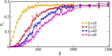
Figure 5: (Color online) Simulation results by the wQMC method of superfluid stiffness $\rho_{s}$ as a function of $\beta$ for the hardcore 1D JCH model. The parameters are $V/U=0.4$, $\mu/U=-1$, and $t/U=0.05$, and the system sizes are $L=16,~{}32,~{}40$ and $48$, respectively.

Usually, for the BH model, the ground state will be reached if $\beta t>L$. For the JCH model, through careful checking, $\beta$ should be much larger than $L/t$. In particular, for $L=48$, $\rho_{s}$ should reach convergence here at $\beta=48/0.05\approx 1000$. However, as shown only in Fig. 5 with $L=16,~{}32,~{}40$ and $48$, the temperature should be sufficiently low enough for a ground state. Therefore, in the section, $\beta$ is chosen as 1500.

III.2 Hard core JCH model on square lattice

Although the square lattice is a bipartite lattice, the Physics between the 1D and 2D models may be different. We still need to perform powerful wQMC simulations on the 2D geometries. Various global phase diagrams in the MF frame have been shown in Ref. light-ss . The purpose here is to check the results by the reliable wQMC method. As shown in Fig. 6, we also set $t$ at the fixed value $t/U=0.025$ and then measured $\rho$, $S(Q)/N$, and $\rho_{s}$ as a function of $\mu/U$ for the JCH model on the square lattices. The inverse temperature is $\beta=1000$ and system sizes are $L=4,~{}8,~{}12$ and $16$, respectively.

In a manner similar to the 1D model, we still see the $SI$ phase (0,1,0,1) order in both directions and the wave vector is Q=($\pi$, $\pi$) in the range of $-1.960\textless\mu/U\textless-1.698$, with signatures $\rho=0.5$, $S(Q)/N\neq 0$, and $\rho_{s}=0$. At the two ends of the $SI$ phase, $S(Q)/N$ and $\rho_{s}$ change discontinuously, which clearly indicates that no $SS$ phase exists in the square lattices. The histogram of $S_{T}(Q)/N$ obtained at the phase transition point in Fig. 6(d) demonstrates the two peaks which also indicate the first-order transition between the $SI$ and $SF$ phases. Here, the total structure factor $S_{T}(Q)/N$ is defined by replacing $n_{i}^{a}$ with $n_{i}^{\sigma}+n_{i}^{a}$, as a signature of the double peaks is more clear. In addition, we observe empty, $SF$ and $MI$($\rho=1$) phases as expected. The critical points of the empty-$SF$ phase transition is -2.06, and similarly for the results from the MF methods.

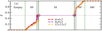
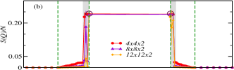
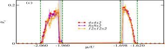
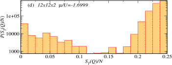
Figure 6: (Color online) Simulation results by the wQMC method of (a) $\rho$ and (b) $S(Q)/N$ (c) $\rho_{s}$ as a function of $\mu/U$ for the JCH model on the square lattices. The parameters are $t/U=0.025$, $\beta=1000$ with $L=4,~{}8,~{}12$, respectively. Dashed regimes are for first-order transitions. (d) Histogram of $S_{T}(Q)/N$ obtained at the phase transition point $\mu/U=-1.6999$ for the system size $L=12$.

IV Results for the JCH models on triangular lattices

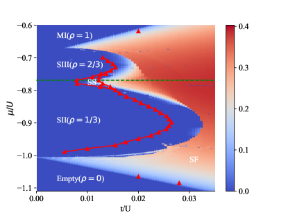
Figure 7: The triangular lattices phase diagram and the detailed description of $\Psi$ for 2D JCH model with $V/U=0.4$ by the MF method. The red triangular symbols are the phase boundaries given by the wQMC method, and the green dashed line labels the cut scanning with $\mu/U=-0.77$.

The BH model on the triangular lattices has been studied extensivelytri2 ; tri3 ; zhangP7 ; Mishra15 ; zhangT1 ; zhangT2 ; zhangT3 , Fig. 7 shows the phase diagram obtained from the MF method, which contains the empty, $SII$, $SIII$, $MI$($\rho=1$), $SS$ and $SF$ phases in the plane ($t/U$, $\mu/U$). The colored symbols denote the numerical results obtained by wQMC methods. The phase diagram of the pure BH model on the triangular lattices has been obtainedtri2 ; tri3 , and is symmetric about the particle-hole symmetric point $\mu/V=3$. Here, for the JCH model, the phase diagram is not symmetric due to the atom-photon coupling, and a similar “symmetric point” can be found between the $SII$ and $SIII$ phases, which locates itself at about $\mu/U=-0.775$ (green dashed line) through the wQMC method.

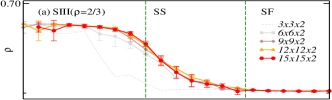
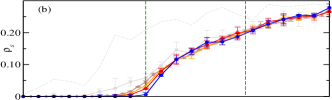
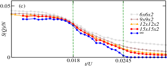
Figure 8: Simulation results by the wQMC method of (a) $\rho$, (b) $S(Q)/N$, and (c) $\rho_{s}$ as a function of $t/U$ for the JCH model on the triangular lattices. The parameters are $\mu/U=-0.77$, $\beta=500$ and the system sizes are $L\times L\times 2$, where $L=6,~{}9,~{}12$ and $15$, respectively.

The system is in an empty phase when $\mu/U$ is very small (bottom of the phase diagram) and in the $MI$($\rho=1$) phase when $\mu/U$ is large (top of the phase diagram). In the middle regimes, around $\mu/U=-0.775$, the $SII$ ($\rho=1/3$) and $SIII$ ($\rho=2/3$) phases emerge. As $t/U$ gradually increases, the system enters into the $SF$ phase. In a manner similar to the pure BH model, the phase transitions between them are as follows: the solid-$SF$ transition is first order, and the $SF$-$MI$ transitions are continuous.

Surrounded by the two types of solid phases and the $SF$ phase, the $SS$ phase emerges in the closed regime illustrated by lines with triangular symbols as shown in Fig. 7.

Fig. 8 shows the wQMC simulations of $\rho$, $\rho_{s}$, $S(Q)/N$ as a function of $t/U$. The parameters are $\mu/U=-0.77$, inverse temperature $\beta=500$ and the mapped system sizes are $L\times L\times 2$ , where $L=3,~{}6,~{}9,~{}12,~{}15$ and $\infty$, respectively. In the regimes of $t/U\textless 0.018$, the systems are trapped in the $SIII$ ($\rho=2/3$) solid phase, with signature of $S(Q)/N\neq 0$ and $\rho_{s}=0$. When $t/U$ increases, induced vacancies lead to the decrease from the excitation density and both $S(Q)/N$ and $\rho_{s}$ are nonzero. In particular, in the region of $0.018\leq t/U\leq 0.0245$, the system sits in the $SS$ phase stably in some special parameter regime of the triangular JCH model.

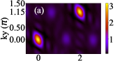
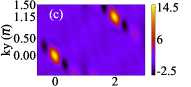
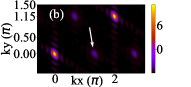
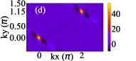
Figure 9: Distribution of $Sq\left(kx,ky\right)$ and momentum distribution $n\left(kx,ky\right)$ for the $SS$ phase on the triangular lattices with $L\times L\times 2$. (a) $Sq\left(kx,ky\right)$, $L$= 6 (b) $Sq\left(kx,ky\right)$, $L$= 12 (c) $n\left(kx,ky\right)$, $L$= 6 (d) $n\left(kx,ky\right)$, $L$= 12. The parameters are $\mu/U=-0.77$, $\beta=500$, $t/U=0.015$.

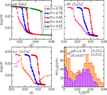
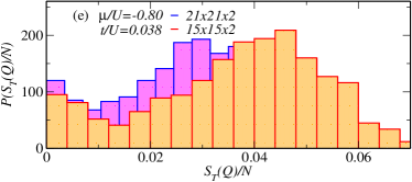
Figure 10: Simulation results by the wQMC method of $S(Q)/N$ as a function of $t/U$ for the JCH model on the triangular lattices with parameter $\beta=500$, the fixed sizes are (a) $L=9$, (b) $L=12$ and (c) $L=15$. The colored lines denote different values of $\mu/U$ near the phase. (d) Histogram of $S_{T}(Q)/N$ obtained at the phase transition point $\mu/U=-0.78$ and $t/U=0.017$ for the system size of $L=15$ (yellow color) and $21$ (purple color). (e) Histogram of $S_{T}(Q)/N$ obtained at the phase transition point $\mu/U=-0.80$ and $t/U=0.038$ for the system size of $L=15$ (yellow color) and $21$ (purple color).

Examples for the structure factor are shown in Figs. 9(a)-(b), with $L=6$ and $12$ respectively. The two peaks of $S\left(Q\right)$ with maximum value are located at $(0,0)$ and ($2\pi$, $1.15\pi$) because of a partially translational invariance between densities on lattices. In the $SS$ phase at $\mu/U=-0.77$, $t/U=0.015$, we observe a second maximum which is at $Q=(4/3\pi,0)$, with a $\sqrt{3}\times\sqrt{3}$ diagonal long-range order of filling 2/3Jap ; sqrt3 . This peak indicates the presence of a density ordering in the liquid phase, which defines a $SS$. The momentum distribution in Eq. (5) is also obtained, which was observed experimentally. The two peaks of $n\left(k\right)$ with maximum value are located at $(0,0)$ and ($2\pi$, $1.15\pi$), which is the sign of the $SF$ phase, as shown in Figs. 9(c)-(d).

In the hard-core BH model on the triangular lattices, it has been verified that the types of $SS$-$SF$ transitions are first-order or continuous, depending on the regimes of chosen $\mu$ Jap ; sqrt3 . In Fig. 8, with the fixed parameter $\mu/U=-0.77$, we show the curves of $\rho$, $\rho_{s}$, and $S(Q)/N$ as a function of $t/U$ for the JCH model, and the $SS$-$SF$ phase transition is continuous, and the $SII$-$SS$ phase transition is also continuous.

In Fig. 10, we carefully examine the phase transitions among the $SII$, $SIII$, $SS$ and $SF$ phases, with respect to the deviation from the parameter of $\mu/U=-0.77$. Figs. 10(a), (b) and (c) show the $S(Q)/N$ as a function of $t/U$ with system sizes $L$=$9,12$ and $15$, respectively. When $\mu/U=-0.78$, the first-order phase transition occurs between the $SII$ and the $SS$ phase.

Simultaneously, the transition from the $SS$ to the $SF$ phases is continuous. It is still continuous when $\mu/U=-0.79$. When $\mu/U=-0.80$, it is found that there is an obvious jump of the $S(Q)/N$ at $t/U=0.031$ (see the red line in Fig. 8(c)). The bimodal distribution of total structural factors $S_{T}(Q)/N$ in Fig. 10(d) and Fig. 10(e) are displayed to confirm the first order (discontinuous) property of the $SS$-$SF$ phase transition.

V conclusion

In conclusion, we have systematically investigated the hard-core JCH model on one-dimensional lattices, square lattices and triangular lattices using the wQMC method. Three important quantities, the excitation densities $\rho$, structural factors $S(Q)/N$, and superfluid stiffness $\rho_{s}$ are measured.

For the bipartite lattice such as the one-dimensional chain and square lattices, we clarified that the previously found $SS$ phase by the MF method is not really stable. By doping vacancies or excitations on the $SI$ phase, $S(Q)/N$ and $\rho_{s}^{x}$ jump obviously in the thermodynamic limit and a two-peak histogram of $S_{T}(Q)/N$ emerges, which represents clear first-order transitions between the $SF$ and $SI$ phases. We found that the phase boundaries between the empty-$SF$ phase transition and the $MI$-$SF$ phase transition are the same with $MF$ methods.

For the JCH model on the triangular lattices, the phase diagram obtained from the MF method is shown as background, which contains the empty, $SII$, $SIII$, $MI$, $SS$ and $SF$ phases in the $t$-$\mu$ plane. The numerical results obtained by the wQMC methods are also included to locate the regimes of the stable $SS$ phase in the thermodynamic limit. The peaks of $Sq(kx,ky)$ and the experimentally observed momentum distribution $n(kx,ky)$ confirm the presence of the $SS$ phase.

Surrounded by three different phases, the phase transitions between the $SS$ phase and other phases are more complicated and interesting. The $SIII$-$SS$ transition is confirmed to be continuous. However, the $SII$-$SS$ transition can be obviously first-order, depending on the regimes of $\mu$ chosen. The $SS$-$SF$ transition is similar to that in the hard-core BH model and this transition is first order (far away from the symmetric point) or continuous (near the symmetric point).

Appendix A The geometries of one-dimensional chain and square lattices

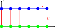
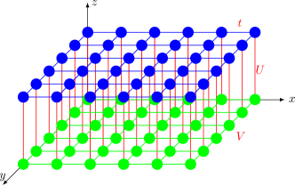
Figure 11: The mapped two-layer one-dimensional chain and square lattices from the JCH model, where the top and bottom layers can be denoted as photon and atom layers respectively. The hopping of photons $t$, atom-photon coupling $U$, and interactions between atoms excitations $V$ are labeled.

In Fig.11 we mapped JCH model a two-layer triangular lattice, here, we show the JCH model geometry of one dimensional chain and square lattices

Appendix B Comparison with exact diagonalization

Before the large-scale simulations, we compare the results of small systems such as $L=4$ by the wQMC method with exact diagonalization at parameters $t/U=0.05$ and $V/U=0.4$. We perform QMC at the fixed temperature $\beta=200$ while exact diagonalization with $\beta=100,~{}200,~{}300,~{}400$ and $500$. The quantities such as the excitation densities $\rho$, the structural factors $S(\pi)/L$, and the energy densities $E$ are shown and consistent with each other.

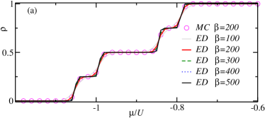
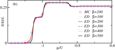
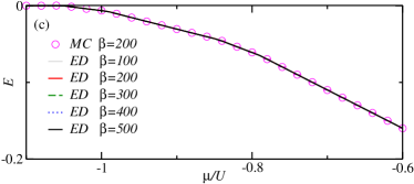
Figure 12: Comparison of the simulation results of the one-dimensional JCH lattice with $L=4$ by both ED and wQMC methods (a) $\rho$ (b) $Sq(\pi)/L$ (c) $E$ for various temperatures $\beta=100-500$.

Appendix C MF methods

In the CMF frame, the total Hamiltonian is taken to be $H_{tot}=H_{mf}+H_{ed}$, where the exactly treated $H_{ed}$ is the Hamiltonian inside the cluster, such as the triangular lattice (ABC) illustrated by a yellow color in Fig. 13.

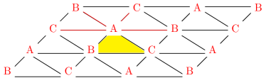
Figure 13: (Color online) A triangular lattice by three sublattices $A$, $B$ and $C$. The triangle denoted by the yellow color is the cluster treated exactly. The interaction and hopping illustrated by the red lines such as AB, AC are decoupled approximately.

The Hamiltonian $H_{mf}$ is given by

$$H_{mf}= -qt\sum_{i,j\in ce}[(a_{i}^{\dagger}+a_{i})\Psi_{j}+(a_{j}^{\dagger}+a_{j})\Psi_{i}-2\Psi_{i}\Psi_{j}]$$ (6)

$$+qV\sum_{i,j\in ce}({n_{i}^{\sigma}\rho_{j}^{\sigma}+n_{j}^{\sigma}\rho_{i}^{\sigma}-\rho_{i}^{\sigma}\rho_{j}^{\sigma}}).$$

Here, the site $A$ connects $B$ and $C$ by the four red lines. Therefore, on average, $q$ should be equal to 2 for the triangular lattices. The symbol $ce$ means the sites along the edge of the yellow cluster. The symbol $\Psi_{i}=\langle a_{i}\rangle$ is the superfluid order parameter, and $\rho_{i}^{\sigma}=\langle n_{i}^{\sigma}\rangle$ is the number of atomic excitations.

In practice, we determine the self-consistent solutions of $\rho_{i}^{\sigma}$ and $\Psi_{i}$ by iterative calculation of the ground state of the cluster-system until the mean fields have converged. In Figs. 2 and 7, $\Psi$ is plotted as background for the phase diagram.