EqCo: Equivalent Rules for Self-supervised Contrastive Learning

Abstract

In this paper, we propose EqCo (Equivalent Rules for Contrastive Learning) to make self-supervised learning irrelevant to the number of negative samples in the contrastive learning framework. Inspired by the InfoMax principle, we point that the margin term in contrastive loss needs to be adaptively scaled according to the number of negative pairs in order to keep steady mutual information bound and gradient magnitude. EqCo bridges the performance gap among a wide range of negative sample sizes, so that for the first time, we can use only a few negative pairs (e.g. 16 per query) to perform self-supervised contrastive training on large-scale vision datasets like ImageNet, while with almost no accuracy drop. This is quite a contrast to the widely used large batch training or memory bank mechanism in current practices. Equipped with EqCo, our simplified MoCo (SiMo) achieves comparable accuracy with MoCo v2 on ImageNet (linear evaluation protocol) while only involves 16 negative pairs per query instead of 65536, suggesting that large quantities of negative samples is not a critical factor in contrastive learning frameworks.

1 Introduction and Background

Self-supervised learning has recently received much attention in the field of visual representation learning ([16, 12, 25, 2, 19, 35, 29, 17, 24, 15, 3, 30]), as its potential to learn universal representations from unlabeled data. Among various self-supervised methods, one of the most promising research paths is contrastive learning ([25]), which has been demonstrated to achieve comparable or even better performances than supervised training for many downstream tasks such as image classification, object detection, and semantic segmentation [8, 17, 6, 7].

The core idea of contrastive learning is briefly summarized as follows: first, extracting a pair of embedding vectors $(\mathbf{q}(I),\mathbf{k}(I))$ (named query and key respectively) from the two augmented views of each instance $I$; then, learning to maximize the similarity of each positive pair $(\mathbf{q}(I),\mathbf{k}(I))$ while pushing the negative pairs $(\mathbf{q}(I),\mathbf{k}(I^{\prime}))$ (i.e., query and key extracted from different instances accordingly) away from each other. To learn the representation, an InfoNCE loss ([25, 35]) is conventionally employed in the following formulation (slightly modified with an additional margin term m):

where $\mathbf{q}$ and $\mathbf{k}_{i}$ ($i=0,\dots,K$) stand for the query and keys sampled from the two (augmented) data distributions $\mathcal{D}$ and $\mathcal{D^{\prime}}$ respectively. Specifically, $\mathbf{k}_{0}$ is associated to the same instance as $\mathbf{q}$’s while other $\mathbf{k}_{i}$s not; hence we name $\mathbf{k}_{0}$ and $\mathbf{k}_{i}$ ($i>0$) positive sample and negative samples respectively in the remaining text, in which $K$ is the number of negative samples (or pairs) for each query. The temperature $\tau$ and the margin $m$ are hyper-parameters. In most previous works, $m$ is trivially set to zero (e.g. [25, 17, 6, 30]) or some handcraft values (e.g. [36]). In the following text, we mainly study contrastive learning frameworks with InfoNCE loss as in Eq. 1 unless otherwise specified.

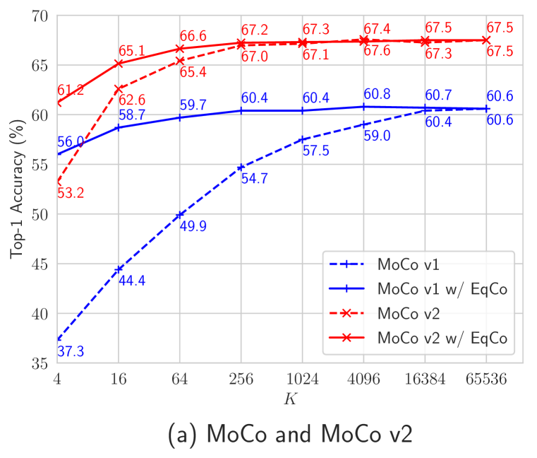
In contrastive learning research, it has been widely believed that enlarging the number of negative samples $K$ boosts the performance ([19, 29, 2]). For example, in MoCo ([17]) the ImageNet accuracy rises from 54.7% to 60.6% under linear classification protocol when $K$ grows from 256 to 65536. Such observation further drives a line of studies how to effectively optimize under a number of negative pairs, such as memory bank methods ([35, 17]) and large batch training ([6]), either of which empirically reports superior performances when $K$ becomes large. Analogously, in the field of supervised metric learning ([11, 32, 28, 34]), loss in the similar form as Eq. 1 is often applied on a lot of negative pairs for hard negative mining. Besides, there are also a few theoretical studies supporting the viewpoint. For instance, [25] points out that the mutual information between the positive pair tends to increase with the number of negative pairs $K$; [33] find that the negative pairs encourage features’ uniformity on the hypersphere; [9] suggests that large $K$ leads to more precise estimation of the debiased contrastive loss; etc.

Despite the above empirical or theoretical evidence, however, we point out that the reason for using many negative pairs is still less convincing. First, unlike the metric learning mentioned above, in self-supervised learning, the negative terms ${\mathbf{k}_{i}}$ in Eq. 1 include both “true negative” (whose underlying class label is different from the query’s, similarly hereinafter) and “false negative” samples, since the actual ground truth label is not available. So, intuitively large K should not always be beneficial because the risk of false negative samples also increases (known as class collision problem). [1] thus theoretically concludes that a large number of negative samples could not necessarily help. Second, some recent works have proven that by introducing new architectures (e.g., a predictor network in BYOL [15]), or designing new loss functions (e.g., [5, 13]), state-of-the-art performance can still be obtained even without any explicit negative pairs. In conclusion, it is still an open question whether large quantities of negative samples are essential to contrastive learning.

After referring to the above two aspects, we rise a question: is a large $K$ really essential in the contrastive learning framework? We propose to rethink the question from a different view: note that in Eq. 1, there are three hyper-parameters: the number of negative samples $K$, temperature $\tau$, and margin $m$. In most of previous empirical studies ([17, 6]), only $K$ is changed while $\tau$ and $m$ are usually kept constant. Do the optimal hyper-parameters of $\tau$ and $m$ varies with $K$? If so, the performance gains observed from larger $K$s may be a wrong interpretation – merely brought by suboptimal hyper-parameters’ choices for small $K$s, rather than much of an essential.

In the paper, we investigate the relationship among three hyper-parameters and suggest an equivalent rule:

$$\footnotesize m=\tau\text{log}\frac{\alpha}{K},$$

where $\alpha$ is a constant. We find that if the margin $m$ is adaptively adjusted based on the above rule, the performance of contrastive learning is irrelevant to the size of $K$, in a very large range (e.g. $K\geq 16$). For example, in MoCo framework, by introducing EqCo the performance gap between $K=256$ and $K=65536$ (the best configuration reported in [17]) almost disappears (from 6.1% decrease to 0.2%). We call this method “Equivalent Rules for Contrastive learning” (EqCo). For completeness, as the other part of EqCo we point that adjusting the learning rate according to the conventional linear scaling rule satisfies the equivalence for different number of queries per batch.

Theoretically, following the InfoMax principle ([23]) and the derivation in CPC ([25]), we prove that in EqCo, the lower bound of the mutual information keeps steady under various numbers of negative samples $K$. Moreover, from the back-propagation perspective, we further prove that in such configuration the upper bound of the gradient norm is also free of $K$’s scale. The proposed equivalent rule implies that, by assigning $\alpha=K_{0}$, it can “mimic” the optimization behavior under $K_{0}$ negative samples even if the physical number of negatives $K\neq K_{0}$.

The “equivalent” methodology of EqCo follows the well-known linear scaling rule ([21, 14]), which suggests scaling the learning rate proportional to the batch size if the loss satisfies with the linear averaged form: $L=\frac{1}{N}\sum_{i=1}^{N}f(x_{i};\theta)$. However, linear scaling rule cannot be directly applied on InfoNCE loss (Eq. 1), which is partially because InfoNCE loss includes two batch sizes (number of queries and keys respectively) while linear scaling rule only involves one, in addition to the nonlinearity of the keys in InfoNCE loss. In the experiments of SimCLR ([6]), learning rates under different batch sizes are adjusted with linear scaling rule, but the accuracy gap is still very large (57.5%@batch=256 vs. 64+%@batch=8192, 100 epochs training).

EqCo challenges the belief that self-supervised contrastive learning requires large quantities of negative pairs to obtain competitive performance, making it possible to design simpler algorithms. We thus present SiMo, a simplified contrastive learning framework based on MoCo v2 ([8]). SiMo is elegant, efficient, free of large batch training and memory bank; moreover, it can achieve superior performances over state-of-the-art even if the number of negative pairs is extremely small (e.g. 16), without bells and whistles.

The contributions of our paper are summarized as follows:

• We challenge the widely accepted belief that on large-scale vision datasets like ImageNet, large size of negative samples is critical for contrastive learning. We interpret it from a different view: it may be because the hyper-parameters are not set to the optimum.

• We propose EqCo, an equivalent rule to adaptively set hyper-parameters between small and large numbers of negative samples, which proves to bridge the performance gap.

• We present SiMo, a simpler but stronger baseline for contrastive learning.

2 EqCo: Equivalent Rules for Contrastive Learning

In this section we introduce EqCo. We mainly consider the circumstance of optimizing the InfoNCE loss (Eq. 1) with SGD. For each batch of training, there are two meanings of the concept “batch size”, i.e., the size of negative samples/pairs $K$ per query, and the number of queries (or positive pairs) $N$ per batch. Hence our equivalent rules accordingly consist of two parts, which will be introduced in the next subsections.

2.1 The Case of Negative Pairs

Our derivation is mainly inspired by the model of Contrastive Predictive Coding (CPC) ([25]), in which InfoNCE loss is interpreted as a mutual information estimator. We further extend the method so that it is applicable to InfoNCE loss with a margin term (Eq. 1), which is not considered in [25].

Following the concept in [25], given a query embedding $\mathbf{q}$ (namely the context in [25]) and suppose $K+1$ random key embeddings $\mathbf{x}=\{\mathbf{x}_{i}\}_{i=0,\dots,K}$, where there exists exactly one entry (e.g., $\mathbf{x}_{i}$) sampled from the conditional distribution $\text{P}(\mathbf{x}_{i}|\mathbf{q})$ while others (e.g., $\mathbf{x}_{j}$) sampled from the “proposal” distribution $\text{P}(\mathbf{x}_{j})$ independently. According to which entry corresponds to the conditional distribution, we therefore defines $K+1$ candidate distributions for $\mathbf{x}$ (denoted by $\{H_{i}\}_{i=0,\dots,K}$), where the probability density of $\mathbf{x}$ under $H_{i}$ is $\text{P}_{H_{i}}(\mathbf{x})=\text{P}(\mathbf{x}_{i}|\mathbf{q})\prod_{j\neq i}\text{P}(\mathbf{x}_{j})$. So, given the observed data $X=\{\mathbf{k}_{0},\dots,\mathbf{k}_{K}\}$ of $\mathbf{x}$, the probability where $\mathbf{x}$ is sampled from $H_{0}$ rather than other candidates is thus derived with Bayes theorem:

$$\text{Pr}[\mathbf{x}\sim H_{0}|\mathbf{q},X] =\frac{\text{P}^{+}\text{P}_{H_{0}}(X)}{\text{P}^{+}\text{P}_{H_{0}}(X)+\text{P}^{-}\sum_{i=1}^{K}\text{P}_{H_{i}}(X)}$$ (2)

$$=\frac{\frac{\text{P}^{+}}{\text{P}^{-}}\frac{\text{P}(\mathbf{k}_{0}|\mathbf{q})}{\text{P}(\mathbf{k}_{0})}}{\frac{\text{P}^{+}}{\text{P}^{-}}\frac{\text{P}(\mathbf{k}_{0}|\mathbf{q})}{\text{P}(\mathbf{k}_{0})}+\sum_{i=1}^{K}\frac{\text{P}(\mathbf{k}_{i}|\mathbf{q})}{\text{P}(\mathbf{k}_{i})}},$$

where we denote $\text{P}^{+}$ and $\text{P}^{-}$ as the prior probabilities of $H_{0}$ and $H_{i}(i>0)$ respectively. We point that Eq. 2 introduces a generalized form to that in [25] by taking the priors into account. Referring to the notations in Eq. 1, we suppose that $H_{0}$ is the ground truth distribution of $\mathbf{x}$ (since $\mathbf{k}_{0}$ is the only positive sample). By modeling the density ratio $\text{P}(\mathbf{k}_{i}|\mathbf{q})/\text{P}(\mathbf{k}_{i})\propto e^{\mathbf{q}^{\top}\mathbf{k}_{i}/\tau}(i=0,\dots,K)$ and letting $\text{P}^{+}/\text{P}^{-}=e^{-m/\tau}$, the negative log-likelihood $\mathcal{L}_{opt}\triangleq\mathbb{E}_{\mathbf{q},X}\ -\text{log}\ \text{Pr}[x\sim H_{0}|\mathbf{q},X]$ can be regarded as the optimal value of $\mathcal{L}_{NCE}$.

Similar to the methodology of [25], we explore the lower bound of $\mathcal{L}_{opt}$:

where $\mathcal{I}(\cdot,\cdot)$ means mutual information. The approximation in the second row is guaranteed by Law of Large Numbers as well as the fact $\text{P}(\mathbf{k}_{i}|\mathbf{q})\approx\text{P}(\mathbf{k}_{i})$ since $\mathbf{k}_{i}(i>0)$ and $\mathbf{q}$ are “almost” independent. The inequality in the last row is resulted from $\text{P}(\mathbf{k}_{0}|\mathbf{q})\geq\text{P}(\mathbf{k}_{0})$ as $\mathbf{k}_{0}$ and $\mathbf{q}$ are extracted from the same instance. Therefore the lower bound of the mutual information (noted as $f_{\text{bound}}(m,K)$) between the positive pair $(\mathbf{k}_{0},\mathbf{q})$ is:

So, minimizing $\mathcal{L}_{NCE}$ (Eq. 1) towards $\mathcal{L}_{opt}$ implies maximizing the lower bound of the mutual information, which is also satisfied when $m\neq 0$. In the case of $m=0$, the result is consistent with that in [25]. [25] further points out the bound increases with $K$, which indicates larger $K$ encourages to learn more mutual information thus could help to improve the performance.

Nevertheless, different from [25] our model does not require $m$ to be zero, so the lower bound in Eq. 4 is also a function of $e^{m/\tau}$. Thus we have the following theorem:

Theorem 1. (Main, EqCo for negative pairs)

The mutual information lower bound of InfoNCE loss in Eq. 1 is irrelevant to the number of negative pairs $K$, if

$$\footnotesize m=\tau\text{log}\frac{\alpha}{K},$$ (5)

where $\alpha$ is a constant coefficient. And in the circumstances the bound is given by:

which can be immediately obtained by substituting Eq. 5 into Eq. 4. We name Eq. 5 as “equivalent condition”.

Theorem 1 suggests a property of equivalency: under the condition of Eq. 5, no matter what the number of physical negative pairs $K$ is, the optimal solution of $\mathcal{L}_{NCE}$ (Eq. 1) is “equivalent” in the sense of the same mutual information lower bound. The bound is controlled by a hyper-parameter $\alpha$ rather than $K$. Eq. 6 further implies that the lower bound also correlates to the configuration of $K=\alpha$ without margin, which suggests we can “mimic” the InfoNCE loss’s behavior of $K=K_{0}$ under a different physical negative sample size $K_{1}$, just by applying Eq. 5 with $\alpha=K_{0}$. It inspires us to simplify the existing state-of-the-art frameworks (e.g. MoCo ([17])) with fewer negative samples but as accurate as the original configurations, which will be introduced next.

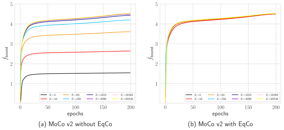
We empirically validate Theorem 1 as follows. Notice that $f_{\text{bound}}$ is difficult to calculate directly because $\mathcal{L}_{opt}$ is not known. Instead, we plot the empirical mutual information lower bound $\hat{f}_{\text{bound}}(m,K)\triangleq\text{log}(1+Ke^{m/\tau})-\mathcal{L}_{NCE}$. So, we have $\hat{f}_{\text{bound}}\leq f_{\text{bound}}$; when $\mathcal{L}_{NCE}$ converges to the optimum $\mathcal{L}_{opt}$, $\hat{f}_{\text{bound}}$ is an approximation of $f_{\text{bound}}$. In Fig. 1, we plot the evolution of $\hat{f}_{\text{bound}}$ during the training of MoCo v2 under different configurations. Obviously, when it converges, without EqCo $\hat{f}_{\text{bound}}$ keeps increasing with the number of negative pairs $K$; in contrast, after applying the equivalent condition (Eq. 5) $\hat{f}_{\text{bound}}$ converges to almost the same value under different $K$s. The empirical results are thus consistent with Theorem 1.

Remarks 1.

The equivalent condition in Eq. 5 suggests the margin $m$ is inversely correlated with $K$. It is intuitive, because the larger $K$ is, the more risks of class collision ([1]) it suffers from, so we need to avoid over-penalty for negative samples near the query, thus smaller $m$ is used; in contrast, if $K$ is very small, we use larger $m$ to exploit more “hard” negative samples.

Besides, recall that the margin term $e^{m/\tau}$ is defined as the ratio of the prior probabilities $\text{P}^{-}/\text{P}^{+}$ in Eq. 2. If the equivalent condition Eq. 5 satisfies, i.e., $\text{P}^{-}/\text{P}^{+}=\alpha/K$, we have $\text{P}^{+}=1/(1+\alpha)$ (notice that $K\text{P}^{-}+\text{P}^{+}\equiv 1$), suggesting that the prior probability of the ground truth distribution $H_{0}$ is supposed to be a constant ignoring the number of negative samples $K$. While in previous works (usually without the margin term, or $m=0$) we have $\text{P}^{+}=1/(K+1)$. It is hard to distinguish which prior is more reasonable. However at least, we intuitively suppose keeping a constant prior for the ground truth distribution may help to keep the optimal choices of hyper-parameters steady under different $K$s, which is also consistent with our empirical observations.

Remarks 2.

In Theorem 1, it is worth noting that $K$ refers to the number of negative samples per query. In the conventional batched training scheme, negative samples for different queries could be either (fully or partially) shared or isolated, i.e., the total number of distinguishing negatives samples per batch could be different, which is not ruled by Theorem 1. However, we empirically find the differences in implementation do not result in much of the performance variation.

Figure 1: Evolution of the empirical mutual information lower bound $\hat{f}_{\text{bound}}$ during training. We use $\alpha=65536$ for EqCo. Results are evaluated with MoCo v2 on ImageNet. Refer to Theorem 1 for details. Best viewed in color.

The following theorem further supports the equivalent rule (Theorem 1) from back-propagation view:

Theorem 2.

Given the equivalent condition (Eq. 5) and a query embedding $\mathbf{q}$ as well as the corresponding positive sample $\mathbf{k}_{0}$, for $\mathcal{L}_{NCE}$ in Eq. 1 the expectation of the gradient norm w.r.t. $\mathbf{q}$ is bounded by :

Please refer to the supplementary materials for the detailed proof. Note that we assume the embedding vectors are normalized, i.e., $\left\|\mathbf{k}_{i}\right\|=1(i=0,\cdots,K)$, which is also a convention in recent contrastive learning works.

(a) @50 epochs

(b) @100 epochs

(c) @150 epochs

(d) @200 epochs

Figure 2: The means (solid line) and variances (ribbon, $\pm 2\sigma$) of $\left\|\mathrm{d}\mathcal{L}_{NCE}/\mathrm{d}\bm{q}\right\|$ under different $K$s. We train a normal MoCo v2 for 200 epochs and show the statistics at different epochs.

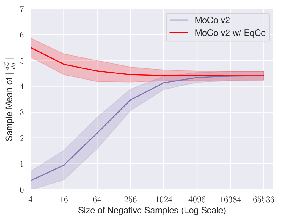
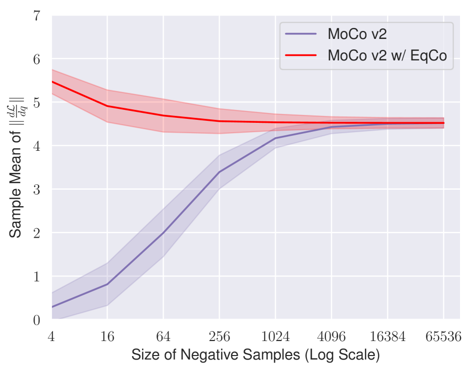
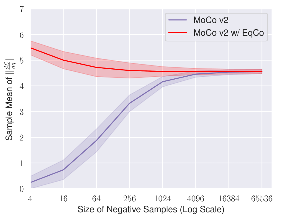
Theorem 2 indicates that, equipped with the equivalent rule (Eq. 5), the upper bound of the gradient norm is irrelevant to the number of negative samples $K$. Fig. 2 further validates our theory: the gradient norm becomes much more steady after using EqCo under different $K$s. Since the size of $K$ affects little on the gradient magnitude, gradient scaling techniques, e.g. linear scaling rule, are not required specifically for different $K$s. Eq. 7 also implies that the temperature $\tau$ significantly affects the gradient norm even EqCo is applied – it is why we only recommend to modify $m$ for equivalence (Eq. 5), though the mutual information lower bound is determined by $e^{m/\tau}$ as a whole.

2.2 The Case of Positive Pairs

In practice the InfoNCE loss (Eq. 1) is usually optimized with batched SGD, which can be represented as empirical risk minimization:

$$\footnotesize\mathcal{L}_{NCE}^{\text{batch}}=\frac{1}{N}\sum_{j=1}^{N}\mathcal{L}_{NCE}^{(j)}(\mathbf{q}_{j},\mathbf{k}_{j,0}),$$ (8)

where $N$ is the number of queries (or positive pairs) per batch; $(\mathbf{q}_{j},\mathbf{k}_{j,0})\sim(\mathcal{D},\mathcal{D}^{\prime}(\mathbf{q}_{j}))$ is the $j$-th positive pair, and $\mathcal{L}_{NCE}^{(j)}(\mathbf{q}_{j},\mathbf{k}_{j,0})$ is the corresponding loss. For different $j$, $\mathcal{L}_{NCE}^{(j)}$ is (almost) independent of each other, because $\mathbf{q}_{j}$ is sampled independently. Hence, Eq. 8 satisfies the form of linear scaling rule ([21, 14]), suggesting that the learning rate should be adjusted proportional to the number of queries $N$ per batch.

Remarks 3.

Previous work like SimCLR ([6]) also proposes to apply linear scaling rule. The difference is, in SimCLR it does not clarify the concept of “batch size” refers to the number of queries or the number of keys. However in our paper, we explicitly point that the linear scaling rule needs to be applied corresponding to the number of queries per batch ($N$) rather than $K$.

2.3 Empirical Evaluation

In this subsection we conduct experiments using cvpods [38] (based on PyTorch) on three state-of-the-art self-supervised contrastive learning frameworks – MoCo ([17]), MoCo v2 ([8]) and SimCLR ([6]) to verify our theory in Sec. 2.1 and Sec. 2.2. We propose to alter $K$ and $N$ separately to examine the correctness of our equivalent rules.

Implementation details.

We follow most of the training and evaluation settings recommended in the original papers respectively. The only difference is, for SimCLR, we adopt SGD with momentum rather than LARS ([37]) as the optimizer. We use ResNet-50 ([18]) as the default network architecture. 128-d features are employed for query and key embeddings. Unless specially mentioned, all models are trained on ImageNet ([10]) for 200 epochs without using the ground truth labels. We report the top-1 accuracy under the conventional linear evaluation protocol according to the original paper respectively. The number of queries per batch ($N$) is set to 256 by default. All models are trained with 8 GPUs.

It is worth noting the way we alter the number of negative samples $K$ independent of $N$ during training. For MoCo and MoCo v2, we simply need to set the size of the memory bank to $K$. Specially, if $K<N$, in the current batch the memory bank is actually composed of $K$ random keys sampled from the previous batch. While for SimCLR, if $K<N$ we random sample $K$ negative keys for each query independently. We do not study the case that $K>N$ for SimCLR. We mainly consider the ease of implementation in designing the strategies; as mentioned in Remarks 2 (Sec. 2.1), it does not affect the empirical conclusion.

Quantitative results.

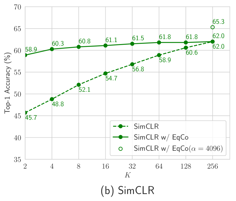
Fig. 3 illustrates the effect of our equivalent rule under different $K$s. Our experiments start with the best configurations (i.e. $K=65536$ for MoCo and MoCo v2, and $K=256$ for SimCLR), then we gradually reduce $K$ and benchmark the performance. Results in Fig. 3 indicates that, without EqCo the accuracy significantly drops if $K$ becomes very small (e.g. $K<64$). While with EqCo, by setting $\alpha$ to “mimic” the optimal $K$, the performance surprisingly keeps steady under a wide range of $K$s. Fig. 3(b) further shows that in SimCLR, by setting $\alpha$ to a number larger than the physical batch size (e.g. 4096 vs. 256), the accuracy significantly improves from 62.0% to 65.3%, suggesting the benefit of EqCo especially when the memory is limited. The comparison fully demonstrates EqCo is essential especially when the number of negative pairs is small.

Figure 3: Comparisons with/without EqCo under different number of negative samples (noted by $K$). Results are evaluated with ImageNet top-1 accuracy using linear evaluation protocol. In EqCo, we set $\alpha=65536$ for MoCo and MoCo v2, and $\alpha=256$ for SimCLR (except for one data point with $\alpha=4096$, as noted in the legend). Best viewed in color.

Besides, Table 1 compares the results of MoCo v2 under different number of queries $N$, while $K=65536$ is fixed. It is clear that, with linear scaling rule ([21, 14]), the final performance is almost unchanged under different $N$, suggesting the effectiveness of our equivalent rule for $N$.

$N(K=65536)$	256	512	1024
Top-1 accuracy (%)	67.5	67.5	67.4

Table 1: ImageNet accuracy (MoCo v2) vs. the number of queries per batch ($N$). The learning rates during training are adjusted with linear scaling rule.

3 A Simpler but Stronger Baseline

EqCo inspires us to rethink the design of contrastive learning frameworks. The previous state-of-the-arts like MoCo and SimCLR heavily rely on large quantities of negative pairs to obtain high performances, hence implementation tricks such as memory bank and large batch training are introduced, which makes the system complex and tends to be costly. Thanks to EqCo, we are able to design a simpler contrastive learning framework with fewer negative pairs.

Figure 4: SiMo with/without EqCo

Method	Epochs	Top-1 (%)
CPC v2 [19]	200	63.8
CMC [29]	240	66.2
SimCLR [6]	200	66.6
MoCo v2 [8]	200	67.5
InfoMin Aug. ([30])	200	70.1
SiMo ($K=16,\alpha=256$)	200	68.1
SiMo ($K=256,\alpha=256$)	200	68.0
SiMo ($K=256,\alpha=65536$)	200	68.5
PIRL [24]	800	63.6
SimCLR [6]	1000	69.3
MoCo v2 [8]	800	71.1
InfoMin Aug. ([30])	800	73.0
SiMo ($K=256,\alpha=256$)	800	71.8
SiMo ($K=256,\alpha=65536$)	800	72.1

Table 2: State-of-the-art InfoNCE-based frameworks

We propose SiMo, a simplified variant of MoCo v2 ([8]) equipped with EqCo. We follow most of the design in [8], where the key differences are as follows:

Memory bank.

MoCo, MoCo v2 and SimCLR v2 ([7]) employ memory bank to maintain large number of negative embeddings $\mathbf{k}_{i}$, in which there is a side effect: every positive embedding $\mathbf{k}_{0}$ is always extracted from a “newer” network than the negatives’ in the same batch, which could harm the performance. In SiMo, we thus cancel the memory bank as we only rely on a few negative samples per batch. Instead, we use the momentum encoder to extract both positive and negative $key$ embeddings from the current batch.

Shuffling BN vs. Sync BN. In MoCo v1/v2, shuffling BN ([17]) is proposed to remove the obvious dissimilarities of the BN ([20]) statistics between the positive (from current mini-batch) and the negatives (from memory bank), so that the model can make predictions based on the semantic information of images rather than the BN statistics. In contrast, since the positive and negatives are from the same batch in SiMo, therefore, we use sync BN ([26]) for simplicity and more stable statistics. Sync BN is also used in SimCLR ([6]) and SimCLR v2 ([7]).

There are a few other differences, including 1) we use a BN attached to each of the fully-connected layers; 2) we introduce a warm-up stage at the beginning of the training, which follows the methodology in SimCLR ([6]). Apart from all the differences mentioned above, the architecture and the training (including data augmentations) details in SiMo are exactly the same as MoCo v2’s. In the following text, the number of queries per batch (N) is set to 256, and the backbone network is ResNet-50 by default.

Quantitative results.

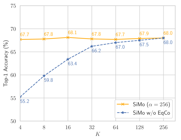
First, we empirically demonstrate the necessity of EqCo in SiMo framework. We choose the number of negative samples $K=256$ as the baseline, then reduce $K$ to evaluate the performance. Fig. 4 shows the result on ImageNet using linear evaluation protocol. Without EqCo, the accuracy significantly drops when $K$ is very small. In contrast, using EqCo to “mimic” the case of large $K$ (by setting $\alpha$ to 256), the accuracy almost keeps steady even under very small $K$s.

Table 2 further compares our SiMo with state-of-the-art self-supervised contrastive learning methods on ImageNet. Using only 16 negative samples per query, SiMo outperforms MoCo v2 (68.1% vs. 67.5%). If we increase $\alpha$ to 65536 to “simulate” the case under huge number of negative pairs, the accuracy further increases to 68.5%. Moreover, when we extend the training epochs to 800, we get the accuracy of 72.1%, surpassing the baseline MoCo v2 by 1.0%. The only entry that surpasses our results is InfoMin Aug. ([30]), which is mainly focuses on data generation and orthogonal to ours.

As shown in Sec.2.1, $\alpha$ is related to the lower bound of mutual information. Table 3 reveals how accuracy of SiMo varies with the choice of $\alpha$. As we increase $\alpha$ to 65536, the accuracy tends to improve, in accordance with the Eq.6.

$\alpha$	256	1024	4096	16384	65536
Accuracy (%)	68.0	68.1	68.1	68.4	68.5

Table 3: SiMo with different $\alpha$.

Similar results can be found in MoCo v2. We increase $K$ to 65536 in MoCo v2, the accuracy also descends (in Table 4).

$K$	256	1024	4096	16384	65536
Accuracy (%)	67.0	67.1	67.6	67.3	67.5

Table 4: MoCo v2 with different $K$.

The experiments indicate that SiMo is a simpler but more powerful baseline for self-supervised contrastive learning. Readers can refer to the Supplementary for more experimental results of SiMo.

A Toy Evaluation of EqCo.

To evaluate the effectiveness of EqCo as mutual information (MI) estimator, following the configuration of [27], we estimate the MI lower bound of between two simple random vectors.

Specifically, given that $\left(X,Y\right)$ are drawn from the known correlated Gaussian distribution, we calculate the lower bound of MI between $X$ and $Y$ based on their embedding. $X$ is a 20-dimensional random variables drawn from a standard Gaussian distribution. And we sampled $Y$ with the following rule:

$$\footnotesize Y=\rho X+\sqrt{1-{\rho}^{2}}\ \epsilon$$ (9)

where $\rho$ is a the given correlation coefficient and $\epsilon$ is a random variable sampled from a standard Gaussian distribution and independent from $X$. With a known $\rho$, the ground truth MI between $X$ and $Y$ is easy to compute:

$$\footnotesize\mathcal{I}\left(X,Y\right)=-\frac{d}{2}\log\left(1-{\rho}^{2}\right)$$ (10)

Here, $d$ is the dimension of $X$ and $Y$, and as mentioned above we set $d=20$.

To embed $X$ and $Y$, we adopt two MLPs respectively, and each MLP has 1 hidden layer of 256 units, followed by ReLU activation function. We use Adam optimizer with learning rate of 0.0005 to optimize InfoNCE or EqCo for 5000 steps. For each training iteration, $K$ pairs of $\left(X,Y\right)$ are independently sampled, which means there are $K-1$ negative samples for each query. After training, the weights of MLPs are frozen and we repeat estimating the lower bound of MI for 1000 times to reduce the estimating variance. For experiments with EqCo, we set the $\alpha=512$.

As shown in Table 5, $\mathcal{I}_{NCE}$ varies with $K$, while $\mathcal{I}_{EqCo}$ remains steady. Especially, when the ground truth MI is relatively large (e.g., 8, 10), significant differences between EqCo and InfoNCE can be observed. The experiment further validates the effectiveness of EqCo.

	$K$
	64	128	256	512
Mutual Information$\ =2.0$
$\mathcal{I}_{NCE}$	1.7	1.8	1.9	1.9
$\mathcal{I}_{EqCo}$	1.9	1.9	1.9	1.9
Mutual Information$\ =4.0$
$\mathcal{I}_{NCE}$	2.9	3.2	3.4	3.6
$\mathcal{I}_{EqCo}$	3.8	3.7	3.6	3.6
Mutual Information$\ =6.0$
$\mathcal{I}_{NCE}$	3.6	4.1	4.5	4.9
$\mathcal{I}_{EqCo}$	5.1	5.0	4.9	4.9
Mutual Information$\ =8.0$
$\mathcal{I}_{NCE}$	3.9	4.6	5.1	5.6
$\mathcal{I}_{EqCo}$	5.8	5.7	5.7	5.6
Mutual Information$\ =10.0$
$\mathcal{I}_{NCE}$	4.1	4.7	5.4	6.0
$\mathcal{I}_{EqCo}$	6.1	6.0	6.0	6.0

Table 5: Estimating mutual information by InfoNCE and EqCo with different batch size and various ground truth mutual information.

4 Limitations and Future Work

Theorem 1 suggests that given the equivalent condition (Eq. 5), InfoNCE losses under various $K$s are “equivalent” in the sense of the same mutual information lower bound, which is also backed up with the experiments in Fig. 1. However, Fig. 3 (a) shows that if $K$ is smaller than a certain value (e.g. $K\leq 16$), some frameworks like MoCo v2 start to degrade significantly even with EqCo; while for other frameworks like SiMo (Fig. 4), the accuracy almost keeps steady for very small $K$s. [31] also point that the principle of InfoMax cannot explain all the phenomena in contrastive learning. We will investigate the problem in the future, e.g. from other viewpoints such as gradient noise brought by small $K$s (Fig. 2 gives some insights).

Though the formulation of Eq. 1 is very common in the field of supervised metric learning, which is usually named margin softmax cross-entropy loss [11, 32, 28]. Nevertheless, unfortunately, our equivalent rule seems invalid to be generalized to those problems (e.g. face recognition). The major issue lies in the approximation in Eq. 3, we need the negative samples $\mathbf{k}_{i}$ to be independent of the query $\mathbf{q}$, which is not satisfied in supervised tasks.

According to Fig. 3 and Fig. 4, the benefits of EqCo become significant if $K$ is sufficiently small (e.g. $K<64$). But in practice, for modern computing devices (e.g. GPUs) it is not that difficult to use $\sim 256$ negative pairs per query. Applying EqCo to “simulate” more negative pairs via adjusting $\alpha$ can further boost the performance, however, whose accuracy gains become relatively marginal. For example, in Table 2 under 200 epochs training, SiMo with $\alpha=65536$ outperforms that of $\alpha=256$ by only 0.5%. It could be a fundamental limitation of InfoNCE loss. We will investigate the problem in the future.

Appendix A Details about Theorem 2

A.1 Proof of Eq. 7

Given the equivalent condition (Eq. 5) and a query embedding $\mathbf{q}$ as well as the corresponding positive sample $\mathbf{k}_{0}$, for $\mathcal{L}_{NCE}$ in Eq. 1 the expectation of the gradient norm w.r.t. $\mathbf{q}$ is bounded by:

Proof. For simplicity, we denote the term $\exp(\mathbf{q}^{\top}\mathbf{k}_{i}/\tau)$ as $s_{i}(i=0,\dots,K)$. Then $\mathcal{L}_{NCE}$ can be rewritten as:

$$\footnotesize\mathcal{L}_{NCE}=-\log\frac{s_{0}}{s_{0}+\frac{\alpha}{K}\sum_{i=1}^{K}s_{i}}$$ (12)

The gradient of $\mathcal{L}_{NCE}$ with respect to $\mathbf{q}$ is easily to derived:

Owing to the Triangle Inequality and the fact that $\mathbf{k}_{i}(i=0,\dots,K)$ is normalized, the norm of gradient is bounded by:

Since the cosine similarity between $\mathbf{q}\text{ and }\mathbf{k}_{i}\left(i=1,\dots,K\right)$ is bounded in $\left[-1,1\right]$, we know the expectation of $\mathop{\mathbb{E}}_{\mathbf{k}_{i}\sim\mathcal{D}^{\prime}}\left[s_{i}\right]$ exists. According to Inequality (14) and Jensen’s Inequality, we have:

Replacing $s_{i}$ by $\exp(\mathbf{q}^{\top}\mathbf{k}_{i}/\tau)$, the proof of Theorem 2 is completed.

Appendix B More Experiments on SiMo

For the following experiments of this section, we report the top-1 accuracy of SiMo on ImageNet [10] under the linear evaluation protocol. The backbone of SiMo is ResNet-50 [18] and we train SiMo for 200 epochs unless noted otherwise.

B.1 Ablation on Momentum Update

In MoCo [17] and MoCo v2 [8], the key encoder is updated by the following rule:

$$\footnotesize{\theta}_{k}=\beta{\theta}_{k}+\left(1-\beta\right){\theta}_{q}$$ (16)

where ${\theta}_{q}\text{ and }{{\theta}_{k}}$ stand for the weights of query encoder and key encoder respectively, and $\beta$ is the momentum coefficient. For SiMo, we also adopt the momentum update and use the key encoder to compute the features of positive sample and negative samples.

In Table 6, we report the results of SiMo with different momentum coefficients. The number of training epochs is set to be 100, so the top-1 accuracy of baseline ($\beta=0.999$) drops to 64.4%. Compared to the baseline, SiMo without momentum update ($\beta=0$) is inferior, showing the advantage of momentum update.

$\beta$	0	0.999
Accuracy (%)	62.1	64.4

Table 6: Ablation on momentum update.

B.2 Ablation on BN

Table 7 shows the performance of SiMo equipped with shuffling BN or Sync BN. Likewise, we train SiMo for 100 epochs. It is easy to check out that SiMo with shuffling BN struggles to perform well. Besides, compared to MoCo v2, SiMo with shuffling BN degrades significantly, and we conjecture that it is because the MLP structure of SiMo is more suitable for Sync BN, rather than shuffling BN.

	Shuffling BN	Sync BN
Accuracy (%)	58.8	64.4

Table 7: Sync BN vs. shuffling BN.

B.3 SiMo with Wider Models

Results using wider models are presented in Table 8. For SiMo, the performance is further boosted with wider models (more channels). For instance, SiMo with ResNet-50 (2x) and ResNet-50 (4x) outperforms the baseline (68.5%) by 2% and 3.8% respectively.

Architecture	Param. (M)	$\alpha$	Top-1 (%)
ResNet-50 (2x)	94	256	70.2
ResNet-50 (2x)	94	65536	70.5
ResNet-50 (4x)	375	256	71.9
ResNet-50 (4x)	375	65536	72.3

Table 8: SiMo with wider models. All models are trained with 200 epochs.

B.4 Transfer to object detection

Setup

We utilize FPN [22] with a stack of 4 $3\times 3$ convolution layers in R-CNN head to validate the effectiveness of SiMo. Following the MoCo training protocol, we fine-tune with synchronized batch-normalization [26] across GPUs. The additional initialized layers are also equipped with BN for stable training. To effectively validate the transferability of the features, the training schedule is set to be 12 epochs (known as 1$\times$), in which learning rate is initialized as 0.2 and decreased at 7 and 11 epochs with a factor of 0.1. The image scales are random sampled of $\left[640,800\right]$ pixels during training and fixed with 800 at inference.

Results

Table 9 summarizes the fine-tuning results on COCO val2017 of different pre-training methods. Random initialization indicates training COCO from scratch, and supervised represents conventional pre-training with ImageNet labels. Compared with MoCo, SiMo achieves competitive performance without large quantities of negative pairs. It is also on a par with the supervised counterpart and significantly outperforms random initialized one.

Table 9: Object detection fine-tuned on COCO.

pre-train	AP	AP50	AP75	APs	APm	APl
random init	31.4	49.4	34.0	17.9	32.3	41.6
supervised	39.0	59.1	42.6	22.4	42.2	50.6
MoCo v2	39.1	59.2	42.5	23.3	42.1	50.8
SiMo	39.0	59.2	42.3	22.9	41.8	50.5

References

- [1] Sanjeev Arora, Hrishikesh Khandeparkar, Mikhail Khodak, Orestis Plevrakis, and Nikunj Saunshi. A theoretical analysis of contrastive unsupervised representation learning. arXiv preprint arXiv:1902.09229, 2019.
- [2] Philip Bachman, R Devon Hjelm, and William Buchwalter. Learning representations by maximizing mutual information across views. In Advances in Neural Information Processing Systems, pages 15535–15545, 2019.
- [3] Yue Cao, Zhenda Xie, Bin Liu, Yutong Lin, Zheng Zhang, and Han Hu. Parametric instance classification for unsupervised visual feature learning. arXiv preprint arXiv:2006.14618, 2020.
- [4] Mathilde Caron, Ishan Misra, Julien Mairal, Priya Goyal, Piotr Bojanowski, and Armand Joulin. Unsupervised learning of visual features by contrasting cluster assignments. Advances in Neural Information Processing Systems, 33, 2020.
- [5] Mathilde Caron, Ishan Misra, Julien Mairal, Priya Goyal, Piotr Bojanowski, and Armand Joulin. Unsupervised learning of visual features by contrasting cluster assignments. arXiv preprint arXiv:2006.09882, 2020.
- [6] Ting Chen, Simon Kornblith, Mohammad Norouzi, and Geoffrey Hinton. A simple framework for contrastive learning of visual representations. arXiv preprint arXiv:2002.05709, 2020.
- [7] Ting Chen, Simon Kornblith, Kevin Swersky, Mohammad Norouzi, and Geoffrey E Hinton. Big self-supervised models are strong semi-supervised learners. Advances in Neural Information Processing Systems, 33, 2020.
- [8] Xinlei Chen, Haoqi Fan, Ross Girshick, and Kaiming He. Improved baselines with momentum contrastive learning. arXiv preprint arXiv:2003.04297, 2020.
- [9] Ching-Yao Chuang, Joshua Robinson, Lin Yen-Chen, Antonio Torralba, and Stefanie Jegelka. Debiased contrastive learning. arXiv preprint arXiv:2007.00224, 2020.
- [10] Jia Deng, Wei Dong, Richard Socher, Li-Jia Li, Kai Li, and Li Fei-Fei. Imagenet: A large-scale hierarchical image database. In 2009 IEEE conference on computer vision and pattern recognition, pages 248–255. Ieee, 2009.
- [11] Jiankang Deng, Jia Guo, Niannan Xue, and Stefanos Zafeiriou. Arcface: Additive angular margin loss for deep face recognition. In Proceedings of the IEEE Conference on Computer Vision and Pattern Recognition, pages 4690–4699, 2019.
- [12] Alexey Dosovitskiy, Jost Tobias Springenberg, Martin Riedmiller, and Thomas Brox. Discriminative unsupervised feature learning with convolutional neural networks. In Advances in neural information processing systems, pages 766–774, 2014.
- [13] Aleksandr Ermolov, Aliaksandr Siarohin, Enver Sangineto, and Nicu Sebe. Whitening for self-supervised representation learning. arXiv preprint arXiv:2007.06346, 2020.
- [14] Priya Goyal, Piotr Dollár, Ross Girshick, Pieter Noordhuis, Lukasz Wesolowski, Aapo Kyrola, Andrew Tulloch, Yangqing Jia, and Kaiming He. Accurate, large minibatch sgd: Training imagenet in 1 hour. arXiv preprint arXiv:1706.02677, 2017.
- [15] Jean-Bastien Grill, Florian Strub, Florent Altché, Corentin Tallec, Pierre H Richemond, Elena Buchatskaya, Carl Doersch, Bernardo Avila Pires, Zhaohan Daniel Guo, Mohammad Gheshlaghi Azar, et al. Bootstrap your own latent: A new approach to self-supervised learning. arXiv preprint arXiv:2006.07733, 2020.
- [16] Raia Hadsell, Sumit Chopra, and Yann LeCun. Dimensionality reduction by learning an invariant mapping. In 2006 IEEE Computer Society Conference on Computer Vision and Pattern Recognition (CVPR’06), volume 2, pages 1735–1742. IEEE, 2006.
- [17] Kaiming He, Haoqi Fan, Yuxin Wu, Saining Xie, and Ross Girshick. Momentum contrast for unsupervised visual representation learning. In Proceedings of the IEEE/CVF Conference on Computer Vision and Pattern Recognition, pages 9729–9738, 2020.
- [18] Kaiming He, Xiangyu Zhang, Shaoqing Ren, and Jian Sun. Deep residual learning for image recognition. In Proceedings of the IEEE conference on computer vision and pattern recognition, pages 770–778, 2016.
- [19] Olivier J Hénaff, Aravind Srinivas, Jeffrey De Fauw, Ali Razavi, Carl Doersch, SM Eslami, and Aaron van den Oord. Data-efficient image recognition with contrastive predictive coding. arXiv preprint arXiv:1905.09272, 2019.
- [20] Sergey Ioffe and Christian Szegedy. Batch normalization: Accelerating deep network training by reducing internal covariate shift. arXiv preprint arXiv:1502.03167, 2015.
- [21] Alex Krizhevsky. One weird trick for parallelizing convolutional neural networks. arXiv preprint arXiv:1404.5997, 2014.
- [22] Tsung-Yi Lin, Piotr Dollár, Ross Girshick, Kaiming He, Bharath Hariharan, and Serge Belongie. Feature pyramid networks for object detection. In Proceedings of the IEEE conference on computer vision and pattern recognition, pages 2117–2125, 2017.
- [23] Ralph Linsker. Self-organization in a perceptual network. Computer, 21(3):105–117, 1988.
- [24] Ishan Misra and Laurens van der Maaten. Self-supervised learning of pretext-invariant representations. In Proceedings of the IEEE/CVF Conference on Computer Vision and Pattern Recognition, pages 6707–6717, 2020.
- [25] Aaron van den Oord, Yazhe Li, and Oriol Vinyals. Representation learning with contrastive predictive coding. arXiv preprint arXiv:1807.03748, 2018.
- [26] Chao Peng, Tete Xiao, Zeming Li, Yuning Jiang, Xiangyu Zhang, Kai Jia, Gang Yu, and Jian Sun. Megdet: A large mini-batch object detector. In Proceedings of the IEEE Conference on Computer Vision and Pattern Recognition, pages 6181–6189, 2018.
- [27] Ben Poole, Sherjil Ozair, Aaron van den Oord, Alexander A Alemi, and George Tucker. On variational bounds of mutual information. arXiv preprint arXiv:1905.06922, 2019.
- [28] Yifan Sun, Changmao Cheng, Yuhan Zhang, Chi Zhang, Liang Zheng, Zhongdao Wang, and Yichen Wei. Circle loss: A unified perspective of pair similarity optimization. In Proceedings of the IEEE/CVF Conference on Computer Vision and Pattern Recognition, pages 6398–6407, 2020.
- [29] Yonglong Tian, Dilip Krishnan, and Phillip Isola. Contrastive multiview coding. arXiv preprint arXiv:1906.05849, 2019.
- [30] Yonglong Tian, Chen Sun, Ben Poole, Dilip Krishnan, Cordelia Schmid, and Phillip Isola. What makes for good views for contrastive learning. arXiv preprint arXiv:2005.10243, 2020.
- [31] Michael Tschannen, Josip Djolonga, Paul K Rubenstein, Sylvain Gelly, and Mario Lucic. On mutual information maximization for representation learning. arXiv preprint arXiv:1907.13625, 2019.
- [32] Hao Wang, Yitong Wang, Zheng Zhou, Xing Ji, Dihong Gong, Jingchao Zhou, Zhifeng Li, and Wei Liu. Cosface: Large margin cosine loss for deep face recognition. In Proceedings of the IEEE Conference on Computer Vision and Pattern Recognition, pages 5265–5274, 2018.
- [33] Tongzhou Wang and Phillip Isola. Understanding contrastive representation learning through alignment and uniformity on the hypersphere. arXiv preprint arXiv:2005.10242, 2020.
- [34] Xun Wang, Haozhi Zhang, Weilin Huang, and Matthew R Scott. Cross-batch memory for embedding learning. In Proceedings of the IEEE/CVF Conference on Computer Vision and Pattern Recognition, pages 6388–6397, 2020.
- [35] Zhirong Wu, Yuanjun Xiong, Stella X Yu, and Dahua Lin. Unsupervised feature learning via non-parametric instance discrimination. In Proceedings of the IEEE Conference on Computer Vision and Pattern Recognition, pages 3733–3742, 2018.
- [36] Jiahao Xie, Xiaohang Zhan, Ziwei Liu, Yew Soon Ong, and Chen Change Loy. Delving into inter-image invariance for unsupervised visual representations. arXiv preprint arXiv:2008.11702, 2020.
- [37] Yang You, Igor Gitman, and Boris Ginsburg. Large batch training of convolutional networks. arXiv preprint arXiv:1708.03888, 2017.
- [38] Benjin Zhu, Feng Wang, Jianfeng Wang, Siwei Yang, Jianhu Chen, and Zeming Li. cvpods: All-in-one toolbox for computer vision research, 2020.