Local Label Point Correction for Edge Detection of Overlapping Cervical Cells

Abstract

Accurate labeling is essential for supervised deep learning methods. However, it is almost impossible to accurately and manually annotate thousands of images, which results in many labeling errors for most datasets. We proposes a local label point correction (LLPC) method to improve annotation quality for edge detection and image segmentation tasks. Our algorithm contains three steps: gradient-guided point correction, point interpolation and local point smoothing. We correct the labels of object contours by moving the annotated points to the pixel gradient peaks. This can improve the edge localization accuracy, but it also causes unsmooth contours due to the interference of image noise. Therefore, we design a point smoothing method based on local linear fitting to smooth the corrected edge. To verify the effectiveness of our LLPC, we construct a largest overlapping cervical cell edge detection dataset (CCEDD) with higher precision label corrected by our label correction method. Our LLPC only needs to set three parameters, but yields 30-40$\%$ average precision improvement on multiple networks. The qualitative and quantitative experimental results show that our LLPC can improve the quality of manual labels and the accuracy of overlapping cell edge detection. We hope that our study will give a strong boost to the development of the label correction for edge detection and image segmentation. We will release the dataset and code at https://github.com/nachifur/LLPC.

Corresponding author: Huijie Fan, Danbo Wang

Keywords: label correction, point correction, edge detection, segmentation, local point smoothing, cervical cell dataset

1 Introduction

Medical image datasets are generally annotated by professional physicians [1, 2, 3, 4, 5, 6, 7]. To construct an annotated dataset for edge detection or image segmentation tasks, annotators often need to annotate points and connect them into an object outline. In the manual labeling process, it is difficult to control label accuracy due to human error. Northcutt et al. found that label errors are numerous and universal: the average error rate in 10 datasets is 3.4$\%$ [8]. These wrong labels seriously affect the accuracy of model evaluation and destabilize benchmarks, which will ultimately spill over model selection and deployment. For example, the deployed model in learning-based computer-aided diagnosis [9, 10, 11, 12, 13] is selected from many candidate models based on evaluation accuracy, which means that inaccurate annotations may ultimately affect accurate diagnosis. To mitigate labeling errors, an image is often annotated by multiple annotators [2, 4, 14], which generates multiple labels for one image. However, even if the annotation standard is unified, differences between different annotators are inevitable. Another way is to correct the labels manually [5]. In fact, multi-person annotation and manual label correction are time-consuming and labor-intensive. Therefore, it is of great value to develop label correction methods based on manual annotation for supervised deep learning methods.

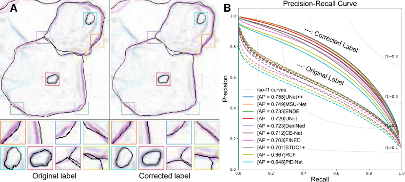
Most label correction works are focused on weak supervision [15], semi-supervision [16], crowdsourced labeling [17, 18], classification [19, 20, 21, 22, 23, 24] and natural language processing [25]. However, label correction in these tasks is completely different from correcting object contours. To automatically correct edge labels, we propose a local label point correction method for edge detection and image segmentation. Our method contains three steps: gradient-guided point correction, point interpolation and local point smoothing. We correct the annotation of the object contours by moving label points to the pixel gradient peaks and smoothing the edges formed by these points. To verify the effectiveness of our label correction method, we construct a cervical cell edge detection dataset. Experiments with multiple state-of-the-art deep learning models on the CCEDD show that our LLPC can greatly improve the quality of manual annotation and the accuracy of overlapping cell edge detection, as shown in Figure 1. Our unique contributions are summarized as follows:

• We are the first to propose a label correction method based on annotation points for edge detection and image segmentation. By correcting the position of these label points, our label correction method can generate higher-quality label, which contributes 30-40$\%$ AP improvement on multiple baseline models.

• We construct a largest publicly cervical cell edge detection dataset based on our LLPC. Our dataset is ten times larger than the previous datasets, which greatly facilitates the development of overlapping cell edge detection.

• We present the first publicly available label correction benchmark for improving contour annotation. Our study serves as a potential catalyst to promote label correction research and further paves the way to construct accurately annotated datasets for edge detection and image segmentation.

Figure 1: (A) Visual comparison of the original label and our corrected label. Our LLPC can improve the edge positioning accuracy and generate more accurate edge labels. (B) Precision-Recall curves of edge detection methods on our CCEDD dataset. The average precision (AP) is significantly improved over multiple baseline models by using our corrected labels.

2 RELATED WORK

Label Correction. Deep learning is developing rapidly with the help of big computing [26] and big data [27, 28, 29]. Some works [30, 31, 32] focus on feeding larger models with more data for better performance and generalization, while others design task-specific model structures and loss functions [33, 34, 35] to improve performance on a fixed dataset. Recently, data itself has received a lot of attention. Andrew Ng et al. [36] led the data revolution of deep learning and successfully organized the first ”Data-Centric AI” competition. The competition aims to improve data quality and develop data optimization pipelines, such as label correction, data synthesis and data augmentation [37]. Competitors mine data potential instead of optimizing model structure to improve performance. Northcutt et al. [8] found that if the error rate of test labels only increases by 6$\%$, ResNet18 outperforms ResNet-50 on ImageNet [27]. To improve data quality and accurately evaluate models, there is an urgent need to develop label correction algorithms. In weak supervision and semi-supervision [15, 16], pseudo label correction is usually implemented due to the lack of supervision from real labels. Zheng et al. [15] correct the noisy labels by using a meta network for image recognition and text classification. For supervised learning, bad data can be discarded by data preprocessing, but bad labels seem inevitable in large-scale datasets. In crowdsourcing [17, 18], an image is annotated by multiple people to improve the accuracy of classification task [19, 20, 21]. Guo et al. [21] trained a model by using a small amount of data and design a label completion method to generate labels (negative or positive) for the mostly unlabeled data. However, label correction in these tasks is significantly different from correcting object contours. In this paper, to eliminate edge location errors and inter-annotator differences in manual annotation, we propose an label correction method based on annotation points for edge detection and image segmentation. Besides, we compare our LLPC with conditional random fields (CRF) [38], which is popular as post-processing for other segmentation methods [39, 40, 41, 42, 43, 44]. Dense CRF [45] improves the labeling accuracy by optimizing energy function based on coarse segmentation images, while our LLPC is a label correction method based on annotation points, which are two different technical routes of label correction for image segmentation. More discussion in Section 5.3.

Cervical Cell Dataset. Currently, cervical cell datasets include ISBI 2015 challenge dataset [46], Shenzhen University dataset [47] and Beihang University dataset [11]. Supervised deep learning based methods require large amounts of data with accurate annotations. However, the only public ISBI dataset [46] has a small amount of data and simple image types, which are difficult to train deep neural networks. In this paper, we construct a largest high-accuracy cervical cell edge detection dataset based on our label correction method. Our CCEDD contains overlapping cervical cell masses in a variety of complex backgrounds and high-precision corrected labels, which are sufficient in quantity and richness to train various deep learning models.

3 Label Correction

Our LLPC contains three steps: gradient-guided point correction (GPC), point interpolation (PI) and local point smoothing (LPS). $I(x,y)$ is a cervical cell image and $g(x,y)$ is the gradient image of $I(x,y)$ after Gaussian smoothing. $x_{s}^{i}$ is an original label point of $I(x,y)$. First, we correct the points $x_{s}^{i}$ to the nearest gradient peak on $g(x,y)$, as shown in Figure 2A, i.e., $\left\{x_{s}^{i}\right\}\to\left\{x_{c}^{i}\right\}$. $i\in\left\{1,2,\dots,n_{s}\right\}.$ Second, we insert more points in large gaps, as shown in Figure 2B, i.e., $\left\{x_{c}^{i}\right\}\ \to\left\{x_{I}^{j}\right\}$. $j\in\left\{1,2,\dots,n_{I}\right\}.$ $n_{s}$ and $n_{I}$ are the number of points before and after interpolation, respectively. Third, we divide the point set $\left\{x_{I}^{j}\right\}$ into $n_{c}$ groups. Each group of points is expressed as $\Phi_{k}$. We fit a curve $C_{k}$ on $\Phi_{k}$. $k\in\left\{1,2,\dots,n_{c}\right\}$. All curves $\left\{C_{k}\right\}$ are merged into a closed curve $C_{c}$, as shown in Figure 2C. Finally, we sample $C_{c}$ to obtain discrete edges $C_{d}$, as shown in Figure 2D. In fact, the closed discrete edges generated by multiple curves fusion are not smooth at the stitching nodes. Therefore, we propose a local point smoothing method without curves splicing and sampling in Section 3.3.

Figure 2: The workflow of our LLPC algorithm. (A) Gradient-guided point correction (the red points → the green points); (B) Insert points at large intervals; (C) Piecewise curve fitting (the purple curve); (D) Curve sampling; (E) The gradient image with the corrected edge label (the green edges); (F) Magnification of the gradient image. The whole label correction process is to generate the corrected edge (green edges) from original label points (red points) in (F).

3.1 Gradient-guided Point Correction

Although the annotations of cervical cell images are provided by professional cytologists, due to human error, the label points usually deviate from the pixel gradient peaks. To solve this problem, we design a gradient-guided point correction (GPC) method based on gradient guidance. We correct the label points only in the strong gradient region to eliminate human error, while preserving the original label points in the weak gradient region to retain the correct high-level semantics in human annotations. Our point correction consists of three steps as follows:

1. Determine whether the position of each label point is in strong gradient regions.

2. Select a set of candidate points for a label point.

3. Move the label point to the position of the point with the largest gradient value among these candidate points.

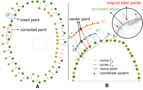
The processing object of our LLPC is a set of label points ($\left\{x_{s}^{i}\right\}$) corresponding to a closed contour. For an original label point $x_{s}^{i}$, we select candidate points along the normal direction of label edge, as shown in Figure 2A. These points constitute a candidate point set $\Omega_{x_{s}^{i}}$, and $x_{max}^{i}$ is the point with the largest gradient in $\Omega_{x_{s}^{i}}$. We move $x_{s}^{i}$ to the position of $x_{max}^{i}$ to obtain the corrected label point $x_{c}^{i}$.

$$x_{c}^{i}=\left\{\begin{matrix}&x_{max}^{i}&if\,\Delta>0\\ &x_{s}^{i}&otherwise\end{matrix}\right.$$ (1)

where

$$\Delta=\left|max(\omega_{j}\cdot g(x_{s_{j}}^{i}))-min(\omega_{j}\cdot g(x_{s_{j}}^{i}))\right|-\lambda_{t}\cdot max(\omega_{j}).$$ (2)

$x_{s_{j}}^{i}$ is a candidate point in $\Omega_{x_{s}^{i}}$. We judge whether a point $x_{s}^{i}$ is in strong gradient regions through $\Delta$. If $\Delta>0$, the point will be corrected; otherwise, it will not be moved. In this way, when the radius ($r$) of $\Omega_{x_{s}^{i}}$ is larger, our method can correct larger annotation errors. However, this will increase the correction error of label points due to image noise and interference from adjacent edges. To balance the contradiction, the gradient value of the candidate point $g(x_{s_{j}}^{i})$ is weighted by $\omega_{j}$, which allows setting a larger radius to correct larger annotation errors. We compute the weight as

$$\omega_{j}=K(\left\|x_{s_{j}}^{i}-x_{s}^{i}\right\|_{2},h_{1}),$$ (3)

where

$$K(x,\,h)=\kappa(x/h)/h.$$ (4)

$K(x,h)$ is a weighted kernel function with bandwidth $h$. $\kappa(x)$ is a Gaussian function with zero mean and one variance. After point correction, $\left\{x_{s}^{i}\right\}\to\left\{x_{c}^{i}\right\}$.

3.2 Piecewise Curve Fitting

The edge generated directly from the point set $\left\{x_{c}^{i}\right\}$ is not smooth due to the errors in point correction process (see Section 5.4). To eliminate the errors, we fit multiple curve segments and stitch them together. In the annotation process of manually drawing cell contours, the annotators perform dense point annotations near large curvatures and sparse annotations near small curvatures to accurately and quickly outline cell contours. Since the existence of large intervals is not conducive to curve fitting, we perform linear point interpolation (PI) on these intervals before curve fitting.

Figure 3: Merge multiple curves ($C_{1}$ and $C_{2}$) into one curve($C_{c}$).

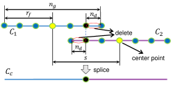
Point Interpolation. The sparse label point pairs can be represented as,

$$\left\{(x_{c}^{i},x_{c}^{i+1})|\left\|x_{c}^{i}-x_{c}^{i+1}\right\|_{2}>2\cdot gap\right\},$$ (5)

where $i=0,1\dots n_{s}-1$. Then, we insert points between the sparse points pairs to satisfy

$$\left\|x_{I}^{j}-x_{I}^{j+1}\right\|_{2}<gap,$$ (6)

as shown in Figure 2B. $j=0,1\dots n_{I}-1$. $n_{s}$ and $n_{I}$ are the number of points before and after interpolation, respectively. $gap$ is the maximum interval between adjacent point pair. After interpolation, $\left\{x_{c}^{i}\right\}\ \to\left\{x_{I}^{j}\right\}$.

Curve Fitting. We divide $\left\{x_{I}^{j}\right\}$ into $n_{c}$ groups. Each group is expressed as $\Phi_{k}=\left\{x_{I}^{1+k\cdot s},x_{I}^{2+k\cdot s},\dots,x_{I}^{n_{g}+k\cdot s}\right\}$. $k=0,1\dots n_{c}-1$. $n_{c}=\left\lceil n_{I}/s\right\rceil.$ As shown in Figure 3, $s=2(r_{f}-n_{d})$ is the interval between the center points of each group; $r_{f}=\left\lfloor(n_{g}-1)/2\right\rfloor$ is the group radius; $n_{g}$ is the number of points in the group. To reduce the fitting error at both ends of the curve, there is overlap between adjacent curves. The overlapping length is $2n_{d}$. To fit a curve on $\Phi_{k}$, we create a new coordinate system, as shown in Figure 2C. The x-axis passes through the $x_{I}^{1+k\cdot s}$ point and the $x_{I}^{n_{g}+k\cdot s}$ point. The point set in the new coordinate system is $\Phi_{k}^{r}$. We obtain a curve $C_{k}$ by local linear fitting [48] on $\Phi_{k}^{r}$. This is equivalent to solving the following problem at the target point $x_{t}=(x,y)$ on the curve $C_{k}$.

$$\underset{\beta_{0}(x),\,\beta_{1}(x)}{min}\sum_{j=1+k\cdot s}^{n_{g}+k\cdot s}\omega_{j}(x)(y_{j}-\beta_{0}(x)-\beta_{1}(x)\cdot x_{j})$$ (7)

$\beta_{0}(x)$ and $\beta_{1}(x)$ are the curve parameter at the point $x_{t}$. $(x_{j},y_{j})$ denotes the coordinates of point $x_{I}^{j}$ in $\Phi_{k}^{r}$. The weight function is

$$\omega_{j}(x)=K(\left\|x-x_{j}\right\|_{2},h_{2})/\sum_{m=1+k\cdot s}^{n_{g}+k\cdot s}K(\left\|x-x_{m}\right\|_{2},h_{2}).$$ (8)

If the distance between the point $x_{I}^{j}$ and the target point $x_{t}$ is larger, the weight $\omega_{j}(x)$ will be smaller. The matrix representation of the above parameter solution is

$$\beta=(X^{T}\omega X)^{-1}X^{T}\omega Y,$$ (9)

where $X=\begin{bmatrix}1&x_{1+k\cdot s}\\ 1&x_{2+k\cdot s}\\ \vdots&\vdots\\ 1&x_{n_{g}+k\cdot s}\end{bmatrix}$, $Y=\begin{bmatrix}y_{1+k\cdot s}\\ y_{2+k\cdot s}\\ \vdots\\ y_{n_{g}+k\cdot s}\end{bmatrix}$, $\beta=\begin{bmatrix}\beta_{0}(x)\\ \beta_{1}(x)\end{bmatrix}$, $\omega=\begin{bmatrix}\omega_{1+k\cdot s}(x)&&&\\ &\omega_{2+k\cdot s}(x)&&\\ &&\ddots&\\ &&&\omega_{n_{g}+k\cdot s}(x)\end{bmatrix}$. The matrix $\omega$ is zero except for the diagonal. Each $\Phi_{k}^{r}$ corresponds to a curve $C_{k}$. We stitch $n_{c}$ curves into a closed curve $C_{c}$, as shown in Figure 2C and Figure 3. Then, we sample on the interval $\left[x_{I}^{1+k\cdot s+n_{d}},x_{I}^{n_{g}+k\cdot s-n_{d}}\right]$ as shown in Figure 2D. We convert the coordinates of these sampling points to the original image coordinate system. Finally, we can obtain a discrete edge $C_{d}$, as shown in Figure 2E, F.

Figure 4: Local point smoothing to generate smooth closed discrete edges. (A) Insert points; (B) Move the coordinate system and correct each point by curve fitting. All corrected points constitute a discrete edge.

3.3 Local Point Smoothing

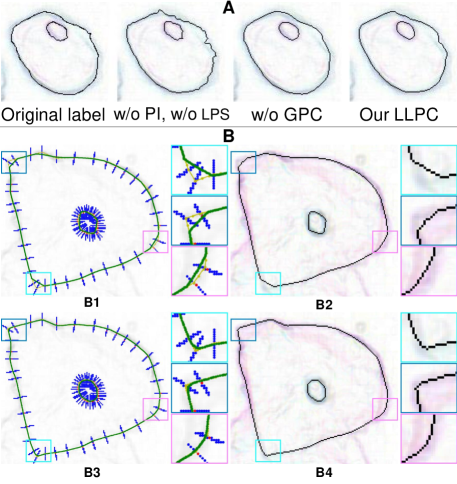
In Section 3.2, we stitch multi-segment curves to obtain a closed cell curve, and then sample the curve to generate a discrete edge. In fact, there is no smoothness at the splice nodes. To generate a smooth closed discrete edge, we design a local point smoothing (LPS) method without curves splicing and sampling. As shown in Figure 4A, we insert more points in large intervals ($gap=1$). As shown in Figure 4B, we only correct the center point of $\Phi_{k}^{r}$ by fitting a curve ($C_{k}$). By shifting the local coordinate system by one step ($s=1$), each point in $\left\{x_{I}^{j}\right\}$ will be corrected by fitting a curve. These correction points constitute a discrete edge $C_{d}$. Because no curves are spliced, the generated edge is smooth at each point. The pipeline of our LLPC is shown in Algorithm 1.

Input : $I$, a RGB image. $F$, a annotation file of $I$ ($F$ contains $k$ point lists). $r=15$, $\lambda_{t}=4$, $n_{g}=14$.

Output : The corrected discrete edge $C_{d}$.

1 $C_{d}$$\leftarrow$ [];

2 for $i\leftarrow 1$ to $k$ do

3       $x_{s}$$\leftarrow$ F[i];

4       $x_{c}$$\leftarrow$ GPC($x_{s},I,r,\lambda_{t}$) (based on Eq. 1);

5       $x_{I}$$\leftarrow$ PI($x_{c},gap=1$) (based on Eq. 6);

6       $x_{t}$$\leftarrow$ LPS($x_{I},n_{g}$) (based on Eq. 7);

7       $C_{d}$$\leftarrow$ Append ($C_{d},x_{t}$)

8 end for

Algorithm 1 LLPC Label Correction Algorithm.

3.4 Parameter Setting

In Section 3.1, we set the parameters $r=15$, $\lambda_{t}=4$ and $h_{1}=r/2$. In Section 3.2, we set $n_{g}=14$. $r_{f}=\left\lfloor(n_{g}-1)/2\right\rfloor$. $h_{2}=r_{f}/2$. When $gap=1$ and $s=1$, the Section 3.3 is a special case of the Section 3.2. See Section 5.4 for more discussion of parameter selection.

4 Experimental design

4.1 Data Aquisition and Processing

We compare our CCEDD with other cervical cytology datasets in Table 1. Our dataset was collected from Liaoning Cancer Hospital $\&$ Institute between 2016 and 2017. We capture digital images with a Nikon ELIPSE Ci slide scanner, SmartV350D lens and a 3-megapixel digital camera. For patients with negative and positive cervical cancer, the optical magnification is 100$\times$ and 400$\times$, respectively. All of the cases are anonymized. All processes of our research (image acquisition and processing, etc.) follow ethical principles. Our CCEDD dataset includes 686 cervical images with a size of 2048$\times$1536 pixels (Table 2). Six expert cytologists outline the closed contours of the cytoplasm and nucleus in cervical cytological images by an annotation software (labelme [49]).

Table 1: Comparison with other cervical cytology datasets. For a fair comparison of the sizes of different datasets, we crop the images to 512 $\times$ 512, and our CCEDD is about ten times larger than other datasets.

Dataset	Image size	Dataset size	Dataset size(512 $\times$ 512)	Open
ISBI [46]	1024 $\times$ 1024	17	68	$\surd$
SZU Dataset [47]	1360 $\times$ 1024	21	84	$\times$
BHU Dataset [11]	512 $\times$ 512	580	580	$\times$
CCEDD	2048 $\times$1536	686	8232	$\surd$

Table 2: The detailed description of CCEDD.

Our CCEDD	Uncut CCEDD	Cut CCEDD
Image size	2048 $\times$1536	512 $\times$ 384
Training set size	411	20139
Validation set size	68	3332
Test set size	207	10143
Dataset size	686	33614

Figure 5: Image cutting method. (A) 4$\times$4 cutting grid; (B) move the grid right; (C) move the grid down; (D) move the grid right and down.

We randomly shuffle our dataset and split it into training, validation and test sets. To ensure test reliability, we set this ratio to 6:1:3. To be able to train various complex neural networks on a GPU, we crop a large-size image into small-size images. If an image is cut as shown in Figure 5A, it will result in incomplete edge at the cut boundary. To maximize data utilization efficiency, we move the cutting grid, as shown in Figure 5B, C, D. After label correction, we cut an image with a size of 2048$\times$1536 into 49 image patches with a size of 512$\times$384 pixels.

4.2 Baseline Model and Evaluation Metrics

Baseline Model. Our baseline detectors are 10 state-of-the-art models. We evaluate multiple edge detectors, such as RCF [50], ENDE [51], DexiNed [52], FINED [53] and PiDiNet [54]. Furthermore, we explore more network structures for edge detection by introducing segmentation networks, which usually only requires simple modifications of the last layer of networks. These segmentation networks include STDC [55], UNet [56], UNet++ [57], CENet [58], MSU-Net [59]. To aggregate more shallow features for edge detection, we modify multiple layers of STDC, i.e., STDC+. More details of these network structure can be found in our code implementation.

Evaluation Metrics. We quantitatively evaluate the edge detection accuracy by calculating three standard measures (ODS, OIS and AP) [14]. The average precision (AP) is the area under the precision-recall curve (Figure 1B). F1-score$=\frac{2\cdot precision\cdot recall}{precision+recall}$ is the harmonic average of precision and recall. ODS is the best F1-score for a fixed scale, while OIS is the F1-score for the best scale in each image.

Figure 6: Visual comparison results on CCEDD dataset. (A) Slightly overlapping cells; (B)(C) Highly overlapping cells; (D)(E) Overlapping cell masses. (F)(G) Blurred overlapping cells; (H)(I) Overlapping cells in complex environments.

4.3 Experimental Setup

Training Strategy. Data augmentation can improve model generalization and performance [60]. In training, we perform rotation and shearing operations, which require padding zero pixels around an image. In testing, there is no zero pixel padding. This lead to different distributions of training and testing sets and degrade the model performance. Therefore, we perform data augmentation in pre-training and no augmentation during fine-tuning.

Due to the different structures and parameters of baseline networks, a fixed number of training iterations may lead to overfitting or underfitting. For accurate evaluation, we adaptively adjust the iteration number by evaluating the average accuracy (AP) on the validation set. The period of model evaluation is set 1 epoch for pre-training and 0.1 epoch for fine-tuning. After the $i$-th model evaluation, we can obtain $Model_{i}$ and $AP_{i}$ ($i=1,2,\cdots,50$). If $AP_{i}<min(AP_{i-j}$), the training ends and we obtain the optimal model $Model_{j|max(AP_{j})}$. $j=1,2,3$ in pre-training and $j=1,2,\cdots,10$ in fine-tuning. The maximum iteration number is 50 epochs for pre-training and fine-tuning. Besides, we also dynamically adjust the learning rate to improve performance. The learning rate $l$ decays from $1^{-4}$ to $1^{-5}$. If $AP_{i}<AP_{i-1}$, $l_{i}=l_{i-1}/2$.

Implementation Details. We use the Adam optimizer [61] to optimize all baseline networks on PyTorch ($\beta_{1}=0$, $\beta_{2}=0.9$). We use random normal initialization to initialize these networks. To be able to train various complex neural networks on a GPU, we resize the image to 256$\times$192. The batch size is set 4. We perform color adjustment, affine transformation and elastic deformation for data augmentation [60]. All experiments are implemented on a workstation equipped with a Intel Xeon Silver 4110 CPUs and a NVIDIA RTX 3090 GPU.

Table 3: Edge detection results on our CCEDD dataset. Our baseline model contains RCF [50], ENDE [51], DexiNed [52], FINED [53], PiDiNet [54], STDC [55], UNet [56], CE-Net [58], UNet++ [57], MSU-Net [59]. "BCELoss" is binary cross entropy loss function. "RCFLoss" is an annotator-robust loss function for edge detection [50]. STDC2 [55] has more parameters than STDC1 [55]. ”UNet++(DS)” is UNet++ [57] with deep supervision. ”MACs” is multiply–accumulate operation. ”Params” and ”MACs” are calculated by THOP. Best and second best results are highlighted and underlined.

Year/Model/Loss	$\Delta$AP($\%$)	Label correction			No label correction			Params(M)	MACs(G)
		AP	ODS	OIS	AP	ODS	OIS
2019/RCF/RCFLoss	41.0$\%$	0.612	0.599	0.594	0.434	0.485	0.485	14.81	19.56
2019/RCF/BCELoss	41.9$\%$	0.667	0.638	0.645	0.470	0.507	0.512
2019/ENDE/BCELoss	37.0$\%$	0.733	0.682	0.691	0.535	0.548	0.555	6.06	32.51
2020/DexiNed/RCFLoss	30.3$\%$	0.649	0.633	0.635	0.498	0.528	0.533	35.08	27.72
2020/DexiNed/BCELoss	38.5$\%$	0.723	0.671	0.680	0.522	0.541	0.549
2020/FINED/RCFLoss	28.4$\%$	0.602	0.604	0.450	0.469	0.510	0.402	1.43	14.38
2020/FINED/BCELoss	41.4$\%$	0.703	0.660	0.621	0.497	0.528	0.530
2021/PiDiNet/RCFLoss	37.2$\%$	0.590	0.581	0.574	0.430	0.481	0.479	0.69	3.74
2021/PiDiNet/BCELoss	42.7$\%$	0.648	0.624	0.628	0.454	0.496	0.501
2021/STDC1/BCELoss	12.9$\%$	0.394	0.466	0.472	0.349	0.438	0.443	14.26	4.48
2021/STDC1(pretrain)/BCELoss	13.1$\%$	0.407	0.478	0.483	0.360	0.451	0.454
2021/STDC2/BCELoss	16.1$\%$	0.403	0.473	0.478	0.347	0.435	0.442	22.30	7.01
2021/STDC2(pretrain)/BCELoss	15.0$\%$	0.413	0.484	0.488	0.359	0.449	0.454
2021/STDC1+/BCELoss	41.3$\%$	0.701	0.652	0.659	0.496	0.518	0.524	13.76	39.28
2021/STDC2+/BCELoss	38.2$\%$	0.694	0.648	0.656	0.502	0.525	0.532	21.83	41.81
2015/UNet/BCELoss	38.9$\%$	0.729	0.679	0.689	0.525	0.539	0.546	31.03	41.96
2019/CE-Net(pretrain)/BCELoss	37.5$\%$	0.696	0.653	0.658	0.506	0.530	0.535	60.24	17.36
2019/CE-Net/BCELoss	36.4$\%$	0.712	0.668	0.675	0.522	0.540	0.547
2019/UNet++(DS)/BCELoss	37.6$\%$	0.739	0.687	0.696	0.537	0.548	0.555	9.16	26.76
2019/UNet++/BCELoss	39.6$\%$	0.755	0.691	0.701	0.541	0.550	0.557		26.75
2021/MSU-Net/BCELoss	39.7$\%$	0.749	0.689	0.699	0.536	0.550	0.556	47.09	59.93

Figure 7: Visual comparison of different loss functions. (A) Input; (E) Ground Truth; (B)(F) PiDiNet [54]; (C)(G) RCF [50]; (D)(H) DexiNed [52]; (B)(C)(D) BCELoss; (F)(G)(H) RCFLoss [50]. "BCELoss" is binary cross entropy loss function. Compared with BCELoss, RCFLoss [50] can produce coarser edges.

5 Experimental Results and Discussion

5.1 Edge Detection of Overlapping Cervical Cells

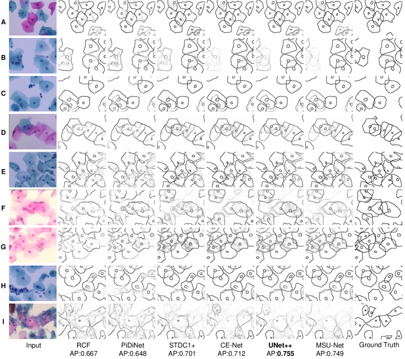
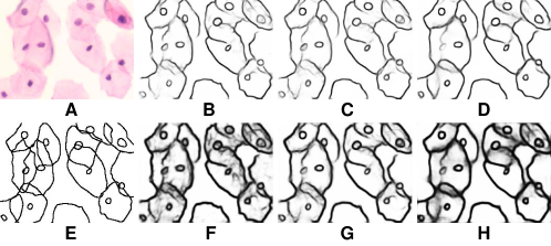
We show the visual comparison results on our CCEDD in Figure 6. The quantitative comparison is shown in Table 1 and Figure 1B. These results have important guiding implications for accurate edge detection of overlapping cervical cells. We analyze several factors affecting the performance of overlapping edge detection.

• Loss function design. RCFLoss [50] produces coarser edges, as shown in Figure 7. This may be robust for natural images, but poor localization accuracy for accurate cervical cell edge detection.

• Network structure design. Long-distance skip connections can fuse shallow and deep features for constructing multi-scale features. Our experiments show that the U-shaped structure is effective for overlapping edge detection (e.g., UNet [56], UNet++ [57] and MSU-Net [59]).

• Pre-training. Due to the huge distribution difference between natural and medical images, pre-training may degrade performance (e.g., CE-Net [58]) or have limited improvement (e.g., STDC [55]).

Figure 8: Label correction for edge detection and semantic segmentation. (A) Original edge; (B) Corrected edge; (C) Original mask; (D) Corrected mask.

Table 4: Performance improvement analysis of label correction. Use UNet++ [57] for evaluation.

Training / Evaluation	AP	ODS	OIS
Original label / Original label	0.541	0.550	0.557
Original label / Corrected label	0.588	0.592	0.598
Corrected label / Corrected label	0.755	0.691	0.701

5.2 Effectiveness of Label Correction

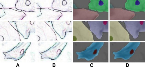
In our LLPC, the position of label points is locally corrected to the pixel gradient peak. As shown in Figure 1A and Figure 8B, Our LLPC can generate more accurate edge labels. Besides, we can easily generate corrected masks from corrected points in the labelme software [49]. Compared with the original mask in Figure 8C, our corrected mask has higher edge localization accuracy and smoother edges, as shown in Figure 8D.

Figure 9: Visual comparison results of training with different labels. (A) Input image; (B) UNet++ [57]/BCELoss + Original label; (C) UNet++ [57]/BCELoss + Corrected label; (D) Corrected labels. Compared with the original label, the corrected label can improve the accuracy of overlapping edge detection.

We train multiple networks using original label and corrected label. The quantitative comparison results is shown in Table 1 and Figure 1B. Compared with the original label, using the corrected label to train multiple networks can significantly improve AP (30-40$\%$), which verifies the effectiveness of our label correction method. Table 4 shows that the performance improvement comes from two aspects. First, our corrected label can improve the evaluation accuracy in testing (0.541$\to$0.588). Second, using our corrected label to train network can improve the accuracy of overlapping edge detection in training (0.588$\to$0.755), as shown in Figure 9.

Figure 10: Qualitative comparison of single-cell label correction. (A) Input; (B) Gradient image; (C) Original mask; (D) Input + original mask; (E) Active contours [62] for cytoplasm; (F) Active contours [62] for nucleus; (G) Dense CRF [45]; (H) Our LLPC.

5.3 Comparison with Other Label Correction Methods

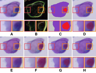
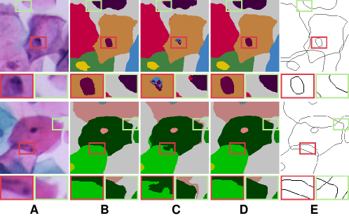
In Figure 10 and Figure 11, we compare our LLPC with active contours [62] and dense CRF [45]. We observed that active contours [62] is refinement failure of nucleus contours in Figure 10F, and dense CRF [45] fails due to complex overlapping cell contours in Figure 11C. Since active contours [62] and dense CRF [45] are global iterative optimization methods based on segmented images, which are uncontrollable for label correction of object contours and ultimately lead to these failed results. Our LLPC is the local label point correction without iterative optimization. Therefore, the correction error of our LLPC is controllable and the error in one place does not spread to other places, which is crucial for robust label correction. Besides, dense CRF [45] is nonplussed over overlapping instance segmentation refinement, while our LLPC corrects label based on annotation point and can handle overlapping label correction, as shown in Figure 11E.

Figure 11: Qualitative comparison of label correction for overlapping cell masses. (A) Input; (B) Original mask; (C) Dense CRF [45]; (D) Our LLPC (mask); (E) Our LLPC (edge).

Figure 12: (A) Ablation of gradient-guided point correction. "GPC" is gradient-guided point correction. (B) Visual comparison of different label correction methods. (B1) The green curves generated by piecewise curve fitting (w/o LPS); (B2) The discrete edge sampled from the curves in (B1); (B3) The curves smoothed by LPS; (B4) The discrete edges without curve sampling.

Table 5: Ablation of our LLPC. "GPC" is gradient-guided point correction. "PI" is point interpolation. "w/o LPS" is using piecewise curve fitting instead of local point smoothing. Use UNet++ [57] for evaluation.

Correction Method	AP	ODS	OIS
Original label	0.541	0.550	0.557
GPC (w/o PI, w/o LPS)	0.731	0.682	0.692
Our LLPC	0.755	0.691	0.701
w/o GPC	0.533	0.545	0.552
w/o PI	0.663	0.619	0.625
w/o LPS	0.742	0.689	0.699

5.4 Ablation experiment

Ablation of Label Correction Method. Our LLPC contains three steps: gradient-guided point correction (GPC), point interpolation (PI) and local point smoothing (LPS). Although our GPC can correct label points to pixel gradient peaks, there is still some error in the correction process. LPS can smooth the edges corrected by GPC, as shown in Figure 12A. Table 5 shows that GPC is the most important part of our LLPC (0.541$\to$0.731), while PI and LPS can further improve the annotation quality by smoothing edges (0.731$\to$0.755). Only smoothing the original labels ("w/o GPC") is ineffective (0.541$\to$0.533). Because this may lead to larger annotation errors. Compared to piecewise curve fitting in Section 3.2, LPS can generate smoother edges, as shown in Figure 12B. These qualitative and quantitative results verify that the three components of our LLPC are essential.

Table 6: Parameters ablation of our label correction method. Use UNet++ [57] for evaluation. For our CCEDD, we set $r=15,\lambda_{t}=4$ and $n_{g}=14$.

$r$	$\lambda_{t}$	$gap$	$n_{g}$	AP	ODS	OIS
7	4	1	14	0.691	0.645	0.653
11	4	1	14	0.732	0.681	0.691
19	4	1	14	0.746	0.691	0.701
23	4	1	14	0.734	0.683	0.692
15	1	1	14	0.750	0.689	0.700
15	2	1	14	0.751	0.690	0.700
15	3	1	14	0.745	0.691	0.700
15	5	1	14	0.750	0.689	0.699
15	10	1	14	0.729	0.679	0.688
15	15	1	14	0.708	0.658	0.664
15	4	1.5	14	0.749	0.688	0.698
15	4	2	14	0.742	0.689	0.699
15	4	1	10	0.750	0.689	0.699
15	4	1	12	0.729	0.687	0.697
15	4	1	16	0.752	0.690	0.700
15	4	1	18	0.750	0.687	0.698
15	4	1	14	0.755	0.691	0.701

Figure 13: Visual comparison results for different parameters settings in our LLPC. "default" is $r=15,\lambda_{t}=4$ and $n_{g}=14$. "w/o weight" is $\omega_{j}=1$ in Eq. 3.

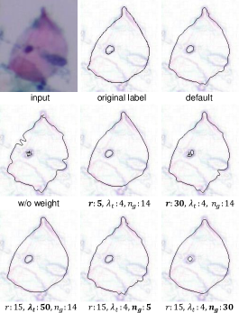
Selection of hyper-parameters. To set the optimal parameters, we conduct parameters ablation experiments in Table 6. $gap$ can control the point density in PI. For local curve fitting, $gap=1$ is optimal. Therefore, for an unknown dataset, our LLPC only needs to set three parameters, i.e., $r,\lambda_{t}$ and $n_{g}$. A qualitative comparison of these parameters with different settings is shown in Figure 13. $r$ controls the maximum error correction range in human annotations. If $r$ is too small, large label errors cannot be corrected. If $r$ is too large, the error of point correction is larger. $r$ limits the correction range in space, while $\lambda_{t}$ is the threshold for a limitation of gradient values variation during the correction process. If $\lambda_{t}$ is large, label points are corrected only when the gradient value changes sharply in the search direction. $n_{g}$ controls the scale of the local smoothing. For our CCEDD, $r=15,\lambda_{t}=4$ and $n_{g}=14$.

Table 7: Ablation of two-stage training strategy. We perform data augmentation in pre-training and no augmentation during fine-tuning. Use UNet++ [57] for evaluation.

Training methods	AP	ODS	OIS
w/o augmentation, w/o fine-tuning	0.729	0.672	0.683
w/ augmentation, w/o fine-tuning	0.732	0.674	0.682
w/ augmentation, w/ fine-tuning	0.755	0.691	0.701

Ablation of Training Strategy. Our training strategy can eliminate the influence of different distributions of the training and test sets due to data augmentation, and improve the AP by 3.6$\%$ in Table 7. To fairly evaluate multiple networks with different structures and parameters, we employ adaptive iteration and learning rate adjustment to avoid overfitting and underfitting. Table 8 and Figure 14A verify the effectiveness of our adaptive training strategy.

Table 8: Ablation of adaptive training strategy. We evaluate UNet++ [57] on the validation set. "AIT" is adaptive iteration training. "ALR" is adaptive learning rate.

Training methods	AP	ODS	OIS	epoch
w/o AIT, w/o ALR	0.683	0.639	0.642	50
w/o AIT, w/o ALR	0.449	0.653	0.657	70
w/o AIT, w/o ALR	0.308	0.647	0.653	100
w/ AIT, w/o ALR	0.747	0.684	0.693	13
w/ AIT, w/ ALR	0.750	0.693	0.700	21

Figure 14: (A) Training schedules. "AIT" is adaptive iteration training. "ALR" is adaptive learning rate. We evaluate UNet++ [57] on the validation set. (B) Comparison of network parameters, running efficiency and edge detection performance. ”MACs” is multiply–accumulate operation. "FPS" is the average speed by evaluating 10413 images with a resolution of 256$\times$192.

5.5 Computational Complexity

Label Correction. Our LLPC takes 270 seconds to generate 100 corrected edge images with a size of 2048$\times$1536 pixels on CPU. Because our label correction algorithm is offline and does not affect the inference time of a neural network, we have not further optimized it. If the algorithm runs on GPU, the speed can be further improved, which can save more time for label correction of large-scale datasets.

Model Evaluation. We rewrite the evaluation code [14] on GPU for fast evaluation. The average FPS using the UNet++ [57] is 173 for 10143 test images with a size of 256$\times$192 pixels. In training, we need to calculate the AP of the validation set to adaptively control the learning rate and the number of iterations (see Section 4.3). Fast evaluation greatly accelerates our training process.

Neural Network Inference. We test the inference speed of UNet++ [57]. For 207 images with a resolution of 1024$\times$768, the average FPS is 9. For 207 images with a resolution of 512$\times$512, the average FPS is 26. For 10413 images with a resolution of 256$\times$192, the average FPS is 295. Figure 14B shows the running efficiency comparison of multiple benchmark models. According to the report of Wan et al. [11], the methods of [11, 46, 63], took 17.67s, 35.69s and 213.62s for an image a resolution of 512$\times$512, respectively. Compared with these method, the UNet++ [57] is significantly faster. Many cervical cell segmentation approaches [11, 13, 64, 65, 66] consist of three stages, including nucleus candidate detection, cell localizations and cytoplasm segmentation. Fast edge detection of overlapping cervical cell means that the detected edges can be used as a priori input of these segmentation networks to improve performance at a small cost.

Figure 15: Label correction for natural images. (A) Original edge; (B) Corrected edge; (C) Original mask; (D) Corrected mask.

6 Discussion

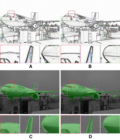
Label Correction for Natural Images. Our label correction method can correct a closed contour by correcting the position of label points, which does not require additional prior assumptions (e.g., contour shape, object size). We annotated several images in the PASCAL VOC dataset [67] with labelme [49] and corrected the label ($r=7,\lambda_{t}=4$ and $n_{g}=9$). As shown in Figure 15, our label correction method can generate more accurate object contours, which demonstrates the feasibility of our label correction method for natural images.

Overlapping Edge Detection. Overlapping edge detection of cervical cell is a challenging task due to the presence of strong and weak gradient edges. For edges with strong gradients, it only requires low-level detail features. For edges with weak gradients in overlapping region, it may require high-level semantics to reason contours and connect edges based on the context in strong gradient regions. While Unet++ [57] achieves the best results on our CCEDD, there is no difference in the detection of these two different types of edges. Designing new network structures and loss functions for overlapping edge detection may be a way to further address this challenge.

7 Conclusions

We propose a local label point correction method for edge detection and image segmentation, which is the first benchmark for label correction based on annotation points. Our LLPC can improve the edge localization accuracy and mitigate labeling error from different annotators in manual annotation. Only 3 parameters need to be set in our LLPC, but using the label corrected by our LLPC to train multiple networks can yield 30-40$\%$ AP improvement. Besides, we construct a largest overlapping cervical cell edge detection dataset based on our LLPC, which will greatly facilitate the development of overlapping cell edge detection. In future work, we plan to develop a label point correction method with local adaptive parameter adjustment.

Conflict of Interest Statement

The authors confirm that there are no conflicts of interest.

Author Contributions

JL: conceptualization, methodology, software, validation, writing - original draft, visualization. HF: investigation, resources, writing - review $\&$ editing, supervision, project administration, funding acquisition. QW: writing - review $\&$ editing. WL: investigation. YT: writing - review $\&$ editing, supervision. DW: investigation, resources, data curation. MZ and LC: investigation, resources. All authors contributed to the article and approved the submitted version.

FUNDING

This work is supported by the National Natural Science Foundation of China (61873259, 62073205, 61821005), the Key Research and Development Program of Liaoning (2018225037), and the Youth Innovation Promotion Association of Chinese Academy of Sciences (2019203).

Data Availability Statement

The datasets for this study can be found in https://github.com/nachifur/LLPC.

References

- [1] D. Demner-Fushman, M. D. Kohli, M. B. Rosenman, S. E. Shooshan, L. Rodriguez, S. Antani, G. R. Thoma, and C. J. McDonald, “Preparing a collection of radiology examinations for distribution and retrieval,” Journal of the American Medical Informatics Association, vol. 23, no. 2, pp. 304–310, 2016.
- [2] A. Almazroa, S. Alodhayb, E. Osman, E. Ramadan, M. Hummadi, M. Dlaim, M. Alkatee, K. Raahemifar, and V. Lakshminarayanan, “Agreement among ophthalmologists in marking the optic disc and optic cup in fundus images,” International Ophthalmology, vol. 37, no. 3, pp. 701–717, 2017.
- [3] A. E. W. Johnson, T. J. Pollard, N. R. Greenbaum, M. P. Lungren, C.-y. Deng, Y. Peng, Z. Lu, R. G. Mark, S. J. Berkowitz, and S. Horng, “MIMIC-CXR-JPG, a large publicly available database of labeled chest radiographs,” arXiv preprint arXiv:1901.07042, 2019. [Online]. Available: http://arxiv.org/abs/1901.07042
- [4] C. Zhang, D. Liu, L. Wang, Y. Li, X. Chen, R. Luo, S. Che, H. Liang, Y. Li, S. Liu, D. Tu, G. Qi, P. Luo, and J. Luo, “DCCL: A Benchmark for Cervical Cytology Analysis,” in Lecture Notes in Computer Science (including subseries Lecture Notes in Artificial Intelligence and Lecture Notes in Bioinformatics), vol. 11861 LNCS, 2019, pp. 63–72.
- [5] J. Ma, Y. Zhang, S. Gu, C. Zhu, C. Ge, Y. Zhang, X. An, C. Wang, Q. Wang, X. Liu, S. Cao, Q. Zhang, S. Liu, Y. Wang, Y. Li, J. He, and X. Yang, “AbdomenCT-1K: Is Abdominal Organ Segmentation A Solved Problem,” IEEE Transactions on Pattern Analysis and Machine Intelligence, p. 1, 2021.
- [6] Z. Lin, D. Wei, M. D. Petkova, Y. Wu, Z. Ahmed, K. S. K, S. Zou, N. Wendt, J. Boulanger-Weill, X. Wang, N. Dhanyasi, I. Arganda-Carreras, F. Engert, J. Lichtman, and H. Pfister, “NucMM Dataset: 3D Neuronal Nuclei Instance Segmentation at Sub-Cubic Millimeter Scale,” in Lecture Notes in Computer Science (including subseries Lecture Notes in Artificial Intelligence and Lecture Notes in Bioinformatics), vol. 12901 LNCS, 2021, pp. 164–174.
- [7] D. Wei, K. Lee, H. Li, R. Lu, J. A. Bae, Z. Liu, L. Zhang, M. dos Santos, Z. Lin, T. Uram, X. Wang, I. Arganda-Carreras, B. Matejek, N. Kasthuri, J. Lichtman, and H. Pfister, “AxonEM Dataset: 3D Axon Instance Segmentation of Brain Cortical Regions,” in Lecture Notes in Computer Science (including subseries Lecture Notes in Artificial Intelligence and Lecture Notes in Bioinformatics), vol. 12901 LNCS, 2021, pp. 175–185.
- [8] C. G. Northcutt, A. Athalye, and J. Mueller, “Pervasive label errors in test sets destabilize machine learning benchmarks,” arXiv preprint arXiv:2103.14749, 2021.
- [9] R. Saha, M. Bajger, and G. Lee, “Srm superpixel merging framework for precise segmentation of cervical nucleus,” in Digital Image Computing: Techniques and Applications, 2019, pp. 1–8.
- [10] Y. Song, J. Qin, B. Lei, S. He, and K.-S. Choi, “Joint shape matching for overlapping cytoplasm segmentation in cervical smear images,” in IEEE 16th International Symposium on Biomedical Imaging, 2019, pp. 191–194.
- [11] T. Wan, S. Xu, C. Sang, Y. Jin, and Z. Qin, “Accurate segmentation of overlapping cells in cervical cytology with deep convolutional neural networks,” Neurocomputing, vol. 365, pp. 157–170, 2019.
- [12] Y. Song, L. Zhu, B. Lei, B. Sheng, Q. Dou, J. Qin, and K.-S. Choi, “Constrained multi-shape evolution for overlapping cytoplasm segmentation,” arXiv preprint arXiv:2004.03892, 2020.
- [13] H. Zhang, H. Zhu, and X. Ling, “Polar coordinate sampling-based segmentation of overlapping cervical cells using attention u-net and random walk,” Neurocomputing, vol. 383, pp. 212–223, 2020.
- [14] P. Arbeláez, M. Maire, C. Fowlkes, and J. Malik, “Contour detection and hierarchical image segmentation,” IEEE Transactions on Pattern Analysis and Machine Intelligence, vol. 33, no. 5, pp. 898–916, 2011.
- [15] G. Zheng, A. H. Awadallah, and S. Dumais, “Meta Label Correction for Noisy Label Learning,” in Proceedings of the 35th AAAI Conference on Artificial Intelligence, 2019. [Online]. Available: http://arxiv.org/abs/1911.03809
- [16] J. Li, R. Socher, and S. C. H. Hoi, “DivideMix: Learning with Noisy Labels as Semi-supervised Learning,” in In Proceedings of the 8th international conference on learning representations, 2020. [Online]. Available: http://arxiv.org/abs/2002.07394
- [17] S. Bhadra and M. Hein, “Correction of noisy labels via mutual consistency check,” Neurocomputing, vol. 160, pp. 34–52, 2015.
- [18] B. Nicholson, V. S. Sheng, and J. Zhang, “Label noise correction and application in crowdsourcing,” Expert Systems with Applications, vol. 66, pp. 149–162, 2016.
- [19] B. Nicholson, J. Zhang, V. S. Sheng, and Z. Wang, “Label noise correction methods,” in IEEE International Conference on Data Science and Advanced Analytics, 2015, pp. 1–9.
- [20] J. Kremer, F. Sha, and C. Igel, “Robust active label correction,” in International Conference on Artificial Intelligence and Statistics, 2018, pp. 308–316.
- [21] K. Guo, R. Cao, X. Kui, J. Ma, J. Kang, and T. Chi, “Lcc: towards efficient label completion and correction for supervised medical image learning in smart diagnosis,” Journal of Network and Computer Applications, vol. 133, pp. 51–59, 2019.
- [22] S. Liu, J. Niles-Weed, N. Razavian, and C. Fernandez-Granda, “Early-learning regularization prevents memorization of noisy labels,” in Advances in Neural Information Processing Systems, vol. 2020-December, 2020.
- [23] X. Wang, Y. Hua, E. Kodirov, D. A. Clifton, and N. M. Robertson, “Proselflc: Progressive self label correction for training robust deep neural networks,” in Proceedings of the IEEE/CVF Conference on Computer Vision and Pattern Recognition, 2021, pp. 752–761.
- [24] S. Y. Li, Y. Shi, S. J. Huang, and S. Chen, “Improving deep label noise learning with dual active label correction,” Machine Learning, vol. 111, no. 3, pp. 1103–1124, 2022.
- [25] X. Zhu, G. Liu, B. Su, and J. P. Nees, “Dynamic label correction for distant supervision relation extraction via semantic similarity,” in CCF International Conference on Natural Language Processing and Chinese Computing, 2019, pp. 16–27.
- [26] N. P. Jouppi, C. Young, N. Patil, D. Patterson, G. Agrawal, R. Bajwa, S. Bates, S. Bhatia, N. Boden, A. Borchers, R. Boyle, P. L. Cantin, C. Chao, C. Clark, J. Coriell, M. Daley, M. Dau, J. Dean, B. Gelb, T. V. Ghaemmaghami, R. Gottipati, W. Gulland, R. Hagmann, C. Richard Ho, D. Hogberg, J. Hu, R. Hundt, D. Hurt, J. Ibarz, A. Jaffey, A. Jaworski, A. Kaplan, H. Khaitan, D. Killebrew, A. Koch, N. Kumar, S. Lacy, J. Laudon, J. Law, D. Le, C. Leary, Z. Liu, K. Lucke, A. Lundin, G. MacKean, A. Maggiore, M. Mahony, K. Miller, R. Nagarajan, R. Narayanaswami, R. Ni, K. Nix, T. Norrie, M. Omernick, N. Penukonda, A. Phelps, J. Ross, M. Ross, A. Salek, E. Samadiani, C. Severn, G. Sizikov, M. Snelham, J. Souter, D. Steinberg, A. Swing, M. Tan, G. Thorson, B. Tian, H. Toma, E. Tuttle, V. Vasudevan, R. Walter, W. Wang, E. Wilcox, and D. H. Yoon, “In-datacenter performance analysis of a tensor processing unit,” in Proceedings - International Symposium on Computer Architecture, vol. Part F128643, 2017, pp. 1–12.
- [27] Jia Deng, Wei Dong, R. Socher, Li-Jia Li, Kai Li, and Li Fei-Fei, “ImageNet: A large-scale hierarchical image database,” in 2009 IEEE Conference on Computer Vision and Pattern Recognition, 2009, pp. 248–255.
- [28] B. Zhou, A. Lapedriza, A. Khosla, A. Oliva, and A. Torralba, “Places: A 10 Million Image Database for Scene Recognition,” IEEE Transactions on Pattern Analysis and Machine Intelligence, vol. 40, no. 6, pp. 1452–1464, 2018.
- [29] C. Sun, A. Shrivastava, S. Singh, and A. Gupta, “Revisiting Unreasonable Effectiveness of Data in Deep Learning Era,” in Proceedings of the IEEE International Conference on Computer Vision, vol. 2017-October, 2017, pp. 843–852.
- [30] I. S. Alec Radford, Jeffrey Wu, Rewon Child, David Luan, Dario Amodei, “Language Models are Unsupervised Multitask Learners,” OpenAI Blog, vol. 1, no. May, pp. 1–7, 2020. [Online]. Available: https://github.com/codelucas/newspaper
- [31] C. Raffel, N. Shazeer, A. Roberts, K. Lee, S. Narang, M. Matena, Y. Zhou, W. Li, and P. J. Liu, “Exploring the limits of transfer learning with a unified text-to-text transformer,” Journal of Machine Learning Research, vol. 21, no. 140, pp. 1–67, 2020.
- [32] T. B. Brown, B. Mann, N. Ryder, M. Subbiah, J. Kaplan, P. Dhariwal, A. Neelakantan, P. Shyam, G. Sastry, A. Askell, S. Agarwal, A. Herbert-Voss, G. Krueger, T. Henighan, R. Child, A. Ramesh, D. M. Ziegler, J. Wu, C. Winter, C. Hesse, M. Chen, E. Sigler, M. Litwin, S. Gray, B. Chess, J. Clark, C. Berner, S. McCandlish, A. Radford, I. Sutskever, and D. Amodei, “Language models are few-shot learners,” in Advances in Neural Information Processing Systems, vol. 2020-December, 2020.
- [33] X. Hu, C. W. Fu, L. Zhu, J. Qin, and P. A. Heng, “Direction-aware spatial context features for shadow detection and removal,” IEEE Transactions on Pattern Analysis and Machine Intelligence, vol. 42, no. 11, pp. 2795–2808, 2020.
- [34] Z. Huang, Y. Wei, X. Wang, H. Shi, W. Liu, and T. S. Huang, “AlignSeg: Feature-Aligned Segmentation Networks,” IEEE Transactions on Pattern Analysis and Machine Intelligence, vol. 44, no. 1, pp. 550–557, 2021.
- [35] J. Zhao, S. Yan, and J. Feng, “Towards Age-Invariant Face Recognition,” IEEE Transactions on Pattern Analysis and Machine Intelligence, vol. 44, no. 1, pp. 474–487, 2022.
- [36] A. Ng, D. Laird, and L. He, “Data-Centric AI Competition,” https://https-deeplearning-ai.github.io/data-centric-comp/, 2021.
- [37] M. Motamedi, N. Sakharnykh, and T. Kaldewey, “A Data-Centric Approach for Training Deep Neural Networks with Less Data,” arXiv preprint arXiv:2110.03613, 2021. [Online]. Available: http://arxiv.org/abs/2110.03613
- [38] C. Sutton and A. McCallum, “An introduction to conditional random fields,” Foundations and Trends in Machine Learning, vol. 4, no. 4, pp. 267–373, 2011.
- [39] L. C. Chen, G. Papandreou, I. Kokkinos, K. Murphy, and A. L. Yuille, “Semantic image segmentation with deep convolutional nets and fully connected CRFs,” 3rd International Conference on Learning Representations, ICLR 2015 - Conference Track Proceedings, vol. 40, no. 4, pp. 834–848, 2015.
- [40] G. Sun, W. Wang, J. Dai, and L. Van Gool, “Mining Cross-Image Semantics for Weakly Supervised Semantic Segmentation,” in Lecture Notes in Computer Science (including subseries Lecture Notes in Artificial Intelligence and Lecture Notes in Bioinformatics), vol. 12347 LNCS, 2020, pp. 347–365.
- [41] X. Lu, W. Wang, J. Shen, D. Crandall, and L. Van Gool, “Segmenting Objects from Relational Visual Data,” IEEE Transactions on Pattern Analysis and Machine Intelligence, p. 1, 2021.
- [42] D.-P. Fan, T. Li, Z. Lin, G.-P. Ji, D. Zhang, M.-M. Cheng, H. Fu, and J. Shen, “Re-thinking Co-Salient Object Detection,” IEEE Transactions on Pattern Analysis and Machine Intelligence, p. 1, 2021.
- [43] T. Ma, Q. Wang, H. Zhang, and W. Zuo, “Delving Deeper Into Pixel Prior for Box-Supervised Semantic Segmentation,” IEEE Transactions on Image Processing, vol. 31, pp. 1406–1417, 2022.
- [44] Z. Zhang, Q. Peng, S. Fu, W. Wang, Y. M. Cheung, Y. Zhao, S. Yu, and X. You, “A Componentwise Approach to Weakly Supervised Semantic Segmentation Using Dual-Feedback Network,” IEEE Transactions on Neural Networks and Learning Systems, pp. 1–14, 2022.
- [45] P. Krähenbühl and V. Koltun, “Efficient inference in fully connected crfs with Gaussian edge potentials,” Advances in Neural Information Processing Systems 24: 25th Annual Conference on Neural Information Processing Systems 2011, NIPS 2011, vol. 24, 2011.
- [46] Z. Lu, G. Carneiro, and A. P. Bradley, “An improved joint optimization of multiple level set functions for the segmentation of overlapping cervical cells,” IEEE Transactions on Image Processing, vol. 24, no. 4, pp. 1261–1272, 2015.
- [47] Y. Song, E. L. Tan, X. Jiang, J. Z. Cheng, D. Ni, S. Chen, B. Lei, and T. Wang, “Accurate cervical cell segmentation from overlapping clumps in pap smear images,” IEEE Transactions on Medical Imaging, vol. 36, no. 1, pp. 288–300, 2017.
- [48] J. McCrary, “Manipulation of the running variable in the regression discontinuity design: A density test,” Journal of Econometrics, vol. 142, no. 2, pp. 698–714, 2008.
- [49] W. Kentaro, “labelme: Image Polygonal Annotation with Python (polygon, rectangle, circle, line, point and image-level flag annotation).” 2016. [Online]. Available: https://github.com/wkentaro/labelme
- [50] Y. Liu, M. Cheng, X. Hu, J. Bian, L. Zhang, X. Bai, and J. Tang, “Richer convolutional features for edge detection,” IEEE Transactions on Pattern Analysis and Machine Intelligence, vol. 41, no. 8, pp. 1939–1946, 2019.
- [51] K. Nazeri, E. Ng, T. Joseph, F. Qureshi, and M. Ebrahimi, “Edgeconnect: Structure guided image inpainting using edge prediction,” in Proceedings of the IEEE/CVF International Conference on Computer Vision Workshop, 2019, pp. 3265–3274.
- [52] X. S. Poma, E. Riba, and A. Sappa, “Dense extreme inception network: Towards a robust cnn model for edge detection,” in Proceedings of the IEEE/CVF Winter Conference on Applications of Computer Vision, 2020, pp. 1923–1932.
- [53] J. K. Wibisono and H.-M. Hang, “Fined: Fast inference network for edge detection,” arXiv preprint arXiv:2012.08392, 2020.
- [54] Z. Su, W. Liu, Z. Yu, D. Hu, Q. Liao, Q. Tian, M. Pietikäinen, and L. Liu, “Pixel difference networks for efficient edge detection,” in Proceedings of the IEEE/CVF International Conference on Computer Vision, 2021, pp. 5117–5127.
- [55] M. Fan, S. Lai, J. Huang, X. Wei, Z. Chai, J. Luo, and X. Wei, “Rethinking BiSeNet For Real-time Semantic Segmentation,” in Proceedings of the IEEE Computer Society Conference on Computer Vision and Pattern Recognition, 2021, pp. 9711–9720.
- [56] W. Weng and X. Zhu, “INet: Convolutional Networks for Biomedical Image Segmentation,” in IEEE Access, vol. 9, 2021, pp. 16 591–16 603.
- [57] Z. Zhou, M. M. R. Siddiquee, N. Tajbakhsh, and J. Liang, “Unet++: Redesigning skip connections to exploit multiscale features in image segmentation,” IEEE transactions on medical imaging, vol. 39, no. 6, pp. 1856–1867, 2019.
- [58] Z. Gu, J. Cheng, H. Fu, K. Zhou, H. Hao, Y. Zhao, T. Zhang, S. Gao, and J. Liu, “CE-Net: Context Encoder Network for 2D Medical Image Segmentation,” IEEE Transactions on Medical Imaging, vol. 38, no. 10, pp. 2281–2292, 2019.
- [59] R. Su, D. Zhang, J. Liu, and C. Cheng, “MSU-Net: Multi-Scale U-Net for 2D Medical Image Segmentation,” Frontiers in Genetics, vol. 12, p. 140, 2021.
- [60] M. D. Bloice, P. M. Roth, and A. Holzinger, “Biomedical image augmentation using augmentor,” Bioinformatics, vol. 35, no. 21, pp. 4522–4524, 2019.
- [61] D. P. Kingma and J. Ba, “Adam: A method for stochastic optimization,” in Proceedings of the 3rd International Conference on Learning Representations, vol. 1412, 2015.
- [62] T. F. Chan and L. A. Vese, “Active contours without edges,” IEEE Transactions on Image Processing, vol. 10, no. 2, pp. 266–277, 2001.
- [63] Z. Lu, G. Carneiro, A. P. Bradley, D. Ushizima, M. S. Nosrati, A. G. Bianchi, C. M. Carneiro, and G. Hamarneh, “Evaluation of Three Algorithms for the Segmentation of Overlapping Cervical Cells,” IEEE Journal of Biomedical and Health Informatics, vol. 21, no. 2, pp. 441–450, 2017.
- [64] A. Tareef, Y. Song, W. Cai, H. Huang, H. Chang, Y. Wang, M. Fulham, D. Feng, and M. Chen, “Automatic segmentation of overlapping cervical smear cells based on local distinctive features and guided shape deformation,” Neurocomputing, vol. 221, pp. 94–107, 2017.
- [65] H. A. Phoulady, D. Goldgof, L. O. Hall, and P. R. Mouton, “A framework for nucleus and overlapping cytoplasm segmentation in cervical cytology extended depth of field and volume images,” Computerized Medical Imaging and Graphics, vol. 59, pp. 38–49, 2017.
- [66] A. Tareef, Y. Song, H. Huang, D. Feng, M. Chen, Y. Wang, and W. Cai, “Multi-pass fast watershed for accurate segmentation of overlapping cervical cells,” IEEE Transactions on Medical Imaging, vol. 37, no. 9, pp. 2044–2059, 2018.
- [67] M. Everingham, S. M. Eslami, L. Van Gool, C. K. Williams, J. Winn, and A. Zisserman, “The Pascal Visual Object Classes Challenge: A Retrospective,” International Journal of Computer Vision, vol. 111, no. 1, pp. 98–136, 2015.