Competition of spatially inhomogeneous states in antiferromagnetic Hubbard model

Abstract

In this work we study zero-temperature phases of the anisotropic Hubbard model on a three-dimensional cubic lattice in a weak coupling regime. It is known that, at half-filling, the ground state of this model is antiferromagnetic (commensurate spin-density wave). For non-zero doping, various types of spatially inhomogeneous phases, such as phase-separated states and the state with domain walls (“soliton lattice”), can emerge. Using the mean-field theory, we evaluate the free energies of these phases to determine which of them could become the true ground state in the limit of small doping. Our study demonstrates that the free energies of all discussed states are very close to each other. Smallness of these energy differences suggests that, for a real material, numerous factors, unaccounted by the model, may arbitrary shift the relative stability of the competing phases. This further implies that purely theoretical prediction of the true ground state in a particular many-fermion system is unreliable.

I Introduction

I.1 Motivation

Investigations of inhomogeneous electronic states of different types constitute an active research area of modern condensed matter physics Zheng et al. (2000); Tranquada et al. (1995); Bianconi et al. (1996); Li et al. (2019); Dho et al. (2003); Miao et al. (2020); Zhu et al. (2016); Iwaya et al. (2011); Sing et al. (2017); Laplace et al. (2012); Kokanova and Rozhkov (2019); Luo and Dagotto (2014); Bianconi et al. (2015); Sboychakov (2013); Rakhmanov et al. (2013); Igoshev et al. (2015); Sheehy and Radzihovsky (2007); Narayanan et al. (2014). In this work, we study inhomogeneous states arising in the weakly doped antiferromagnetic (AFM) insulator. This physical situation is of interest in the context of cuprates Kivelson et al. (2003), pnictides Park et al. (2009), as well as other antiferromagnetic systems Narayanan et al. (2014). (Some non-magnetic superconducting systems may demonstrate Sheehy and Radzihovsky (2007) similar instabilities as well.) For the doped AFM materials inhomogeneities of different types, such as “stripes” (domain walls), phase separation, and “checkerboard” state, are discussed (see, e.g., Refs. Gorbatsevich et al., 1992; Kivelson et al., 2003; Park et al., 2009; Igoshev et al., 2010; Laplace et al., 2012; Dolgirev and Fine, 2017; Aristova et al., 2019; Fine, 2011; Narayanan et al., 2014; Rakhmanov et al., 2020).

Theoretically, many-body states hosting these types of inhomogeneities are quite common, and can be studied with the help of standard approximations Buzdin and Tugushev (1983); Rakhmanov et al. (2013); Sboychakov (2013); Igoshev et al. (2010, 2015). Often, various inhomogeneous phases compete against each other to become the true ground state of a model Hamiltonian. The outcome of this competition is usually presented Buzdin and Tugushev (1983); Igoshev et al. (2010); Rakhmanov et al. (2013); Igoshev et al. (2015) as a phase diagram that depicts how various states, both homogeneous and inhomogeneous, replace each other upon parameters variations. Yet, when comparing the model phase diagram against experimental data, one unavoidably has to address the following question: to which extent the diagram calculated within a simplified theoretical framework with the help of approximate approaches is robust in the presence of various perturbations unaccounted by the model or distorted by the approximations?

I.2 Our results

Answering the question formulated in the previous paragraph, it is often implicitly assumed that, although some variability of the phase boundaries is indeed unavoidable, the qualitative features of the diagram survive the reality check. In our study, we examine the latter assumption and demonstrate that the perceived stability is not automatically guaranteed at all. Namely, it will be shown that theoretically estimated energies of competing inhomogeneous states may be very close to each other. Consequently, which of these phases becomes the true ground state in a real system may be ultimately decided by factors external to the theoretical model, such disorder, longer-range interaction, lattice effects, etc.

Specific details of our investigation are as follows. We adopt the Hubbard model on the anisotropic cubic lattice as a study case. This model is widely used in the theoretical literature to describe large variety of many-fermion systems. To avoid non-controllable approximations, we limit ourselves to the regime of weak interactions. Stable antiferromagnetism in a weak coupling model is possible if the Fermi surface demonstrates pronounced nesting. Indeed, it is known that in the presence of nesting electronic liquid becomes unstable, and an AFM phase appears at arbitrary weak interaction. For the Hubbard model, the Fermi surface demonstrates perfect nesting at half-filling (one electron per a lattice site) and vanishing longer-range hopping amplitudes.

In the regime of weak coupling, Hamiltonians with nesting Rice (1970); Rakhmanov et al. (2013); Rozhkov et al. (2017); Chuang et al. (2001); Kiesel et al. (2012); Gor’kov and Teitel’baum (2010); Šimkovic IV et al. (2016); Mosoyan et al. (2018); Rakhmanov et al. (2018); Nandkishore et al. (2012); Sboychakov et al. (2017); González and Stauber (2019); Sboychakov et al. (2018); Rakhmanov et al. (2017); Akzyanov et al. (2014); Sboychakov et al. (2013a, b); Rozhkov (2009a, b, 2003); Hirschfeld et al. (2011); Fernandes and Schmalian (2010); Grüner (1994); Khokhlov et al. (2020) allow for consistent mean-field treatment of the AFM order. For example, Rice Rice (1970) used such a model to study AFM state in Cr and its alloys. It was later noted that in this class of theories, the doped AFM state is unstable with respect to phase separation of the injected electrons Rakhmanov et al. (2013). When the possibility of inhomogeneous state formation was taken into account, two scenarios of phase separation were identified: (i) separation into the paramagnetic and commensurate AFM states and (ii) separation into commensurate and incommensurate AFM states. Besides these, (iii) a phase with domain walls (sometimes called Buzdin and Tugushev (1983) “soliton lattice”) is also discussed in the literature Schulz (1989); Buzdin and Tugushev (1983); Zaanen and Gunnarsson (1989).

In our work, we investigate the relative stability of inhomogeneous states (i-iii). To determine which of them is energetically favorable, it is necessary to compare the free energies $F$ of these states. The free energies are calculated with the help of the mean-field approximation. As we have mentioned above, for all three states, the values of $F$ are virtually identical, at least at small doping. This finding and its implications are the main focus of this paper.

Our presentation is organized as follows. In Sec. II we discuss the Hubbard model and the mean-field approach used in calculations. In Sec. III we present calculations for the phase-separated states. The application of the mean-field approximation to the state with domain walls is explained in Sec. IV. Section V is dedicated to the discussion of the results. Some auxiliary results are relegated to two Appendices.

II Mean-field approach to the Hubbard model

We consider antiferromagnetic state of anisotropic Hubbard model on a three-dimensional (3D) cubic lattice in the weak coupling regime. The Hamiltonian of the model equals to

$$H = \sum_{\langle ij\rangle\sigma}t_{ij}\left(c_{i\sigma}^{{\dagger}}c^{\phantom{{\dagger}}}_{j\sigma}+H.c.\right)-\mu\sum_{i\sigma}c_{i\sigma}^{{\dagger}}c^{\phantom{{\dagger}}}_{i\sigma}+$$ (1)

$$+U\sum_{i}\left(n_{i\uparrow}-\frac{1}{2}\right)\!\left(n_{i\downarrow}-\frac{1}{2}\right),$$

where $c_{i\sigma}^{{\dagger}}$ and $c^{\phantom{{\dagger}}}_{i\sigma}$ are the creation and annihilation operators for an electron with spin projection $\sigma=\uparrow,\,\downarrow$ located in the site $i$, local density operator is $n_{i\sigma}=c_{i\sigma}^{{\dagger}}c^{\phantom{{\dagger}}}_{i\sigma}$, notation $\langle ij\rangle$ implies that sites $i$ and $j$ are nearest neighbors, and $t_{ij}$ represents the hopping amplitude connecting sites $i$ and $j$. Many antiferromagnetic materials (pnictides, cuprates, organic Bechgaard salts) demonstrate pronounced anisotropy. To model this feature, we explicitly assume that $t_{ij}$ are different for different orientations of the $\langle ij\rangle$-bond: when the bond is parallel to the $\alpha$-axis ($\alpha=x,\,y,\,z$), the amplitude is $t_{ij}=t_{\alpha}$.

In the second term of Eq. (1), $\mu$ is the chemical potential. The last term in Eq. (1) describes on-site Coulomb repulsion of electrons with opposite spin projections, with the interaction constant $U>0$. The terms $1/2$ in parentheses are added in order to chemical potential $\mu$ would equal to zero at half-filling (one electron per site).

We consider the Hubbard model (1) near the half-filling. At half-filling, the ground state of the Hubbard model is known to be antiferromagnetic Baeriswyl et al. (2013). It is assumed that small doping modifies but does not destroy the antiferromagnetic ordering.

In the antiferromagnetic state, the averaged number of spin-up electrons on site $i$ is not equal to the averaged number of spin-down electrons on the same site: $\langle n_{i\uparrow}\rangle\neq\langle n_{i\downarrow}\rangle$. We define the position-dependent order parameter

$$\Delta_{i}=\frac{U}{2}\left(\langle n_{i\uparrow}\rangle-\langle n_{i\downarrow}\rangle\right).$$ (2)

For the antiferromagnetic states with domain walls, the sum $\langle n_{i\uparrow}\rangle+\langle n_{i\downarrow}\rangle$ is also position dependent. Thus, it is useful to introduce the local doping level

$$x_{i}=\langle n_{i\uparrow}\rangle+\langle n_{i\downarrow}\rangle-1\,.$$ (3)

We study antiferromagnetic states of the model (1) in the weak coupling regime, when $U<W$, where $W$ is the bandwidth, $W=4\sum_{\alpha}t_{\alpha}$. In this case, the mean-field approach is the appropriate method to study the model (1). The mean-field scheme is based on the following replacement

$$n_{i\uparrow}n_{i\downarrow}\to\langle n_{i\uparrow}\rangle\,n_{i\downarrow}+\langle n_{i\downarrow}\rangle\,n_{i\uparrow}-\langle n_{i\uparrow}\rangle\langle n_{i\downarrow}\rangle\,.$$ (4)

Applying this substitution rule to Hamiltonian (1), one obtains

$$H\!\! = \!\!H_{\text{kin}}+H_{\text{int}}^{\rm MF},$$ (5)

$$H_{\text{kin}}\!\! = \!\!\!\sum_{\langle ij\rangle\sigma}t_{ij}\left(c_{i\sigma}^{{\dagger}}c^{\phantom{{\dagger}}}_{j\sigma}+H.c.\right)-\sum_{i\sigma}\mu^{\prime}_{i}c_{i\sigma}^{{\dagger}}c^{\phantom{{\dagger}}}_{i\sigma},$$ (6)

$$H_{\text{int}}^{\rm MF}\!\! = \!\!\sum_{i}\!\left[\Delta_{i}(c_{i\downarrow}^{{\dagger}}c^{\phantom{{\dagger}}}_{i\downarrow}\!-\!c_{i\uparrow}^{{\dagger}}c^{\phantom{{\dagger}}}_{i\uparrow})-U\!\left(\frac{x_{i}(2+x_{i})}{4}-\frac{\Delta_{i}^{2}}{U^{2}}\!\right)\!\right]\!,$$

where $\mu^{\prime}_{i}=\mu-Ux_{i}/2$ is the effective (position-dependent) chemical potential, which accounts for both $\mu$ and “Hartree” contribution $Ux_{i}/2$. Parameters $x_{i}$ and $\Delta_{i}$ are to be found self-consistently.

III Phase separated states

At zero doping the system’s ground state is the homogeneous commensurate AFM. When electrons or holes are added, the homogeneous state may become unstable. In this section we will investigate two specific scenarious of this instability. The simplest one is the phase separation into commensurate AFM and paramagnetic phases. Required calculations are straightforward and can be carried out analytically. A more comprehensive approach is to take the incommensurate AFM state into account. Corresponding calculations require numerical tools, however, the energy estimate is improved. We will see that the phase separation into incommensurate and commensurate AFM phases is more energetically favorable than the commensurate AFM/paramagnet separation.

III.1 Commensurate antiferromagnetism

We start our exposition with the simplest scenario: we assume that the doped system remains homogeneous $x_{i}=x=const$, and the order parameter is commensurate:

$$\Delta_{i}=(-1)^{i_{x}+i_{y}+i_{z}}\Delta,$$ (8)

where $\Delta=const$, and integers $i_{x}$, $i_{y}$, and $i_{z}$ describe the position of the lattice site $i=(i_{x},\,i_{y},\,i_{z})$. The calculations presented below will prove that such a state is unstable.

Taking into account Eq. (8), we make use of the Fourier transform to derive

$$H = \!\sum_{\mathbf{k}\sigma}\left(\varepsilon_{\bf k}-\mu^{\prime}\right)c_{{\bf k}\sigma}^{{\dagger}}c^{\phantom{{\dagger}}}_{{\bf k}\sigma}+$$ (9)

$$+\!\sum_{\mathbf{k}}\Delta\left(c_{{\bf k}\uparrow}^{{\dagger}}c^{\phantom{{\dagger}}}_{{\bf k}+{\bf Q}_{0}\uparrow}-c_{{\bf k}\downarrow}^{{\dagger}}c^{\phantom{{\dagger}}}_{{\bf k}+{\bf Q}_{0}\downarrow}\right)-$$

$$-U{\cal N}\left(\frac{x(2+x)}{4}-\frac{\Delta^{2}}{U^{2}}\right),$$

where $\mu^{\prime}=\mu-Ux/2$, the number of sites in the lattice is denoted by ${\cal N}$, vector ${\bf k}=(k_{x},k_{y},k_{z})$ is the quasi-momentum, and

$$\varepsilon_{\bf k}=-2\left[t_{x}\cos(k_{x})+t_{y}\cos(k_{y})+t_{z}\cos(k_{z})\right]$$ (10)

is the kinetic energy. At half-filling ($x=0$, $\mu=\mu^{\prime}\equiv 0$) the model’s Fermi surface nests perfectly, with ${\bf Q}_{0}=(\pi,\,\pi,\,\pi)$ as the nesting vector. Indeed, at the half-filling the Fermi surface is defined by the equation

$$\varepsilon_{\bf k}=0,$$ (11)

which remains invariant under translation by ${\bf Q}_{0}$, as guaranteed by the relation

$$\varepsilon_{{\bf k}+{\bf Q}_{0}}=-\varepsilon_{\bf k}.$$ (12)

While nesting is insensitive to the hopping anisotropy, it is destroyed by both longer-range hopping and finite $\mu$, or, equivalently, finite doping. It is the destruction of nesting by extra carriers that ultimately destabilizes the homogeneous state postulated at the beginning of this subsection.

To proceed with the solution, we introduce the four-component vector $\psi^{{\dagger}}_{\mathbf{k}}=(c^{{\dagger}}_{\mathbf{k}\uparrow},\,c^{{\dagger}}_{\mathbf{k}+\mathbf{Q}_{0}\uparrow},\,c^{{\dagger}}_{\mathbf{k}\downarrow},\,c^{{\dagger}}_{\mathbf{k}+\mathbf{Q}_{0}\downarrow})$. In terms of this vector, the Hamiltonian (9) can be written as

$$H=\sum_{\mathbf{k}}\psi^{{\dagger}}_{\mathbf{k}}\hat{H}_{\mathbf{k}}\psi^{\phantom{{\dagger}}}_{\mathbf{k}}-U{\cal N}\left(\frac{x(2+x)}{4}-\frac{\Delta^{2}}{U^{2}}\right),$$ (13)

where $4\times 4$ matrix $\hat{H}_{\mathbf{k}}$ is

$$\hat{H}_{\bf k}\!=\!\begin{pmatrix}\varepsilon_{\bf k}-\mu^{\prime}&\Delta&0&0\\ \Delta&\varepsilon_{{\bf k}+{\bf Q}_{0}}-\mu^{\prime}&0&0\\ 0&0&\varepsilon_{\bf k}-\mu^{\prime}&-\Delta\\ 0&0&-\Delta&\varepsilon_{{\bf k}+{\bf Q}_{0}}-\mu^{\prime}\end{pmatrix}.$$ (14)

Using Eq. (12), we express the eigenenergies as

$$E_{\mathbf{k}}^{(1,2)}=-\mu^{\prime}\mp\sqrt{\varepsilon_{\bf k}^{2}+\Delta^{2}}\,.$$ (15)

At zero temperature, the grand potential per site is

$$\Omega=\sum_{s}\!\int\!\frac{d^{3}{\bf k}}{(2\pi)^{3}}E^{(s)}_{\mathbf{k}}\Theta(-E^{(s)}_{\mathbf{k}})-U\left(\frac{x(2+x)}{4}-\frac{\Delta^{2}}{U^{2}}\right)\!.$$ (16)

Minimizing $\Omega$ with respect to $\Delta$ we obtain the equation for the order parameter. In the weak coupling limit, it is possible to solve this equation analytically (details are presented in Appendix A). This gives the following equation relating the gap $\Delta$ and the chemical potential $\mu^{\prime}$:

$$|\mu^{\prime}|+\sqrt{\mu^{\prime 2}-\Delta^{2}}=\Delta_{0}\,,$$ (17)

where $\Delta_{0}$ is the gap at half-filling [see Eq. (54) in Appendix A]. Since a typical experiment is performed at fixed doping, not fixed chemical potential, it is necessary to express the order parameter and the chemical potential as functions of the doping level $x$. The doping $x$ is given by the following relation:

$$x=\sum_{s}\!\int\!\frac{d^{3}{\bf k}}{(2\pi)^{3}}\,\Theta(-E^{(s)}_{\mathbf{k}})-1\,.$$ (18)

Acting in the same manner as described in Appendix A, we obtain in the weak coupling limit

$$x=2\rho_{0}\operatorname{sign}(\mu^{\prime})\sqrt{\mu^{\prime 2}-\Delta^{2}}\,,$$ (19)

where $\rho_{0}=\rho(0)$ is the density of states at zero energy [Fermi level at half-filling, see Eq. (51) for definition of $\rho(E)$]. If we set $\Delta=0$ in Eq. (19), we recover a familiar expression

$$\mu=\frac{x}{2\rho_{0}},$$ (20)

which relates doping and chemical potential in the paramagnetic phase. In Eq. (20) the contribution $Ux/2$ to the effective potential is omitted. The effects due to this term are small in the weak coupling limit, as we will show below.

Using equations (17) and (19), and neglecting $Ux/2$ contribution to $\mu^{\prime}$, we further obtain Rice (1970); Gorbatsevich et al. (1992)

$$|\mu| = \Delta_{0}\left(1-\frac{|x|}{2\rho_{0}\Delta_{0}}\right),$$ (21)

$$\Delta = \Delta_{0}\sqrt{1-\frac{|x|}{\rho_{0}\Delta_{0}}}\,.$$ (22)

These two formulas describe homogeneous AFM state. We note that the chemical potential is the decreasing function of the doping

$$\frac{\partial\mu}{\partial x}=-\frac{1}{2\rho_{0}}<0\,.$$ (23)

It means that the compressibility is negative and homogeneous AFM state is unstable, as announced above. This is the first example of the phase separation. Observe that the small correction to $\partial\mu/\partial x$ due to the omitted $Ux/2$ contribution to $\mu^{\prime}$ cannot restore the stability of the homogeneous state as long as we consider the weak coupling limit.

The structure of inhomogeneous phase can be established with the help of Maxwell construction, see Fig. 1. It shows the chemical potential of the homogeneous commensurate AFM state [decreasing line, Eq. (21)] and paramagnetic state [increasing line, Eq. (20)] versus the doping level. The horizontal line in Fig. 1 should be drawn so that areas $S_{1}$ and $S_{2}$ are equal. This line represents the phase-separated state. In thermodynamic equilibrium (that is, neglecting metastabile states), the chemical potential of the this state is

$$\mu_{\rm cAF}=\frac{\Delta_{0}}{\sqrt{2}}\approx 0.707\Delta_{0},$$ (24)

where the subscript ‘cAF’ stands for ‘commensurate antiferromagnet’. The neglected $Ux/2$ term introduces small correction (of the order of $U\rho_{0}\Delta_{0}$) to the value of $\mu_{\rm cAF}$.

The physical meaning of $\mu_{\rm cAF}$ is the threshold value which must be exceeded by the chemical potential of an external reservoir for doping to commence. The electrons injected into the AFM parent state, however, do not spread over the whole lattice evenly. Instead, as the Maxwell construction implies, the inhomogeneous state is split into areas of the undoped AFM and paramagnetic areas (the latter accumulate all the doping).

Figure 1: The doping dependence of the chemical potential for the commensurate AFM and paramagnetic phases. Chemical potential $\mu$ and doping $x$ are normalized by $\Delta_{0}$ and $\rho_{0}\Delta_{0}$, correspondingly. From $x=0$ to $x=\rho_{0}\Delta_{0}/2$ the chemical potential in the commensurate AFM phase is shown as a straight (red) line, see Eq. (21). Since this line has negative derivative, the doped commensurate AFM state is unstable. For the paramagnetic phase, $\mu=\mu(x)$ is shown as a straight (black) line, see Eq. (20). To determine the chemical potential of the phase-separated state, we use Maxwell construction: the horizontal dashed line is drawn to guarantee the equality of the areas $S_{1}=S_{2}$. The chemical potential of the inhomogeneous state is $\Delta_{0}/\sqrt{2}$. As one can see from the Maxwell construction, the separation occurs into the undoped AFM and the paramagnetic phases.

The main goal of the study is to determine which of the inhomogeneous states is energetically favorable. At fixed doping, this can be decided by comparison of the free energies $F(x)=\Omega+\mu x$ of the competing phases. For evaluation of $F(x)$, the following expression is useful

$$F(x)=F(0)+\int\limits_{0}^{x}\mu(x)dx\,,$$ (25)

where $F(0)$ is the free energy of undoped AFM insulator. Since the chemical potential is doping-independent in the phase-separated state, we derive

$$F_{\rm cAF}(x)=F(0)+\mu_{\rm cAF}x\,.$$ (26)

This expression is valid for sufficiently low doping, as long as the system remains on the horizontal line in Fig. 1. In the following sections, $F_{\rm cAF}$ will be compared with the free energies of other inhomogeneous states.

III.2 Incommensurate antiferromagnetism

We have seen in the previous section that at half-filling perfect nesting is realized at ${\bf Q_{0}}=\left(\pi,\pi,\pi\right)$. For finite doping the perfect nesting is impossible, but the quality of nesting may be improved if we consider incommensurate AFM, whose nesting vector is

$${\bf Q}=\left(\pi,\,\pi,\,\pi\right)+{\bf q}={\bf Q}_{0}+{\bf q}\,.$$ (27)

In this expression, ${\bf q}$ is (small) incommensurability vector. Non-zero $|{\bf q}|$ means that antiferromagnetic order parameter takes the form

$$\Delta_{i}=\Delta(-1)^{i_{x}+i_{y}+i_{z}}e^{i{\bf q}{\bf{r}}_{i}},$$ (28)

where $\mathbf{r}_{i}=(i_{x},\,i_{y},\,i_{z})$. The interaction part of the mean-field Hamiltonian in $k$-space becomes

$$H_{\text{int}}^{\rm MF} = \!\sum_{\mathbf{k}}\Delta\left(c_{{\bf k}\uparrow}^{{\dagger}}c^{\phantom{{\dagger}}}_{{\bf k}+{\bf Q}\uparrow}-c_{{\bf k}\downarrow}^{{\dagger}}c^{\phantom{{\dagger}}}_{{\bf k}+{\bf Q}\downarrow}\right)-$$ (29)

$$-U{\cal N}\left(\frac{x(2+x)}{4}-\frac{\Delta^{2}}{U^{2}}\right),$$

Taking into account the equation $\varepsilon_{\bf k+Q}=-\varepsilon_{\bf k+q}$, we can write the equations for eigenenergies

$$E^{(1,2)}_{\mathbf{k}}=-\mu^{\prime}+\frac{\varepsilon_{\bf k}-\varepsilon_{\bf k+q}}{2}\mp\sqrt{\left(\frac{\varepsilon_{\bf k}+\varepsilon_{\bf k+q}}{2}\right)^{2}+\Delta^{2}}\,.$$ (30)

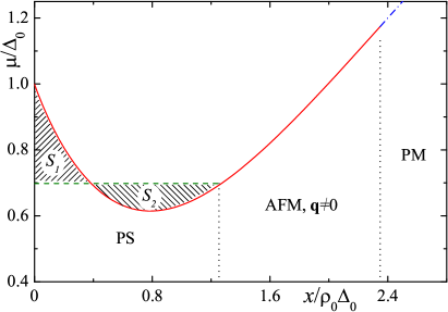
Figure 2: The doping dependence of the chemical potential of the incommensurate AFM state (solid red curve) and the paramagnetic state (blue dot-dashed curve). The Maxwell’s construction requires that the hatched areas $S_{1,2}$ are equal to each other. Horizontal dashed (green) line corresponds to the chemical potential of the phase-separated state. It equals to $\mu_{\rm iAF}/\Delta_{0}\cong 0.698$. Model parameters are $t_{x}=t_{y}=1$, $t_{z}=0.7$, incommensurability vector $\mathbf{q}$ is parallel to the $z$ axis.

Grand potential of the system per one site is given by Eq. (16) with eigenenergies from Eq. (30). The equations for the order parameter $\Delta$, nesting vector $\mathbf{q}$, and the chemical potential are

$$\frac{\partial\Omega}{\partial\Delta}=0\,,\;\;\frac{\partial\Omega}{\partial\mathbf{q}}=0\,,\;\;-\frac{\partial\Omega}{\partial\mu^{\prime}}=1+x\,.$$ (31)

These equations are soloved in the limit of small $|{\bf q}|$. The details of the calculations can be found in Refs. Rice, 1970; Rakhmanov et al., 2013; Sboychakov et al., 2013b (for reader’s convenience, they are outlined in Appendix B as well).

The resultant dependence $\mu=\mu(x)$ calculated for $\mathbf{q}$ parallel to the $z$ axis is plotted in Fig. 2 [hopping amplitudes corresponding to this figure are $(t_{x},\,t_{y},\,t_{z})=(1.0,\,1.0,\,0.7)$]. Here, as in the previous section, the small correction $Ux/2$ was neglected. We see non-monotonous behavior of $\mu(x)$, indicating the instability of the homogeneous state toward the phase separation, analogous to what Fig. 1 has shown. This time, however, the separated phases are (undoped) commensurate and incommensurate AFM states, as one can prove using the Maxwell construction. The chemical potential of the inhomogeneous state is

$$\mu_{\rm iAF}\approx 0.698\Delta_{0},$$ (32)

where the subscript ‘iAF’ stands for ‘incommensurate antiferromagnet’. When $\mathbf{q}$ is parallel to the $y$ axis, the dependence $\mu=\mu(x)$ is very similar to that shown in Fig. 2, except that the transition to the paramagnetic state in this case occurs at smaller doping.

Similar to $F_{\rm cAF}$, Eq. (26), the free energy $F_{\rm iAF}$ for the inhomogeneous phase represented by the horizontal line in Fig. 2 is

$$F_{\rm iAF}(x)=F(0)+\mu_{\rm iAF}x.$$ (33)

It is easy to see that

$$F_{\rm iAF}(x)<F_{\rm cAF}(x)\quad\Leftrightarrow\quad\mu_{\rm iAF}<\mu_{\rm cAF}.$$ (34)

Thus, the phase separation into the commensurate and incommensurate AFM phases is more favorable than the separation into the commensurate AFM state and the paramagnetic state.

It is interesting to note that Eq. (34) reduces the comparison of the free energies to the comparison of the threshold chemical potentials $\mu_{\rm cAF}$ and $\mu_{\rm iAF}$. Since these quantities are very close to each other ($\mu_{\rm iAF}\cong 0.698\Delta_{0}$ versus $\mu_{\rm cAF}\cong 0.707\Delta_{0}$), the energy difference between these two inhomogeneous states is very small for all relevant values of $x$.

IV A state with domain walls

IV.1 General considerations

Yet another type of inhomogeneous phase competing to become the true ground state is the phase with domain walls. In the previous section we have seen that, to decide which phase-separated state is more energetically favorable, the threshold chemical potentials have to be compared. In this section, we will calculate $\mu_{\rm dw}$, the threshold chemical potential for the phase with domain walls.

When the system’s chemical potential is close to the threshold value, the doping concentration is low (this is a direct consequence of the threshold chemical potential definition). A phase with domain walls in such a regime is characterized by large inter-wall separation and negligible interaction between the domain walls. Thus, $\mu_{\rm dw}$ is determined by the properties of a single domain wall.

Preparing a study of a single domain wall properties, several considerations must be taken into account. An important characteristics of a domain wall is its orientation relative to lattice axes. The vector normal to the domain wall plane may be parallel to one of the crystallographic axes, or it may point in an arbitrary direction Kato et al. (1990). All these orientations cannot be investigated in complete generality, and the study scope must be restricted. Numerical calculations for the arbitrary orientations of the domain walls are computationally costly. We expect that, in agreement with previous publications Zheng et al. (2017), the domain walls whose normal vectors are parallel to one of the axis are the most stable.

We study two types of domain walls: bond-centered and site-centered. They can be schematically depicted with the help of the following one-dimensional cartoons

$$\uparrow\downarrow\uparrow{\downarrow\downarrow}\uparrow\downarrow\uparrow\quad\text{bond-centered domain wall},$$

$$\uparrow\downarrow\uparrow{\downarrow{\rm o}\uparrow}\downarrow\uparrow\quad\text{site-centered domain wall}.$$

The arrows here represent the direction of the on-site spin magnetization, the symbol ‘o’ corresponds to a site with vanishing magnetization. As the name implies, in the middle of the bond-centered wall, there is a bond connecting two sites with identical magnetizations. A site with no net magnetization is in the middle of the site-centered wall. Despite obvious differences in real-space structures, our numerical simulations show that the energies of bond-centered and site-centered configurations are very close to each other.

IV.2 Mean-field description of a domain wall

Let us now outline the mean-field formalism we employ to study a single domain wall. For definiteness, we assume the domain wall is perpendicular to the $x$-axis. For such an orientation, the translation invariance in $y$ and $z$ directions is preserved, while it is explicitly broken in $x$-direction: the density of electrons and the order parameter are

$$\langle n_{i\uparrow}\rangle+\langle n_{i\downarrow}\rangle=n_{i_{x}},\,$$

$$\Delta_{i}=\Delta_{i_{x}}(-1)^{i_{y}+i_{z}}\,.$$ (35)

Therefore, it is convenient to switch to the mixed representation: in the $x$-direction, we continue using real space co-ordinate $i_{x}$, while in the transverse ($y$ and $z$) directions the 2D quasimomentum $\mathbf{p}=(p_{y},\,p_{z})$ is introduced. We also define the partial Fourier transform of $c^{{\dagger}}_{i\sigma}$ as follows

$$c^{{\dagger}}_{i_{x}\mathbf{p}\sigma}=\frac{1}{\sqrt{{\cal N}_{y}{\cal N}_{z}}}\sum_{i_{y},i_{z}}c^{{\dagger}}_{i\sigma}e^{i(p_{y}i_{y}+p_{z}i_{z})},$$ (36)

where ${\cal N}_{\alpha}$ is the number of unit cells along axis $\alpha=x,y,z$.

The mean-field Hamiltonian in the mixed representation reads

$$H = H_{\text{kin}}+H_{\text{int}}^{\rm MF}\,,$$ (37)

$$H_{\text{kin}} = \!\sum_{i_{x}\mathbf{p}\sigma}t_{x}\left(c^{{\dagger}}_{i_{x}\mathbf{p}\sigma}c^{\phantom{{\dagger}}}_{i_{x}+1\mathbf{p}\sigma}+H.c.\right)+$$ (38)

$$+\!\sum_{i_{x}\mathbf{p}\sigma}\left(\varepsilon^{\perp}_{\mathbf{p}}-\mu^{\prime}_{i_{x}}\right)c^{{\dagger}}_{i_{x}\mathbf{p}\sigma}c^{\phantom{{\dagger}}}_{i_{x}\mathbf{p}\sigma}\,,$$

$$H_{\text{int}}^{\rm MF} = -\!\sum_{i_{x}\mathbf{p}}\Delta_{i_{x}}\left(c^{{\dagger}}_{i_{x}\mathbf{p}\uparrow}c^{\phantom{{\dagger}}}_{i_{x}\mathbf{p}+\mathbf{P}_{0}\uparrow}-c^{{\dagger}}_{i_{x}\mathbf{p}\downarrow}c^{\phantom{{\dagger}}}_{i_{x}\mathbf{p}+\mathbf{P}_{0}\downarrow}\right)$$ (39)

$$-U\frac{\cal N}{{\cal N}_{x}}\sum_{i_{x}}\left(\frac{n_{i_{x}}^{2}-1}{4}-\frac{\Delta_{i_{x}}^{2}}{U^{2}}\right),$$

where $\mu^{\prime}_{i_{x}}=\mu-U(n_{i_{x}}-1)/2$. We also use the notations $\varepsilon^{\perp}_{\bf p}=-2t_{y}\cos(p_{y})-2t_{z}\cos(p_{z})$ and $\mathbf{P}_{0}=(\pi,\,\pi)$.

If we introduce the $2{\cal N}_{x}$-component vectors

$$\psi^{{\dagger}}_{\mathbf{p}\sigma}=\left(c^{{\dagger}}_{1\mathbf{p}\sigma}\,,\dots,\,c^{{\dagger}}_{{\cal N}_{x}\mathbf{p}\sigma}\,,c^{{\dagger}}_{1\mathbf{p}+\mathbf{P}_{0}\sigma}\,,\dots,\,c^{{\dagger}}_{{\cal N}_{x}\mathbf{p}+\mathbf{P}_{0}\sigma}\right)\!,\quad$$ (40)

the Hamiltonian (37) can be expressed as $H=\sum_{\mathbf{p}\sigma}\psi^{{\dagger}}_{\mathbf{p}\sigma}\hat{H}_{\mathbf{p}\sigma}\psi^{\phantom{{\dagger}}}_{\mathbf{p}\sigma}$, where the matrices $\hat{H}_{\mathbf{p}\sigma}$ can be written in the following block form

$$\hat{H}_{{\bf p}\uparrow}=\begin{pmatrix}\hat{H}_{0{\bf p}}&\hat{\Delta}\\ \hat{\Delta}&\hat{H}_{0{\bf p}+{\bf P}_{0}}\end{pmatrix},\;\hat{H}_{{\bf p}\downarrow}=\begin{pmatrix}\hat{H}_{0{\bf p}}&-\hat{\Delta}\\ -\hat{\Delta}&\hat{H}_{0{\bf p}+{\bf P}_{0}}\end{pmatrix}.$$ (41)

In the latter formulas, the matrices $\hat{H}_{0{\bf p}}$ and $\hat{\Delta}$ are

$$\hat{H}_{0{\bf p}}\! = \!\begin{pmatrix}\varepsilon^{\perp}_{\bf p}\!-\!\mu^{\prime}_{1}\!&t&0&\cdots&t\\ t&\varepsilon^{\perp}_{\bf p}\!-\!\mu^{\prime}_{2}\!&t&\cdots&0\\ 0&t&\varepsilon^{\perp}_{\bf p}\!-\!\mu^{\prime}_{3}\!&\cdots&0\\ \vdots&\vdots&\vdots&\ddots&\vdots\\ t&0&0&\cdots&\varepsilon^{\perp}_{\bf p}\!-\!\mu^{\prime}_{{\cal N}_{x}}\end{pmatrix}\!,\quad$$ (42)

$$\hat{\Delta}\! = \!\operatorname{diag}\left(\Delta_{1},\,...,\,\Delta_{{\cal N}_{x}}\right)\!.$$ (43)

Constructing the matrix $\hat{H}_{\mathbf{p}\sigma}$ we use periodic boundary conditions in the $x$-direction.

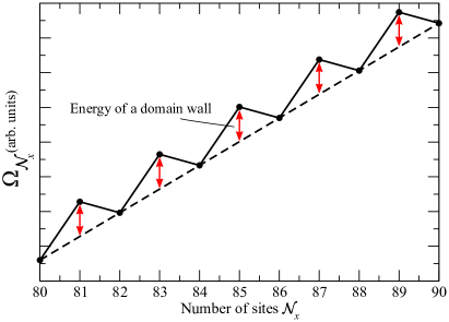
Figure 3: Schematic illustration of the dependence of the grand potential $\Omega_{{\mathcal{N}}_{x}}$ on the number of sites in the $x$-direction. For even ${\cal N}_{x}$, the dashed line represents proportionality $\Omega^{\rm even}_{{\cal N}_{x}}\propto{{\cal N}_{x}}$, see Eq. (45). When ${\cal N}_{x}$ is odd, $\Omega_{{\cal N}_{x}}$ is shifted by a constant value, see Eq. (46). This shift (shown by red arrows) is the energy of the domain wall $E_{\rm dw}$.

For the system with ${\cal N}_{x}$ unit cells along $x$-axis the grand potential $\Omega_{{\cal N}_{x}}$ (per unit area in $y$-$z$ plane) is

$$\Omega_{{\cal N}_{x}} = \sum_{\sigma}\sum_{S=1}^{{\cal N}_{x}}\int\frac{d^{2}{\bf p}}{(2\pi)^{2}}E^{(S)}_{{\bf p}\sigma}\Theta(-E^{(S)}_{{\bf p}\sigma})+$$ (44)

$$-U\sum_{i_{x}}\left(\frac{n_{i_{x}}^{2}-1}{4}-\frac{\Delta_{i_{x}}^{2}}{U^{2}}\right),$$

where $E^{(S)}_{{\bf p}\sigma}$ are the eigenenergies of the matrix $\hat{H}_{\mathbf{p}\sigma}$. To obtain $\Omega_{{\cal N}_{x}}$, the spatial dependencies of the order parameter $\Delta_{i_{x}}$ and the number of electrons per site $n_{i_{x}}$ minimizing $\Omega_{{\cal N}_{x}}$ are found using a numerical recurrent procedure.

Once $\Omega_{{\cal N}_{x}}$ is known, the energy of a single domain wall $E_{\rm dw}$ can be calculated. To find $E_{\rm dw}$, it is necessary to consider systems with even and odd values of ${\cal N}_{x}$ (this number must be much larger than the width of the domain wall). A system with even ${\cal N}_{x}$ is antiferromagnetically ordered and its grand potential (per unit area in $y-z$ plane) is directly proportional to ${\cal N}_{x}$

$$\Omega_{{\cal N}_{x}}^{\rm even}=\Omega_{0}{\cal N}_{x}\,,$$ (45)

where $\Omega_{0}$ is the grand potential per site of the system with homogeneous AFM ordering. A system with odd number of sites unavoidably contains a domain wall. Therefore, the grand potential (per unit area) for the systems with odd number of sites $\Omega_{{\cal N}_{x}}^{\rm odd}$ can be expressed as

$$\Omega_{{\cal N}_{x}}^{\rm odd}=\Omega_{0}{\cal N}_{x}+E_{\rm dw}\,,$$ (46)

where $E_{\rm dw}$ is the energy of the domain wall (per unit area in the transverse directions). The relations (45) and (46) are illustrated in Fig. 3. They allow us to extract $E_{\rm dw}$: analysing $\Omega^{\rm even}$ versus ${\cal N}_{x}$ dependence, we obtain $\Omega_{0}$, whose value is used to find $E_{\rm dw}$ from the data for $\Omega^{\rm odd}$.

IV.3 Numerical results

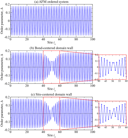
Figure 4: Spatial variation of the order parameter along $x$-axis, for even and odd values of ${\cal N}_{x}$. (a) When the number of sites in $x$-direction ${\cal N}_{x}$ is even, the antiferromagnetic order parameter maintains the same absolute value for all $i_{x}$, while the sign changes from one $i_{x}$ to the next. The data in the panel is plotted for ${\cal N}_{x}=100$. (b, c) When ${\cal N}_{x}$ is odd (specifically ${\cal N}_{x}=101$ for both panels), the antiferromagnetic domain wall emerges. Panel (b) shows the bond-centered domain wall. In the center of such a structure, we see two sites with identical values of the order parameters. The site-centered domain wall is in panel (c). This domain wall is centered on a site with vanishing order parameter. The simulations are performed for $U/W=0.17$, $(t_{x},\,t_{y},\,t_{z})=(1.0,\,1.0,\,0.7)$.

Numerically minimizing the grand potential $\Omega_{{\cal N}_{x}}$ we determine various properties of the studied system. Figure 4 demonstrates the spatial dependence of the order parameter for even and odd ${\cal N}_{x}$. As we can see from Fig. 4(a), the system with even number of sites has the homogeneous antiferromagnetic order: $\Delta_{i_{x}}$ has a constant absolute value and opposite signs on any pair of nearest sites. Naturally, the grand potential for such a state satisfies Eq. (45).

Due to the periodic boundary conditions, a system with odd number of sites cannot maintain unfrustrated antiferromagnetic order, and a domain wall appears. Because of the order parameter frustration, $\Delta_{i_{x}}$ is suppressed inside the domain wall, see Figs. 4(b,c). In our simulations, we can stabilize both bond-centered and site-centered domain walls. Figure 4(b) illustrates the order parameter structure for the bond-centered domain wall. Such a configuration possesses spatial reflection symmetry with respect to the center of the bond connecting the sites with minimum values of the order parameter. Site-centered domain wall is shown in Fig. 4(c). Spatial inversion relative to central site of the domain wall (the site with vanishing order parameter), accompanied by the spin flip $\mathbf{S}\to-\mathbf{S}$, preserves the site-centered configuration. Since bond-centered and site-centered domain walls have different symmetries, they represent mutually excluding classes of the mean-field solutions. Thus, they must be discussed separately. However, our simulations show that their energies are close to each other.

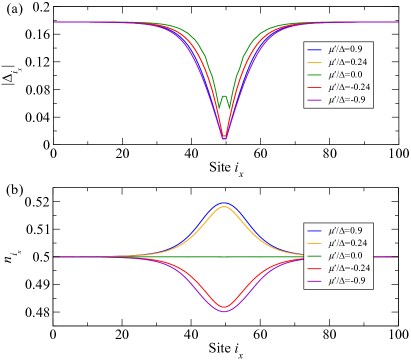
Figure 5: Spatial dependencies of (a) the absolute values of the order parameter $|\Delta_{i_{x}}|$, and (b) the electron density $n_{i_{x}}$, calculated for the bond-centered domain wall, at different values of the chemical potential $\mu^{\prime}$. Model parameters are: $U/W=0.17$, $(t_{x},\,t_{y},\,t_{z})=(1.0,\,1.0,\,0.7)$, and ${\cal N}_{x}=101$.

The domain wall properties are sensitive to the chemical potential. Indeed, Fig. 5 demonstrates the spatial dependencies of the absolute value of the order parameter and the electron density calculated for different values of $\mu^{\prime}=\mu-U(n-1)/2$ ($n$ is the averaged number of electrons per site) for the system with ${\cal N}_{x}=101$, $U/W=0.17$, and $(t_{x},\,t_{y},\,t_{z})=(1.0,\,1.0,\,0.7)$. One can see from this figure that even small deviation of the chemical potential from zero value sharply changes the order parameter and the electron density inside the domain wall. At higher values of $|\mu^{\prime}|$ the sensitivity of the order parameter and other quantities becomes less dramatic. Figure 5(a) shows that the order parameter is even function of $\mu^{\prime}$. Also, this figure demonstrates that the domain wall becomes wider when the chemical potential changes.

The accumulation of the injected charge carriers in the domain wall is illustrated by Fig. 5(b). At half-filling ($\mu^{\prime}=0$) there is one electron per site. When the chemical potential changes, the carriers pile up in the domain wall. For positive chemical potentials, the carriers are electrons, and for the negative ones, they are holes. Finally, Fig. 6 presents the domain wall energy and the total charge accumulated inside the domain walls (per unit area in $y$-$z$ plane) versus the chemical potential in the system with ${\cal N}_{x}=101$, $U/W=0.17$, and $(t_{x},\,t_{y},\,t_{z})=(1.0,\,1.0,\,0.7)$.

What can be understood from the numerical data about the properties of a single domain wall? We can see from Fig. 6 that the energy $E_{\rm dw}$ is the even function of the chemical potential. Similarly, Fig. 5(b) and Fig. 6(b) show that the accumulated charge is odd function of $\mu^{\prime}$. These features are consequences of the charge-conjugation symmetry of our model. This symmetry allows us to restrict our attention to positive value of the chemical potential.

On general grounds, one expects that at zero doping and zero chemical potential, the domain wall energy is positive, meaning that the state with the domain walls is energetically unfavorable. However, as the chemical potential grows, charges dope the domain walls, improving their stability. Figures 6(a,b) clearly illustrate these tendencies. Most importantly, there is a specific value of $\mu$ at which $E_{\rm dw}=0$. When $E_{\rm dw}$ vanishes, a state with no domain walls and a state with a domain wall are degenerate. The corresponding value of $\mu$ is the critical chemical potential $\mu_{\rm dw}$ for the state with domain walls: if $\mu>\mu_{\rm dw}$, the domain wall energy becomes negative, and domain walls carrying finite charge density enter the bulk of the system. As in the previous section,

$$F_{\rm dw}\approx F(0)+\mu_{\rm dw}x$$ (47)

at low $x$. This equation remains applicable as long as the distance between the domain walls is large, and the interaction between them may be neglected. As the concentration grows, the repulsion between the walls sets in, and Eq. (47) progressively becomes less accurate. In the regime of validity of Eqs. (26), (33), and (47) the competition between the inhomogeneous states is decided by the lowest critical chemical potential, as in Eq. (34).

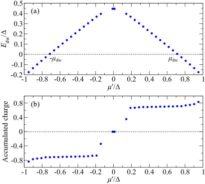
Figure 6: Chemical potential dependence of (a) the bond-centered domain wall energy $E_{\rm dw}$ and (b) the number of charge carriers in a domain wall. In panel (a) the critical chemical potential $\mu_{\rm dw}$ is marked. It corresponds to the value of $\mu$ at which the domain wall energy vanishes. Model parameters are: ${\cal N}_{x}=101$, $U/W=0.17$, and $(t_{x},\,t_{y},\,t_{z})=(1.0,\,1.0,\,0.7)$.

The critical potential calculated numerically is shown in Fig. 7 for three different anisotropies of “easy-plane” ($t_{x}=t_{y}>t_{z}$) type. We see that the critical chemical potential monotonically increases when the anisotropy increases. To perform consistent comparison of $\mu_{\rm dw}$ with $\mu_{\rm iAF}$ and $\mu_{\rm cAF}$, we need to find $\mu_{\rm dw}$ in the low-$U$ limit, as we did above to obtain the estimates (24) and (32). Numerical calculations at very low $U$ quickly become impossible since the width of the domain wall grows quickly as $U$ drops, and one has to increase the system size stretching computational resources. To circumvent this issue, $\mu_{\rm dw}$ at $U=0$ is evaluated extrapolating the available numerical data to zero value of $U$. The data points can be adequately fitted by linear functions, see Fig. 7. The resultant low-$U$ values of $\mu_{\rm dw}$ are shown in Fig. 8. Alternatively, the same data can be approximated by a quadratic function. This produces similar values of $\mu_{\rm dw}$, which are also plotted in Fig. 8.

The critical values of the chemical potential for different phases are ordered according to

$$\mu_{\rm dw}<\mu_{\rm iAF}\lesssim\mu_{\rm cAF}.$$ (48)

Thus, for the model under study, the state with the domain wall has the lowest energy, at least at low doping. As we announced from the very beginning, however, the energy difference separating the most stable phase and metastable “contenders” is insignificant. Indeed,

$$\mu_{\rm iAF}-\mu_{\rm dw}\lesssim 0.06\Delta_{0}$$ (49)

for all anisotropy parameters.

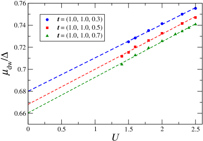
Figure 7: Critical chemical potential versus interaction constant $U$ for three different anisotropies (see legend). Linear fits are shown as dashed lines.

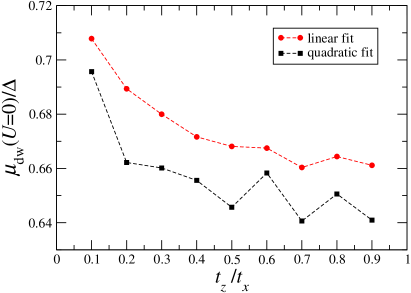
Figure 8: Critical chemical potential for the state with domain walls $\mu_{\rm dw}$ versus the hopping anisotropy parameter $t_{z}/t_{x}$, in the limit of low $U$, for the anisotropy of the “easy-plane” ($t_{x}=t_{y}>t_{z}$) type. The data points obtained by linear fit (quadratic function fit) are shown by red circles (black squares).

V Discussion and conclusions

In this paper we discuss inhomogeneous phases of the anisotropic Hubbard model. To avoid uncontrollable approximations, we limit ourselves to the weak coupling regime. Several interesting materials families, such as the Bechgaard salts and iron-based superconductors, are characterized by weak coupling. Electron-electron interaction in the cuprates superconductors is believed to be strong or intermediate, therefore, our results are not immediately applicable to the cuprates.

It is known that the homogeneous antiferromagnetic state of the Hubbard model at one electron per site loses its stability upon doping. This feature is not unique to the Hubbard Hamiltonian. Other models with nesting demonstrate similar instability. In the context of superconductivity, related phenomenon exists in the form of inhomogeneous Fulde-Ferrel-Larkin-Ovchinnikov states. Thus, destruction of the electronic liquid homogeneity is not limited to systems modelled by the Hubbard Hamiltonian with repulsion, but rather is of interest in many situations.

We discuss three specific inhomogeneous phases (two types of phase separated states and the state with domain walls) at zero temperature. It is argued that, at low doping, the free energies of these states can be characterized by a single parameter, critical chemical potential. The latter concept has simple physical meaning: if the chemical potential of a reservoir is lower than the critical chemical potential of a certain inhomogeneous state, doping of our system through formation of this state is impossible. It is clear from this definition that the phase with the lowest critical chemical potential is the most stable at low doping.

The critical chemical potentials for all three phases were evaluated within the mean field framework. Our calculations demonstrate that the state with the domain wall (so-called “soliton lattice”) is the most stable. However, all three values are close to each other, see Eq. (49). This feature implies that purely theoretical prediction of the inhomogeneous phase in the specific material is unreliable, as numerous material factors lie outside of simple theoretical models. We expect that the relative stability of various inhomogeneous states, competing to become the true ground state, is affected by the lattice effects, band structure details, Coulomb interaction screening, disorder pinning, and other features. Reliable description of the inhomogeneous states competition in specific materials appears to be impossible without experimental input. The use of phenomenological models might be helpful as well.

We already pointed out that our result is not directly applicable to the cuprate superconductors, since the interaction constant in these materials is not small. However, the theoretical issue addressed in this paper remains relevant for the cuprates as well: it is quite possible that several inhomogeneous states with almost identical energies compete against each other obfuscating the interpretation of experimental data.

To conclude, we studied inhomogeneous states of the Hubbard model in proximity to the half-filling. We demonstrated that the state with the domain walls is the most stable at low doping. However, the energies of metastable inhomogeneous states are found to be very close to the ground state energy. We argue that the smallness of this energy separation can introduce significant uncertainty into theoretical modeling of the inhomogeneous states of many-body systems.

Appendix A Details of the solution to the gap equation for the commensurate AFM state

At half-filling ($\mu^{\prime}=0$), minimization of the grand potential $\Omega$, Eq. (16), with respect to $\Delta$ gives the following equation

$$\frac{\partial\Omega}{\partial\Delta}=\Delta\left[\frac{2}{U}-\int\!\frac{d^{3}{\bf k}}{(2\pi)^{3}}\frac{1}{\sqrt{\Delta^{2}+\varepsilon_{\mathbf{k}}^{2}}}\right]=0\,.$$ (50)

Let us introduce the density of states

$$\rho(\varepsilon)=\int\!\frac{d^{3}{\bf k}}{(2\pi)^{3}}\,\delta(\varepsilon-\varepsilon_{\bf k})\,.$$ (51)

In the limit of small $\Delta\ll W$ studied here, we can rewrite the integral in the equation (50) in the form

$$\int\!\frac{d^{3}{\bf k}}{(2\pi)^{3}}\frac{1}{\sqrt{\Delta^{2}+\varepsilon_{\mathbf{k}}^{2}}}=\!\!\!\int\limits_{-W/2}^{W/2}\!\!\!d\varepsilon\,\frac{\rho(\varepsilon)}{\sqrt{\Delta^{2}+\varepsilon^{2}}}\cong$$

$$\cong\!\!\!\int\limits_{-W/2}^{W/2}\!\!\!d\varepsilon\,\frac{\rho(\varepsilon)-\rho_{0}}{|\varepsilon|}+\rho_{0}\!\!\!\int\limits_{-W/2}^{W/2}\!\!\!d\varepsilon\,\frac{1}{\sqrt{\Delta^{2}+\varepsilon^{2}}}\cong$$

$$\cong\frac{2}{U_{c}}+2\rho_{0}\ln\frac{W}{\Delta}\,,$$ (52)

where $\rho_{0}=\rho(0)$ is the density of states at the Fermi level, while parameter $U_{c}$ is defined by the equation

$$\frac{2}{U_{c}}=\!\!\!\int\limits_{-W/2}^{W/2}\!\!\!d\varepsilon\,\frac{\rho(\varepsilon)-\rho_{0}}{|\varepsilon|}\,.$$ (53)

Substituting Eq. (52) into Eq. (50), we obtain for the gap at half-filling:

$$\Delta_{0}=W\exp\left[-\frac{1}{\rho_{0}}\left(\frac{1}{U}-\frac{1}{U_{c}}\right)\right].$$ (54)

At finite doping, $\mu^{\prime}$ deviates from zero, and the equation for the order parameter can be expressed as (in the weak coupling limit)

$$2\ln\frac{\Delta_{0}}{\Delta}=\!\!\!\int\limits_{-W/2}^{W/2}\!\!\!d\varepsilon\,\frac{\Theta(|\mu^{\prime}|-\sqrt{\Delta^{2}+\varepsilon^{2}})}{\sqrt{\Delta^{2}+\varepsilon^{2}}}\,.$$ (55)

Evaluating the integral, one obtains Eq. (17) relating $\Delta$ and $\mu^{\prime}$.

Appendix B Details of the mean-field formalism for the incommensurate AFM state

In this Appendix, we will solve Eqs. (31). We start with the observation that in the limit of small $\Delta\ll W$, nesting vector ${\bf q}$ is also small: ${\bf q}\sim\Delta/W\ll 1$. In this regime, one can write

$$\varepsilon_{\bf k+q}\cong\varepsilon_{\bf k}+{\bf q}\frac{\partial\varepsilon_{\bf k}}{\partial\mathbf{k}}\,.$$ (56)

Calculating the derivatives of $\Omega$ with respect to $\Delta$, $\mathbf{q}$, and $\mu^{\prime}$, and using the smallness of $\Delta$ and $\mathbf{q}$ in a manner similar to that described in the Appendix A, we obtain the system of equations:

$$\ln\left(\frac{\Delta_{0}}{\Delta}\right)=\frac{1}{\rho_{0}}\!\!\int\limits_{-\eta_{0}}^{\eta_{0}}\!\!d\eta N(0,\eta)\operatorname{arccosh}{\left(\frac{|\mu^{\prime}-q\eta|}{\Delta}\right)},\quad$$ (57)

$$q\kappa=\!\!\int\limits_{\eta_{0}}^{\eta_{0}}\!\!d\eta N(0,\eta)\eta\sqrt{(\mu^{\prime}-q\eta)^{2}-\Delta^{2}}\operatorname{sign}(q\eta-\mu^{\prime}),\quad$$ (58)

$$x=2\!\!\int\limits_{\eta_{0}}^{\eta_{0}}\!\!d\eta N(0,\eta)\sqrt{(\mu^{\prime}-q\eta)^{2}-\Delta^{2}}\operatorname{sign}(\mu^{\prime}-q\eta),\quad$$ (59)

where we introduce the joint density of states

$$N(\xi,\eta)=\int\frac{d^{3}\mathbf{k}}{(2\pi)^{3}}\,\delta\left(\xi-\varepsilon_{\bf k}\right)\delta\left[\eta+{\hat{n}}_{\bf q}\frac{\partial\varepsilon_{\bf k}}{\partial\mathbf{k}}\right],$$ (60)

$$\eta_{0}=\max_{\bf k}{\left({\hat{n}}_{\bf q}\frac{\partial\varepsilon_{\bf k}}{\partial\mathbf{k}}\right)},\;\;\kappa=\!\!\int\limits_{-\eta_{0}}^{\eta_{0}}\!\!d\eta N(0,\eta)\eta^{2}\,,$$ (61)

and the unit vector ${\hat{n}}_{\bf q}={\bf q}/|{\bf q}|$ is collinear with $\mathbf{q}$.

Equations (57), (58), and (59) form a closed system of equations for self-consistent determination of $\Delta(x)$, $\mu(x)$, and $q(x)=|\mathbf{q}(x)|$ at the fixed direction of the nesting vector $\mathbf{q}$. We solve this system of equations for $(t_{x},\,t_{y},\,t_{z})=(1,\,1,\,0.7)$, and for two directions of $\mathbf{q}$: parallel to the $z$ axis and parallel to the $y$ axis. At relatively large doping, the state with $\mathbf{q}$ parallel to the $z$ axis is energetically more favorable, while at small doping the situation is opposite. However, the difference in free energies between these two cases turn out to be negligibly small. For the $z$ axis orientation, the data is shown in Fig. 2.

References

- Zheng et al. (2000) X. Zheng, C. Xu, Y. Tomokiyo, E. Tanaka, H. Yamada, and Y. Soejima, “Observation of charge stripes in cupric oxide,” Phys. Rev. Lett. 85, 5170 (2000).
- Tranquada et al. (1995) J. Tranquada, B. Sternlieb, J. Axe, Y. Nakamura, and S. Uchida, “Evidence for stripe correlations of spins and holes in copper oxide superconductors,” Nature 375, 561 (1995).
- Bianconi et al. (1996) A. Bianconi, N. Saini, A. Lanzara, M. Missori, T. Rossetti, H. Oyanagi, H. Yamaguchi, K. Oka, and T. Ito, “Determination of the Local Lattice Distortions in the CuO2 Plane of La1.85Sr0.15CuO4,” Phys. Rev. Lett. 76, 3412 (1996).
- Li et al. (2019) A. Li, J.-X. Yin, J. Wang, Z. Wu, J. Ma, A. S. Sefat, B. C. Sales, D. G. Mandrus, M. A. McGuire, R. Jin, et al., “Surface terminations and layer-resolved tunneling spectroscopy of the 122 iron pnictide superconductors,” Phys. Rev. B 99, 134520 (2019).
- Dho et al. (2003) J. Dho, Y. Kim, Y. Hwang, J. Kim, and N. Hur, “Strain-induced magnetic stripe domains in La0.7Sr0.3MnO3 thin films,” Appl. Phys. Lett. 82, 1434 (2003).
- Miao et al. (2020) T. Miao, L. Deng, W. Yang, J. Ni, C. Zheng, J. Etheridge, S. Wang, H. Liu, H. Lin, Y. Yu, et al., “Direct experimental evidence of physical origin of electronic phase separation in manganites,” PNAS 117, 7090 (2020).
- Zhu et al. (2016) Y. Zhu, K. Du, J. Niu, L. Lin, W. Wei, H. Liu, H. Lin, K. Zhang, T. Yang, Y. Kou, et al., “Chemical ordering suppresses large-scale electronic phase separation in doped manganites,” Nat. Commun. 7, 1 (2016).
- Iwaya et al. (2011) K. Iwaya, R. Shimizu, T. Ohsawa, T. Hashizume, and T. Hitosugi, “Stripe charge ordering in SrO-terminated SrTiO3 (001) surfaces,” Phys. Rev. B 83, 125117 (2011).
- Sing et al. (2017) M. Sing, H. O. Jeschke, F. Lechermann, R. Valentí, and R. Claessen, “Influence of oxygen vacancies on two-dimensional electron systems at SrTiO3-based interfaces and surfaces,” The European Physical Journal Special Topics 226, 2457 (2017).
- Laplace et al. (2012) Y. Laplace, J. Bobroff, V. Brouet, G. Collin, F. Rullier-Albenque, D. Colson, and A. Forget, “Nanoscale-textured superconductivity in Ru-substituted BaFe 2 As 2: A challenge to a universal phase diagram for the pnictides,” Phys. Rev. B 86, 020510 (2012).
- Kokanova and Rozhkov (2019) S. Kokanova and A. Rozhkov, “Disorder correction to the Néel temperature of ruthenium-doped BaFe2As2: Theoretical analysis,” Phys. Rev. B 99, 075134 (2019).
- Luo and Dagotto (2014) Q. Luo and E. Dagotto, “Magnetic phase diagram of a five-orbital Hubbard model in the real-space Hartree-Fock approximation varying the electronic density,” Phys. Rev. B 89, 045115 (2014).
- Bianconi et al. (2015) A. Bianconi, N. Poccia, A. O. Sboychakov, A. L. Rakhmanov, and K. I. Kugel, “Intrinsic arrested nanoscale phase separation near a topological Lifshitz transition in strongly correlated two-band metals,” Supercond. Sci. Technol. 28, 024005 (2015).
- Sboychakov (2013) A. Sboychakov, “Phase separation in strongly correlated electron systems with wide and narrow bands: A comparison of the Hubbard-I and DMFT approximations,” Physica B 417, 49 (2013).
- Rakhmanov et al. (2013) A. L. Rakhmanov, A. V. Rozhkov, A. O. Sboychakov, and F. Nori, “Phase separation of antiferromagnetic ground states in systems with imperfect nesting,” Phys. Rev. B 87, 075128 (2013).
- Igoshev et al. (2015) P. A. Igoshev, M. A. Timirgazin, V. F. Gilmutdinov, A. K. Arzhnikov, and V. Y. Irkhin, “Spiral magnetism in the single-band Hubbard model: the Hartree–Fock and slave-boson approaches,” J. Phys.: Condens. Matter 27, 446002 (2015).
- Sheehy and Radzihovsky (2007) D. E. Sheehy and L. Radzihovsky, “BEC-BCS crossover, phase transitions and phase separation in polarized resonantly-paired superfluids,” Annals of Physics 322, 1790 (2007).
- Narayanan et al. (2014) A. Narayanan, A. Kiswandhi, D. Graf, J. Brooks, and P. Chaikin, “Coexistence of Spin Density Waves and Superconductivity in (TMTSF)2PF6,” Phys. Rev. Lett. 112, 146402 (2014).
- Kivelson et al. (2003) S. A. Kivelson, I. P. Bindloss, E. Fradkin, V. Oganesyan, J. Tranquada, A. Kapitulnik, and C. Howald, “How to detect fluctuating stripes in the high-temperature superconductors,” Rev. Mod. Phys. 75, 1201 (2003).
- Park et al. (2009) J. T. Park, D. Inosov, C. Niedermayer, G. Sun, D. Haug, N. B. Christensen, R. Dinnebier, A. Boris, A. J. Drew, L. Schulz, et al., “Electronic phase separation in the slightly underdoped iron pnictide superconductor Ba1-xKxFe2As2,” Phys. Rev. Lett. 102, 117006 (2009).
- Gorbatsevich et al. (1992) A. Gorbatsevich, Y. Kopaev, and I. Tokatly, “Band theory of phase stratification,” Zh. Eksp. Teor. Fiz. 101, 971 (1992), [Sov. Phys. JETP 74, 521 (1992)].
- Igoshev et al. (2010) P. A. Igoshev, M. A. Timirgazin, A. A. Katanin, A. K. Arzhnikov, and V. Y. Irkhin, “Incommensurate magnetic order and phase separation in the two-dimensional Hubbard model with nearest- and next-nearest-neighbor hopping,” Phys. Rev. B 81, 094407 (2010).
- Dolgirev and Fine (2017) P. E. Dolgirev and B. V. Fine, “Pseudogap and Fermi surface in the presence of a spin-vortex checkerboard for 1/8-doped lanthanum cuprates,” Phys. Rev. B 96, 075137 (2017).
- Aristova et al. (2019) A. V. Aristova, V. K. Bhartiya, and B. V. Fine, “Modeling superconductivity in the background of a spin-vortex checkerboard,” Phys. Rev. B 100, 174503 (2019).
- Fine (2011) B. V. Fine, “Implications of Spin Vortex Scenario for 1/8-Doped Lanthanum Cuprates,” J. Supercond. Novel Magn. 24, 1207 (2011).
- Rakhmanov et al. (2020) A. L. Rakhmanov, K. I. Kugel, and A. O. Sboychakov, “Coexistence of Spin Density Wave and Metallic Phases Under Pressure,” Journal of Superconductivity and Novel Magnetism (2020).
- Buzdin and Tugushev (1983) A. Buzdin and V. Tugushev, “Phase diagrams of electronic and superconducting transitions to soliton lattice states,” Sov. Phys. JETP 58, 428 (1983).
- Rice (1970) T. M. Rice, “Band-Structure Effects in Itinerant Antiferromagnetism,” Phys. Rev. B 2, 3619 (1970).
- Rozhkov et al. (2017) A. V. Rozhkov, A. L. Rakhmanov, A. O. Sboychakov, K. I. Kugel, and F. Nori, “Spin-Valley Half-Metal as a Prospective Material for Spin Valleytronics,” Phys. Rev. Lett. 119, 107601 (2017).
- Chuang et al. (2001) Y.-D. Chuang, A. D. Gromko, D. S. Dessau, T. Kimura, and Y. Tokura, “Fermi Surface Nesting and Nanoscale Fluctuating Charge/Orbital Ordering in Colossal Magnetoresistive Oxides,” Science 292, 1509 (2001).
- Kiesel et al. (2012) M. L. Kiesel, C. Platt, W. Hanke, D. A. Abanin, and R. Thomale, “Competing many-body instabilities and unconventional superconductivity in graphene,” Phys. Rev. B 86, 020507 (2012).
- Gor’kov and Teitel’baum (2010) L. P. Gor’kov and G. B. Teitel’baum, “Spatial inhomogeneities in iron pnictide superconductors: The formation of charge stripes,” Phys. Rev. B 82, 020510 (2010).
- Šimkovic IV et al. (2016) F. Šimkovic IV, X.-W. Liu, Y. Deng, and E. Kozik, “Ground-state phase diagram of the repulsive fermionic Hubbard model on the square lattice from weak coupling,” Phys. Rev. B 94, 085106 (2016).
- Mosoyan et al. (2018) K. S. Mosoyan, A. V. Rozhkov, A. O. Sboychakov, and A. L. Rakhmanov, “Spin-density wave state in simple hexagonal graphite,” Phys. Rev. B 97, 075131 (2018).
- Rakhmanov et al. (2018) A. L. Rakhmanov, A. O. Sboychakov, K. I. Kugel, A. V. Rozhkov, and F. Nori, “Spin-valley half-metal in systems with Fermi surface nesting,” Phys. Rev. B 98, 155141 (2018).
- Nandkishore et al. (2012) R. Nandkishore, G.-W. Chern, and A. V. Chubukov, “Itinerant Half-Metal Spin-Density-Wave State on the Hexagonal Lattice,” Phys. Rev. Lett. 108, 227204 (2012).
- Sboychakov et al. (2017) A. O. Sboychakov, A. L. Rakhmanov, K. I. Kugel, A. V. Rozhkov, and F. Nori, “Magnetic field effects in electron systems with imperfect nesting,” Phys. Rev. B 95, 014203 (2017).
- González and Stauber (2019) J. González and T. Stauber, “Kohn-Luttinger Superconductivity in Twisted Bilayer Graphene,” Phys. Rev. Lett. 122, 026801 (2019).
- Sboychakov et al. (2018) A. O. Sboychakov, A. V. Rozhkov, A. L. Rakhmanov, and F. Nori, “Externally Controlled Magnetism and Band Gap in Twisted Bilayer Graphene,” Phys. Rev. Lett. 120, 266402 (2018).
- Rakhmanov et al. (2017) A. L. Rakhmanov, K. I. Kugel, M. Y. Kagan, A. V. Rozhkov, and A. O. Sboychakov, “Inhomogeneous electron states in the systems with imperfect nesting,” JETP Lett. 105, 806 (2017).
- Akzyanov et al. (2014) R. S. Akzyanov, A. O. Sboychakov, A. V. Rozhkov, A. L. Rakhmanov, and F. Nori, “AA-stacked bilayer graphene in an applied electric field: Tunable antiferromagnetism and coexisting exciton order parameter,” Phys. Rev. B 90, 155415 (2014).
- Sboychakov et al. (2013a) A. O. Sboychakov, A. L. Rakhmanov, A. V. Rozhkov, and F. Nori, “Metal-insulator transition and phase separation in doped AA-stacked graphene bilayer,” Phys. Rev. B 87, 121401 (2013a).
- Sboychakov et al. (2013b) A. O. Sboychakov, A. V. Rozhkov, K. I. Kugel, A. L. Rakhmanov, and F. Nori, “Electronic phase separation in iron pnictides,” Phys. Rev. B 88, 195142 (2013b).
- Rozhkov (2009a) A. V. Rozhkov, “Superconductivity without attraction in a quasi-one-dimensional metal,” Phys. Rev. B 79, 224520 (2009a).
- Rozhkov (2009b) A. V. Rozhkov, “Competition between different order parameters in a quasi-one-dimensional superconductor,” Phys. Rev. B 79, 224501 (2009b).
- Rozhkov (2003) A. V. Rozhkov, “Variational description of the dimensional crossover in an array of coupled one-dimensional conductors,” Phys. Rev. B 68, 115108 (2003).
- Hirschfeld et al. (2011) P. Hirschfeld, M. Korshunov, and I. Mazin, “Gap symmetry and structure of Fe-based superconductors,” Rep. Prog. Phys. 74, 124508 (2011).
- Fernandes and Schmalian (2010) R. M. Fernandes and J. Schmalian, “Competing order and nature of the pairing state in the iron pnictides,” Phys. Rev. B 82, 014521 (2010).
- Grüner (1994) G. Grüner, Density Waves In Solids (Addison-Wesley Publishing Company, 1994).
- Khokhlov et al. (2020) D. A. Khokhlov, A. L. Rakhmanov, A. V. Rozhkov, and A. O. Sboychakov, “Dynamical spin susceptibility of spin-valley half-metal,” (2020), arxive, eprint 2002.05504.
- Schulz (1989) H. Schulz, “Domain walls in a doped antiferromagnet,” J. Phys. France 50, 2833 (1989).
- Zaanen and Gunnarsson (1989) J. Zaanen and O. Gunnarsson, “Charged magnetic domain lines and the magnetism of high- oxides,” Phys. Rev. B 40, 7391 (1989).
- Baeriswyl et al. (2013) D. Baeriswyl, D. K. Campbell, J. M. Carmelo, F. Guinea, and E. Louis, The Hubbard model: its physics and mathematical physics, vol. 343 (Springer Science & Business Media, 2013).
- Kato et al. (1990) M. Kato, K. Machida, H. Nakanishi, and M. Fujita, “Soliton lattice modulation of incommensurate spin density wave in two dimensional hubbard model-a mean field study,” J. Phys. Soc. Jpn. 59, 1047 (1990).
- Zheng et al. (2017) B.-X. Zheng, C.-M. Chung, P. Corboz, G. Ehlers, M.-P. Qin, R. M. Noack, H. Shi, S. R. White, S. Zhang, and G. K.-L. Chan, “Stripe order in the underdoped region of the two-dimensional Hubbard model,” Science 358, 1155 (2017).