Small-Scale Dynamo in Supernova-Driven Interstellar Turbulence

Abstract

Magnetic fields grow quickly even at early cosmological times, suggesting the action of a small-scale dynamo (SSD) in the interstellar medium of galaxies. Many studies have focused on idealized turbulent driving of the SSD. Here we simulate more realistic supernova-driven turbulence to determine whether it can drive an SSD. Magnetic field growth occurring in our models appears inconsistent with simple tangling of magnetic fields, but consistent with SSD action, reproducing and confirming models by Balsara et al. (2004) that did not include physical resistivity $\eta$. We vary $\eta$, as well as the numerical resolution and supernova rate, $\dot{\sigma}$, to delineate the regime in which an SSD occurs. For a given $\dot{\sigma}$ we find convergence for SSD growth rate with resolution of a parsec. For $\dot{\sigma}\simeq\dot{\sigma}_{\rm sn}$, with $\dot{\sigma}_{\rm sn}$ the solar neighbourhood rate, the critical resistivity below which an SSD occurs is $0.005>\eta_{\rm crit}>0.001\,\rm kpc^{-1}\,\rm km~{}s^{-1}$, and this increases with the supernova rate. Across the modelled range of 0.5–4 pc resolution we find that for $\eta<\eta_{\rm crit}$, the SSD saturates at about 5% of kinetic energy equipartition, independent of growth rate. In the range $0.2\,\dot{\sigma}_{\rm sn}\leq\dot{\sigma}\leq 8\,\dot{\sigma}_{\rm sn}$ growth rate increases with $\dot{\sigma}$. SSDs in the supernova-driven interstellar medium commonly exhibit erratic growth.

1 Introduction

We here study the small-scale dynamo (SSD) in the interstellar medium (ISM). SSD acts at small eddy scales of turbulence, driving magnetic field growth at correspondingly short timescales. The large-scale dynamo (LSD) with much longer turnover times generates magnetic fields ordered on kiloparsec scales. Hence, capturing LSD alongside the faster growing modes of SSD in simulations is computationally challenging. However, interaction between SSD and LSD modes likely fundamentally determines the evolution and structure of the magnetic field.

Many simulations of supernova- (SN)-driven turbulence with realistic vertical stratification (e.g., de Avillez & Breitschwerdt, 2005; Piontek & Ostriker, 2007; Hill et al., 2012; Hennebelle & Iffrig, 2014) have no mechanism to induce LSD, such as rotation and shear. Strong ordered magnetic field effects are modelled by imposition of a background, typically uniform, magnetic field. Some large-scale models do seek to include LSD (e.g., Korpi et al., 1999; Gressel et al., 2008; Hanasz et al., 2009; Wang & Abel, 2009; Pakmor et al., 2017; Gressel & Elstner, 2020), but show no SSD, or appear to find SSD within the context of halo-disk scale flows (e.g., Rieder & Teyssier, 2016; Steinwandel et al., 2019), but capture no LSD. Gent et al. (2013a, with additional analysis by ) appear to include an SSD with an LSD. To confirm this and determine its effect on LSD, we must understand the properties of the SSD.

Any magnetic noise produced by tangling of a large-scale field will also grow exponentially if an LSD is present. This noise can play an important role in quenching the LSD. We need to discriminate this effect from an SSD.

Previous experiments (e.g., Balsara et al., 2004, hereafter BKMM4; Balsara & Kim, 2005; Mac Low et al., 2005) examined the SN-driven SSD. The limited resolution study of BKMM4 did not allow demonstration of solution convergence. Furthermore, they imposed a uniform background field and implemented no physical resistivity or viscosity. We shall show that the amplification of their field is a result of SSD action and not just tangling of the field.

In this Letter we first compare the SSD to tangling in an idealized simulation (Sect. 2). We then describe our models of SN-driven turbulence for demonstrating the action of SSD (Sect. 3). Simulations use the Pencil Code. A broad resolution and parameter study allows us to show numerical convergence and determine the critical resistivity for excitation of an SSD, which we follow to saturation (Sect. 4). This provides objective criteria for the action of SSD in simulations (such as Gent et al., 2013a; Gressel & Elstner, 2020; Steinwandel et al., 2019). Finally, we conclude in Sect. 5.

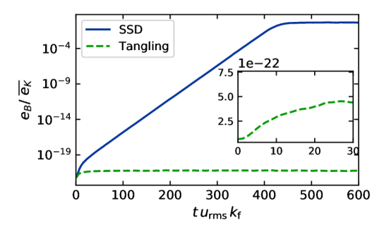
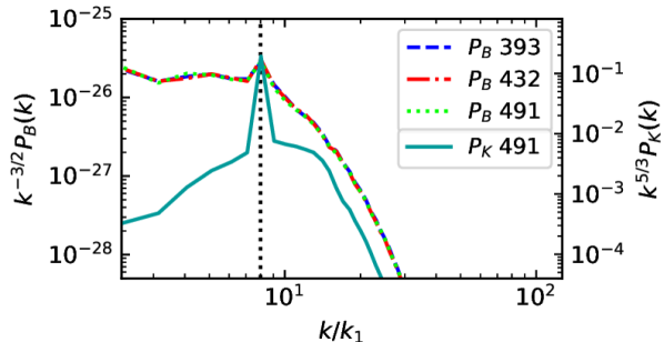
Figure 1: (a) Mean magnetic energy density, $e_{B}$, with nonhelical random forcing, scaled to time-averaged kinetic energy density, $\overline{e_{K}}$. Inset: early zoom-in of linear growth of tangled field. Time is normalised by eddy turnover time, $1/k_{\rm f}{u_{\rm rms}}$. Compensated power spectra of kinetic energy $P_{k}$ and magnetic energy $P_{B}$ for (b) SSD and (c) tangling, at times given in the legends. Kinetic energy uses the right-hand axes. Forcing scale, $k_{\rm f}/k_{1}=8$: vertical dotted line.

2 Disentangling the dynamo

Previous SSD studies have examined Pm dependence with stochastic nonhelical forcing, including at high Mach number (e.g., Haugen et al., 2003, 2004a, 2004b; Federrath et al., 2011, 2014). Here we specifically seek to illustrate differences between tangling and SSD. Nonhelical random forcing is applied at wavenumber $k_{\rm f}/k_{1}=8$ to $256^{3}$ zone, $2\pi$-periodic, isothermal boxes with viscosity $\nu=5\cdot 10^{-3}$. The lowest wavenumber in the domain is $k_{1}=1$ and the largest is the Nyquist frequency $k/k_{1}=128$. The imposed uniform field has $e_{B}\simeq 6\cdot 10^{-22}~{}\overline{e_{K}}$, where $\overline{e_{K}}$ is the time-averaged kinetic energy density.

Two simulations are distinguished by use of dimensionless resistivity $\eta=10^{-4}$ and $\eta=2\cdot 10^{-3}$. Respectively, these yield magnetic Reynolds number ${\rm Rm}=150$, with magnetic Prandtl number ${\rm Pm}=50$, exciting an SSD and ${\rm Rm}=7.4$, with ${\rm Pm}=2.5$, inhibiting the dynamo so that amplification is limited to tangling of the imposed field.

Figure 1 (a) shows the SSD growing exponentially in just over 400 eddy turnover times; see Zeldovich et al. (1983) for SSD properties and excitation conditions. Tangling induces only linear growth (see inset), saturating just above the imposed field energy within 50 turnover times.

Figures 1(b) and 1 (c) show compensated power spectra for both cases. Magnetic energy spectra are compensated for by Kazantsev’s $k^{3/2}$ power law (Schekochihin et al., 2002; Bhat & Subramanian, 2014), and kinetic energy by Kolmogorov’s $k^{-5/3}$. The forcing scale $k_{\rm f}$ is prominent in the magnetic energy spectra of the tangling but not in the magnetic spectra of the SSD. For SSD the range with Kazantsev power law (horizontal) extends to scales smaller than the forcing scale (Figure 1 b), and during the kinematic phase the magnetic energy peak is at $k/k_{1}\simeq 9$. For tangling (Figure 1 c) the Kazantsev scaling applies only at $k/k_{1}<k_{\rm f}$. Thus, in the SSD, kinetic energy in the Kolmogorov cascade transfers to magnetic energy at these scales, inducing an inverse Kazantsev cascade at scales smaller than $k_{\rm f}$, while tangling transfers energy only at scales between $k_{\rm f}$ and the scale of the imposed field.

3 Supernova-driven turbulence model design

Our SN-driven turbulence models exclude large-scale magnetic field dynamics by omitting global-scale rotation, shear, and stratification. Our simulation domain is a periodic cube of length 256 pc and zone size ${\delta x}=0.5$, 1, 2 or 4$~{}{\rm pc}$, except for our direct comparisons with BKMM4, which have domains of 200 pc and ${\delta x}=0.78$, 1.56 and 3.12$~{}{\rm pc}$ (units henceforth assumed). Our fiducial models exclude tangling of an imposed field as a source of magnetic amplification, by applying a random 10 nG initial field. Transient dissipation prior to hydrodynamic steady state and dynamo onset yields a turbulent seed field of about 1 nG. For models reproducing BKMM4 this seed is substituted by a uniform $10$ nG background field as applied by BKMM4.

Figure 2: 2D slices of (a, b) magnetic energy density $e_{B}$ and (c, d) gas density with shock dependent resistivity, $\zeta_{\eta}$, as indicated. The site of the most recent SN is indicated by X (c, d). ${\delta x}=1$ pc, $\eta=10^{-4}$ and $\nu=10^{-3}~{}{\rm km~{}s}^{-1}~{}{\rm kpc}^{-1}$.

We solve the system of non-ideal, compressible, non-isothermal MHD equations

$$\frac{D\rho}{Dt} = -\rho{{\mbox{\boldmath$\nabla$}}}\cdot{{\mbox{\boldmath$u$}}}+{{\mbox{\boldmath$\nabla$}}}\cdot\zeta_{D}{{\mbox{\boldmath$\nabla$}}}\rho,$$ (1)

$$\rho\frac{D{{\mbox{\boldmath$u$}}}}{Dt} = {{\mbox{\boldmath$\nabla$}}}{E_{\rm kin}\sigma}-\rho c_{\rm s}^{2}{{\mbox{\boldmath$\nabla$}}}\left({s}/{c_{\rm p}}+\ln\rho\right)+{{\mbox{\boldmath$j$}}}\times{{\mbox{\boldmath$B$}}}$$ (2)

$$+ {{\mbox{\boldmath$\nabla$}}}\cdot\left(2\rho\nu{\textbf{{W}}}\right)+\rho\,{{\mbox{\boldmath$\nabla$}}}\left(\zeta_{\nu}{{\mbox{\boldmath$\nabla$}}}\cdot{{\mbox{\boldmath$u$}}}\right)$$

$$+ {{\mbox{\boldmath$\nabla$}}}\cdot\left(2\rho\nu_{3}{\textbf{{W}}}^{(3)}\right){-{{\mbox{\boldmath$u$}}}{{\mbox{\boldmath$\nabla$}}}\cdot\left(\zeta_{D}{{\mbox{\boldmath$\nabla$}}}\rho\right)},$$

$$\rho T\frac{Ds}{Dt} = E_{\rm th}\dot{\sigma}+\rho\Gamma-\rho^{2}\Lambda+\eta\mu_{0}{{\mbox{\boldmath$j$}}}^{2}$$ (3)

$$+ 2\rho\nu\left|{\textbf{{W}}}\right|^{2}+\rho\,\zeta_{\nu}\left({{\mbox{\boldmath$\nabla$}}}\cdot{{\mbox{\boldmath$u$}}}\right)^{2}$$

$$+ {{\mbox{\boldmath$\nabla$}}}\cdot\left(\zeta_{\chi}\rho T{{\mbox{\boldmath$\nabla$}}}s\right)+\rho T\chi_{3}{{\mbox{\boldmath$\nabla$}}}^{6}s$$

$$- {c_{\rm{v}}\,T\left(\zeta_{D}\nabla^{2}\rho+{{\mbox{\boldmath$\nabla$}}}\zeta_{D}\cdot{{\mbox{\boldmath$\nabla$}}}\rho\right)},$$

$$\frac{\partial{{\mbox{\boldmath$A$}}}}{\partial t} = {{\mbox{\boldmath$u$}}}\times{{\mbox{\boldmath$B$}}}+\eta{{\mbox{\boldmath$\nabla$}}}^{2}{{\mbox{\boldmath$A$}}}+\eta_{3}{{\mbox{\boldmath$\nabla$}}}^{6}{{\mbox{\boldmath$A$}}},$$ (4)

with the ideal gas equation of state closing the system. Most variables take their usual meanings. Terms containing $\zeta_{D}{=2},\,\zeta_{\nu}=5$ and $\zeta{{}_{\chi}=2}$ are applied to all ISM models and resolve shock discontinuities with artificial diffusion of mass, momentum, and energy proportional to shock strength (see Gent et al., 2020, for details). Equations (2) and (3) include terms with $\zeta_{D}$ to provide momentum and energy conserving corrections for the artificial mass diffusion applying in Equation (1). In previous work Gent et al. (2013a) we have used a formalism that included artificial diffusion in vector potential at shocks. In Figure 2 we show comparative slices of the magnetic energy and gas density with and without resistive shock diffusion $\zeta_{\eta}$. With $\zeta_{\eta}>0$ (Fig. 2 b) magnetic energy is reduced in the remnant shell relative to Figure 2 a, where compression actually enhances it. Since the magnetic field is well resolved in either case, as also shown by the magnetic energy spectra below, and the simulation is numerically stable without it, this extra artificial diffusion is unnecessary.

In both models a concentration of magnetic energy, marked with $+$ in Figure 2, has below average gas density. This snapshot reflects the overall behaviour of the system, in which magnetic field amplification also occurs independently of shock compression. As Figure 2 shows, SN shock fronts do compress and amplify the magnetic field, resulting in strong local and instantaneous correlation of the field and density. However, on global and long-term scale, this is not the dominant mechanism for the dynamo, which operates just as effectively in the non-shocked, more diffuse regions, as is also indicated by this figure. This is based on the amplification factor due to compression being estimated $\lesssim 2$, taken as density fluctuations to power $4/3$, while the magnetic energy is amplified by 4–6 orders of magnitude.

Unlike past experiments (Gent et al., 2013a, b, 2020), thermal diffusivity $\chi$ is also omitted, as the artificial diffusivities chosen are adequate to ensure numerical stability. The physical effects of thermal conductivity can be expected to be relevant only at the unresolved or marginally resolved Field length defined by Begelman & McKee (1990, named after George Field, not the magnetic field). Terms containing $\nu_{3},\,\chi_{3}$ and $\eta_{3}$ apply sixth-order hyperdiffusion to resolve grid-scale instabilities (see, e.g., Brandenburg & Sarson, 2002; Haugen & Brandenburg, 2004), with mesh Reynolds number set to be $\simeq 1$ for each ${\delta x}$.

The simplified isothermal model considered in Sect. 2 solves only Equations (1), (2) and (4), without the shock-dependent diffusion or hyperdiffusion terms, and while setting ${{\mbox{\boldmath$B$}}}={{\mbox{\boldmath$\nabla$}}}\times{{\mbox{\boldmath$A$}}}+{{\mbox{\boldmath$B$}}}_{\rm imposed}$.

In the ISM simulations SNe are exploded at uniform random positions at a Poisson rate $\dot{\sigma}$ scaled by the solar neighborhood value $\dot{\sigma}_{\rm sn}\simeq 50~{}{\rm kpc}^{-3}~{}{\rm Myr}^{-1}$. Explosions inject $E_{\rm th}=10^{51}~{}{\rm erg}$ thermal energy, except in dense regions, where a proportion ($<5\%$) may be kinetic $E_{\rm kin}$ (see Gent et al., 2020). Models with common $\dot{\sigma}$ have the same timing and location of explosions. Non-adiabatic heating $\Gamma$ and cooling $\Lambda(T)$ are included (Gent et al., 2013a) following Wolfire et al. (1995) and Sarazin & White (1987).

Figure 3: Magnetic energy density shown for resolutions ${\delta x}$ given in the legends for models with resistivity (a) $\eta=10^{-4}$, and (b) $\eta=10^{-3}$, scaled by the time-averaged kinetic energy density $\overline{e_{K}}$. Total magnetic energy, $E_{B}$ scaled by $E_{\rm th}$, (c) matching BKMM4 for ${\delta x}$ and viscosity $\nu$ included in the legend and (d) kinetic energy, $E_{K}$, for ${\delta x}$, $\eta$ and $\dot{\sigma}$ given in the legend with corresponding magnetic energy (dotted).

To understand the effects of purely numerical diffusivity, we also run an ideal MHD model with $\eta=0$ and $\nu=0$. We determine how low a physical resistivity $\eta$ can be resolved by varying it from $10^{-5}$ to $10^{-3}~{}{\rm kpc}~{}{\rm km~{}s}^{-1}$ (units assumed henceforth). We also test the effect of ${\rm Pm}=\nu/\eta$, varying $\nu$ with $\eta=10^{-4}$ or varying $\eta$ with $\nu=10^{-3}$. Our direct comparison with the results of BKMM4 uses ${\rm Pm}=2.5$, apart from one run using $\eta=\nu=0$.

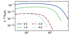
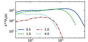
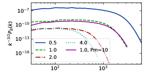
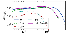
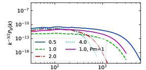
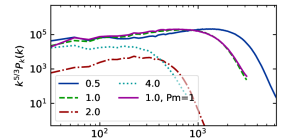
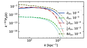
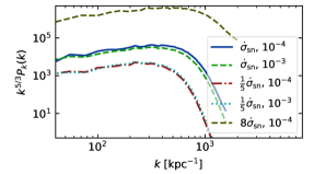
Figure 4: Compensated magnetic (left) and kinetic (right) energy spectra. Compensation is for the Kazantsev spectrum $k^{3/2}$ (left) or the Kolmogorov spectrum $k^{-5/3}$ (right). (a)–(c): Samples at $t=27.5~{}{\rm Myr}$ for ${\delta x}$ given in the legend for resistivity $\eta$ and supernova rate $\dot{\sigma}$ as indicated on each panel. Field strengths reached differ between models at this time (see Fig. 3). Viscosity $\nu=0$, except $\nu=10^{-3}$ for models identified by Pm. (d): Samples taken at different times but similar field strength at $\eta$ and $\dot{\sigma}$ as indicated in the legend, with the highest supernova rate being the ${\delta x}=1.56$ run from the comparison with BKMM4 and ${\delta x}=2$ otherwise.

4 Results

4.1 Resolution and convergence

Figure 3 shows that numerical diffusion still dominates at studied resolutions for resistivity $\eta=10^{-4}$, as can be seen from the increasing speed of the SSD with resolution, but that a converged SSD solution emerges at $\eta=10^{-3}$ for parsec resolution. Saturation at around 5% of $\overline{e_{K}}$ appears to be a well-converged result. The $\eta=10^{-3}$ models show false convergence (Fryxell et al., 1991) of solutions with similar magnetic energy decay at ${\delta x}\geq 2$. We note that strong fluctuations in the characteristics of the flow occur at the low $\dot{\sigma}$ that we choose to avoid thermal runaway (Li et al., 2015), with thermal phases occupying changing fractional volumes (e.g. Gatto et al., 2015) and hosting SSD instabilities with different thresholds and growth rates.

We ran models to reproduce the results of BKMM4, which adopt their choice $\dot{\sigma}=8\dot{\sigma}_{\rm sn}$. In our fiducial runs we use a lower value of $0.2\dot{\sigma}_{\rm sn}$ to preserve multiphase thermal structure. The higher $\dot{\sigma}$ rapidly drives thermal runaway resulting in high temperatures $T>10^{7}$ K. The growth rate is faster than in our fiducial models (Figure 3 (c)), reflective of the single phase kinematics and more persistent forcing rate, yet still saturating at about 5% of $\overline{e_{K}}$. At equivalent resolution, the sixth-order Pencil Code has far lower diffusion than the second-order Godunov code used by BKMM4. As a result, we find faster growth at equivalent resolution. Figure 3(d) shows that kinetic energy fluctuates around a stationary mean in our models, with higher SN rate $\dot{\sigma}$ producing higher kinetic energy, less intermittency in the energy, and less erratic growth in the dynamo.

We can also examine the kinetic and magnetic energy spectra (Figure 4). The kinetic spectra for ${\delta x}\leq 1$ agree well at all scales above the viscous cutoff, which appears, as expected, at lower $k$ for ${\delta x}=1$ than ${\delta x}=0.5$. By contrast the kinetic spectra for ${\delta x}\geq 2$ differ and exhibit significant energy losses at all scales, indicating only solutions for ${\delta x}\lesssim 1$ have converged.

The addition of viscosity $\nu=10^{-3}$, indicated by the magenta curves in panels (b) and (c), makes little difference to the shape of the magnetic or kinetic energy spectra. The magnitude of the magnetic energy spectrum increases somewhat with the addition of viscosity, as can also be seen from comparing dotted light and dark blue lines in Figure 5 (a2).

We have shown that SSD turbulence converges for ${\delta x}\leq 1$. Underresolving SN driven turbulence results in a significant loss of energy at all scales. The SSD for $0.2\dot{\sigma}_{\rm sn}\leq\dot{\sigma}\leq 8\dot{\sigma}_{\rm sn}$ saturates in the ISM at about $5\%\overline{e_{K}}$ and grows more rapidly with increasing SN rate.

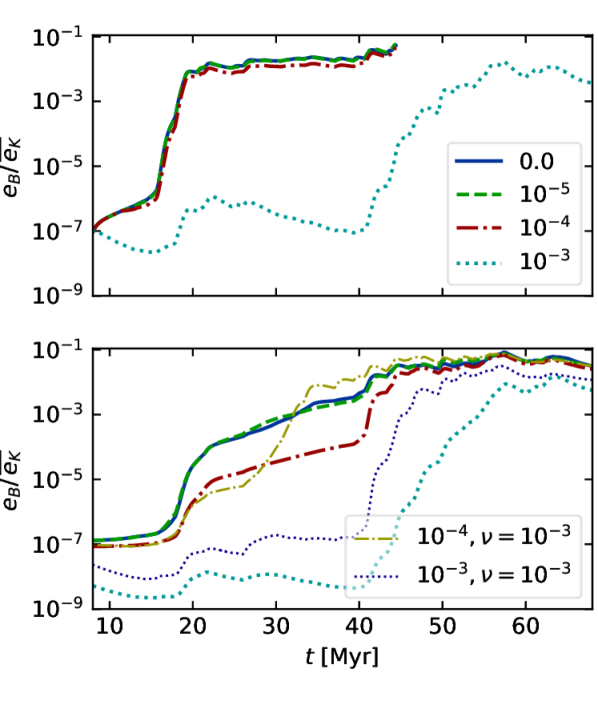
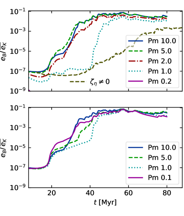
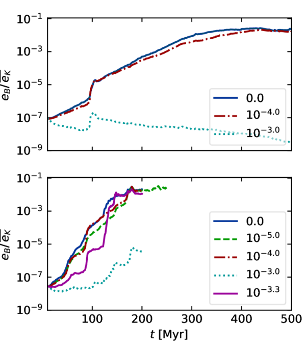
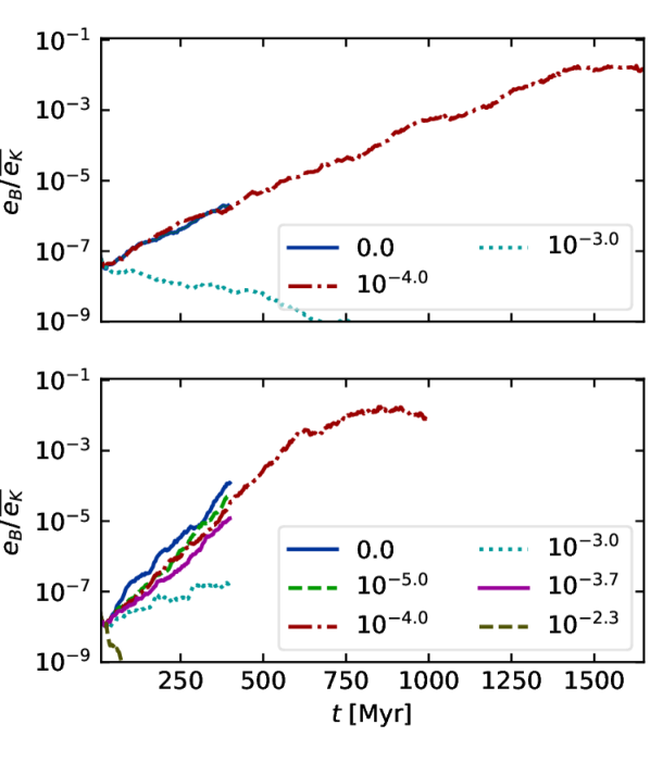
Figure 5: Magnetic energy density $e_{B}$ normalized by the time-averaged kinetic energy $\overline{e_{K}}$ for values given in each panel of resolution ${\delta x}$ and SN rate $\dot{\sigma}$. Time axes extend for ${\delta x}\geq 2$ to accommodate SSD saturation. Captions indicate resistivity $\eta$, with viscosity $\nu=0$, unless indicated otherwise or where ${\rm Pm}=\nu/\eta$ is varied with $\nu$ fixed (b1) or $\eta$ fixed (b2). In (b1) the run with $\zeta_{\eta}=0.55$ has ${\rm Pm}=10$. All other models have $\zeta_{\eta}=0$. Line styles in (a1) also apply in (a2).

4.2 Effective resistivity and Prandtl number

To understand the role of physical resistivity $\eta$ and viscosity $\nu$ on the SSD, we need to determine the value at each resolution where they exceed numerical diffusion in strength. Figure 5 shows that a physical resistivity of $\eta=10^{-5}$ (panels a1, a2) makes no impact on field growth at $\dot{\sigma}=0.2\dot{\sigma}_{\rm sn}$, while $\eta=10^{-3}$ clearly dominates over numerical resistivity at all resolutions. The exact value of the minimum physical resistivity does seem to vary not just with ${\delta x}$ but also with $\sigma$, as can be seen by comparison of the $\eta=10^{-4}$ and $10^{-3}$ cases (panels c1 to d2).

When we consider $e_{B}$ for the models with only numerical viscosity (Fig 5 a, c, d), $\eta\geq 10^{-3}$ initially appears sufficient to suppress SSD. At low resolution this remains so for $\dot{\sigma}=0.2\dot{\sigma}_{\rm sn}$ (panels c1 and d1), apart from a transitory surge near 100 Myr for ${\delta x}=2$. However, for $\dot{\sigma}=\dot{\sigma}_{\rm sn}$ within 100 Myr SSD is evident. Only, $\eta=0.005$ dampens SSD (panel d2).

The kinetic energy spectra in Figure 4 may show the resolution of this contradiction. They display a bottleneck effect (Falkovich, 1994; Haugen et al., 2003), an energy cascade less efficient than $k^{-5/3}$ leading to an accumulation of power and then rapid dissipation at high $k$. This bottleneck shifts to lower $k$ as ${\delta x}$ increases (panels a–c) or $\dot{\sigma}$ decreases (panel d). The deeper into the magnetic energy spectrum this peak extends, the more scales available for transfer to magnetic energy and the more efficient the SSD. The critical resistivity above which SSD is suppressed, therefore, increases with $\dot{\sigma}$, within the range considered. Even at $\dot{\sigma}=0.2$, for $\eta=10^{-3}$ and ${\delta x}\leq 1$ SSD occurs after 20 – 40 Myr.

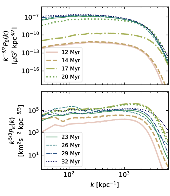
Figure 6: Compensated spectra as in Figure 4 of magnetic (a1, b1) and kinetic (a2, b2) energy at times given in the legends (combined for each pair) for ${\delta x}$, $\dot{\sigma}$ and $\eta$ indicated. Resistivity is $\eta=10^{-4}$ with (b1,b2) a comparison to ${\sf BKMM4}$.

Resistivity contributes to Rm, which is expected to control the onset of the SSD and affect growth rate. We therefore anticipate that lower $\eta$ would correlate with higher growth rate (Schekochihin et al., 2007). This mainly is the case when we compare models with ${\delta x}\leq 1$ at concurrent stages in their evolution. However, in Figure 5 (c2) there are some anomolous patterns, where higher $\eta$ models overtake lower $\eta$ models, e.g., at 80 Myr. To explore this further we include experiments with ${\delta x}=1$ and $\nu>0$, and examine the effect of Pm on the SSD (Figure 5 b1, b2). We identify each model by ${\rm Pm}=\nu/\eta$, but due to the inclusion of shock and hyper diffusivities, the effective Pm and, indeed, Rm vary substantially across space and time. In b1 we include one run with shock resistivity, $\zeta_{\eta}\neq 0$ (olive, dashed), which is referenced in Figure 2. The dynamo is slower and saturates lower than the comparative model ${\rm Pm}=10$ (blue, solid). This is consistent with more efficient dissipation of compressed field.

Plotted in panel b2, where we fix $\eta=10^{-4}$ and vary $\nu$, initial growth of $e_{B}$ is faster for ${\rm Pm}=0.1$ than for higher values. This is a regime less conducive to exciting the SSD than the high ${\rm Pm}$ regime typical of the ISM (Haugen et al., 2004a). A plausible explanation may be that the higher fluid Reynolds number, Re, could facilitate the dynamo. We therefore set a physical viscosity $\nu=10^{-3}$ and vary $\eta$. Plotted in panel (b1) the growth rates mainly conform to our expectations, except for ${\rm Pm}=5$ between 20 and 40 Myr. We confirm that $\eta\geq 10^{-2.3}$ suppresses SSD at $\dot{\sigma}=0.2\dot{\sigma}_{\rm sn}$. While the saturation level is insensitive to Pm, with $\nu$ fixed (panel b2), the saturation level increases with Pm for $\eta$ fixed (panel b1), indicating saturation level is sensitive to Re. We also include two of these plots in panel (a2) for comparison to $\nu=0$. Comparing the kinetic energy spectra (magenta) models in Figure 4 (b2, c2), $\nu$ alters very little.

We have shown that the critical resistivity for SSD in the ISM with a low SN rate is $10^{-2.3}>\eta_{\rm crit}>10^{-3}$ and that this increases with increasing $\dot{\sigma}$ within the range considered. Although higher Rm and Pm generally increase growth rate and saturation in line with theoretical expectations, there is considerable variation, likely due to intermittency in the multiphase ISM.

4.3 Tangling of the imposed field

We now examine whether the field growth seen in our models could be due to tangling. In Sect. 2 we argued that tangling should produce linear growth rate, with dissipation dominating scales below the forcing range. Conversely, an SSD leads to exponential growth and a Kazantsev cascade extending below the forcing scale.

SN-driven turbulence does not have a single forcing scale, because of explosions randomly located in the heterogeneous ISM. Instead, the forcing is distributed at scales of roughly 60–200 pc (Joung & Mac Low, 2006; de Avillez & Breitschwerdt, 2007; Hollins et al., 2017), or $k\sim 30$–105 kpc^-1.

In Figures 3 and 5 we indeed demonstrate strong exponential growth over multiple orders of magnitude for sufficiently low resistivity, at varying supernova rate $\dot{\sigma}$, numerical resolution ${\delta x}$, and physical viscosity $\nu$. Apparently linear growth occurs only with high physical resistivity.

We now turn to the power spectra. Figure 6 shows compensated spectra over time during intervals that span epochs with distinct rates of SSD growth followed by saturation. The compensated magnetic energy spectra in Figure 6 (a1, b1) have peaks conforming to the end of the Kazantsev range.

For ${\dot{\sigma}=0.2\dot{\sigma}_{\rm sn}}$ up to 14 Myr this peak is at $k{\simeq 200}~{}{\rm kpc}^{-1}$ while the SSD grows slowly. During accelerated growth the Kazentsev range extends to $k\gtrsim{700}~{}{\rm kpc}^{-1}$, above the forcing scale and consistent with SSD as shown in the uniform, isothermal model (Fig. 1b). The peak contracts upon saturation to $k<{200}~{}{\rm kpc}^{-1}$, consistent with no further dynamo (Fig. 1c).

In Figure 6 (b1) until 7 Myr there is no Kazantsev range and the peak energy increases as $k\rightarrow 0$, a signature of tangling of the imposed field. However, as the magnetic field grows much larger than the imposed field, this signature disappears and the peak shifts to high $k$, suggesting a healthy SSD.

We have demonstrated that the magnetic field amplification in BKMM4 is due to SSD. Tangling of the imposed field is initially present, but is dominated by SSD. Our other models with only a weak seed field confirm that an imposed field is not required.

5 Conclusions

Through the most extensive resolution and parameter study to date, we demonstrate in this Letter that SSD likely occurs easily in the ISM. The critical resistivity is $0.005>\eta_{\rm crit}\gtrsim 0.001~{}{\rm kpc}~{}{\rm km~{}s}^{-1}$ for supernova rate $\dot{\sigma}=0.2\dot{\sigma}_{\rm sn}$ and increasing over the range considered $\dot{\sigma}\in(0.2\dot{\sigma}_{\rm sn},8\dot{\sigma}_{\rm sn})$. The SSD saturates at about 5% of the equipartition kinetic energy density. This level is insensitive to Pm, but increases with increasing Re. We find that the conventional approach from dynamo theory of categorising the turbulence according to Rm based on a forcing scale $\ell$, mean random velocity $u_{\rm rms}$ and resistivity $\eta$ is inadequate for such a complicated system.

We show that simulations with insufficient resolution can appear to converge to a false solution lacking dynamo activity (Fig. 3b). This can occur because these simulations are not scale independent. The SN energy input and the physically motivated ISM cooling processes impose length and time scales that must be adequately resolved. We obtain convergent results for SSD with grid resolution ${\delta x}\lesssim 1$.

We confirm, by comparing models with and without an imposed magnetic field, that the field amplification obtained in SN-driven ISM turbulence by Balsara et al. (2004) was evidence of an SSD and not only due to tangling of their imposed field. A seed field of less than 1 nG can be amplified to saturation at microgauss levels within about 10 Myr (Figure 3).

Gressel et al. (2008) and Gressel & Elstner (2020) have ${\delta x}=8.3$ and $6.7~{}{\rm pc}$, respectively, and $\eta\simeq 10^{-2.2}~{}{\rm kpc}~{}{\rm km~{}s}^{-1}$, which appears to exclude an SSD. Gent et al. (2013b) with ${\delta x}=4~{}{\rm pc}$ applied $\eta\simeq 10^{-3.1}~{}{\rm kpc}~{}{\rm km~{}s}^{-1}$, which would support SSD for $\dot{\sigma}\simeq\dot{\sigma}_{\rm sn}$. We can now construct LSD experiments to explore how SSD impacts the onset of LSD, critical $\Omega$, and dependence on $\dot{\sigma}$.

References

- Balsara & Kim (2005) Balsara, D. S., & Kim, J. 2005, ApJ, 634, 390
- Balsara et al. (2004) Balsara, D. S., Kim, J., Mac Low, M.-M., & Mathews, G. J. 2004, ApJ, 617, 339
- Begelman & McKee (1990) Begelman, M. C., & McKee, C. F. 1990, ApJ, 358, 375
- Bhat & Subramanian (2014) Bhat, P., & Subramanian, K. 2014, ApJ, 791, L34
- Brandenburg & Dobler (2002) Brandenburg, A., & Dobler, W. 2002, Computer Physics Communications, 147, 471
- Brandenburg & Sarson (2002) Brandenburg, A., & Sarson, G. R. 2002, Phys. Rev. Lett., 88, 055003
- Brandenburg et al. (2020) Brandenburg, A., Johansen, A., Bourdin, P. A., et al. 2020, arXiv e-prints, arXiv:2009.08231
- de Avillez & Breitschwerdt (2005) de Avillez, M. A., & Breitschwerdt, D. 2005, A&A, 436, 585
- de Avillez & Breitschwerdt (2007) —. 2007, ApJ, 665, L35
- Evirgen et al. (2017) Evirgen, C. C., Gent, F. A., Shukurov, A., Fletcher, A., & Bushby, P. 2017, MNRAS, 464, L105
- Falkovich (1994) Falkovich, G. 1994, Physics of Fluids, 6, 1411
- Federrath et al. (2011) Federrath, C., Chabrier, G., Schober, J., et al. 2011, Phys. Rev. Lett., 107, 114504
- Federrath et al. (2014) Federrath, C., Schober, J., Bovino, S., & Schleicher, D. R. G. 2014, ApJ, 797, L19
- Fryxell et al. (1991) Fryxell, B., Mueller, E., & Arnett, D. 1991, ApJ, 367, 619
- Gatto et al. (2015) Gatto, A., Walch, S., Mac Low, M.-M., et al. 2015, MNRAS, 449, 1057
- Gent et al. (2020) Gent, F. A., Mac Low, M.-M., Käpylä, M. J., Sarson, G. R., & Hollins, J. F. 2020, Geophysical and Astrophysical Fluid Dynamics, 114, 77
- Gent et al. (2013a) Gent, F. A., Shukurov, A., Fletcher, A., Sarson, G. R., & Mantere, M. J. 2013a, MNRAS, 432, 1396
- Gent et al. (2013b) Gent, F. A., Shukurov, A., Sarson, G. R., Fletcher, A., & Mantere, M. J. 2013b, MNRAS, 430, L40
- Gressel & Elstner (2020) Gressel, O., & Elstner, D. 2020, MNRAS, 494, 1180
- Gressel et al. (2008) Gressel, O., Ziegler, U., Elstner, D., & Rüdiger, G. 2008, Astronomische Nachrichten, 329, 619
- Hanasz et al. (2009) Hanasz, M., Wóltański, D., & Kowalik, K. 2009, ApJ, 706, L155
- Haugen et al. (2004a) Haugen, N. E., Brandenburg, A., & Dobler, W. 2004a, Phys. Rev. E, 70, 016308
- Haugen & Brandenburg (2004) Haugen, N. E. L., & Brandenburg, A. 2004, Phys. Rev. E, 70, 036408
- Haugen et al. (2003) Haugen, N. E. L., Brandenburg, A., & Dobler, W. 2003, ApJ, 597, L141
- Haugen et al. (2004b) Haugen, N. E. L., Brandenburg, A., & Mee, A. J. 2004b, MNRAS, 353, 947
- Hennebelle & Iffrig (2014) Hennebelle, P., & Iffrig, O. 2014, A&A, 570, A81
- Hill et al. (2012) Hill, A. S., Joung, M. R., Mac Low, M.-M., et al. 2012, ApJ, 750, 104
- Hollins et al. (2017) Hollins, J. F., Sarson, G. R., Shukurov, A., Fletcher, A., & Gent, F. A. 2017, ApJ, 850, 4
- Joung & Mac Low (2006) Joung, M. K. R., & Mac Low, M.-M. 2006, ApJ, 653, 1266
- Korpi et al. (1999) Korpi, M. J., Brandenburg, A., Shukurov, A., & Tuominen, I. 1999, A&A, 350, 230
- Li et al. (2015) Li, M., Ostriker, J. P., Cen, R., Bryan, G. L., & Naab, T. 2015, ApJ, 814, 4
- Mac Low et al. (2005) Mac Low, M.-M., Balsara, D. S., Kim, J., & de Avillez, M. A. 2005, ApJ, 626, 864
- Pakmor et al. (2017) Pakmor, R., Gómez, F. A., Grand , R. J. J., et al. 2017, MNRAS, 469, 3185
- Piontek & Ostriker (2007) Piontek, R. A., & Ostriker, E. C. 2007, ApJ, 663, 183
- Rieder & Teyssier (2016) Rieder, M., & Teyssier, R. 2016, MNRAS, 457, 1722
- Sarazin & White (1987) Sarazin, C. L., & White, III, R. E. 1987, ApJ, 320, 32
- Schekochihin et al. (2002) Schekochihin, A. A., Boldyrev, S. A., & Kulsrud, R. M. 2002, ApJ, 567, 828
- Schekochihin et al. (2007) Schekochihin, A. A., Iskakov, A. B., Cowley, S. C., et al. 2007, New Journal of Physics, 9, 300
- Steinwandel et al. (2019) Steinwandel, U. P., Beck, M. C., Arth, A., et al. 2019, MNRAS, 483, 1008
- Wang & Abel (2009) Wang, P., & Abel, T. 2009, ApJ, 696, 96
- Wolfire et al. (1995) Wolfire, M. G., Hollenbach, D., McKee, C. F., Tielens, A. G. G. M., & Bakes, E. L. O. 1995, ApJ, 443, 152
- Zeldovich et al. (1983) Zeldovich, Y. B., Ruzmaikin, A. A., & Sokolov, D. D. 1983, Magnetic fields in astrophysics (Gordon & Breach, New York)