UMTG–309

Bethe ansatz on a quantum computer?
Rafael I. Nepomechie
Physics Department, P.O. Box 248046
University of Miami, Coral Gables, FL 33124

We consider the feasibility of studying the anisotropic Heisenberg quantum spin chain with the Variational Quantum Eigensolver (VQE) algorithm, by treating Bethe states as variational states, and Bethe roots as variational parameters. For short chains, we construct exact one-magnon trial states that are functions of the variational parameter, and implement the VQE calculations in Qiskit. However, exact multi-magnon trial states appear to be out out of reach.

1 Introduction

Significant attention is being focused on an algorithm in quantum computing known as the Variational Quantum Eigensolver (VQE) [1, 2, 3] . In the era of Noisy Intermediate-Scale Quantum devices [4], this algorithm may have practical applications in quantum chemistry [5, 6, 7]. The basic idea is to reduce the chemistry problem to a one-dimensional quantum spin chain Hamiltonian, whose ground-state energy is then estimated using the variational principle by means of a hybrid quantum/classical computation. A nice feature of this approach is that the Hamiltonian does not need to be implemented in a circuit. The main challenge is to find a suitable variational state, which typically depends on many variational parameters.

It has long been known that certain one-dimensional quantum spin chains are integrable, and can therefore be “solved exactly” by Bethe ansatz [8]. Indeed, the eigenstates have a general form (Bethe states) that depend on a set of parameters (Bethe roots), which obey a set of equations called Bethe equations; however, these equations are in general hard to solve. Because of the relative simplicity of such Bethe-ansatz-solvable spin chains compared with those arising in quantum chemistry, the former could serve as useful testbeds of the VQE approach. (Simpler integrable models have been studied on quantum computers using other methods, see e.g. [9] and references therein.)

We consider here the feasibility of studying Bethe-ansatz-solvable spin chains with VQE, by treating Bethe states as variational states, and Bethe roots as variational parameters. Attractive features of this idea are that the variational states can become exact, and that the number of Bethe roots scales linearly with the length of the chain.

We find that such an approach is indeed feasible for short chains, which however can be easily solved by elementary means. But for longer chains, this approach does not seem feasible, due to the difficulty of constructing the variational states.

The outline of this paper is as follows. In Sec. 2, we introduce the model, and set up a variational problem using one-magnon trial states. We discuss the cases of 2 and 4 sites, including their implementations in Qiskit [10, 11] using the IBM Quantum Experience [12], in Secs. 3 and 4, respectively. We briefly discuss multi-magnon states in Sec. 5, and draw some conclusions in Sec. 6. The needed Bethe ansatz results are collected in Appendix A.

2 The model

We consider as our working example the periodic spin-1/2 anisotropic Heisenberg (XXZ) quantum spin chain with $N$ sites in the ferromagnetic regime, whose Hamiltonian is given by

$${\cal H}=-\frac{1}{4}\sum_{k=1}^{N}\left[\sigma^{x}_{k}\sigma^{x}_{k+1}+\sigma^{y}_{k}\sigma^{y}_{k+1}+\cosh(\eta)\left(\sigma^{z}_{k}\sigma^{z}_{k+1}-\sigma^{0}_{k}\sigma^{0}_{k+1}\right)\right]\,,\qquad\sigma^{i}_{N+1}\equiv\sigma^{i}_{1}\,,$$ (2.1)

where $\sigma^{i}_{k}$ denotes the $i^{th}$ Pauli matrix at site $k$ ($\sigma^{0}$ is the two-dimensional identity matrix), and $\eta>0$ is the anisotropy parameter. This model and its cousins have a long history, and have applications ranging from condensed matter physics and statistical mechanics to high-energy theory [13].

This model has a $U(1)$ symmetry

$$\left[{\cal H}\,,S^{z}\right]=0\,,\qquad S^{z}=\frac{1}{2}\sum_{k=1}^{N}\sigma^{z}_{k}\,,$$ (2.2)

as well as charge conjugation symmetry

$${\cal C}\,{\cal H}\,{\cal C}={\cal H}\,,\qquad{\cal C}=\prod_{k=1}^{N}\sigma^{x}_{k}\,.$$ (2.3)

Note that ${\cal C}\,S^{z}\,{\cal C}=-S^{z}$. Hence, if $|\Psi\rangle$ is a simultaneous eigenstate of ${\cal H}$ and $S^{z}$ with nonzero eigenvalue of $S^{z}$, then it is degenerate, since ${\cal C}\,|\Psi\rangle$ has the same energy as (and is linearly independent from) $|\Psi\rangle$.

Let $|\Psi_{0}\rangle$ denote the reference state

$$|\Psi_{0}\rangle={1\choose 0}^{\otimes N}\,.$$ (2.4)

Both $|\Psi_{0}\rangle$ and ${\cal C}|\Psi_{0}\rangle$ are ground states of the Hamiltonian (2.1), with energy 0 and $S^{z}$ eigenvalues $N/2$ and $-N/2$ respectively.

Our initial (admittedly, modest) objective is to use VQE to estimate the energy of the first excited state. The normalized trial state $|\Psi\rangle$ must be orthogonal to both ground states

$$\langle\Psi_{0}|\Psi\rangle=\langle\Psi_{0}|{\cal C}|\Psi\rangle=0\,.$$ (2.5)

Indeed, the usual variational argument can then be applied: let $\{|n\rangle\}$ be a complete orthonormal set of eigenstates of the Hamiltonian (2.1)

$${\cal H}\,|n\rangle=E_{n}\,|n\rangle\,,\qquad\langle n|m\rangle=\delta_{n,m}\,,\qquad\sum_{n=0}^{2^{N}-1}|n\rangle\langle n|=1\,,$$ (2.6)

with ordered energies $E_{n}\leq E_{n+1}$. The requirement (2.5) translates to

$$\langle n|\Psi\rangle=0\,,\qquad n=0,1\,.$$ (2.7)

We then have

$$1=\langle\Psi|\Psi\rangle=\sum_{n=0}^{2^{N}-1}|\langle n|\Psi\rangle|^{2}=\sum_{n=2}^{2^{N}-1}|\langle n|\Psi\rangle|^{2}$$ (2.8)

and

$$\langle\Psi|{\cal H}|\Psi\rangle =\sum_{m,n=0}^{2^{N}-1}\langle\Psi|m\rangle\langle m|{\cal H}|n\rangle\langle n|\Psi\rangle=\sum_{n=0}^{2^{N}-1}E_{n}|\langle n|\Psi\rangle|^{2}=\sum_{n=2}^{2^{N}-1}E_{n}|\langle n|\Psi\rangle|^{2}$$

$$=E_{2}+\sum_{n=3}^{2^{N}-1}(E_{n}-E_{2})|\langle n|\Psi\rangle|^{2}\geq E_{2}\,.$$ (2.9)

That is, the expectation value of the Hamiltonian in the trial state is greater than or equal to the energy of the first excited state.

We take as our trial state the so-called one-magnon Bethe state

$$|\Psi\rangle=\frac{|\psi\rangle}{\sqrt{\langle\psi|\psi\rangle}}\,,\qquad|\psi\rangle=B(p)|\Psi_{0}\rangle\,,$$ (2.10)

where the operator $B(p)$, which is not unitary, is defined in Appendix A. The requirement (2.5) can be shown to be satisfied (for $N>1$) by using the facts

$$\langle\Psi_{0}|B(p)=0$$ (2.11)

and

$$\left[S^{z}\,,B(p)\right]=-B(p)\,.$$ (2.12)

Indeed, from (2.11), we see that

$$\langle\Psi_{0}|\psi\rangle=\langle\Psi_{0}|B(p)|\Psi_{0}\rangle=0\,;$$ (2.13)

and from (2.12), we obtain

$$\langle\Psi_{0}|{\cal C}\left[S^{z}\,,B(p)\right]|\Psi_{0}\rangle=-\langle\Psi_{0}|{\cal C}B(p)|\Psi_{0}\rangle\,,$$ (2.14)

whose left-hand-side can be evaluated as follows:

$$\langle\Psi_{0}|{\cal C}\left[S^{z}\,,B(p)\right]|\Psi_{0}\rangle =\langle\Psi_{0}|\left({\cal C}S^{z}B(p)-{\cal C}B(p)S^{z}\right)|\Psi_{0}\rangle$$ (2.15)

$$=\langle\Psi_{0}|\left(-S^{z}{\cal C}B(p)-{\cal C}B(p)S^{z}\right)|\Psi_{0}\rangle$$ (2.16)

$$=-N\langle\Psi_{0}|{\cal C}B(p)|\Psi_{0}\rangle\,.$$ (2.17)

In passing to (2.16), we have used the fact (noted below (2.3)) that ${\cal C}\,S^{z}\,{\cal C}=-S^{z}$; and in passing to (2.17), we have used the fact $S^{z}|\Psi_{0}\rangle=(N/2)|\Psi_{0}\rangle$, which follows from the remark below (A.10). In view of (2.14), we see that

$$(N-1)\langle\Psi_{0}|{\cal C}B(p)|\Psi_{0}\rangle=0\,.$$ (2.18)

Hence, for $N>1$, we conclude that

$$\langle\Psi_{0}|{\cal C}|\psi\rangle=\langle\Psi_{0}|{\cal C}B(p)|\Psi_{0}\rangle=0\,.$$ (2.19)

Eqs. (2.13) and (2.19) imply that the trial state (2.10) is orthogonal to both ground states. (For other approaches to studying excited states using VQE, see e.g. [14, 15].)

Note that, as a consequence of (2.12), the trial state (2.10) has $S^{z}$ eigenvalue $(N/2)-1$. Note also that the trial state depends on a single variational parameter $p$, which we take to be real. The cases $N=2$ and $N=4$ are explicitly worked out in Secs. 3 and 4, respectively.

3 $N=2$

We begin with the simplest case of 2 sites, for which there are 4 states: the two zero-energy ground states $|\Psi_{0}\rangle$ and ${\cal C}|\Psi_{0}\rangle$, and the first and second excited states. By direct diagonalization of the Hamiltonian (2.1), one finds that the excited states have energies $\cosh(\eta)-1$ and $\cosh(\eta)+1$, respectively. We shall see that in fact both excited-state energies can be obtained using VQE.

The trial state (2.10) is given for $N=2$ by

$$|\Psi\rangle=\frac{1}{\sqrt{2}}(0,e^{ip},1,0)\,,$$ (3.1)

up to an overall phase. In order to implement VQE, we must first re-express this state as a product of standard 1-qubit and 2-qubit unitary gates acting on the reference state $|\Psi_{0}\rangle$. Up to an overall phase, we find that

$$|\Psi\rangle=X_{0}\,C_{10}\,U^{(3)}_{1}(\tfrac{\pi}{2},-p,0)\,|\Psi_{0}\rangle\,,$$ (3.3)

where $X=\sigma^{x}$, $C_{ij}$ is a CNOT gate with control qubit $i$ and target qubit $j$

$$C_{10}=\begin{pmatrix}1&0&0&0\\ 0&1&0&0\\ 0&0&0&1\\ 0&0&1&0\end{pmatrix}\,,$$ (3.4)

and $U^{(3)}(\theta,\phi,\lambda)$ is defined by

$$U^{(3)}(\theta,\phi,\lambda)=\begin{pmatrix}\cos(\theta/2)&-e^{i\lambda}\sin(\theta/2)\\ e^{i\phi}\sin(\theta/2)&e^{i\phi}e^{i\lambda}\cos(\theta/2)\end{pmatrix}\,.$$ (3.5)

The exact energy of the first-excited state can be obtained by minimizing $\langle\Psi|{\cal H}|\Psi\rangle=\cosh(\eta)-\cos(p)$; the corresponding optimal value of the variational parameter is $p=0\,\,(\text{mod}\,\,2\pi)$, independently of the value of $\eta$.

For $N=2$, the second-excited state also has the one-magnon form (3.1), see Appendix A. Since this state is in fact the state with highest energy, we can obtain its energy via VQE by minimizing $\langle\Psi|(-{\cal H})|\Psi\rangle=\cos(p)-\cosh(\eta)$, and then taking the absolute value of the result. The corresponding optimal value of the variational parameter in this case is $p=\pi\,\,(\text{mod}\,\,2\pi)$.

3.1 Qiskit implementation

We implemented these variational computations in Qiskit using its VQE algorithm, which iteratively evaluated $\langle\Psi|{\cal H}|\Psi\rangle$, using a classical optimizer to update the value of $p$. We inputted the Hamiltonian (2.1) as a 2-qubit SummedOp, and used the Constrained Optimization By Linear Approximation (COBYLA) as the classical optimizer (maxiter=10). The circuit diagram for the trial state $|\Psi\rangle$ given by (3.3) is shown in Fig. 1. For concreteness, we set $\eta=1$. Typical results, together with the exact result, are presented in Table 1. The results from the real device ibmq_valencia (5 qubits, QV16), using measurement error mitigation, have error of approximately $1\%$.

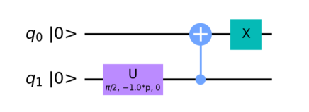
Figure 1: Circuit for the trial state $|\Psi\rangle$ given by (3.3)

Backend	$E_{\text{first-excited state}}$	$p\,\,(\text{mod}\,\,2\pi)$	$E_{\text{second-excited state}}$	$p\,\,(\text{mod}\,\,2\pi)$
Exact	0.54308063	0	2.54308063	3.14159265
Statevector simulator	0.54316139	-0.01270853	2.54203089	-3.09576858
Qasm simulator ($10^{3}$ shots, no noise)	0.54308063	-0.01549807	2.54308063	3.17170765
Real 5-qubit device ($10^{3}$ shots)	0.54549027	-0.17336981	2.54191949	2.97042731

Table 1: VQE energies and optimal parameter values for the Hamiltonian (2.1) with $N=2$ and $\eta=1$, using the trial state depicted in Fig. 1

4 $N=4$

We now consider the case of 4 sites. By direct diagonalization of the Hamiltonian (2.1), one finds that the exact energy of the (two-fold degenerate) first-excited states is $\cosh(\eta)-1$.

The trial state (2.10) is now given by

$$|\Psi\rangle=(0,\tfrac{1}{2}e^{3ip/2},\tfrac{1}{2}e^{ip/2},0,\tfrac{1}{2}e^{-ip/2},0,0,0,\tfrac{1}{2}e^{-3ip/2},0,0,0,0,0,0,0)\,,$$ (4.1)

up to an overall phase. The main difficulty is to re-express this state as a product of standard 1-qubit and 2-qubit unitary gates acting on the reference state $|\Psi_{0}\rangle$. To this end, we follow [16], and perform the Schmidt decomposition of (4.1), thereby obtaining

$$|\Psi\rangle=\left({\cal U}\otimes{\cal V}\right)C_{31}\,C_{20}\,H_{2}\,|\Psi_{0}\rangle\,,$$ (4.2)

where $H$ is the Hadamard gate

$$H=\frac{1}{\sqrt{2}}\begin{pmatrix}1&1\\ 1&-1\end{pmatrix}\,,$$ (4.3)

and ${\cal U}$ and ${\cal V}$ are the following unitary matrices

$${\cal U}=\begin{pmatrix}e^{ip/2}&0&0&0\\ 0&\frac{1}{\sqrt{2}}e^{-ip/2}&0&-\frac{1}{\sqrt{2}}e^{ip}\\ 0&\frac{1}{\sqrt{2}}e^{-3ip/2}&0&\frac{1}{\sqrt{2}}\\ 0&0&1&0\end{pmatrix}\,,\qquad{\cal V}=\begin{pmatrix}0&1&0&0\\ \frac{1}{\sqrt{2}}e^{ip}&0&0&-\frac{1}{\sqrt{2}}e^{ip}\\ \frac{1}{\sqrt{2}}&0&0&\frac{1}{\sqrt{2}}\\ 0&0&1&0\end{pmatrix}\,.$$ (4.4)

We now need to decompose ${\cal U}$ and ${\cal V}$ into gates. To this end, we follow [17, 18, 19], and eventually obtain (up to irrelevant overall phases)

$${\cal U} =\left[U^{(3)}(\tfrac{\pi}{2},-\tfrac{3p}{2},0)\otimes U^{(3)}(\tfrac{\pi}{2},\tfrac{1}{2}(\pi-p),\pi)\right]\,V(0,\tfrac{\pi}{2},\tfrac{\pi}{4})\,$$

$$\qquad\times\left[U^{(3)}(\tfrac{\pi}{2},-\tfrac{\pi}{4},\tfrac{1}{2}(3p+\pi))\otimes U^{(3)}(0,0,\tfrac{1}{2}(3\pi-p))\right]$$ (4.5)

$${\cal V} =\left[U^{(3)}(\tfrac{\pi}{2},\tfrac{1}{2}(\pi-p),0)\otimes U^{(3)}(\tfrac{\pi}{2},\tfrac{p}{2},-\tfrac{\pi}{2})\right]\,V(\tfrac{1}{2}(3\pi-p),\tfrac{3\pi}{4},\tfrac{3\pi}{4})\,$$

$$\qquad\times\left[U^{(3)}(\tfrac{\pi}{2},-\tfrac{\pi}{2},\tfrac{\pi}{2})\otimes U^{(3)}(\tfrac{\pi}{2},-\tfrac{\pi}{2},-\pi)\right]\,,$$ (4.6)

where $V(\alpha,\beta,\delta)$ is the 2-qubit operator defined as

$$V(\alpha,\beta,\delta)=Z_{1}\,C_{01}\,U^{(3)}_{0}(-\alpha,\pi,\pi)\,C_{10}\,U^{(3)}_{1}(0,0,\delta)\,U^{(3)}_{0}(-\beta,\pi,\pi)\,C_{01}\,U^{(3)}_{0}(0,0,-\frac{\pi}{2})\,,$$ (4.7)

with $Z=\sigma^{z}$.

The exact energy of the first-excited states can be obtained by minimizing $\langle\Psi|{\cal H}|\Psi\rangle=\cosh(\eta)-\cos^{3}(p)$; the corresponding optimal value of the variational parameter is $p=0\,\,(\text{mod}\,\,2\pi)$.

4.1 Qiskit implementation

We have again implemented the variational computation in Qiskit using its VQE algorithm with the COBYLA classical optimizer (maxiter=20), inputting the Hamiltonian (2.1) as a 4-qubit SummedOp. We again set $\eta=1$. Circuit diagrams for the trial state $|\Psi\rangle$ (4.2), as well as for the matrices ${\cal U}$ (4.5) and ${\cal V}$ (4.6), are shown in Figs. 2, 3 and 4, respectively. Typical results, together with the exact result, are presented in Table 2. The results from the real device ibmq_santiago (5 qubits, QV32), using measurement error mitigation, have error of approximately $35\%$.

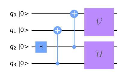
Figure 2: Circuit for the trial state $|\Psi\rangle$ given by (4.2)

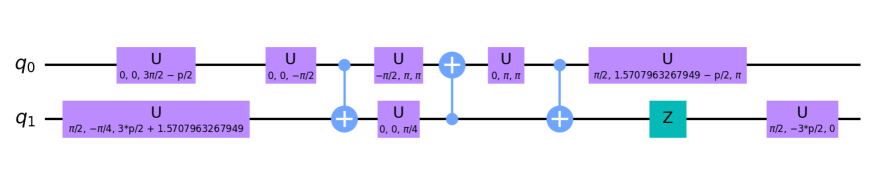
Figure 3: Circuit for the matrix ${\cal U}$ given by (4.5)

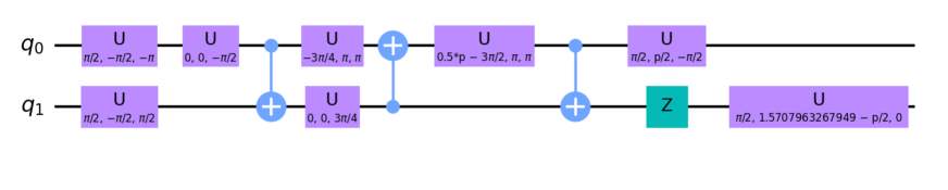
Figure 4: Circuit for the matrix ${\cal V}$ given by (4.6)

Backend	$E_{\text{first-excited states}}$	$p\,\,(\text{mod}\,\,2\pi)$
Exact	0.54308063	0
Statevector simulator	0.54308065	-0.00008658
Qasm simulator ($8192$ shots, no noise)	0.53905231	0.05466209
Real 5-qubit device ($8192$ shots)	0.73343292	0.13868187

Table 2: VQE energy and optimal parameter value for the Hamiltonian (2.1) with $N=4$ and $\eta=1$, using the trial state depicted in Figs. 2-4

5 Multi-magnon states

We have thus far focused on a special class of eigenstates of the Hamiltonian (2.1) described by 1-magnon states (2.10), with $p$ real. However, in order to describe all the eigenstates, it is necessary to consider $M$-magnon states, with $M=0,1,\ldots,\lfloor N/2\rfloor$, and with complex-valued $p$’s. In particular, already for $N=4$, we need also 2-magnon states. Restricting to real values of $p_{1}$ and $p_{2}$ (which is the case for the ground state of $-{\cal H}$), one can show that

$$B(p_{1})\,B(p_{2})|\Psi_{0}\rangle\propto(0,0,0,e^{i(p_{1}+p_{2})},0,\xi,1,0,0,\zeta,\xi^{*},0,e^{-i(p_{1}+p_{2})},0,0,0)\,,$$ (5.1)

where

$$\xi =\frac{1}{1+e^{-i(p_{1}+p_{2})}}\left[e^{ip_{1}}+e^{-ip_{1}}+e^{ip_{2}}+e^{-ip_{2}}-2\cosh(\eta)\right]\,,$$

$$\zeta =\frac{1}{1+e^{i(p_{1}+p_{2})}}\left[1+e^{2ip_{1}}+e^{2ip_{2}}+e^{i(p_{1}-p_{2})}+e^{i(p_{2}-p_{1})}+e^{i(p_{1}+p_{2})}-2\cosh(\eta)(e^{ip_{1}}+e^{ip_{2}})\right]\,,$$ (5.2)

and $\xi^{*}$ denotes the complex conjugate of $\xi$. Unfortunately, we are unable to find an explicit gate decomposition of the corresponding normalized state, since the Schmidt decomposition involves square roots of complicated functions of $p_{1}$, $p_{2}$ and $\eta$. Evidently, exact multi-magnon trial states as explicit functions of the variational parameters are out of reach.

6 Conclusions

We have explicitly derived one-magnon trial states describing the first-excited states of the Hamiltonian (2.1) for the cases $N=2$ and $N=4$, see (3.3) and (4.2)-(4.7), respectively. The main lesson from these computations is that it is possible to obtain gate decompositions of exact one-magnon states that are explicit functions of a variational parameter $p$. We expect that, with additional effort, similar gate decompositions of exact one-magnon states could also be derived for higher values of $N$. However, the corresponding energies of this special class of states can be obtained much more easily by alternative means.

The full power of Bethe ansatz comes from the fact that all eigenstates can be described by multi-magnon states. In principle, this fact could be exploited within the VQE context by using multi-magnon trial states to find the minimum eigenvalue of the antiferromagnetic Hamiltonian $-{\cal H}$, whose ground state lies in the sector with $N/2$ magnons. For $N=2$, the antiferromagnetic ground state is a 1-magnon state, which was already studied in Sec. 3. For $N\geq 4$, the antiferromagnetic ground state lies in a sector with 2 or more magnons. However, as argued in Sec. 5, exact multi-magnon trial states appear to be out of reach. We conclude that a VQE approach based on exact multi-magnon trial states that are explicit functions of the variational parameters does not seem feasible.

One alternative strategy could be to determine the gate decomposition of the exact multi-magnon trial state dynamically. That is, to (classically) recompute the gate decomposition at each stage of the VQE iteration, where the variational parameters have explicit numerical values. Another alternative strategy could be to look for good approximate multi-magnon trial states. We leave these and related questions for future investigations.

Appendix A Bethe ansatz

We collect here the basic results from algebraic Bethe ansatz that are needed to construct the Hamiltonian and trial states. For further details, see e.g. [20, 21, 22]

We start from the (shifted) R-matrix $\mathbb{R}(v)$ acting on $V\otimes V$

$$\mathbb{R}(v)=\begin{pmatrix}\sin(v+\tfrac{i\eta}{2})&0&0&0\\ 0&\sin(v-\tfrac{i\eta}{2})&i\sinh(\eta)&0\\ 0&i\sinh(\eta)&\sin(v-\tfrac{i\eta}{2})&0\\ 0&0&0&\sin(v+\tfrac{i\eta}{2})\end{pmatrix}\,,$$ (A.1)

which is proportional to the permutation matrix (3.2) when $v=\tfrac{i\eta}{2}$, and which is a solution of the (shifted) Yang-Baxter equation on $V\otimes V\otimes V$

$$\mathbb{R}_{12}(v_{1}-v_{2}+\tfrac{i\eta}{2})\,\mathbb{R}_{13}(v_{1})\,\mathbb{R}_{23}(v_{2})=\mathbb{R}_{23}(v_{2})\,\mathbb{R}_{13}(v_{1})\,\mathbb{R}_{12}(v_{1}-v_{2}+\tfrac{i\eta}{2})\,.$$ (A.2)

We define the monodromy matrix $\mathbb{T}_{0}(v)$ by

$$\mathbb{T}_{0}(v)=\mathbb{R}_{0N}(v)\,\ldots\mathbb{R}_{01}(v)\,.$$ (A.3)

This is a matrix acting on $V^{\otimes(N+1)}$; the vector space 0 is called “auxiliary”, and the vector spaces $1,\ldots,N$ are called “quantum”; it is customary to suppress the quantum subscripts of the monodromy matrix. By tracing over the auxiliary space, we arrive at the transfer matrix $\mathbbm{t}(v)$

$$\mathbbm{t}(v)=\mathop{\rm tr}\nolimits_{0}\mathbb{T}_{0}(v)\,,$$ (A.4)

which obeys (as a consequence of the Yang-Baxter equation (A.2)) the commutativity property

$$\left[\mathbbm{t}(v_{1})\,,\mathbbm{t}(v_{2})\right]=0\,,$$ (A.5)

which is the hallmark of quantum integrability. The transfer matrix is the generating function of the Hamiltonian (2.1)

$${\cal H}=-\frac{i}{2}\sinh(\eta)\frac{d}{dv}\log\left(\mathbbm{t}(v)\right)\Big{|}_{v=\frac{i\eta}{2}}+\frac{1}{2}N\cosh(\eta)$$ (A.6)

and of higher conserved commuting quantities.

To construct the eigenstates, we write the monodromy matrix (A.3) as a $2\times 2$ matrix in the auxiliary space

$$\mathbb{T}_{0}(v)=\begin{pmatrix}\mathbb{A}(v)&\mathbb{B}(v)\\ \mathbb{C}(v)&\mathbb{D}(v)\end{pmatrix}_{0}\,,$$ (A.7)

and use the quantum-space operator $\mathbb{B}(v)$ as a creation operator acting on the reference state (2.4). Indeed, it can be shown that the Bethe states

$$\mathbb{B}(v_{1})\ldots\mathbb{B}(v_{M})|\Psi_{0}\rangle$$ (A.8)

are eigenstates of the transfer matrix (and, therefore, of the Hamiltonian) if $v_{1},\ldots,v_{M}$ are pairwise distinct and satisfy the Bethe equations

$$\left(\frac{\sin(v_{j}+\tfrac{i\eta}{2})}{\sin(v_{j}-\tfrac{i\eta}{2})}\right)^{N}=\prod_{k=1;k\neq j}^{M}\frac{\sin(v_{j}-v_{k}+i\eta)}{\sin(v_{j}-v_{k}-i\eta)}\,,\qquad j=1,\ldots,M\,.$$ (A.9)

We can take advantage of the charge conjugation symmetry (2.3) to restrict the values of $M$ to $M=0,1,\ldots,\lfloor N/2\rfloor$. The corresponding eigenvalues of the Hamiltonian are given by

$$E=\frac{1}{2}\sum_{j=1}^{M}\frac{1}{\sin(v_{j}+\tfrac{i\eta}{2})\,\sin(v_{j}-\tfrac{i\eta}{2})}\,.$$ (A.10)

The Bethe states are also eigenstates of $S^{z}$ (2.2), with eigenvalue $(N/2)-M$. We emphasize that the Bethe equations (A.9) cannot be solved analytically unless either the number of sites $N$ or the number of magnons $M$ is very small. In general, one can only solve these equations numerically, and even this is generally very difficult.

It is convenient to change from the variable $v$ to the new variable $p$ defined by

$$\frac{\sin(v+\tfrac{i\eta}{2})}{\sin(v-\tfrac{i\eta}{2})}=e^{-ip}\,,$$ (A.11)

as suggested by the LHS of the Bethe equations (A.9); and we set $B(p)\equiv\mathbb{B}(v)$.

References

- [1] A. Peruzzo, J. McClean, P. Shadbolt, M.-H. Yung, X.-Q. Zhou, P. J. Love, A. Aspuru-Guzik, and J. L. O’Brien, “A variational eigenvalue solver on a photonic quantum processor,” Nature Comm. 5 no. 1, (Jul, 2014) 4213, arXiv:1304.3061 [quant-ph].
- [2] J. R. McClean, J. Romero, R. Babbush, and A. Aspuru-Guzik, “The theory of variational hybrid quantum-classical algorithms,” New J. Phys. 18 no. 2, (Feb, 2016) 023023, arXiv:1509.04279 [quant-ph].
- [3] Y. Alexeev, D. Bacon, K. R. Brown, R. Calderbank, L. D. Carr, F. T. Chong, B. DeMarco, D. Englund, E. Farhi, B. Fefferman, A. V. Gorshkov, A. Houck, J. Kim, S. Kimmel, M. Lange, S. Lloyd, M. D. Lukin, D. Maslov, P. Maunz, C. Monroe, J. Preskill, M. Roetteler, M. Savage, and J. Thompson, “Quantum computer systems for scientific discovery,” arXiv:1912.07577 [quant-ph].
- [4] J. Preskill, “Quantum Computing in the NISQ era and beyond,” Quantum 2 (Aug, 2018) 79, arXiv:1801.00862 [quant-ph].
- [5] A. Kandala, A. Mezzacapo, K. Temme, M. Takita, M. Brink, J. M. Chow, and J. M. Gambetta, “Hardware-efficient variational quantum eigensolver for small molecules and quantum magnets,” Nature 549 no. 7671, (Sep, 2017) 242–246, arXiv:1704.05018 [quant-ph].
- [6] S. McArdle, S. Endo, A. Aspuru-Guzik, S. Benjamin, and X. Yuan, “Quantum computational chemistry,” Rev. Mod. Phys. 92 (2020) , arXiv:1808.10402 [quant-ph].
- [7] F. Arute, K. Arya, R. Babbush, D. Bacon, J. C. Bardin, R. Barends, S. Boixo, M. Broughton, B. B. Buckley, D. A. Buell, B. Burkett, N. Bushnell, Y. Chen, Z. Chen, B. Chiaro, R. Collins, W. Courtney, S. Demura, A. Dunsworth, E. Farhi, A. Fowler, B. Foxen, C. Gidney, M. Giustina, R. Graff, S. Habegger, M. P. Harrigan, A. Ho, S. Hong, T. Huang, W. J. Huggins, L. Ioffe, S. V. Isakov, E. Jeffrey, Z. Jiang, C. Jones, D. Kafri, K. Kechedzhi, J. Kelly, S. Kim, P. V. Klimov, A. Korotkov, F. Kostritsa, D. Landhuis, P. Laptev, M. Lindmark, E. Lucero, O. Martin, J. M. Martinis, J. R. McClean, M. McEwen, A. Megrant, X. Mi, M. Mohseni, W. Mruczkiewicz, J. Mutus, O. Naaman, M. Neeley, C. Neill, H. Neven, M. Y. Niu, T. E. O’Brien, E. Ostby, A. Petukhov, H. Putterman, C. Quintana, P. Roushan, N. C. Rubin, D. Sank, K. J. Satzinger, V. Smelyanskiy, D. Strain, K. J. Sung, M. Szalay, T. Y. Takeshita, A. Vainsencher, T. White, N. Wiebe, Z. J. Yao, P. Yeh, and A. Zalcman, “Hartree-Fock on a superconducting qubit quantum computer,” Science 369 no. 6507, (2020) 1084–1089, arXiv:2004.04174 [quant-ph].
- [8] H. Bethe, “On the theory of metals. 1. Eigenvalues and eigenfunctions for the linear atomic chain,” Z. Phys. 71 (1931) 205–226.
- [9] A. Cervera-Lierta, “Exact Ising model simulation on a quantum computer,” Quantum 2 (Dec, 2018) 114, arXiv:1807.07112 [quant-ph].
- [10] J. Gambetta, M. Treinish, P. Kassebaum, P. Nation, D. M. Rodríguez, S. de la Puente González, S. Hu, K. Krsulich, L. Zdanski, J. Yu, D. McKay, J. Gomez, L. Capelluto, T. S, L. Gil, S. Wood, J. Gacon, J. Schwarm, M. George, M. Marques, O. C. Hamido, R. I. Rahman, R. Midha, S. Dague, S. Garion, tigerjack, Y. Kobayashi, abbycross, and K. Ishizaki, “Qiskit/qiskit: Qiskit 0.23.2,” Dec., 2020.
- [11] A. Asfaw, L. Bello, Y. Ben-Haim, S. Bravyi, N. Bronn, L. Capelluto, A. C. Vazquez, J. Ceroni, R. Chen, A. Frisch, J. Gambetta, S. Garion, L. Gil, S. D. L. P. Gonzalez, F. Harkins, T. Imamichi, D. McKay, A. Mezzacapo, Z. Minev, R. Movassagh, G. Nannicni, P. Nation, A. Phan, M. Pistoia, A. Rattew, J. Schaefer, J. Shabani, J. Smolin, K. Temme, M. Tod, S. Wood, and J. Wootton., “Learn Quantum Computation Using Qiskit, https://qiskit.org/textbook/preface.html,” 2020.
- [12] “IBM Quantum Experience, https://quantum-computing.ibm.com.”.
- [13] M. T. Batchelor, “The Bethe ansatz after 75 years,” Phys. Today 60 (2007) 36.
- [14] J. R. McClean, M. E. Kimchi-Schwartz, J. Carter, and W. A. de Jong, “Hybrid quantum-classical hierarchy for mitigation of decoherence and determination of excited states,” Phys. Rev. A95 (2017) 042308, arXiv:1603.05681 [quant-ph].
- [15] O. Higgott, D. Wang, and S. Brierley, “Variational quantum computation of excited states,” Quantum 3 (2019) 156, arXiv:1805.08138 [quant-ph].
- [16] M. Plesch and C. Brukner, “Quantum-state preparation with universal gate decompositions,” Phys. Rev. A 83 no. 3, (Mar, 2011) , arXiv:1003.5760 [quant-ph].
- [17] V. V. Shende, I. L. Markov, and S. S. Bullock, “Minimal universal two-qubit controlled-not-based circuits,” Phys. Rev. A 69 no. 6, (Jun, 2004) , arXiv:0308033 [quant-ph].
- [18] V. V. Shende, I. L. Markov, and S. S. Bullock, “Finding small two-qubit circuits,” in Proc. SPIE Vol. 5436: Quantum Information and Computation II. SPIE, Aug, 2004.
- [19] A. J., A. Adedoyin, J. Ambrosiano, P. Anisimov, A. Bärtschi, W. Casper, G. Chennupati, C. Coffrin, H. Djidjev, D. Gunter, S. Karra, N. Lemons, S. Lin, A. Malyzhenkov, D. Mascarenas, S. Mniszewski, B. Nadiga, D. O’Malley, D. Oyen, S. Pakin, L. Prasad, R. Roberts, P. Romero, N. Santhi, N. Sinitsyn, P. J. Swart, J. G. Wendelberger, B. Yoon, R. Zamora, W. Zhu, S. Eidenbenz, P. J. Coles, M. Vuffray, and A. Y. Lokhov, “Quantum algorithm implementations for beginners,” arXiv:1804.03719 [cs.ET].
- [20] V. Korepin, N. Bogoliubov, and A. Izergin, Quantum Inverse Scattering Method and Correlation Functions. Cambridge University Press, 1993.
- [21] L. D. Faddeev, “How algebraic Bethe ansatz works for integrable models,” in Symétries Quantiques (Les Houches Summer School Proceedings vol 64), A. Connes, K. Gawedzki, and J. Zinn-Justin, eds., pp. 149–219. North Holland, 1998. arXiv:hep-th/9605187 [hep-th].
- [22] R. I. Nepomechie, “A spin chain primer,” Int. J. Mod. Phys. B 13 (1999) 2973–2986, arXiv:hep-th/9810032.