Static and Animated 3D Scene Generation from Free-form Text Descriptions

Abstract

Generating coherent and useful image/video scenes from a free-form textual description is technically a very difficult problem to handle. Textual description of the same scene can vary greatly from person to person, or sometimes even for the same person from time to time. As the choice of words and syntax vary while preparing a textual description, it is challenging for the system to reliably produce a consistently desirable output from different forms of language input. The prior works of scene generation have been mostly confined to rigorous sentence structures of text input which restrict the freedom of users to write description. In our work, we study a new pipeline that aims to generate static as well as animated 3D scenes from different types of free-form textual scene description without any major restriction. In particular, to keep our study practical and tractable, we focus on a small subspace of all possible 3D scenes, containing various combinations of cube, cylinder and sphere. We design a two-stage pipeline. In the first stage, we encode the free-form text using an encoder-decoder neural architecture. In the second stage, we generate a 3D scene based on the generated encoding. Our neural architecture exploits state-of-the-art language model as encoder to leverage rich contextual encoding and a new multi-head decoder to predict multiple features of an object in the scene simultaneously. For our experiments, we generate a large synthetic data-set which contains 13,00,000 and 14,00,000 samples of unique static and animated scene descriptions, respectively. We achieve 98.427% accuracy on test data set in detecting the 3D objects features successfully. Our work shows a proof of concept of one approach towards solving the problem, and we believe with enough training data, the same pipeline can be expanded to handle even broader set of 3D scene generation problems.

1 Introduction

Natural language remains to be the most comprehensive and flexible way for human to communicate and conceptualize ideas. Although versatile, it still is imperfect and varies greatly, since every person has a different way of articulating a concept or a scene. For example, in Figure 1(a), it is possible to describe this simple three-dimensional (3D) scene of eight basic shapes in many ways. Three possible descriptions are shown in the figure. Human beings are generally intellectually capable of interpreting the description of a 3D scene. However, automating the process using an AI (Artificial Intelligence) is not straightforward at all. It becomes even more difficult as the users vary in style of expression to depict a scene in mind. To develop an automated system that can generate a scene from textual description effectively, it needs more technical advancement in the area of Artificial General Intelligence (AGI) Heath (2020) and we are far behind from that. If such a text-to-scene generation system can be successfully built, it will find it’s application in many domains including education, health care, animation production, game and entertainment industry, simulation and interior design, etc.

(a) Description 1: There are one cube, three spheres and four cylinders.
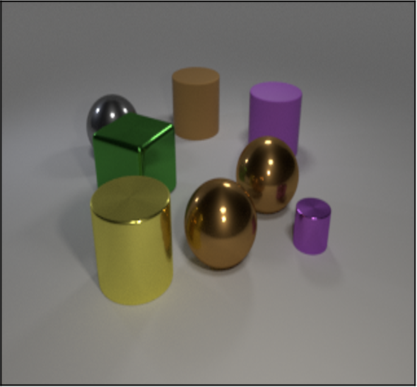
Description 2: There are two large brown spheres, a shiny yellow cylinder, a large green cube, a shiny gray sphere, a brown matte cylinder and two purple cylinders.
Description 3: There are two spheres of brown color, a cylinder of yellow color, a cube of green color, a shiny sphere of gray color, a brown cylinder of matte texture and two cylinders of purple color.

(b) Dependency graph for description 1

(c) Dependency graph for description 2

(d) Dependency graph for description 3

Figure 1: A 3D scene and three of the many possible ways to describe the scene in natural language textual description (Figure 1(a)). Figure 1(d), 1(d), 1(d) show the dependency graphs of each of the description shown in 1(a) (generated using Chen and Manning (2014)). As we can see, each graph is different from each other and needs different conditions to get information about the objects. Hence, we will need a large number of graphs with their associated rules to map all possible descriptions and it is not practically feasible.

Researchers have been trying to improve text-to-scene generation for a long time. The concept of scene generation from natural language description was first introduced by Adorni and Di Manzo (1983). Coyne and Sproat (2001) developed a system that takes a text description and renders a scene. However, their generated scene may not always be coherent. Later, many approaches have utilized machine learning techniques to generate 3D indoor scene Chang et al. (2014, 2015, 2017) and infer interaction with objects Balint et al. (2015); Krishnaswamy and Pustejovsky (2016) from text. They convert the input description into a dependency graph Chen and Manning (2014) and extract the object information in a deterministic way. For example, each description shown in figure 1(a) will be mapped to different dependency graphs (figure 1(d), 1(d), 1(d)) and will need different conditions to extract the information. Hence, the users need to provide their input in a predefined structure, otherwise the input can not be processed. A pragmatic solution should be able to process free-form text descriptions so that the users can provide their input without any constraint. It may utilize advanced deep learning techniques to design a solution for this problem as these techniques have been proved efficient to capture free-form input contexts in related fields Medhat et al. (2014); Lai et al. (2018).

Figure 2: Our proposed two-stage pipeline for text-to-scene generation. 1) The input scene description is passed through a neural architecture and the information about each object is extracted. 2) The information is passed through a renderer (made with Blender Blender (2020)) and the final scene is generated by grounding to an abstract layout, choosing 3D models to instantiate and arrange.

In this paper, we aim to design a deep learning based pipeline that can generate both static and animated scenes from free-form text descriptions. For this particular study, we focus on a potential subspace of 3D scene - containing primitive shapes (cube, cylinder and sphere) and their features (color, shape, texture, motion and size). We want to understand the performance and behavior of the architecture chosen on this synthetic problem space, so that we can build upon our knowledge and understand how to approach the more generic problems. We develop a new dataset (Integrated Static and Animated Scene Generation, IScene) for this specific purpose by synthetically generating corresponding descriptions of the scenes belonging to the widely used dataset CLEVR Johnson et al. (2017). IScene contains 13,00,000 static and 14,00,000 animated scene descriptions. Our pipeline works in two stages as shown in Figure 2. We adopt an encoder-decoder architecture to extract necessary information from scene description and use a renderer (i.e, software that performs rendering) to render the corresponding scene based on the extracted information. As the encoder, we choose one of the most recent language models, TransformerXL Dai et al. (2019). For the decoder, we design a new multi-head decoder that is capable of creating the abstract layout of the corresponding scene, where each head of this decoder predicts one of the object-specific features. Here, abstract layout represents a structured description containing the specific features of each object present in the scene and the layout is then rendered into a scene. By enabling the prediction of multiple features simultaneously, our multi-head decoder is playing an important role in our overall architecture to understand various types of user inputs without the need of any deterministic condition.

We conduct empirical analysis of how our model captures the natural language contexts and generates both static and animated scenes efficiently. We also demonstrate the ability of our approach to adapt new (unseen) 3D models during inference.

Specifically, our contributions in this work are as follows -

• We design a new two-stage pipeline that can generate static as well as animated 3D scene from free-form text descriptions. In the first stage, we extract the information using a deep learning based encoder-decoder architecture. In the second stage, we render the final scene using the extracted information.

• We design a new multi-head decoder that can extract multiple object specific features to capture the scene context efficiently. To the best of our knowledge, such a multi-head decoder has not been used before for this particular task. Our new decoder plays an important role in our overall architecture to understand various types of user input. We achieve up to 98.427% accuracy on test dataset.

• We generate a new dataset - Integrated Static and Animated Scene Generation (IScene). IScene is generated programmatically under a physics-based render engine which can be extended and scaled easily. The total unique scene descriptions in this dataset are 13,00,000 and 14,00,000 for static and animated scenes, respectively. The dataset, the code for dataset generation as well as our pipeline, and the pre-trained models are available at: https://github.com/oaishi/3DScene_from_text.

2 Related Work

In this section, we discuss relevant previous works.

2.1 3D scene synthesis from text description

The concept of scene generation from natural language description was first introduced in 1983 Adorni and Di Manzo (1983). Wordseye Coyne and Sproat (2001) first implemented a pipeline which used natural description to render a static scene. However, their generated scene may not always be coherent. Their input text description needs to follow a certain pattern; otherwise the rendered scene might not be consistent and meaningful. Seversky and Yin (2006) designed a system which allows users to generate the final scene in an interactive manner from input voice and text description, where user can choose the input scene objects. Chang et al. (2014, 2015) maps the input text description into a dependency graph Chen and Manning (2014) and learns spatial knowledge. The dependency graph is used to find out relative positioning of the scene objects. Chang et al. (2017) allows to edit the scene and view from a specific position using natural language description and given input scene. Savva et al. (2016); Zhao et al. (2016) learns interaction with daily life objects from real-world examples and generates these interactions from given input description. Similarly, Krishnaswamy and Pustejovsky (2016); Balint et al. (2015) generates animated scenes on a corpus of a limited amount of motions and objects. Ma et al. (2018) can edit an input scene as per text instruction. They learn pair and group-wise positioning and existence of scene objects for coherence.

2.2 3D scene synthesis from Layout

Merrell et al. (2011); Fisher et al. (2012) learns relative positioning from a scene database layout and synthesizes a set of plausible new scene layouts from a given input scene. Fisher et al. (2015) provides functional plausibility of an arrangement of objects from an input 3D scan using an activity model learned from an annotated 3D scene and model database. Zhou et al. (2019) proposes a neural message-passing approach to complete a given incomplete 3D scene and predict object type at a specific query location. Wang et al. (2019) generates completes floor graph with object instances and positioning from input empty or incomplete graph. The graph is further used to instantiate a 3D scene by iterative insertion of 3D models. Zhang et al. (2020) presents a framework for indoor scene synthesis, while given a room geometry and a list of objects with learnt priors. Chen et al. (2020) proposes a novel 3D-house generation architecture. Their system takes linguistic description as input and uses Graph Convolutional Network to predict the room layout. Their system also includes a generative adversarial network module which generates floor textures of each room. The textures and layout are passed to the renderer to generate the final 3D house layout.

2.3 Image and video generation from text description

Over last decade, many studies proposed novel generative models for generating image from text description using Generative Adversarial Network (GAN) Goodfellow et al. (2014) and Variational Autoencoder Kingma and Welling (2013). Zhang et al. (2017); Xu et al. (2018); Reed et al. (2016); Chen et al. (2018); Yan et al. (2016); Mansimov et al. (2015); Li et al. (2019a) propose various kinds of novel architecture for generating images from text. Johnson et al. (2018) generate images from scene graph. Some recent studies are focusing on image generation from text in an iterative manner where one or two actors engage in giving instruction about the scene El-Nouby et al. (2019); Kim et al. (2017); Cheng et al. (2018); Benmalek et al. (2018); Tan et al. (2019); Sharma et al. (2018). Li et al. (2019b) generates a series of images which form a story altogether. A related study is to generate video from story plot Gupta et al. (2018). Pan et al. (2017); Li et al. (2018) generate videos from caption.

3 Objective

For our task of static and animated scenes generation from free-form text descriptions, we use the dataset CLEVR (A Diagnostic Dataset for Compositional Language and Elementary Visual Reasoning) Johnson et al. (2017), extensively used in the literature. CLEVR is generated in the Blender Engine Blender (2020), using random combinations of primitives (Sphere, Cube and Cylinder) and object-features (color, shape, size and texture). CLEVR also provides Compositional Generalization Test (CoGenT), where the dataset is divided under two conditions (conditionA, conditionB). Based on CLEVR, We generate our Integrated Static and Animated Scene Generation (IScene) dataset (See Section 4 for details).

We work on CLEVR for multiple reasons. First, the object types, object features, location and camera position of each associated scene used in CLEVR are publicly available. Hence, we can use this information as ground truth to validate our approach. Second, CLEVR uses question template for visual reasoning. These question templates use the ground truth information for generating different types of questions. Similarly, we can design description template for generating different types of descriptions. Third, each object has a minimum four associated features that provide a wide range of possible combinations and possible scene descriptions.

(a) An example static scene with
corresponding description of each category

(b) An example animated scene with corresponding narrative description

Figure 3: Examples from IScene Dataset

We will validate our approach from the following perspectives:

1. Ability of our approach with similar data patterns: We will test our trained model on a similar combination of object features seen during training (referred to as conditionA/condA in CLEVR). The result will show how our pipeline captures known data patterns. We will use non-overlapping data points to train, test and validate our model.

2. Ability of our approach with novel data patterns: We want to test how our model performs on a novel combination of object features during inference (referred to as conditionB/condB in CLEVR). For example, any data points including red cube is not present in the training set. During inference, we will test our model on data points containing red cube. The result will show how our model adapts to new data patterns.

3. Editability of our approach: We plan to test if our pipeline can provide control over edit operation. We will provide separate 3D models of the same scene objects to our renderer script and analyze if these are executed correctly.

For each of the aforementioned validation task, we consider both static and animated 3D scenes.

4 IScene dataset

(a) Distribution of texture

(b) Distribution of size

(c) Distribution of shape

(d) Distribution of motion

(e) Distribution of color

(f) Randomly discarded object-feature
in scene description

(g) Distribution of description per category

Figure 4: Different Distribution of our Dataset

In this section, we describe in details the data generation process of our integrated Static and Animated Scene Generation (IScene) dataset. We also show the analysis of our data distribution.

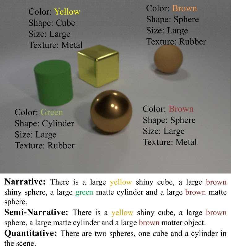
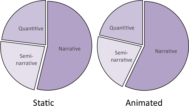
Our pipeline will take text descriptions as input and generate the corresponding 3D scenes. Hence, each data point in our dataset will comprise natural language scene description and corresponding attributes of the 3D scene. Under the current scope of our work, we consider three description families: Narrative, Semi-Narrative and Quantitative for our free-form text description. A narrative description contains a detailed description of the scene. Here, information about each feature of each object type is mentioned explicitly. In figure 3(a), we can see each object-feature of the cube (color: yellow, size: large, texture: metal) is mentioned the narrative description. In practical cases, very detailed information of a scene might not always be available. To allow our pipeline perform with limited description, we consider semi-narrative descriptions. A semi-narrative description includes a subset of randomly chosen features of each object in a scene. In figure 3(a), we can see that the size of the cube is not mentioned in the semi-narrative description. A quantitative description is a high-level abstraction of a scene where only the number of objects present in the scene are included. In figure 3(a), we can see that there are two spheres present in the scene and corresponding quantitative description. We use templates to generate the corresponding descriptions based on the ground truth information. These description templates can be extended further to generate even more types of descriptions.

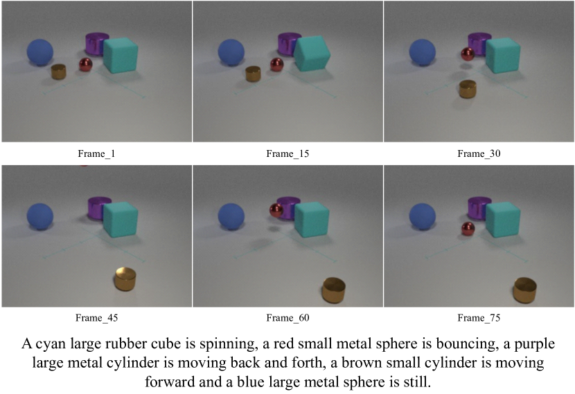
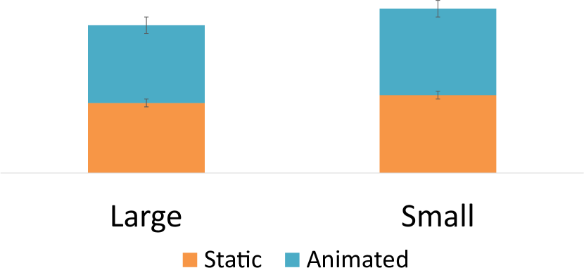
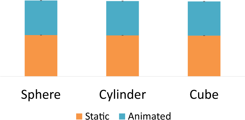
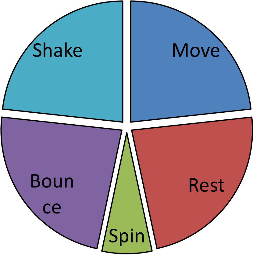
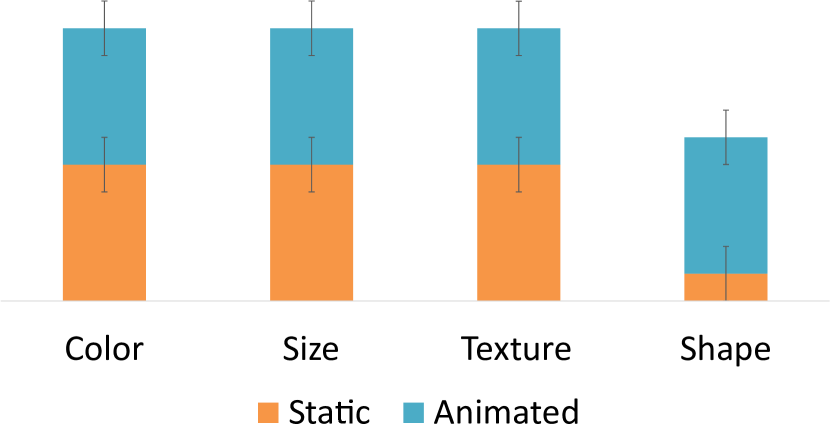
For an animated scene, we enhance ground truth information from CLEVR by inducing motion following Girdhar and Ramanan (2020). Under the current scope of our work, we consider five simple atomic motions - Spin, Bounce, Shake, Move and Rest. We assign a motion with each scene object randomly. The effect of Rest and Spin are seemingly the same for cylinder and sphere, hence we do not consider Spin for these two shapes in our data preparation. Figure 4(d) reports the distribution of the five motions in our dataset. Apart from Spin, the distribution of the remaining four motions are even. Due to the restriction over the motion Spin, it’s occurrence is lower than the others. We generate motions as program templates which can be further extended to include a new variety of motions. The recorded animations are three seconds long by default. However, it can be tuned as well. The scene description for animated scenes is generated similarly to the static scenes under three families as described above. An example animated scene from our dataset with the corresponding narrative description is shown in Figure 3(b).

Description Family	Static Scene Description	Animated Scene Description
Narrative	Train: 4,90,000 condA: 1,05,000 condB: 1,05,000	Train: 5,60,000 condA: 1,20,000 condB: 1,20,000
Semi-Narrative	Train: 2,10,000 condA: 45,000 condB: 45,000	Train: 2,10,000 condA: 45,000 condB: 45,000
Quantitative	Train: 2,10,000 condA: 45,000 condB: 45,000	Train: 2,10,000 condA: 45,000 condB: 45,000
Total	13,00,000	14,00,000

Table 1: Total count of our dataset

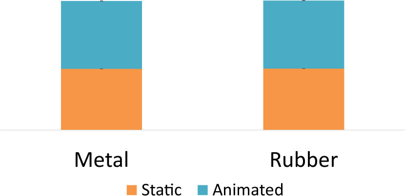
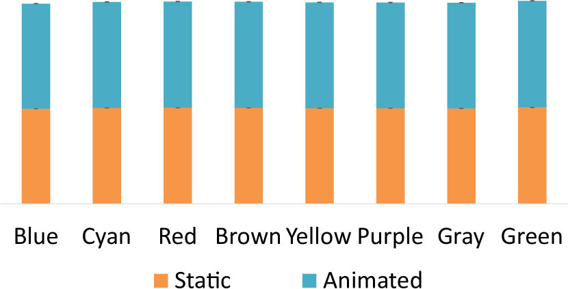
There are multiple options and degrees of complicacy to describe a scene. For preparing our standard train-test-validation set, we prepare 13 and 14 description templates for static and animated scenes, respectively that are further diversified by using synonyms. To divide our dataset in train-test-validation splits, we use the same data splits used in CLEVR, as it is an established benchmark. The total count of our dataset is shown in Table 1. The distribution of each description family for static and animated scenes are shown in Figure 4(g). We also provide some more details on our IScene dataset. Figure 4(e), 4(a), 4(b), 4(c) reports the distribution of color, texture, size and shape, respectively. The distribution of each of these object-features in both static and animated scenes are even. Figure 4(f) reports the distribution of missing object-feature information in semi-narrative and qualitative description. It is worth mentioning that all plausible biases are carefully discarded by weighted loss calculation during training the model (see Section 5.4 for details).

5 Our Pipeline

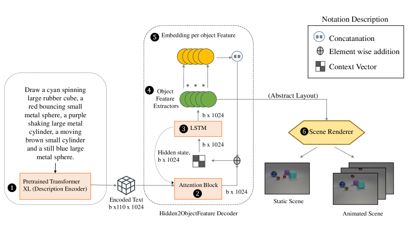
In this section, we describe different components of our pipeline. Our pipeline has three major components: Description Encoder (Section 5.1), Hidden2ObjectFeature Decoder (Section 5.2) and Scene Renderer (Section 5.6). Figure 5 shows the overall architecture of our pipeline.

Figure 5: The overall pipeline of our methodology being applied on a sample text description to generate the corresponding scene. (1) Text is encoded by TransformerXL (description encoder). (2) Attention is applied on the encoded text (from 1) and the previous hidden state of the LSTM (from 3). (3) LSTM takes as input the context vector (addition of the outputs from 5 and 2). (4) Object feature extractor generates the abstract layout of the scene and passes to 6. (5) Embedding per object feature embeds and concats the output from 4 and passes to 3. (6) Scene renderer generates the static or animated scenes from the abstract layout as specified by the user.

5.1 Description Encoder

To encode our scene description into a deep contextual vector, we use one of state-of-the-art architectures, TransformerXL Dai et al. (2019). We use the pretrained model of TransformerXL from HuggingFace Distribution Wolf et al. (2019). Transformers are proven to work well to capture the context and encode the information in a meaningful vector space. The motivation of including TransformerXL is to allow our pipeline capture the usefulness under low-resource constraints. The encoding is done according to the following equation:

$$H_{0}=E(T_{d})$$ (1)

Where $T_{d}$ is the scene description containing $d$ words, $H_{0}$ $\in$ $\mathbb{R}^{d\times 1024}$ represents the encoded hidden vectors for all the input words and $E(.)$ is the pretrained TransformerXL model (as encoder).

5.2 Hidden2ObjectFeature Decoder

We design a new multi-head decoder (referred as Hidden2ObjectFeature) which maps the encoded vector to object-feature distribution. Our decoder is specially architected to extract multiple object-features parallely and is capable to decode descriptions from different description families efficiently.

We use single-layer uni-directional LSTM Hochreiter and Schmidhuber (1997) as our base decoder unit. We apply attention Bahdanau et al. (2014) on the encoded hidden vectors (Section 5.1), $H_{0}$ and previous hidden state, $h_{t-1}$. Attention mechanism allows us the understand and capture the corresponding portions of input description which are more important while generating a specific output token. For example, intuitively, the words ”a cyan spinning large rubber cube” are most important while generating the cube as output in Figure 5. We will further analyze the output of our attention layer in Section 7.

After applying attention on $H_{0}$ and $h_{t-1}$, we get the context vector, $\hat{c}_{t}$. The addition of $\hat{c}_{t}$ and input, $i_{t}$ - is passed through the LSTM layer. Specifically,

$$a_{t}=tanh(W_{1}H_{0}+W_{2}h_{t-1}+b_{1})$$ (2)

$$\hat{a}_{t}=softmax(W_{3}a_{t}+b_{2})$$ (3)

$$\hat{c}_{t}=\hat{a}_{t}H_{0}$$ (4)

$$y_{t},h_{t}=LSTM(\hat{c}_{t}+i_{t},h_{t-1})$$ (5)

Here $W_{n},b_{n}$, and $h_{n}$ specify weight matrices, biases, and hidden vectors, respectively. $\hat{a}_{t}$ is the attention distribution over input vectors $H_{0}$ for generating the output $y_{t}$ as time-step $t$. The input $i_{t}$ is generated by the $N$ embedding layers of the decoder in the previous time step $t-1$ (to be elaborated later in Section 5.3)

The output, $y_{t}$ from LSTM is expected to be representing one object in the scene. $y_{t}$ is passed through $N$ separate dense layers to generate $N$ object-features, where $N$ is the number of object-features (depicted as Object Feature Extractors in Figure 5). The motivation is to predict each object-feature separately, because they are mutually independent. As we are using multiple dense layers parallely, our decoder is multi-headed in nature.

Let $f_{t}=[f_{t,1},f_{t,2},\dots,f_{t,N}]$ be $N$ object-features generated from $y_{t}$. Then, each $f_{t,i}~{}\in~{}f_{t}$ can be calculated using the Equation 6.

$$f_{t,i}=softmax(W_{f_{i}}~{}y_{t}+b_{f_{i}})$$ (6)

Here, $W_{f_{i}}$ and $b_{f_{i}}$ are the weight and bias of the dense layer that generates the $i-th$ object-feature $f_{t,i}$.

5.3 Multi-head Decoder-Embedding

To further ensure equal emphasis of each object-feature, the input for the next state is obtained from the object-features of the current state. For each of the object-features, there is one unique embedding layer $\epsilon_{i}(.)$, generating the object-feature-embedding vector $emb_{t,i}$ according to Equation 7.

$$emb_{t,i}=\epsilon_{i}(f_{t,i})$$ (7)

The embedding vectors $[emb_{t,1},emb_{t,2},\dots,emb_{t,N}]$ are concatenated to generate the input vector $i_{t+1}$, which is then summed with the context vector generated by the attention mechanism (as shown in Equation 5).

5.4 Loss Function

Intuitively, each object-feature plays equal role for a successful scene generation. Hence, we calculate weighted negative log likelihood loss for each object-feature. The weighting in considered to nullify any bias in the dataset.

For calculating the loss, the rescaling weight given to each class is calculated according to the distribution of object-features of our dataset. This distribution is depicted in Figure 4.

5.5 Object-Feature Accuracy Metric

As each object-feature is equally important for a successful scene generation, during evaluation we check if each object-feature, $f_{i}^{j}$ of each object matches with the ground truth information, $t_{i}^{j}$. Hence, the Object-Feature Accuracy, $acc$, can be derived using Equation 8 and 9.

$$acc=\frac{1}{l*n}\sum\limits_{i=1}^{l}\sum\limits_{j=1}^{n}a_{i}^{j}$$ (8)

$$a_{i}^{j}=\begin{cases}0&\text{if $f_{i}^{j}\neq t_{i}^{j}$}\\ 1&\text{otherwise}\end{cases}$$ (9)

Here, $l$ refer to the number of objects in the scene and $n$ is the number of object-features for each of the objects.

5.6 Scene Renderer

To render the final 3D scene from the abstract layout output of decoder, we prepare a Blender scene renderer script. Our script takes the layout and perform all necessary post-processing which includes camera setup, light positioning, 3D model loading and animation setup.

6 Experiment

In this section, we discuss our experimental setup (Section 6.1), evaluation metrics (Section 6.2), and hyperparameter settings (Section 6.3).

6.1 Experimental Setup

To the best of our knowledge, there has not been any prior study on static and animated 3D scene generation from free-form text descriptions. Hence, We evaluate and compare between three variations of our proposed model. Our first model, $M_{static}$ is trained on static scene descriptions. The second model, $M_{animated}$ is trained on animated scene descriptions. The third and final model is an oracle model, $M_{full}$ that is trained on both static and animated scene descriptions. We prepare a separate training, validation and test set for each model. The overview of the data count used for each model configuration is used in Table 2. It is worth mentioning, each set of training, validation and test dataset contains non-overlapping data points selected from the whole dataset (Table 1).

Model	Train	Validation	Test
$M_{static}$	1,00,000	condA: 5000 condB: 5000	condA: 6400 condA : 6400
$M_{animated}$	1,00,000	condA: 5000 condB: 5000	condA: 6400 condB: 6400
$M_{full}$	s: 50,000 a: 50,000	condA: 2500(s) + 2500(a) condB: 2500(s) + 2500(a)	condA: 3200(s) + 3200(a) condB: 3200(s) + 3200(a)

Table 2: Train-Validation-Test Split (s and a denote static and animated description respectively)

6.2 Evaluation Metric

We evaluate our pipeline on the following metrics.

6.2.1 Object-Feature Accuracy

As discussed in Section 5.5, we evaluate if each object-feature is the same as the ground truth object-feature information. Object-feature accuracy will show how accurately our model (Section 5) can understand the natural language description.

6.2.2 Structural Similarity Index (SSIM)

Structural Similarity Index Wang et al. (2004) is a standard metric for predicting the perceived quality of images and videos Li et al. (2019b). After the final scene is rendered (Section 5.6), we use SSIM to compare the generated image (static scene) and video (animated scene) with the ground truth. The result will show how accurately our pipeline can generate scenes with respect to ground truth as well as understand the natural language description.

6.3 Hyperparameter Settings

We did an extensive search over the possible space of hyperparameters using the validation set (discussed in Section 6.1) to select learning rate (0.0001 to 0.1), dropout rate (0 to 0.8), LSTM hidden dimension (128 to 2048), teacher forcing ratio (0% to 80%). The best set of hyperparameters is mentioned below which we use throughout our final experiments:

• Learning Rate = $0.01$

• Dropout Rate = $0.1$

• Teacher Forcing Ratio = $50\%$

• LSTM Input Dimension = Dimension of the Context vector, $\hat{c}_{t}$ (discussed in Section 5, Equation 5) = $1024$

• LSTM Hidden Dimension = Dimension of Final Dense Layer Input, $y_{t}$ (discussed in Section 5, Equation 6) = $1024$

We ran all the experiments and analyses with a batch size of 520 on the same machine with Intel core i7-7700 CPU (4 cores), 16GB RAM, NVIDIA GeForce GTX 1070 GPU (8GB memory). During training, all our models reach convergence within 120 epochs and take approximately 78 hours.

7 Result and Discussion

In this section, We present the results obtained by our models. We also provide several analysis over the generated scenes and model performance.

We train each of our models for 120 epochs until convergence with a validation step after every 10 epochs. As Figure 6 reports, the expected performance stabilizes and the error decreases significantly after 120 epochs. At this point, we report our final accuracy over the metrics discussed in Table 3 in Section 6.2. Here we show evaluation on both known and novel combinations of object feature (referred as ConditionA and ConditionB in section 3 respectively). We show some of the generated static and animated scenes during testing in Figure 7 and 9 respectively.

Model	ConditionA (Known combination)		ConditionB (Novel combination)
	Object Feature Accuracy	SSIM	Object Feature Accuracy	SSIM
$M_{static}$	98.427	0.801	94.270	0.809
$M_{animated}$	97.482	0.906	93.234	0.857
$M_{full}$	94.910	static: 0.812 animated: 0.849	90.040	static: 0.813 animated: 0.888

Table 3: Accuracy and SSIM of our models on test set

Figure 6: The expected validation performance for $M_{static},~{}M_{animated},~{}M_{full}$ Dodge et al. (2019)

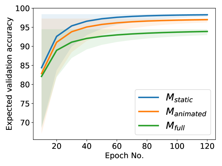
The results show that our pipeline performs consistently for all of $M_{static},~{}M_{animated},~{}M_{full}$. The slight decrease in object-feature accuracy of $M_{animated}$ from $M_{static}$ is due to the inclusion of motion which enforces the model to learn one extra object-feature (motion) than $M_{static}$. Similarly, the decrease in object-feature accuracy of $M_{full}$ is due to the extra constraints over the model. However, we see that the relative difference between these configurations is negligible. This proves the effectiveness of our proposed pipeline for both static and animated scenes. The accuracy also shows that the model performs almost similarly on joint (both static and animated scene using the same model) generation and disjoint (only static or animated scene using a single model) generation. This proves the robustness of our architecture to generate static as well animated scenes using the same configuration.

(a) Description: Draw a large yellow colored cylinder of matte texture, a large cyan colored cube of matte texture, a large brown colored cylinder of shiny texture, a large red colored cube of matte texture and a large brown colored cylinder of shiny texture.

(b) Description: Draw a small brown matte object, a small cyan matte object, a large matte cylinder, a large yellow shiny object, a small matte sphere, a small gray cylinder, a blue shiny cylinder, a large shiny cylinder, a gray matte cylinder and a large yellow shiny object.

(c) Description: There are four spheres and one cylinder.

Figure 7: Few examples of generated static scene using our pipeline with corresponding input descriptions.

Figure 8: Attention map for a successful test sample generated by our pipeline. Scene description and predicted outputs are shown on X and Y axes, respectively.

(a) Description: Draw a green metal small sphere, a purple metal large cylinder, a red rubber small sphere, a gray metal small sphere, a blue rubber large cube, a cyan rubber large cylinder, a gray metal large cube and a blue rubber small sphere.

(b) Description: A rocking cyan matte sphere, a small rocking gray matte object, a small rocking shiny cylinder, a large rocking blue matte object, a spinning blue matte cube, a small moving brown sphere and a rocking blue shiny cube. (One of the objects is occluded in the figure)

(c) Description: There are a yellow moving metal large sphere, a cyan still metal small cylinder, a yellow moving metal small cube, a green moving metal small cylinder, a blue rocking metal large cube and a brown bouncing rubber large sphere.

Figure 9: Few examples of generated animated scene using our pipeline with corresponding input descriptions.

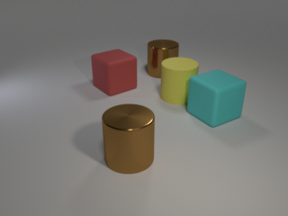
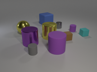
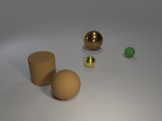
The performance of each model on known and novel combination is also noteworthy. The small margin of accuracy between these combinations shows our pipeline has a very small bias on data pattern and works efficiently for novel description as well. Overall, the higher accuracy strengthens the applicability of our system for text-to-scene generation.

7.1 Case Study

In this section, we analyze two particular outputs from our test set  generated by our pipeline as shown in Figure 10.

Figure 10: Case Study using two successful example of generated and ground truth static scene with corresponding narrative description (left) & generated and ground truth animated scene with corresponding semi-narrative description (right) during inference.

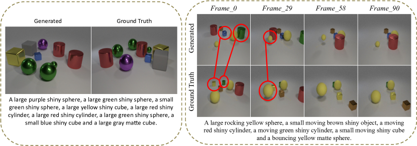
On the left, we can see the generated and ground truth static scenes with corresponding narrative scene description. Here we observe that every feature of an object, i.e., color, shape, size, and texture matches with the ground truth for all nine scene objects.

On the right, we can see the generated and ground truth animated scenes with corresponding semi-narrative scene description. As we can see, every motion of all the six objects matches with the ground truth and input description. However, ‘a small moving shiny cube’ has been mapped to a ‘a small blue moving shiny cube’ whereas ground truth scene is ‘a small yellow moving shiny cube’. Our pipeline successfully maps the texture, shape, and size mentioned for this object. As the color of the cube was not mentioned in the input, it was impossible to infer the ground truth information, and hence the generated animated scene could not reflect it.

7.2 Result Analysis

In this section, We analyze if our model captures the scene context from description correctly. For this, we focus on the output of the attention layer discussed in Section 5.2. Figure 8 shows the attention map of a successful test example during inference. As the value gets closer to 1 and as the color goes closer to white, it depicts that the word is given more importance (higher attention weight) by our model. As expected, cube, red, color, shiny are more important while generating the first object (i.e., ‘cube’). Similarly, we can see that the words cylinder and sphere are more important while generating the second and third objects, i. e., ‘cylinder’ and ‘sphere’, respectively.

Figure 11: The same description is being mapped to two different models of sphere without hampering the performance. Our pipeline thus allows us to use different 3D models even during inference

7.3 Editability

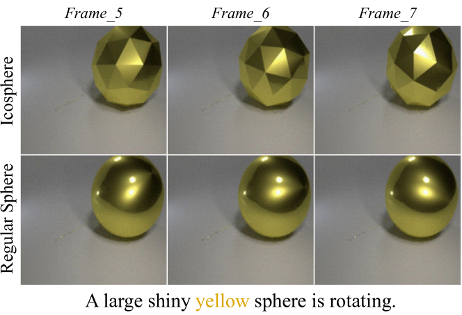
In practical life, we will often find the need of new or modified 3D models. For example, each movie has a unique set of characters. Hence, we want our system to be able to work on different variations of 3D models. Hence, we show the editability of our pipeline which will enable our system to process novel models unseen at training time. Figure 11 reports a successful datapoint in inference. Although the descriptions of both the scenes are the same, the first scene includes an icosphere which represents a sphere in low-poly graphics. The second scene includes the regular smooth sphere used in the literature. Thus, using the same description and same training parameters, our pipeline allows us to control and change the settings, models, and features if needed.

8 Conclusion and Future Work

In this work, we have built a pipeline that generates static as well as animated 3D scenes from different free-form scene descriptions. For our experiment, we have prepared a large synthetic dataset which consists of 13,00,000 and 14,00,000 unique static and animated scene descriptions, respectively. We achieve upto 98.427% accuracy on test dataset in detecting the 3D objects features successfully. We also showed how our pipeline can adapt to new and unseen 3D models at the test phase. We believe that our approach would assist greatly in 3D production.

In future, we wish to further extend our dataset for accommodating more complex scene descriptions and explore advanced Graph Networks. We also wish to explore the applicability of our system in the context of real-world. A possible application can arise immediately in children education. It can help children in learning basic mathematics using visual component. For example, if we generate one scene with four spheres and another scene with two spheres - we can teach them that there are two spheres less in the second scene than the first one. Similarly, we can use our system to teach children in other subjects besides mathematics.

References

- Adorni and Di Manzo (1983) Giovanni Adorni and Mauro Di Manzo. 1983. Natural language input for scene generation. In First Conference of the European Chapter of the Association for Computational Linguistics.
- Bahdanau et al. (2014) Dzmitry Bahdanau, Kyunghyun Cho, and Yoshua Bengio. 2014. Neural machine translation by jointly learning to align and translate. arXiv preprint arXiv:1409.0473.
- Balint et al. (2015) John Balint, Jan M Allbeck, and Michael R Hieb. 2015. Automated simulation creation from military operations documents. In Interservice/Industry Training, Simulation and Education Conference, volume 15227. I/ITSEC Orlando, Florida.
- Benmalek et al. (2018) Ryan Y. Benmalek, Claire Cardie, Serge Belongie, Xiadong He, and Jianfeng Gao. 2018. The neural painter: Multi-turn image generation.
- Blender (2020) Blender. 2020. Blender script. Most areas of Blender can be scripted, including animation, rendering, import and export, object creation and automating repetitive tasks (Accessed on 05/16/2020).
- Chang et al. (2015) Angel Chang, Will Monroe, Manolis Savva, Christopher Potts, and Christopher D. Manning. 2015. Text to 3D scene generation with rich lexical grounding. In Proceedings of the 53rd Annual Meeting of the Association for Computational Linguistics and the 7th International Joint Conference on Natural Language Processing (Volume 1: Long Papers), pages 53–62, Beijing, China. Association for Computational Linguistics.
- Chang et al. (2014) Angel Chang, Manolis Savva, and Christopher D Manning. 2014. Learning spatial knowledge for text to 3d scene generation. In Proceedings of the 2014 Conference on Empirical Methods in Natural Language Processing (EMNLP), pages 2028–2038.
- Chang et al. (2017) Angel X Chang, Mihail Eric, Manolis Savva, and Christopher D Manning. 2017. Sceneseer: 3d scene design with natural language. arXiv preprint arXiv:1703.00050.
- Chen and Manning (2014) Danqi Chen and Christopher D Manning. 2014. A fast and accurate dependency parser using neural networks. In Proceedings of the 2014 conference on empirical methods in natural language processing (EMNLP), pages 740–750.
- Chen et al. (2018) Kevin Chen, Christopher B Choy, Manolis Savva, Angel X Chang, Thomas Funkhouser, and Silvio Savarese. 2018. Text2shape: Generating shapes from natural language by learning joint embeddings. arXiv preprint arXiv:1803.08495.
- Chen et al. (2020) Qi Chen, Qi Wu, Rui Tang, Yuhan Wang, Shuai Wang, and Mingkui Tan. 2020. Intelligent home 3d: Automatic 3d-house design from linguistic descriptions only. In Proceedings of the IEEE/CVF Conference on Computer Vision and Pattern Recognition, pages 12625–12634.
- Cheng et al. (2018) Yu Cheng, Zhe Gan, Yitong Li, Jingjing Liu, and Jianfeng Gao. 2018. Sequential attention gan for interactive image editing via dialogue.
- Coyne and Sproat (2001) Bob Coyne and Richard Sproat. 2001. Wordseye: an automatic text-to-scene conversion system. In Proceedings of the 28th annual conference on Computer graphics and interactive techniques, pages 487–496.
- Dai et al. (2019) Zihang Dai, Zhilin Yang, Yiming Yang, Jaime Carbonell, Quoc V. Le, and Ruslan Salakhutdinov. 2019. Transformer-xl: Attentive language models beyond a fixed-length context.
- Dodge et al. (2019) Jesse Dodge, Suchin Gururangan, Dallas Card, Roy Schwartz, and Noah A. Smith. 2019. Show your work: Improved reporting of experimental results. In Proceedings of EMNLP.
- El-Nouby et al. (2019) Alaaeldin El-Nouby, Shikhar Sharma, Hannes Schulz, Devon Hjelm, Layla El Asri, Samira Ebrahimi Kahou, Yoshua Bengio, and Graham Taylor. 2019. Tell, draw, and repeat: Generating and modifying images based on continual linguistic instruction. In The IEEE International Conference on Computer Vision (ICCV).
- Fisher et al. (2012) Matthew Fisher, Daniel Ritchie, Manolis Savva, Thomas Funkhouser, and Pat Hanrahan. 2012. Example-based synthesis of 3d object arrangements. ACM Transactions on Graphics (TOG), 31(6):1–11.
- Fisher et al. (2015) Matthew Fisher, Manolis Savva, Yangyan Li, Pat Hanrahan, and Matthias Nießner. 2015. Activity-centric scene synthesis for functional 3d scene modeling. ACM Transactions on Graphics (TOG), 34(6):1–13.
- Girdhar and Ramanan (2020) Rohit Girdhar and Deva Ramanan. 2020. CATER: A diagnostic dataset for Compositional Actions and TEmporal Reasoning. In ICLR.
- Goodfellow et al. (2014) Ian Goodfellow, Jean Pouget-Abadie, Mehdi Mirza, Bing Xu, David Warde-Farley, Sherjil Ozair, Aaron Courville, and Yoshua Bengio. 2014. Generative adversarial nets. In Z. Ghahramani, M. Welling, C. Cortes, N. D. Lawrence, and K. Q. Weinberger, editors, Advances in Neural Information Processing Systems 27, pages 2672–2680. Curran Associates, Inc.
- Gupta et al. (2018) Tanmay Gupta, Dustin Schwenk, Ali Farhadi, Derek Hoiem, and Aniruddha Kembhavi. 2018. Imagine this! scripts to compositions to videos. In Proceedings of the European Conference on Computer Vision (ECCV), pages 598–613.
- Heath (2020) Nick Heath. 2020. What is artificial general intelligence? Verything you need to know about the path to creating an AI as smart as a human. (Accessed on 23/10/2020).
- Hochreiter and Schmidhuber (1997) Sepp Hochreiter and Jürgen Schmidhuber. 1997. Long short-term memory. Neural computation, 9(8):1735–1780.
- Johnson et al. (2018) Justin Johnson, Agrim Gupta, and Li Fei-Fei. 2018. Image generation from scene graphs. pages 1219–1228.
- Johnson et al. (2017) Justin Johnson, Bharath Hariharan, Laurens van der Maaten, Li Fei-Fei, C. Lawrence Zitnick, and Ross Girshick. 2017. Clevr: A diagnostic dataset for compositional language and elementary visual reasoning. In The IEEE Conference on Computer Vision and Pattern Recognition (CVPR).
- Kim et al. (2017) Jin-Hwa Kim, Nikita Kitaev, Xinlei Chen, Marcus Rohrbach, Byoung-Tak Zhang, Yuandong Tian, Dhruv Batra, and Devi Parikh. 2017. Codraw: Collaborative drawing as a testbed for grounded goal-driven communication. arXiv preprint arXiv:1712.05558.
- Kingma and Welling (2013) Diederik P Kingma and Max Welling. 2013. Auto-encoding variational bayes.
- Krishnaswamy and Pustejovsky (2016) Nikhil Krishnaswamy and James Pustejovsky. 2016. Voxsim: A visual platform for modeling motion language. In Proceedings of COLING 2016, the 26th International Conference on Computational Linguistics: System Demonstrations, pages 54–58.
- Lai et al. (2018) Tuan Manh Lai, Trung Bui, and Sheng Li. 2018. A review on deep learning techniques applied to answer selection. In Proceedings of the 27th International Conference on Computational Linguistics, pages 2132–2144, Santa Fe, New Mexico, USA. Association for Computational Linguistics.
- Li et al. (2019a) Bowen Li, Xiaojuan Qi, Thomas Lukasiewicz, and Philip H. S. Torr. 2019a. Controllable text-to-image generation. In NeurIPS.
- Li et al. (2019b) Yitong Li, Zhe Gan, Yelong Shen, Jingjing Liu, Yu Cheng, Yuexin Wu, Lawrence Carin, David Carlson, and Jianfeng Gao. 2019b. Storygan: A sequential conditional gan for story visualization. In Proceedings of the IEEE Conference on Computer Vision and Pattern Recognition, pages 6329–6338.
- Li et al. (2018) Yitong Li, Martin Renqiang Min, Dinghan Shen, David Carlson, and Lawrence Carin. 2018. Video generation from text. In Thirty-Second AAAI Conference on Artificial Intelligence.
- Ma et al. (2018) Rui Ma, Akshay Gadi Patil, Matthew Fisher, Manyi Li, Sören Pirk, Binh-Son Hua, Sai-Kit Yeung, Xin Tong, Leonidas Guibas, and Hao Zhang. 2018. Language-driven synthesis of 3d scenes from scene databases. ACM Transactions on Graphics (TOG), 37(6):1–16.
- Mansimov et al. (2015) Elman Mansimov, Emilio Parisotto, Jimmy Ba, and Ruslan Salakhutdinov. 2015. Generating images from captions with attention. CoRR, abs/1511.02793.
- Medhat et al. (2014) Walaa Medhat, Ahmed Hassan, and Hoda Korashy. 2014. Sentiment analysis algorithms and applications: A survey. Ain Shams engineering journal, 5(4):1093–1113.
- Merrell et al. (2011) Paul Merrell, Eric Schkufza, Zeyang Li, Maneesh Agrawala, and Vladlen Koltun. 2011. Interactive furniture layout using interior design guidelines. ACM transactions on graphics (TOG), 30(4):1–10.
- Pan et al. (2017) Yingwei Pan, Zhaofan Qiu, Ting Yao, Houqiang Li, and Tao Mei. 2017. To create what you tell: Generating videos from captions. In Proceedings of the 25th ACM international conference on Multimedia, pages 1789–1798.
- Reed et al. (2016) Scott Reed, Zeynep Akata, Xinchen Yan, Lajanugen Logeswaran, Bernt Schiele, and Honglak Lee. 2016. Generative adversarial text to image synthesis. arXiv preprint arXiv:1605.05396.
- Savva et al. (2016) Manolis Savva, Angel X Chang, Pat Hanrahan, Matthew Fisher, and Matthias Nießner. 2016. Pigraphs: learning interaction snapshots from observations. ACM Transactions on Graphics (TOG), 35(4):1–12.
- Seversky and Yin (2006) Lee M Seversky and Lijun Yin. 2006. Real-time automatic 3d scene generation from natural language voice and text descriptions. In Proceedings of the 14th ACM international conference on Multimedia, pages 61–64.
- Sharma et al. (2018) Shikhar Sharma, Dendi Suhubdy, Vincent Michalski, Samira Ebrahimi Kahou, and Yoshua Bengio. 2018. Chatpainter: Improving text to image generation using dialogue. ArXiv, abs/1802.08216.
- Tan et al. (2019) Fuwen Tan, Song Feng, and Vicente Ordonez. 2019. Text2scene: Generating compositional scenes from textual descriptions. In Proceedings of the IEEE Conference on Computer Vision and Pattern Recognition, pages 6710–6719.
- Wang et al. (2019) Kai Wang, Yu-An Lin, Ben Weissmann, Manolis Savva, Angel X Chang, and Daniel Ritchie. 2019. Planit: Planning and instantiating indoor scenes with relation graph and spatial prior networks. ACM Transactions on Graphics (TOG), 38(4):1–15.
- Wang et al. (2004) Zhou Wang, Alan C Bovik, Hamid R Sheikh, and Eero P Simoncelli. 2004. Image quality assessment: from error visibility to structural similarity. IEEE transactions on image processing, 13(4):600–612.
- Wolf et al. (2019) Thomas Wolf, Lysandre Debut, Victor Sanh, Julien Chaumond, Clement Delangue, Anthony Moi, Pierric Cistac, Tim Rault, Rémi Louf, Morgan Funtowicz, et al. 2019. Transformers: State-of-the-art natural language processing. arXiv preprint arXiv:1910.03771.
- Xu et al. (2018) Tao Xu, Pengchuan Zhang, Qiuyuan Huang, Han Zhang, Zhe Gan, Xiaolei Huang, and Xiaodong He. 2018. Attngan: Fine-grained text to image generation with attentional generative adversarial networks. pages 1316–1324.
- Yan et al. (2016) Xinchen Yan, Jimei Yang, Kihyuk Sohn, and Honglak Lee. 2016. Attribute2image: Conditional image generation from visual attributes. In European Conference on Computer Vision, pages 776–791. Springer.
- Zhang et al. (2017) Han Zhang, Tao Xu, Hongsheng Li, Shaoting Zhang, Xiaogang Wang, Xiaolei Huang, and Dimitris N Metaxas. 2017. Stackgan: Text to photo-realistic image synthesis with stacked generative adversarial networks. In Proceedings of the IEEE international conference on computer vision, pages 5907–5915.
- Zhang et al. (2020) Song-Hai Zhang, Shao-Kui Zhang, Wei-Yu Xie, Cheng-Yang Luo, and Hong-Bo Fu. 2020. Fast 3d indoor scene synthesis with discrete and exact layout pattern extraction. arXiv preprint arXiv:2002.00328.
- Zhao et al. (2016) Xi Zhao, Ruizhen Hu, Paul Guerrero, Niloy Mitra, and Taku Komura. 2016. Relationship templates for creating scene variations. ACM Transactions on Graphics (TOG), 35(6):1–13.
- Zhou et al. (2019) Yang Zhou, Zachary While, and Evangelos Kalogerakis. 2019. Scenegraphnet: Neural message passing for 3d indoor scene augmentation. In Proceedings of the IEEE International Conference on Computer Vision, pages 7384–7392.