Subgrid-scale energy transfer and associated coherent structures in turbulent flow over a forest-like canopy

Abstract

Large eddy simulation allows to incorporate the important driving physics of turbulent flow through forest- or vegetation-like canopies. In this paper we investigate the effects of vortex stretching and coherent structures on the subgrid-scale (SGS) turbulence kinetic energy (TKE). We present three simulations (SGS-d/s/w) of turbulence-canopy interactions. SGS-d assumes a local, dynamic balance of SGS production with SGS dissipation. SGS-s averages the SGS contributions of coherent structures over Lagrangian pathlines. SGS-w assumes that an average cascade of TKE from large- to small-scales occurs through the process of vortex stretching. We compare the consequences of considering a forest of the same morphology as immersed solids or an immersed canopy. Our results show clear differences in the characteristics of flow and turbulence, while both the cases exhibit canopy mixing layers. The results also show that the consideration of vortex stretching resolves about $18$% more TKE with respect to classical Deardorff’s TKE model. These observations indicate that the aerodynamic response of the forest canopy is linked to the morphology of the forest cover. Sweep- and ejection-events of the spatially intermittent coherent structures in forests as well as their role in transporting momentum, energy, and scalars are discussed.

1 Introduction

In the atmospheric boundary layer (ABL), the aggregate effect of a large collection of vertical obstacles (e.g., trees, buildings, etc) Brunet94 ; Stvredova2012 ; Philips2013 ; Park2015 ; Miri2017 is to squeeze the turbulence-containing surface layer between the outer layer and the canopy-roughness sublayer Shaw92 ; Finnigan2000 ; Finnigan2009 . For example, the Earth Observatory Report of NASA indicates the hight ($h$) of forests can be up to $70$ m. The roughness effect of such a forest may influence a height $3h$ to $5h$ from the ground Belcher2012 . During the past three decades, the turbulence kinetic energy (TKE) budget of such canopies was thoroughly scrutinized by wind-tunnel and large-eddy simulation (LES). Past work suggest that the pressure transport is dominant in the lowest two-third ($2h/3$) of forest canopies Brunet94 ; Finnigan2000 ; Marjoribanks2016 ; however, large-scale coherent structures are primarily responsible for the turbulent transfer between forests and the atmosphere Shaw92 ; Raupach96 ; Dupont2009 ; Finnigan2009 ; Konstantin2018 . A substantial work also focused on parameterizing the aggregate effects of the form drag induced by the canopies. There are few important questions associated with the transition of length scales of coherent structures, such as how to realistically represent the unresolved part of the turbulent transport in the canopy-roughness sublayer, where the energy-containing motions are inherently under-resolved by LES.

In this article we follow the vorticity transport theory of Taylor Taylor32 in which subgrid scale turbulence is regarded as an effect of vortex stretching rather than as a diffusion of straining motion. The local differences in pressure would affect the momentum of an eddy, and thus, the strain rate provides incorrect rate of turbulence dissipation, thereby requiring ad-hoc modification of SGS models for ABL flows. Based on the vortex stretching hypothesis, we present LES results for a turbulent flow over forest-like canopies in ABL. Vortex stretching appears as an appealing candidate for SGS modeling because the direction of maximal stretching is the direction of maximum positive eigenvalues of the strain tensor. In other words the stretching of vortices sets the rate of dissipation through the enstrophy production. The consideration of vortex stretching can be useful for canopy flows because in the surface layer, the energy-containing length-scale diminishes, and anisotropy strengthens. The most widely used SGS models for ABL flows Moeng2015 needs dynamic adjustments of model parameters in order to capture the TKE budget and the local backscatter of energy. In LES (e.g. Deardorff70 ; Deardorff73 ; Deardorff74 ; Deardorff80 ), vortex stretching could be directly linked to the energy containing resolved modes of the solution of Navier-Stokes equations. Recent work on LES of canopy flows indicate that vortex stretching and coherent structures can be useful for advancing subgrid models Shaw92 ; Finnigan2000 ; Dupont2008 ; Dupont2009 ; Finnigan2009 ; Yan2017 ; Konstantin2018 . Some investigations (e.g. Finnigan2000 ; Finnigan2009 ; Dupont2009 ) have emphasized that the morphology of the canopy usually leads to considerable scatter of the SGS coherent motion in the roughness sublayer, which is dominated by the stretching of small-scale vortices.

In LES, the turbulence eddy-viscosity

$$\nu_{\hbox{\tiny sgs}}=(C_{s}\Delta_{\hbox{\tiny LES}})^{2}(2\mathcal{S}_{ij}\mathcal{S}_{ij})^{1/2}$$ (1)

was proposed by Smagorinsky smagorinsky , which ensures that $-\mathcal{S}_{ij}\tau_{ij}+C_{\epsilon}k^{3/2}_{\hbox{\tiny sgs}}/\Delta_{\hbox{\tiny LES}}=0$; i.e. the dissipation $-C_{\epsilon}k^{3/2}_{\hbox{\tiny sgs}}/\Delta_{\hbox{\tiny LES}}$ accounts for the local production $-\mathcal{S}_{ij}\tau_{ij}$ if $\tau_{ij}-(3/2)k_{\hbox{\tiny sgs}}\delta_{ij}=2C_{k}\Delta_{\hbox{\tiny LES}}k^{1/2}_{\hbox{\tiny sgs}}\mathcal{S}_{ij}$ and $C_{s}^{2}=C_{k}^{3/2}/C_{\epsilon}$ (see Moeng2015 ). Here, $\tau_{ij}$ and $\mathcal{S}_{ij}$ are subgrid-scale stress and resolved strain, respectively. Deardorff Deardorff70 considered a local dynamic balance of the energy flux $-\tau_{ij}\mathcal{S}_{ij}$ that is to be transferred from the resolved scale motion and dissipated by the unresolved motion. This approach solves a transport equation in order to provide the eddy viscosity $\nu_{\hbox{\tiny sgs}}=C_{s}\Delta_{\hbox{\tiny LES}}k^{1/2}_{\hbox{\tiny sgs}}$ Deardorff70 . Meneveau et. al. Meneveau96 proposed to dynamically calculate $C_{s}$ by averaging the Lagrangian history of coherent structures, which is very useful when the grid is not sufficient to resolve the canopy-roughness sublayer. Sullivan et al Sullivan94 and Leveque Leveque2007 proposed to locally adjust $\nu_{\hbox{\tiny sgs}}$ by considering the fluctuating strain rates in Eq (1) instead of the resolved one. Instead of considering the rate of strain $\mathcal{S}_{ij}$, Nicoud Nicoud99 considered the trace-less symmetric part of the square of the velocity gradient tensor for estimating $\nu_{\hbox{\tiny sgs}}$. In canopy flows, it is important to consider that the energy cascade from large to small scales depends on two different mechanisms, namely, a linear transfer that accounts for the mean rate of strain $\mathcal{S}_{ij}$ in a statistical sense and a nonlinear transfer that accounts for the transition of scales of coherent structures. The guideline for such a consideration in the present study of canopy flows is a continuation of the work of Sullivan94 , Nicoud99 , and Leveque2007 .

In what follows, we begin by a general outline of canopy layer, porous media, and turbulence modeling in Sec 2. We then consider a brief comparison of the result of proposed LES with the wind-tunnel measurements in Sec 3, before highlighting the potential differences in dynamic modeling of SGS turbulence in Sec 4.

2 Materials and methods

2.1 Aerodynamic response to forest morphology and theory of porous media

The method of volume average is applied to the Navier-Stokes equation (NSE) to model the fluid dynamic response to solid obstacles as a drag force $f_{i}$ that accounts for the pressure and the viscous stress Finnigan2000 ; Finnigan2009 . If a box-filter is applied to NSE, we have the sub-filter scale kinematic stress $\tau_{ij}=\langle\tilde{u}_{i}\tilde{u}_{j}\rangle-\langle\tilde{u}_{i}\rangle\langle\tilde{u}_{j}\rangle$, where $\tilde{u}_{i}=\langle u_{i}\rangle+u^{\prime}_{i}$ is the total (filtered+subgrid) velocity in the $x_{i}$ direction. The volume averaging and the box-filtering commutes except in the canopy region. For simplicity, we may drop the symbol ‘$\langle\cdot\rangle$’ from the filtered variable, unless it is explicitly needed.

The finite volume method acts as an implicit box-filtering kernel, which separates the motion beyond the cutoff scale $\Delta_{\hbox{\tiny LES}}(\propto\sqrt[3]{\Delta x\Delta y\Delta z})$, where $(x_{1},x_{2},x_{3})=(x,y,z)$. In this study, we solve the filtered NSE for the atmospheric boundary layer flow, where the aerodynamic response to forest morphology extends from the surface $x_{3}=0$ to a height of $x_{3}=h$. The filtered equations are (where the summation convention is assumed in the rest of the article)

$$\frac{\partial{u_{i}}}{\partial{t}}+u_{j}\frac{\partial{u_{i}}}{\partial{x_{j}}}=-\frac{1}{\rho_{0}}\frac{\partial{\langle P\rangle}}{\partial{x_{i}}}-\frac{\partial p}{\partial x_{i}}-\frac{\partial{\tau_{ij}}}{\partial{x_{j}}}-f_{i},$$ (2)

$$\hbox{and }\quad\frac{\partial{u_{i}}}{\partial{x_{i}}}=0.$$ (3)

In the literature Shaw92 , a canonical framework of representing forest or vegetation canopies is to replace $f_{i}$ in the momentum equation (2) by a pressure-drag Dupont2008 . In the classical theory of porous media, $f_{i}$, in Eq (2), is expressed through the Darcy-Forchheimer model of a porous layer DeLemos2006 in which a portion of the pressure gradient of Eq (2) accounts for

$$\frac{\partial p^{\prime\prime}}{\partial x_{i}}=-\left(\frac{\nu}{K}+\frac{C_{d}|\bm{u}|}{\sqrt{K}}\right)u_{i},$$ (4)

where $p^{\prime\prime}$ is the local pressure change experienced by the canopy, $K$ is the porosity, and $C_{d}$ is a constant. It was reported in Finnigan2009 that the volume averaged pressure drag – the last term in (4) – is about three times larger than the viscous drag – the second last term in (4). The kinematic pressure-drag of a canopy is typically proportional to the product of a one-sided plant area density $\mathcal{A}\sim K^{-1/2}$ and the square of the resolved velocity Dwyer97 .

2.2 Turbulence modeling

As discussed in the introduction, turbulent motions at scales smaller than the grid spacing are accounted for through the deviatoric subgrid stress $\tau_{ij}^{\hbox{\tiny sgs}}=\tau_{ij}-(1/3)\tau_{kk}\delta_{ij}$ in the second last term of Eq (2), which is computed using the strain rate as

$$\tau_{ij}^{\hbox{\tiny sgs}}=\nu_{\hbox{\tiny sgs}}\mathcal{S}_{ij}.$$ (5)

In (5), it is assumed that the local pressure differences have no effect on the momentum transported by large eddies. Thus, the eddy viscosity $\nu_{\hbox{\tiny sgs}}$ is defined to be a product of a length scale $\Delta_{\hbox{\tiny LES}}$ and a velocity scale $\Delta_{\hbox{\tiny LES}}(2\mathcal{S}_{ij}\mathcal{S}_{ij})^{1/2}$, where the Smagorinsky-Lilly parameter $C_{s}$ determines the desired contribution of unresolved eddies or coherent structures. As the surface is approached, anisotropy in turbulence increases, and thus, the dynamic approach Germano91 of evaluating $C_{s}$ directly from the resolved field becomes important.

2.2.1 Lagrangian dynamic SGS model (SGS-s)

In the Lagrangian dynamic procedure, $C_{s}$ is determined by averaging inhomogeneous flows over a Lagrangian time scale, where one solves two additional transport equations, namely, for $\mathcal{I}_{lm}$ and $\mathcal{I}_{mm}$. Using the Germano identity $\mathcal{L}_{ij}=\mathcal{T}_{ij}-\tau_{ij}$, where the additional stress $\mathcal{T}_{ij}$ comes from the test-filtering operations at a scale $2\Delta_{\hbox{\tiny LES}}$ (or larger), the Lagrangian approach defines the model parameter $C_{s}=\sqrt{\mathcal{I}_{lm}/\mathcal{I}_{mm}}$. This approach is known to be effective for inhomogeneous flows. Yan et. al. Yan2017 observed some discrepancies in the simulation of canopy flows by the Lagrangian dynamic model, which may be attributed to the lack of appropriate test-filtering kernels because solid bodies immersed in the fluid are resolved by the work of Yan2017 . In case of considering the classical canopy model, the Lagrangian dynamic procedure can properly represent the role of subgrid-scale energy-containing motion.

2.3 Deardorff’s TKE model for canopy flows (SGS-d)

Deardorff Deardorff80 advanced the Smagorinsky-Lilly model, Eq (1), by incorporating a dynamic balance of subgrid-scale production and dissipation, where

$$\nu_{\hbox{\tiny sgs}}=C_{s}k^{1/2}_{\hbox{\tiny sgs}}\Delta_{\hbox{\tiny LES}}$$ (6)

is dynamically varied by obtaining $k_{\hbox{\tiny sgs}}^{1/2}$ from the TKE equation

$$\frac{\partial k_{\hbox{\tiny sgs}}}{\partial t}+\frac{\partial u_{j}k_{\hbox{\tiny sgs}}}{\partial x_{j}}=-\tau_{ij}\mathcal{S}_{ij}-C_{\epsilon}\frac{k^{3/2}_{\hbox{\tiny sgs}}}{\Delta_{\hbox{\tiny LES}}}+\frac{\partial}{\partial x_{j}}\left(\nu_{\hbox{\tiny sgs}}\frac{\partial k_{\hbox{\tiny sgs}}}{\partial x_{j}}\right).$$ (7)

As mentioned earlier, the Smagorinsky model Eq (1) can be derived by retaining only the first two terms in the right hand side of Eq (7). The second last term in Eq (7) can be written as $-C_{\epsilon}(\ell/\Delta_{\hbox{\tiny LES}})\epsilon_{\hbox{\tiny sgs}}$, where $\ell=k_{\hbox{\tiny sgs}}^{3/2}/\epsilon_{\hbox{\tiny sgs}}$ is the integral length scale. Notice the new parameter $C_{\epsilon}$ in Eq (7). Commonly used values of the two parameters for ABL flow simulations are $C_{s}\sim 0.1$, and $C_{\epsilon}\sim 0.93$ Moeng2015 .

In the present work, we consider the dynamic variation of the parameters $C_{s}$ and $C_{\epsilon}$, which are determined using the similar approach of classical dynamic Smagorinsky model Germano91 . Following Shaw92 we have also added a sink term in Eq (7) in order to represent the dissipation of turbulent eddies in the canopy zone Dupont2008 . Note that ref Finnigan2009 considered a constant value of $C_{s}$, where they diagnosed $k_{\hbox{\tiny sgs}}$ from the resolved flow instead of solving Eq (7). In addition to determining the velocity scale $k^{1/2}_{\hbox{\tiny sgs}}$ dynamically, the dynamic variation of $C_{s}$ and $C_{\epsilon}$ in the present study also provides useful feedback for considering such a model in turbulence resolving atmospheric boundary layer flow simulations. It is worth mentioning that the SGS-d model with constant values of the model parameters is usually considered in simulations of atmospheric boundary-layer flows Moeng84 ; Chow2019 .

2.3.1 Coherent structure-based scale-adaptive SGS model (SGS-w)

A purpose of considering coherent structures in the dynamic modeling approach (see Taylor32 ) is to address cross-scale interaction in turbulent flows by introducing scale-awareness in the eddy viscosity model Alam2015 ; Alam2018 . We have seen from the Lagrangian dynamic approach and Deardorff’s TKE-based model that it is important to adjust the velocity scale given by $k_{\hbox{\tiny sgs}}^{1/2}=\Delta_{\hbox{\tiny LES}}(2\mathcal{S}_{ij}\mathcal{S}_{ij})^{1/2}$, which improves the Smagorinsky-Lilly model (1). This is because the characteristic length scales of coherent structures varies as the flow transition from one sublayer to the other as the surface is approached. An algebraic approach of modeling the SGS TKE from the resolved velocity is to consider the scale-adaptive eddy viscosity Nicoud99 ; Nicoud2011 ; Trias2015

$$\nu_{\hbox{\tiny sgs}}=C_{w}\Delta_{\hbox{\tiny LES}}\left[\overbrace{\frac{\Delta_{\hbox{\tiny LES}}(\mathcal{S}^{d}_{ij}\mathcal{S}^{d}_{ij})^{3/2}}{(\mathcal{S}_{ij}\mathcal{S}_{ij})^{5/2}+(\mathcal{S}^{d}_{ij}\mathcal{S}^{d}_{ij})^{5/4}}}^{k_{\hbox{\tiny w}}^{1/2}}\right].$$ (8)

In Eq (8), $\mathcal{S}_{ij}^{d}$ is the trace-less symmetric part of the tensor $(\partial u_{i}/\partial x_{j})^{2}$. It can be shown that the expression with the square bracket $[\cdot]$ has an asymptotic limit of $\mathcal{O}([zu_{*}/\nu]^{3})$ as $z\rightarrow 0$, where the mean flow varies only in the wall-normal direction. Thus, in the vicinity of a solid within the viscous sublayer, $\nu_{\hbox{\tiny sgs}}$ defined by Eq (8) vanishes. We find that $\mathcal{S}_{ij}^{d}\mathcal{S}_{ij}^{d}=(2/3)Q^{2}+(1/2)|\mathcal{S}\bm{\omega}|$, where $Q$ is the second invariant of the velocity gradient tensor and $\mathcal{S}\bm{\omega}=\mathcal{S}_{ij}\bm{\omega}_{j}$ is the vortex stretching vector. In other words, if we consider the expression within $[\cdot]$ in Eq (8) for computing $k_{\hbox{\tiny sgs}}^{1/2}$, it would provide a velocity scale (i.e. the eddy viscosity) which is dynamically adjusted according to the magnitude of the coherent structure and vortex stretching. Equating the eddy-viscosity given by Eq (8) to that given by Eq (1), the constant $C_{w}$ can be determined in terms of the resolved velocity and the Smagorinsky-Lilly constant $C_{s}$. For the numerical tests reported in this paper, we have found that a constant value of $C_{w}=0.325$ provides reasonably accurate results in comparison to the two other models considered in the present study.

3 Comparison with wind-tunnel measurements

3.1 Experimental setup

A wind-tunnel model of canopy was designed with cylindrical stalks of diameter $0.00025$ m and length $0.05$ m Brunet94 . The stalks were arranged on a uniform square grid of side $0.005$ m. Briefly, the working section of the wind tunnel was $11$ [m] long, $1.8$ [m] wide, and $0.65$ [m] high. The entering flow was tripped by a fence and was passed over a $3$ m section of rough surface formed by road gravel to let the boundary layer developed before the flow had encountered the $5.15$ [m] long section of canopy. The leaf area index (LAI) of the model canopy is $0.47$. In other words, the wind-tunnel experiment represents a neutrally-stratified ABL flow over a homogeneous plant canopy in which the domain is $110h\times 38h\times 17h$. The estimated mean aerodynamic canopy height was $h=0.047$ m Brunet94 . Given the mean velocity $U_{h}=2.88$ m/s at $z=h$, the Reynolds number $\mathcal{R}e=U_{h}h/\nu$ has a value of $9.0\times 10^{3}$ in this wind-tunnel study.

3.2 Numerical setup

In the present LES, we simulate a turbulent flow over a canopy of height $h=50$ [m] which is about $1\,000$ times larger than that of the wind-tunnel study mentioned above. The computational domain $1\,440\times 720\times 500$ [m³] or $28.8h\times 14.4h\times 10h$ [m³] of this study is the same as what was considered by the LES study of Finnigan2009 (e.g. run A1). The domain is discretized into $256\times 128\times 123$ cells, where the mesh is uniform in both the horizontal directions (with $\Delta x=\Delta y=5.625$ [m]). The vertical mesh is stretched from $\Delta z=1.6$ [m] to $\Delta z=5.5$ [m], which is useful in capturing the mean shear near the bottom boundary. The flow is driven with a streamwise pressure gradient that is adjusted dynamically to yield a prescribed volume averaged streamwise speed of $U_{b}$. The results with $U_{b}=4$ [m/s] yields a mean non-dimensional wind that agrees with the wind-tunnel measurements Brunet94 . The Reynolds number ($U_{b}h/\nu$) for LES is $\mathcal{R}e=1.3\times 10^{7}$, which is $1\,477$ times larger than that in the wind tunnel experiment. Thus, the wind-tunnel data can be a scaled model of the flow represented by our LES.

Since the drag coefficient $C_{d}$ decreases as $\mathcal{R}e$ increases Brunet94 , a normalized form of the canopy drag force is considered to estimate $C_{d}$ for eq (2), where $f_{i}h/U_{b}^{2}=hC_{d}\mathcal{A}|\bm{u}|u_{i}$. We have observed that $hC_{d}\mathcal{A}=0.236$ yields a mean wind profile that agrees well with the wind profile measured in the wind-tunnel Finnigan2009 . The plant area index (PAI), $h\mathcal{A}=0.5$, yields $C_{d}=0.4725$ which is about $35$% of the $C_{d}$ quoted by Brunet94 . The total simulation time for all the results is $6$ [h] unless it is mentioned otherwise. The data from the last $N$ time steps that account for a period of $3$ h are used for obtaining the average statistics, where $\bar{u}_{i}=(1/N)\sum_{k=1}^{N}u_{i}^{k}$ and $\tau_{ij}^{R}=\overline{(u_{i}-\bar{u}_{i})(u_{j}-\bar{u}_{j})}$ are the resolved mean velocity and Reynolds stresses, respectively Pope2000 .

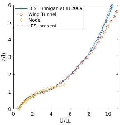
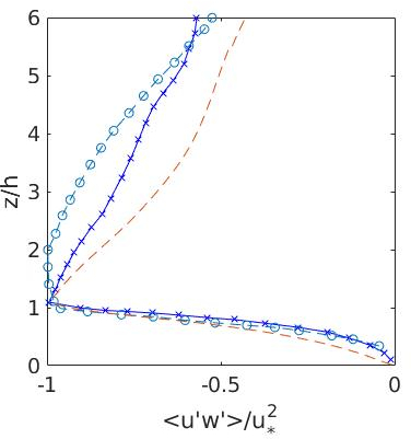
$(a)$ Mean $U(z)/u_{*}$	$(b)$ Reynolds stress $\tau^{R}_{13}/u_{*}^{2}$

Figure 1: $(a)$ The result of the present LES ($--$) is compared with wind-tunnel data ($-o-$), a reference LES ($-\times-$), and a model profile of wind speed in the canopy layer $-\diamond-$. $(b)$ Vertical profile of $\tau^{R}_{13}/u_{*}^{2}$, present LES ($--$), wind-tunnel data ($-o-$), a reference LES ($-\times-$)

3.3 Assessment of LES and wind-tunnel results

We consider wind tunnel measurements to understand the dissipation of mean energy to the production of subgrid-scale energy. The subgrid-scale energy production by the mean wind $U(z)$ is the product of $\tau^{R}_{13}=\langle u^{\prime}w^{\prime}\rangle$ and $\partial U(z)/\partial z$. One expects that $\tau_{13}^{R}$ is likely to be negative if $U(z)$ is an increasing function of $z$. In our LES, the mean streamwise velocity $\bar{u}_{1}(x,y,z)$ was averaged over the entire horizontal plane at each vertical level to obtain $U(z)=\int_{x=0}^{28.8h}\int_{y=0}^{14.4h}\bar{u}_{1}(x,y,z)dydx$. The resulting vertical profile $U(z)/u_{*}$ of the normalized streamwise velocity, which is compared with the corresponding experimental data in Fig 1$a$. The wind profile is also compared with that of the LES of Finnigan2009 . The results exhibit a good agreement among the three data sets. The deviation between results of LES and wind-tunnel data in the region of $z>h$ is primarily due to the differences in the outer boundary conditions Finnigan2009 .

A critical difference between the atmospheric boundary layer flow of over a rough surface and that over a forest comes from the roughness sublayer. In Fig 1$a$, the vertical profile of the streamwise mean wind exhibits an inflection point at $z/h=1$, while the gradient of mean wind remains positive. Below the inflection point, the wind is well approximated by $e^{-\alpha(1-z/h)}$ with $\alpha=1.60$ Brunet94 . Such exponential change of wind is a fundamental difference of canopy flow with classical rough-wall turbulent boundary layer flows. Each of the experiment and LESs has a similar wind profile in the canopy region.

In Fig 1$b$, the stress $\tau_{13}^{R}$ is normalized by the friction velocity, $u^{2}_{*}=\max\limits_{0\leq z\leq 10h}(-\tau_{13}^{R})$. Clearly, the vertical distribution of $\tau_{13}^{R}$ is negative, as expected. The most important finding is that the representation of SGS TKE by Q-criterion and vortex stretching in the SGS-w model is an acceptable representation of subgrid-scale turbulence in canopy flows. The guideline of studying SGS dissipation as a function of $Q$ and $\mathcal{S}\bm{\omega}$ comes from the earlier work of Dupont2008 , and Finnigan2009 . The role of vortex stretching in the SGS energy flux was thoroughly scrutinized by the LES study of rough-wall turbulent boundary layer Chung2009 . While the study of coherent structures in canopy flows exists, to the best of our knowledge, this work is a first-time attempt in designing an SGS model for canopy flows, which is based on coherent structures.

It is worth discussing that we have not explicitly modeled the effects of wind shear. In other words, we have neither considered a damping function nor a boundary-layer specific blending of the length scale, $\Delta_{\hbox{\tiny LES}}$ (see Mason92 ). The importance of the blending of length scale in boundary-layer meteorology in the context of the non-dynamic formulation of Deardorff’s TKE model was studied by Kurowski2018 . Recent findings of Kurowski2018 also suggests for an equivalent dynamic approach, such as SGS-w model, for LES of canopy flows, which is further discussed below.

4 Analysis and Discussion

4.1 Coherent structures and subgrid-scale motion in a canopy flow.

Consider the second invariant

$$\mathcal{Q}=\frac{1}{2}\left[\left(\frac{\partial u_{i}}{\partial x_{j}}-\frac{\partial u_{j}}{\partial x_{i}}\right)^{2}-\left(\frac{\partial u_{i}}{\partial x_{j}}+\frac{\partial u_{j}}{\partial x_{i}}\right)^{2}\right]$$ (9)

of the velocity gradient tensor $\partial u_{i}/\partial x_{j}$, which can be interpreted as an indication of the local pressure changes in the Navier-Stokes equations. A fluid region of $Q>0$ indicates that the rotation rate $\mathcal{R}_{ij}=\frac{\partial u_{i}}{\partial x_{j}}-\frac{\partial u_{j}}{\partial x_{i}}$ dominates over the strain rate $\mathcal{S}_{ij}=\frac{\partial u_{i}}{\partial x_{j}}+\frac{\partial u_{j}}{\partial x_{i}}$. However, $Q>0$ does not necessarily mean that the pressure is minimum within the region. Fig 2($a,b,c$) demonstrates the isosurface of $Q=0.2U^{2}/h^{2}$ colored by the spanwise vorticity $\omega_{y}$ (i.e. $\mathcal{R}_{13}$), where the red and blue colors denote positive and negative values, respectively. Note that a canopy flow contains the vorticity of the mean ABL flow $\langle U(z),0,0\rangle$, i.e. $\mathcal{R}_{13}=\partial u/\partial z-\partial w/\partial x$ that points toward the spanwise direction, as well as the vorticity associated with turbulent fluctuations, which is usually random. The spanwise rolls are likely to deform into inclined arched or hairpin-like structures – the precise transition of which is flow-dependent Bailey2016 . For a fully developed turbulent flow through a canopy, Fig 2 shows the the coherent structures while they are simultaneously advected, stretched, and tilted. One notes that the Reynolds shear-stress can be expressed in terms of velocity fluctuations in the direction of principal rate of strain, i.e. $\tau_{13}^{R}=(1/2)[\overline{(w^{\prime}_{*})^{2}}-\overline{(u^{\prime}_{*})^{2}}]$ (see the corresponding discussion in Davidson2004 ). Here, the notation $(\cdot)^{\prime}_{*}$ indicates that the co-ordinate system is rotated along the principal axes of the strain tensor. This means that in Fig 2 the negative (clock-wise) value of $\mathcal{R}_{13}$ is due to the Reynolds stress (e.g. Fig 2$d$) associated with large fluctuations of $w^{\prime}_{*}$ in the principal axes of the strain tensor. The qualitative description of the flow structures in Fig 2 also indicates that wind inside a forest canopy is linked to the morphology of canopy elements and their aerodynamic response to airflow Miri2017 .

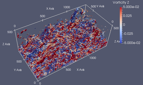
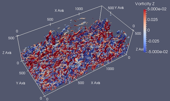
$(a)$ Q, SGS-w	$(b)$ Q, SGS-s
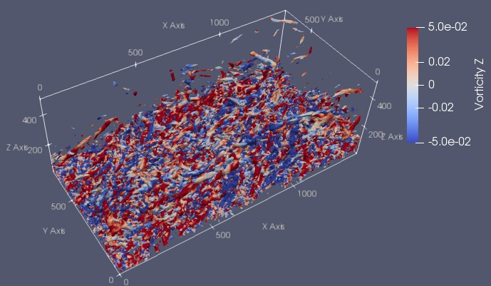
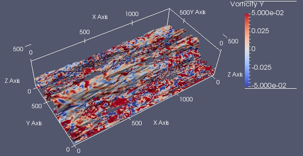
$(c)$ Q, SGS-d	$(d)$ $\tau^{R}_{13}$, SGS-w

Figure 2: A visualization of the coherent structures. Isosurfaces of the Q-criterion and the shear stress are colored by values of spanwise vorticity. $(a)$ Q-criterion, shear-adjusted SGS-w model, $(b)$ Q-criterion, dynamic Lagrangian SGS-s model $(c)$ Q-criterion, Deardorff’s TKE based SGS-d model, and $(d)$ shear-stress $\tau^{R}_{13}$, SGS-w model

4.2 Turbulence above a canopy layer

The structure of modified turbulence above the canopy layer have been studied most intensively Finnigan2009 . The mean flow kinetic energy in the canopy layer is entrained from the free atmosphere, where kinetic energy is stored. In region above the canopy layer, the modified turbulence enhances a mechanism for the vertical mixing of the mean-flow kinetic energy and the momentum. From Eq (7) we estimate that the rate of dissipation per unit mass in the layer just above the canopy is $-\overline{u^{\prime}w^{\prime}}\partial u/\partial z=u^{2}_{*}(u_{*}/\kappa z)$, where the flow is restored to the neutrally stratified turbulent atmospheric boundary layer. Therefore, the amount of dissipation within the canopy layer $z_{0}\leq z\leq z_{1}$ is given by $\int_{z_{0}}^{z_{1}}\epsilon(z)dz=(u^{3}_{*}/\kappa)\ln(z_{1}/z_{0})$. Fig 3$a$ demonstrate that two logarithmic regions exist in a fully developed turbulent flow through a canopy – one is below the tree trunk and characterized by the surface friction velocity $u_{*z_{0}}$. The other log-region is above the canopy edge, which is characterized by the canopy friction velocity is $u_{*z_{1}}$. The difference of the momentum fluxes between the two region, $u^{2}_{*z_{1}}-u^{2}_{*z_{0}}$, equals the momentum deficit caused by the canopy.

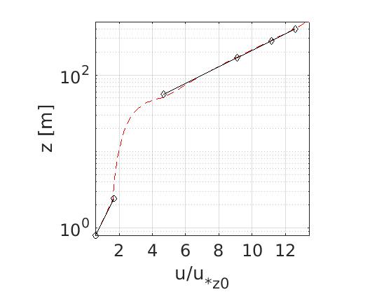
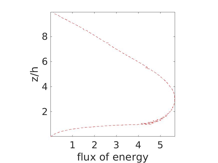
Figure 3: $(a)$ The vertical profile of mean stream-wise flow showing two logarithmic region. One is above the canopy, which is characterized by the canopy friction velocity $u_{*_{z_{1}}}$. The other is in the very bottom of the canopy, which is characterized by the surface friction velocity $u_{*_{z_{0}}}$. $(b)$ The energy flux $-\overline{u^{\prime}w^{\prime}}\partial u/\partial z$. Both plots are normalized by surface friction velocity $u_{*_{z_{0}}}$.

The statistical description of coherent structures in wall-bounded turbulent flows usually provides most of the phenomena exploited by turbulent flows over a canopy or another form of multiscale rough surfaces Adrian2007 . In that view, the coherent structures depicted in Fig 2 are responsible to carry Reynolds stresses and to transport mean momentum. To illustrate the role that Reynolds stresses would play in the production and dissipation of TKE, the vertical distribution of the TKE is presented in Fig 4. The kinematic Reynolds stress, $\tau_{ij}^{R}=-\overline{u^{\prime}_{i}u^{\prime}_{j}}$, is obtained by taking a time average of the solution during the last $3$ hours, treating this as an ensemble of large statistical samples distributed in the three-dimensional space. The TKE defined by $\tau_{ii}^{R}$ was averaged over the horizontal domain. Fig 4$a$ presents the vertical profiles of the diagonal components of the Reynolds stress, where $\sigma_{u}=\tau^{R}_{11}$, $\sigma_{v}=\tau^{R}_{22}$, and $\sigma_{w}=\tau^{R}_{33}$ are the variances of the velocity fluctuations, and half of their sum (i.e. TKE) represents turbulence intensity. The results are compared between three models, namely, SGS-w, SGS-d, and SGS-s. It is seen that the longitudinal velocity fluctuations are the largest because the shear production in a neutrally stable ABL initially feeds the energy into the $u$-component. The energy is subsequently distributed into the lateral components $v$ and $w$. As discussed earlier, the results of LES are expected to be relatively insensitive to the choice of the three SGS models if a majority of TKE is resolved. We see that each model predicts an overall expected behavior of the Reynolds stress. A variation of $18$% in the prediction of turbulence intensity with respect to SGS-w and SGS-d suggest that the TKE carried by coherent structures are captured more directly by Eq (8) than Eq (7). In the Lagrangian dynamic model, the time history of energy-carrying eddies are employed for adjusting the dissipation dynamically. A comparison of the result of locally-adaptive model (SGS-w) in Fig 4$a$ with that of Lagrangian dynamic model (SGS-s) in Fig 4$c$ also suggests that the consideration of $Q$ and $\mathcal{S}\bm{\omega}$ in the derivation of Eq (8) help to capture the dynamical role of coherent structures without solving additional transport equations.

In Fig 5, a brief sensitivity study of the model parameter $C_{w}$ of the SGS-w model is shown. Here, $C_{w}$ was estimated analytically by equating the eddy-viscosity given by Eq (8) with the eddy-viscosity of Smagorinsky-Lilly model (1), which leads to $C_{w}^{2}=C_{s}^{2}\Delta_{\hbox{\tiny LES}}\sqrt{2\mathcal{S}_{ij}\mathcal{S}_{ij}}/k_{\hbox{\tiny w}}^{1/2}$ (where $k^{1/2}_{w}$ is the expression within $[\cdot]$ in Eq (8).) To estimate $C_{w}$, we considered a simulation of homogeneous isotropic turbulence in a periodic box using $C_{s}=0.17$. It was found that a value of $C_{w}\sim 0.5$-$0.55$ persists for many eddy-turn over time for both decaying and forced turbulence. As depicted in Fig 5, the vertical profiles of the resolved TKE for $C_{w}=0.125,\,0.325,\,0.525$ are quite similar in the canopy sublayer. Based on our observation from several other numerical tests of the same canopy flow, we find that the modeled portion of the TKE $k_{\hbox{\tiny w}}$ is dynamically adjusted as the resolved flow varies by a change of $C_{w}$. Overall, a value of $C_{w}=0.325$ seems to be appropriate for canopy flows (see Fig 5$b$).

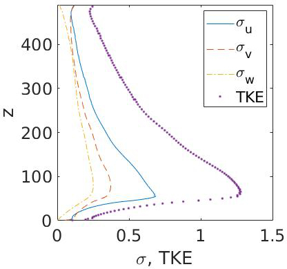
$(a)$ Scale-adaptive (SGS-w)

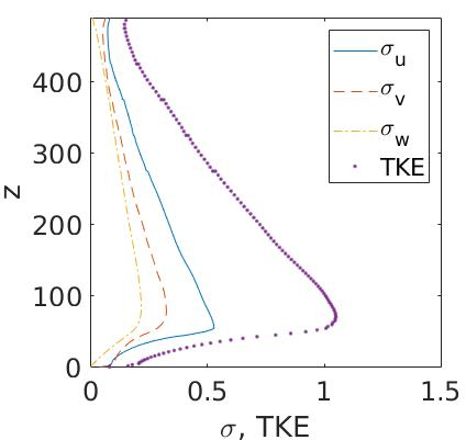
$(b)$ Deardorff’s TKE (SGS-d)

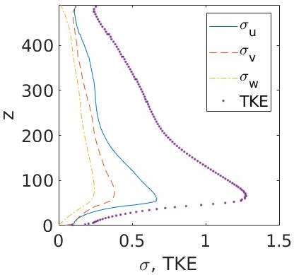
$(c)$ dynamic Lagrangian (SGS-s)

Figure 4: Vertical profiles of the Reynolds stresses, $\sigma_{u}$, $\sigma_{v}$, $\sigma_{w}$, and TKE. $(a)$ Scale-adaptive algebraic eddy-viscosity model SGS-w, which does not solve any additional transport equation; $(b)$ Deardorff’s TKE model SGS-d, which solves an additional transport equation, and $(c)$ Lagrangian dynamic model SGS-s, which solves two additional transport equations.

$(a)$

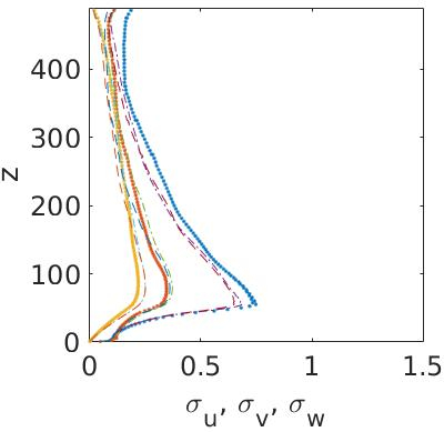
$(b)$

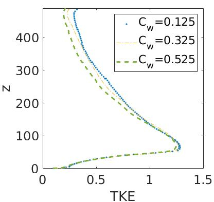
Figure 5: The result of a sensitivity study of the model parameter $C_{w}$. In $(a)$ the legend is skipped for brevity, where $\cdots$ $C_{w}=0.125$, $-\cdot-$ $C_{w}=0.325$, and $--$ $C_{w}=0.525$.

4.3 Quadrant analysis

$(a)$	$(b)$
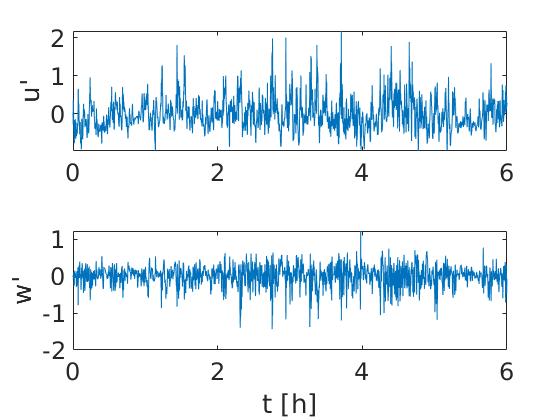
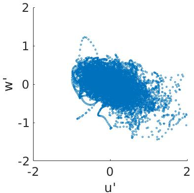
$(c)$	$(d)$
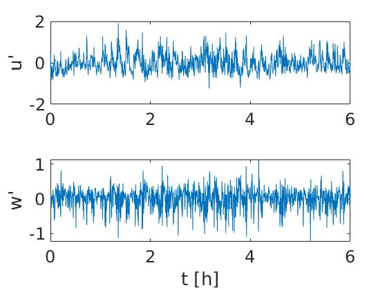
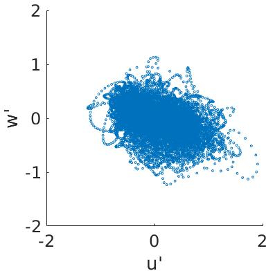
$(e)$	$(f)$

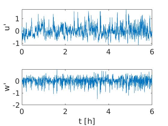
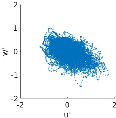
Figure 6: Time series of fluctuations in the streamwise ($u^{\prime}$) and vertical ($w^{\prime}$) velocities. Left column: time series plots of $u^{\prime}$ and $w^{\prime}$ vs $t$; right column: scattered plot of $u^{\prime}$ vs $w^{\prime}$. $(a,b)$ wall-adaptive SGS-w model, $(c,d)$ Deardorff’s TKE model, SGS-d, and $(e,f)$ dynamic Lagrangian SGS-w model

While a flow visualization technique can identify coherent structures, the quadrant analysis technique is a powerful yet simple method, to investigate the contributions of the coherent motions. The instantaneous stress $-\overline{u^{\prime}w^{\prime}}$ is viewed in the four quadrants of $u^{\prime}-w^{\prime}$ plane, namely, Q1 ($u^{\prime}>0,w^{\prime}>0$), Q2 ($u^{\prime}<0,w^{\prime}>0$), Q3 ($u^{\prime}<0,w^{\prime}<0$), and Q4 ($u^{\prime}>0,w^{\prime}<0$). In the context of ABL studies this method holds a lot of promise for a single level sonic anemometer data to determine the largest possible contributions to $-\overline{u^{\prime}w^{\prime}}$, such as statistical properties of strong “ejection-like” ($u^{\prime}<0,\,w^{\prime}>0$,  Q2) or “sweep-like” ($u^{\prime}>0,\,w^{\prime}<0$,  Q4) bursting phenomena of boundary layer turbulence. Ref Zhou99 extracted coherent structures from the DNS of a channel flow by linear stochastic estimation of “ejection-like” near-wall events. Using Haar wavelet transform, ref Watanabe2004 observed that sweep-ejection cycle has a dominant contribution to the Reynolds stress. Ref Finnigan2009 observed that the conjunction of Q2 and Q4 events produces the location of the coherent scalar microfront, and that the sweep-ejection cycle is also associated with the breaking of symmetry in flows over a vegetation canopy.

For the purpose of understanding the predictions of SGS motion by the SGS-w model, Eq (8), Fig 6 illustrates a qualitative comparison of sweep- and ejection-like events among three SGS models. The time series of the resolved SGS velocities $u^{\prime}$ (=$u-\bar{u}$) and $w^{\prime}$ (=$w-\bar{w}$) are displayed in Fig 6$(a,c,e)$, where $u$ and $w$ are resolved velocity computed at a height of $z/h=1$ on the vertical centerline of the computational domain. The nature of the time series of the velocity fluctuations with respect to three SGS models is similar, except the intermittent burst of horizontal velocity fluctuations are relatively protuberant in SGS-w/s models than the SGS-d models. This is consistent with the similarity of the flow structures depicted in Fig 4. It is evident implicitly that the rate ($\tau^{R}_{13}\mathcal{S}_{13}$) of mixing by the Reynolds stress in the forest edge – due to passing of energy from the mean flow to the turbulence – is enhanced by resolved shear $\mathcal{S}_{13}$. Fig 6$(b,d,f)$ demonstrate the scattered plots of the velocity fluctuations on the $u^{\prime}$-$w^{\prime}$ plane. Briefly, the ejection (Q2) of low-momentum are associated with the sweeps (Q4) of high momentum fluids. It is worth mentioning that an overall similarity among the plots in Fig 6$(b,d,f)$ indicates the similar nature of three dynamic modeling approaches.

5 Conclusion

In this article, a numerical study of the energy transfer between the resolved- and the subgrid-scale motions in a turbulent flow over a forest-like canopy is summarized. LES and wind-tunnel measurements of the mean vertical wind profile and the Reynolds stress suggests that the subgrid-scale energy transfer is strongly correlated with the coherent structures and vortex stretching mechanism. This result is consistent with the previous findings of Dupont2008 and Finnigan2009 .

In particular, we find that the advancement of the scale-adaptive large-eddy simulation framework is a potential methodology that correlates the SGS dissipation of TKE to the vortex stretching mechanism through the second invariant of the square of the velocity gradient tensor. Considering the form-drag experienced by a forest-like canopy in the form of three-dimensional Forchheimer stress, the wind profiles simulated by our LES agree with the corresponding profiles of wind-tunnel measurements. Incorporating the viscous drag in the form of Darcy-Forcheimer stress, this work observes two log-regions: one below the tree trunk and one above the canopy edge. The bottom log-region is characterized by the friction of the surface, and the upper log-region is characterized by the friction of the canopy with the air-flow aloft.

It is worth mentioning that this study considers three strategies of the dynamic modeling approach for canopy flows. We have analyzed scale-adaptive large-eddy simulation for canopy flows, where neither the canopy elements nor the viscous sublayer is fully resolved. The results show that capturing the effects of coherent structures captured about $18$% more SGS TKE with respect to resolving the dynamics of SGS TKE through a transport equation.

There is a substantial investigation of canopy flows, for example, see the work of Raupach96 and Finnigan2009 . However, there remains several questions in the context of SGS turbulence modeling. As nature of the canopy flow shares between mixing layer and turbulent boundary layer, it is an ideal candidate for understanding the role of self-amplification of the strain-rate with that of vortex stretching. We think that such consideration may help our future studies on understanding the transition of scales in atmospheric turbulence, particularly in ‘grey-zone’ turbulence.

References

- (1) Adrian, R.J.: Hairpin vortex organization in wall turbulence. Physics of Fluids 19(4), 041301 (2007)
- (2) Alam, J., Islam, M.R.: A multiscale eddy simulation methodology for the atmospheric ekman boundary layer. Geophysical & Astrophysical Fluid Dynamics 109(1), 1–20 (2015)
- (3) Alam, J.M., Fitzpatrick, L.P.J.: Large eddy simulation of urban boundary layer flows using a canopy stress method. Computers & Fluids 171, 65–78 (2018)
- (4) Arthur, R.S., Mirocha, J.D., Lundquist, K.A., Street, R.L.: Using a canopy model framework to improve large-eddy simulations of the neutral atmospheric boundary layer in the weather research and forecasting model. Monthly Weather Review 147(1), 31–52 (2019)
- (5) Bailey, B.N., Stoll, R.: The creation and evolution of coherent structures in plant canopy flows and their role in turbulent transport. Journal of Fluid Mechanics 789, 425–460 (2016)
- (6) Belcher, S.E., Harman, I.N., Finnigan, J.J.: The wind in the willows: Flows in forest canopies in complex terrain. Annual Review of Fluid Mechanics 44(1), 479–504 (2012)
- (7) Brunet, Y., Finnigan, J., Raupach, M.: A wind tunnel study of air flow in waving wheat: single-point velocity statistics. Boundary-Layer Meteorology 70(1-2), 95–132 (1994)
- (8) Chung, D., Pullin, D.I.: Large-eddy simulation and wall modelling of turbulent channel flow. Journal of Fluid Mechanics 631, 281–309 (2009)
- (9) Davidson, P.A.: Turbulence - An Introduction for Scientists and Engineers. Oxford University Press (2004)
- (10) De Lemos, M.: Turbulence in Porous Media: Modeling And Applications (2006)
- (11) Deardorff, J.W.: A numerical study of three-dimensional turbulent channel flow at large reynolds numbers. J. Fluid Mech. 41(2), 453–480 (1970)
- (12) Deardorff, J.W.: The use of subgrid transport equations in a three-dimensional model of atmospheric turbulence. Journal of Fluids Engineering 95, 429 (1973)
- (13) Deardorff, J.W.: Three-dimensional numerical study of the height and mean structure of a heated planetary boundary layer. Boundary-Layer Meteorology 7(1), 81–106 (1974)
- (14) Deardorff, J.W.: Stratocumulus-capped mixed layers derived from a three-dimensional model. Boundary-Layer Meteorology 18(4), 495–527 (1980)
- (15) Dupont, S., Brunet, Y.: Edge flow and canopy structure: A large-eddy simulation study. Boundary-Layer Meteorology 126(1), 51–71 (2008)
- (16) Dupont, S., Brunet, Y.: Coherent structures in canopy edge flow: a large-eddy simulation study. Journal of Fluid Mechanics 630, 93–128 (2009)
- (17) Dwyer, M.J., Patton, E.G., Shaw, R.H.: Turbulent kinetic energy budgets from a large-eddy simulation of airflow above and within a forest canopy. Boundary-Layer Meteorology 84(1), 23–43 (1997)
- (18) Finnigan, J.: Turbulence in plant canopies. Annual Review of Fluid Mechanics 32(1), 519–571 (2000)
- (19) Finnigan, J.J., Shaw, R.H., Patton, E.G.: Turbulence structure above a vegetation canopy. Journal of Fluid Mechanics 637, 387–424 (2009)
- (20) Germano, M., Piomelli, U., Moin, P., Cabot, W.H.: A dynamic subgrid scale eddy viscosity model. Physics of Fluids A 3(7), 1760–1775 (1991)
- (21) Kröniger, K., Banerjee, T., Roo, F.D., Mauder, M.: Flow adjustment inside homogeneous canopies after a leading edge – An analytical approach backed by les. Agricultural and Forest Meteorology 255, 17 – 30 (2018)
- (22) Kurowski, M.J., Teixeira, J.: A scale-adaptive turbulent kinetic energy closure for the dry convective boundary layer. Journal of the Atmospheric Sciences 75(2), 675–690 (2018)
- (23) LÉVÊQUE, E., TOSCHI, F., SHAO, L., BERTOGLIO, J.P.: Shear-improved smagorinsky model for large-eddy simulation of wall-bounded turbulent flows. Journal of Fluid Mechanics 570, 491–502 (2007)
- (24) Marjoribanks, T., Hardy, R., Lane, S., Parsons, D.: Does the canopy mixing layer model apply to highly flexible aquatic vegetation? insights from numerical modelling. Environmental Fluid Mechanics 17 (2016)
- (25) Mason, P.J., Thomson, D.J.: Stochastic backscatter in large-eddy simulations of boundary layers. Journal of Fluid Mechanics 242, 51–78 (1992)
- (26) Meneveau, C., Lund, T.S., Cabot, W.H.: A lagrangian dynamic subgrid-scale model of turbulence. Journal of Fluid Mechanics 319, 353–385 (1996). DOI 10.1017/S0022112096007379
- (27) Miri, A., Dragovich, D., Dong, Z.: Vegetation morphologic and aerodynamic characteristics reduce aeolian erosion. Scientific Reports 7(1), 12831 (2017)
- (28) Moeng, C.H.: A large-eddy-simulation model for the study of planetary boundary-layer turbulence. Journal of the Atmospheric Sciences 41(13), 2052–2062 (1984)
- (29) Moeng, C.H., Sullivan, P.: Encyclopedia of Atmospheric Sciences, 2nd Edition, vol. 4, pp. 232–240. Elsevier Ltd, Academic Press (2015)
- (30) Nicoud, F., Ducros, F.: Subgrid-scale stress modelling based on the square of the velocity gradient tensor. Flow, Turbulence and Combustion 62(3), 183–200 (1999)
- (31) Nicoud, F., Toda, H.B., Cabrit, O., Bose, S., Lee, J.: Using singular values to build a subgrid-scale model for large eddy simulations. Physics of Fluids 23(8), 085106 (2011)
- (32) Park, S.B., Baik, J.J., Han, B.S.: Large-eddy simulation of turbulent flow in a densely built-up urban area. Environmental Fluid Mechanics 15(2), 235–250 (2015)
- (33) Philips, D.A., Rossi, R., Iaccarino, G.: Large-eddy simulation of passive scalar dispersion in an urban-like canopy. Journal of Fluid Mechanics 723, 404–428 (2013)
- (34) Pope, S.B.: Turbulent Flows. Cambridge University Press (2000)
- (35) Raupach, M.R., Finnigan, J.J., Brunei, Y.: Coherent eddies and turbulence in vegetation canopies: The mixing-layer analogy. Boundary-Layer Meteorology 78(3), 351–382 (1996)
- (36) Shaw, R.H., Schumann, U.: Large-Eddy Simulation of Turbulent Flow above and within a Forest. Boundary Layer Meteorology 61, 47–64 (1992)
- (37) Smagorinsky, J.: General circulation experiments with the primitive equations. Monthly Weather Review 91, 99 (1963)
- (38) Středová, H., Podhrázská, J., Litschmann, T., Středa, T., Rožnovskỳ, J.: Aerodynamic parameters of windbreak based on its optical porosity. Contributions to Geophysics and Geodesy 42(3), 213–226 (2012)
- (39) Sullivan, P.P., McWilliams, J.C., Moeng, C.H.: A subgrid-scale model for large-eddy simulation of planetary boundary-layer flows. Boundary-Layer Meteorology 71(3), 247–276 (1994)
- (40) Taylor, G.I.: The transport of vorticity and heat through fluids in turbulent motion. Proceedings of the Royal Society of London. Series A, Containing Papers of a Mathematical and Physical Character 135(828), 685–702 (1932)
- (41) Trias, F.X., Folch, D., Gorobets, A., Oliva, A.: Building proper invariants for eddy-viscosity subgrid-scale models. Physics of Fluids 27(6), 065103 (2015)
- (42) Watanabe, T.: Large-eddy simulation of coherent turbulence structures associated with scalar ramps over plant canopies. Boundary-Layer Meteorology 112(2), 307–341 (2004)
- (43) Yan, C., Huang, W.X., Miao, S.G., Cui, G.X., Zhang, Z.S.: Large-eddy simulation of flow over a vegetation-like canopy modelled as arrays of bluff-body elements. Boundary-Layer Meteorology (2017)
- (44) Zhou, J., Adrian, R.J., Balachandar, S., Kendall, T.M.: Mechanisms for generating coherent packets of hairpin vortices in channel flow. Journal of Fluid Mechanics 387, 353–396 (1999). DOI 10.1017/S002211209900467X