Online Neural Networks for Change-Point Detection

Abstract

Moments when a time series changes its behaviour are called change points. Detection of such points is a well-known problem, which can be found in many applications: quality monitoring of industrial processes, failure detection in complex systems, health monitoring, speech recognition and video analysis. Occurrence of change point implies that the state of the system is altered and its timely detection might help to prevent unwanted consequences. In this paper, we present two online change-point detection approaches based on neural networks. These algorithms demonstrate linear computational complexity and are suitable for change-point detection in large time series. We compare them with the best known algorithms on various synthetic and real world data sets. Experiments show that the proposed methods outperform known approaches.

1 Introduction

The first works [1, 2] about change-point detection were presented in the 1950s. They utilise shifts of the mean value of signal to detect changes in the quality of the output of a continuous production process. In the following decades, a lot of other change-point detection methods were developed. They are based on different ideas and are able to recognise various changes in time series: jumps of mean and variance of a signal, correlations between its different components and other more elaborate dependencies. These algorithms are well-described in various overviews [3, 4, 5].

This study introduces two new approaches for change-point detection based on neural networks. These algorithms can be used for online detection of changes in time series behaviour. As it is shown in the following sections, they have linear computational complexity, work with multidimensional signals and are well suited for large time series. The proposed solutions are inspired by the Kullback–Leibler importance estimation procedure (KLIEP) [6], unconstrained least-squares importance fitting (uLSIF) [7, 8] and the relative uLSIF (RuLSIF) [9, 10]. These methods are used to estimate the direct probability density ratio for two samples. As demonstrated in [11], they can be used for change-point detection in time series data. Moreover, according to [4], these approaches show better results compared with other change-point detection algorithms. Their idea is based on calculation distances between pairs of observations from two different samples using RBF kernels to approximate the probability density ratio.

The first implementation of decision tree and logistic regression classifiers to analyse changes between two samples was demonstrated in [12]. However, it was not applied for change-point detection. The authors of [13] show that Convolutional Neural Networks (CNNs), trained with uLSIF loss function can be used for outlier detection in images. In recent years, several approaches based on neural networks [14, 15], with KLIEP and RuLSIF loss functions, were presented for change-point detection in time series data. It is also shown that they outperform previous methods based on RBF kernels.

2 Change-Point Detection

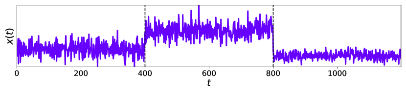
Figure 1: Example of a time series with two change-points at moments $t_{1}=400$ and $t_{2}=800$. Observations between these points have different probability distributions: $P_{1}(x(t))$ for $0<t<t_{1}$, $P_{2}(x(t))$ for $t_{1}<t<t_{2}$ and $P_{3}(x(t))$ for $t_{2}<t<1200$.

Consider a time series, where each observation for a moment $t$ is represented by a $d-$dimensional vector $x(t)\in\mathcal{R}^{d}$:

$$x(1),x(2),x(3),...,x(\tau),x(\tau+1),x(\tau+2),...$$ (1)

Assume that all observations $x(t)$ with $t<\tau$ have probability density distribution $P$, and all observations with $t\geq\tau$ are sampled from distribution $Q\neq P$. In other words, the time series changes its behaviour at moment $\tau$. Such moments are called change-points. There are may be several such points in one time series, as it is demonstrated in Fig. 1. The goal is to detect all change points with the highest quality. This is an unsupervised problem, since the true positions of change-points are not given.

Often the original time series is transformed into an autoregression form [11]:

$$X(k),X(k+1),X(k+2),...,X(\tau),X(\tau+1),X(\tau+2),...$$ (2)

where $X(t)$ is a combined vector of $k$ previous observations of the time series and is defined as:

$$X(t)=[x(t)^{T},x(t-1)^{T},...,x(t-k+1)^{T}]^{T}\in\mathcal{R}^{kd}$$ (3)

This transformation allows us to take into account time dependencies between observations and helps to improve the quality of change-point detection. It is equal to the time series in Eq. 1 with $k=1$. We also use this notation to preserve consistency with conventional notation.

3 Quality Metrics

Consider a time series with $n$ change-points at moments $\tau_{1}$, $\tau_{2}$, …, $\tau_{n}$. Suppose that an algorithm recognises $m$ change-points at moments $\hat{\tau}_{1}$, $\hat{\tau}_{2}$, …, $\hat{\tau}_{m}$. Following [5], a set of correctly detected change-points is defined as True Positive (TP):

$$\text{TP}=\{\tau_{i}|\exists\hat{\tau}_{j}:|\hat{\tau}_{j}-\tau_{i}|<M\}$$ (4)

where $M$ is a margin size and $M=50$ in our study. Then, Precision, Recall and F1-score metrics are calculated as follows:

$$\text{Precision}=\frac{|\text{TP}|}{m}$$ (5)

$$\text{Recall}=\frac{|\text{TP}|}{n}$$ (6)

$$\text{F1}=\frac{2\cdot\text{Precision}\cdot\text{Recall}}{\text{Precision}+\text{Recall}}$$ (7)

We use F1-score to measure quality of change-point detection algorithms. We also use a common measure in clustering analysis, called Rand Index (RI) [16], which is calculated in the following way. True change-points $\{\tau_{i}\}_{n}$ split the time series into $n+1$ segments $S$. Similarly, the observations are divided by the detected change-points $\{\hat{\tau}_{i}\}_{m}$ into $m+1$ segments $\hat{S}$. RI measures the similarity of these two segmentation sets. The Rand Index is then defined as

$$\text{RI}=\frac{A}{0.5~{}T(T-1)},$$ (8)

where $A$ is the number of observation pairs $x(i)$ and $x(j)$, that share the same segment, both in $S$ and $\hat{S}$; $T$ is the total number of observations in the time series and $0.5~{}T(T-1)$ gives the total number of observation pairs in the whole time series.

4 Proposed Methods

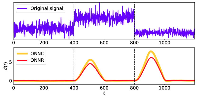
Figure 2: Example of change-point detection using the proposed algorithms. (Top) A time series with two change-points at moments $t_{1}=400$ and $t_{2}=800$. (Bottom) Change-point detection score $\bar{d}(t)$ estimated by the algorithms ONNC and ONNR.

4.1 Classification-Based Model

Consider a time series defined in Eq. (2) with several change-points. The idea of the proposed algorithm is based on a comparison of two observations $X(t-l)$ and $X(t)$ of this time series. Here $l$ is the lag size between these two observations. If there is not a change-point between them, $X(t-l)$ and $X(t)$ have the same distributions. Otherwise, they are sampled from different distributions, which means that a change-point occurred at the moment $\tau:t-l<\tau\leq t$. Repeating this comparison for all pairs of observations sequentially helps to determine the positions of all change-points in the time series.

A more general way is to compare two mini-batches of observations $\mathcal{X}(t-l)$ and $\mathcal{X}(t)$. Here, a mini-batch $\mathcal{X}(t)$, is a sequence of observations of size $n$, which is defined as:

$$\mathcal{X}(t)=\{X(t),X(t-1),...,X(t-n+1)\}$$ (9)

Further in this study, we work with these mini-batches of size $n\ll l$ in order to speed up the change-point detection algorithm.

To check whether observations in two mini-batches $\mathcal{X}(t-l)$ and $\mathcal{X}(t)$ come from the same distribution, we use a classification model based on a neural network $f(X,\theta)$ with weights $\theta$. This network is trained on the mini-batches with cross-entropy loss function $L(\mathcal{X}(t-l),\mathcal{X}(t),\theta)$,

$$L(\mathcal{X}(t-l),\mathcal{X}(t),\theta)=-\frac{1}{n}\sum_{X\in\mathcal{X}(t-l)}\log(1-f(X,\theta))-\frac{1}{n}\sum_{X\in\mathcal{X}(t)}\log f(X,\theta),$$ (10)

where all observations from $\mathcal{X}(t-l)$ are considered as the negative class and observations from $\mathcal{X}(t)$ are taken as the positive class. We use only one neural network for the whole time series and it is trained in accordance with the online learning paradigm: each pair of mini-batches is used only once and the network makes a few iterations of optimisation on each pair. Information from previous pairs are encoded in the neural network weights and each new step just slightly changes them.

The neural network $f(X,\theta)$ can be used to compare distributions of observations in the mini-batches. In this work, we use a dissimilarity score based on the Kullback-Leibler divergence, $D(\mathcal{X}(t-l),\mathcal{X}(t))$. Following [15], we define this score as

$$\begin{split}D(\mathcal{X}(t-l),\mathcal{X}(t),\theta)=&\frac{1}{n}\sum_{X\in\mathcal{X}(t-l)}\log\frac{1-f(X,\theta)}{f(X,\theta)}+\\ +&\frac{1}{n}\sum_{X\in\mathcal{X}(t)}\log\frac{f(X,\theta)}{1-f(X,\theta)}.\end{split}$$ (11)

If observations in the mini-batches are sampled from the same distribution, this dissimilarity score value is close to 0. Otherwise, it takes positive values. All steps above are combined into one algorithm called change-point detection based on Online Neural Network Classification (ONNC) and shown in Alg. 1. An example of change-point detection, using ONNC, is demonstrated in Fig. 2.

Inputs: time series $\{X(t)\}_{t=k}^{T}$; $k$ – size of a combined vector $X(t)$; $n$ – size of a mini-batch $\mathcal{X}(t)$; $l$ – lag size and $n\ll l$; $f(X,\theta)$ – a neural network with weights $\theta$;

Initialization: $t\leftarrow k+n+l$;

while $t\leq T$ do

       take mini-batches $\mathcal{X}(t-l)$ and $\mathcal{X}(t)$;

       $d(t)\leftarrow D(\mathcal{X}(t-l),\mathcal{X}(t),\theta)$;

       $\bar{d}(t)\leftarrow\bar{d}(t-n)+\frac{1}{l}(d(t)-d(t-l-n))$;

       $loss(t,\theta)\leftarrow L(\mathcal{X}(t-l),\mathcal{X}(t),\theta)$;

       $\theta\leftarrow\mathrm{Optimizer}(\mathrm{loss}(t,\theta))$;

       $t\leftarrow t+n$;

      

end while

return $\{\bar{d}(t)\}_{t=1}^{T}$ – change-point detection score

Algorithm 1 ONNC change-point detection algorithm.

4.2 Regression-Based Model

An alternative method of change-point detection is based on regression models. In this case, a regression model, based on a neural network $g(X,\theta)$, with weights $\theta$, is used to estimate the ratio between distributions of a time series observations in two mini-batches $\mathcal{X}(t-l)$ and $\mathcal{X}(t)$. Assume that all observations in $\mathcal{X}(t-l)$ have a probability density distribution $Q(X)$, and observations in $\mathcal{X}(t)$ mini-batch are sampled from the distribution $P(X)$. Then, the output of the neural network approximates the ratio between these two distributions directly

$$g(X,\theta)\approx\frac{P(X)}{Q(X)}.$$ (12)

Following the idea of the RuLSIF method [9, 10] and mathematical inference in [15], the loss function for the neural network is defined as

$$\begin{split}L(\mathcal{X}(t-l),\mathcal{X}(t),\theta)&=\frac{1-\alpha}{2n}\sum_{X\in\mathcal{X}(t-l)}g^{2}(X,\theta)+\\ &+\frac{\alpha}{2n}\sum_{X\in\mathcal{X}(t)}g^{2}(X,\theta)-\frac{1}{n}\sum_{X\in\mathcal{X}(t)}g(X,\theta),\end{split}$$ (13)

where $\alpha$ is an adjustable parameter. In this work, we take $\alpha=0.1$. Similarly to the classification-based algorithm, described in the previous section, the neural network is trained in an online learning way: all mini-batches are processed only once in time order.

While the output $g(X,\theta)$ approximates the ratio between the distributions of observations in the mini-batches, we can estimate the dissimilarity score between them using the Pearson $\chi^{2}-$divergence [15]:

$$\begin{split}D(\mathcal{X}(t-l),\mathcal{X}(t),\theta)=\frac{1}{n}\sum_{X\in\mathcal{X}(t)}g(X,\theta)-1\end{split}$$ (14)

However, the loss function and the dissimilarity score described above are asymmetric with respect to the mini-batches $\mathcal{X}(t-l)$ and $\mathcal{X}(t)$, and affect the change-point detection quality. To compensate this effect, we use two neural networks $g_{1}(X,\theta_{1})$ and $g_{2}(X,\theta_{2})$ as is described in Alg. 2. We call this algorithm change-point detection based on Online Neural Network Regression (ONNR). An example of change-point detection using this algorithm is shown in Fig. 2.

Inputs: time series $\{X(t)\}_{t=k}^{T}$; $k$ – size of a combined vector $X(t)$; $n$ – size of a mini-batch $\mathcal{X}(t)$; $l$ – lag size and $n\ll l$; $g_{1}(X,\theta_{1})$ and $g_{2}(X,\theta_{2})$ – neural network with weights $\theta_{1}$ and $\theta_{2}$ respectively;

Initialization: $t\leftarrow k+n+l$;

while $t\leq T$ do

       take mini-batches $\mathcal{X}(t-l)$ and $\mathcal{X}(t)$;

       $d_{1}(t)\leftarrow D(\mathcal{X}(t-l),\mathcal{X}(t),\theta_{1})$;

       $d_{2}(t)\leftarrow D(\mathcal{X}(t),\mathcal{X}(t-l),,\theta_{2})$;

       $d(t)\leftarrow d_{1}(t)+d_{2}(t)$;

       $\bar{d}(t)\leftarrow\bar{d}(t-n)+\frac{1}{l}(d(t)-d(t-l-n))$;

       $loss(t,\theta_{1})\leftarrow L(\mathcal{X}(t-l),\mathcal{X}(t),\theta_{1})$;

       $\theta_{1}\leftarrow\mathrm{Optimizer}_{1}(\mathrm{loss}(t,\theta_{1}))$;

       $loss(t,\theta_{2})\leftarrow L(\mathcal{X}(t),\mathcal{X}(t-l),\theta_{2})$;

       $\theta_{2}\leftarrow\mathrm{Optimizer}_{2}(\mathrm{loss}(t,\theta_{2}))$;

       $t\leftarrow t+n$;

      

end while

return $\{\bar{d}(t)\}_{t=1}^{T}$ – change-point detection score

Algorithm 2 ONNR change-point detection algorithm.

5 Data Sets

To test change-point detection algorithms, we use several synthetic and real world data sets with various numbers of dimensions. Their purpose is to estimate how different methods work in different conditions and with different kinds of change-points. The first synthetic data set is called mean jumps and contains 10 one-dimensional time series, where each observation $x(t)$ is sampled from normal distribution $x(t)\sim\mathcal{N}(\mu,\sigma)$ with mean $\mu$ and standard deviation $\sigma=1$. Change-points are generated every 200 timestamps by changing mean $\mu$ in the following way:

$$\mu_{N}=\begin{cases}0,&\mbox{if }N=1\\ \mu_{N-1}+0.2N,&\mbox{if }N=2,...,10,\end{cases}$$ (15)

where $N$ is an integer which is estimated as $200(N-1)<t\leq 200N$.

Similarly, variance jumps data set contains 10 one-dimensional time series, where each observation $x(t)$ is also sampled from normal distribution $x(t)\sim\mathcal{N}(\mu,\sigma)$ with mean $\mu=0$ and standard deviation $\sigma$. Change-points are generated every 200 timestamps by changing $\sigma$ in the following way:

$$\sigma_{N}=\begin{cases}1,&\mbox{if }N=2k+1\\ 1+0.25N,&\mbox{if }N=2k\end{cases}$$ (16)

where $N$ is an integer that is estimated as $200(N-1)<t\leq 200N$.

The last synthetic data set we use in this work is called cov jumps. It also contains 10 two-dimensional time series, where each observation $x(t)$ is sampled from multivariate normal distribution $x(t)\sim\mathcal{N}(\mu,\Sigma)$, with a vector of means $\mu=(0,0)^{T}$ and covariance matrix $\Sigma$. As previously, change-points are generated every 200 timestamps by changing $\Sigma$ in the following way:

$$\Sigma_{N}=\begin{cases}\begin{pmatrix}1&-0.1N\\ -0.1N&1\\ \end{pmatrix},&\mbox{if }N=2k+1\\ \begin{pmatrix}1&0.1N\\ 0.1N&1\\ \end{pmatrix},&\mbox{if }N=2k\end{cases}$$ (17)

where $N$ is an integer that is estimated as $200(N-1)<t\leq 200N$.

We also use two real world data sets that are publicly available and are taken from the human activity recognition domain. WISDM [17, 18] data set contains 3-dimensional signals of accelerometer and gyroscope sensors, collected from a smartphone and a smartwatch measured at a rate of 20 Hz. The signal is collected for different human activities. Their changes are considered as change-points. Each time series has 17 change-points. We use 10 samples of the smartwatch gyroscope sensors for further tests. We also downsample the signals and take only about 3000 observations per time series.

Similarly, EMG Physical Action Data Set [18] contains EMG data, which corresponds to 10 different physical activities for 4 persons. Transitions between the activities are considered as change-points. Each sample has 8 dimensions. We downsample the original signals to only about 2000 measurements per time series for the change-point detection tests.

One more interesting data set we use is called Kepler [19]. It contains data from the Kepler spacecraft that was launched in March 2009. Its mission was to search for transit-driven exoplanets, located within the habitable zones of Sun-like stars. In this work we use the one-dimensional Kepler light curves, with Data Conditioning Simple Aperture Photometry (DCSAP) data from 10 stars with exoplanets.

The next range of data sets are based on real samples for classification tasks in machine learning, collected from astronomical and high energy physics domains.

The first data set is called HTRU2 [20, 18] and describes a sample of pulsar candidates, collected during the High Time Resolution Universe Survey (South) [21]. It contains two types of astronomical objects: positive (pulsars) and negative (others), that are described by 8 features. We create 10 time series with 2000 observations $x(t)$, that are sampled from positive or negative classes with change-points at every 200 timestamps:

$$x(t)=\begin{cases}\text{random negative object},&\mbox{if }N=2k\\ \text{random positive object},&\mbox{if }N=2k+1\end{cases}$$ (18)

where $N$ is an integer that is estimated as $200(N-1)<t\leq 200N$. Changes of the object classes are considered as change-points. Then, we scale each components of the time series by reducing their mean values to 0 and variance to 1. After that, we add white noise generated from the normal distribution $\mathcal{N}(\mu=0,\sigma=2)$. The goal of this transformation is to reduce the difference between the distributions of the classes and make change-point detection more difficult.

One more astronomical data set is MAGIC Gamma Telescope Data Set [18], which describes signals registered in the Cherenkov gamma telescope, from high energy particles, that come from space. There are also two kinds of signals: positive and negative, that correspond to gamma and hadron particles respectively. Each signal is described by 10 features. Similar to the HTRU2 data set, we create 10 time series by sampling observations $x(t)$ as is shown in (19) and adding noise generated from $\mathcal{N}(\mu=0,\sigma=5)$ to each component.

SUSY [22, 18] is a data set from a high energy physics domain. It contains positive (signal) and negative (background) events, observed in a particle detector and described by 18 features. We create 10 time series in the same way as for the HTRU2 data set.

One more high energy physics data set is called Higgs [22, 18] and contains positive (signal) and negative (background) events. Each event is described by 21 features. While it is a quite difficult data set for change-point detection, we create 10 time series with 4000 observations $x(t)$, that are sampled from the positive or negative classes:

$$x(t)=\begin{cases}\text{random negative object},&\mbox{if }N=2k\\ \text{random positive object},&\mbox{if }N=2k+1\end{cases}$$ (19)

where $N$ is an integer that is estimated as $400(N-1)<t\leq 400N$. Changes of the object classes are considered as change-points.

The final data set we use in this work is MNIST [18], which contains 1794 samples of hand-written digits. Each digit is described by 64 features. We create 10 time series with 1794 observations $x(t)$ by stacking all randomly shuffled 0 digits, then adding all randomly shuffled 1 digits and repeating this for all classes. Changes of the digits are considered as change-points. Then, similarly to the HTRU2 data set, we add white noise, generated from normal distribution $\mathcal{N}(\mu=0,\sigma=5)$.

6 Experiments

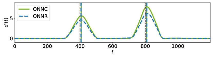
Figure 3: Change-point detection score estimated by the algorithms ONNC and ONNR after the time shift: $\bar{d}^{\prime}(t)=\bar{d}(t+l+n)$, where score $\bar{d}(t)$ is shown in Fig. 3. Positions of the score peaks are considered as positions of the detected change-points.

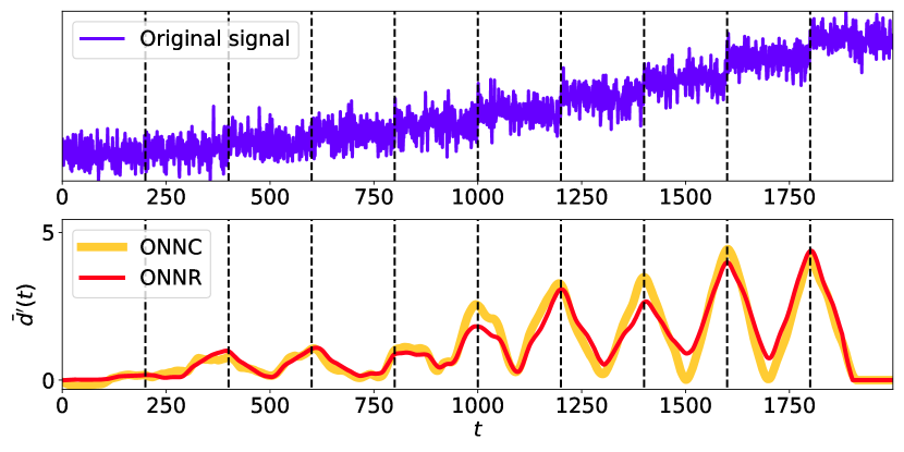
Figure 4: Example of change-point detection score $\bar{d}^{\prime}(t)$ estimated by ONNC and ONNR algorithms (bottom) for a time series in mean jumps data set (top).

We compare the proposed methods with 4 known methods for change-point detection. These methods are Binseg [23, 24], Pelt [25], Window [5] and RuLSIF [11]. There are several reviews [4, 5, 26], where it is shown that they demonstrate the best quality of change-point detection on various data sets.

Implementations of Binseg, Pelt and Window algorithms in the ruptures [5] package are used in further experiments. The Binseg and Window methods require the set up of the number of change-points needed to be found in a time series. The optimal number for each sample is estimated from a range $[1,40]$, using grid search, by maximising RI quality metric. The Window algorithm also has width hyperparameter. To provide good resolution between consecutive change points, we take $\textit{width}=20$ for Kepler, $\textit{width}=200$ for Higgs and $\textit{width}=100$ for the rest of the data sets described in Sec. 5. Similarly, the Pelt method has a hyperparameter pen for penalty. Its optimal value is found in the range $[0,10]$ using grid search with step $0.5$ by maximising the RI quality metric. For all these algorithms, we use the rbf cost function as the most universal choice which works with any kind of change-points.

The regularisation parameter, $\lambda$, and width $\sigma$ of RBF kernels in the RuLSIF algorithm are also optimised using grid search in the range $[10^{-3},10^{3}]$. For the window size hyperparameter, we take the same values as for the width hyperparameter in the Window algorithm.

For the proposed algorithms in this work, ONNC and ONNR, we use the following hyperparameters. The lag size $l=20$ for Kepler, $l=200$ for Higgs and $l=100$ for the rest of the data sets. The number of previous observations in (3) $k=1$. The mini-batch size $n=\{1,10\}$; the number of epochs of the neural network optimiser $n\_epochs=\{1,10\}$ and the learning rate $lr=\{0.1,0.01\}$. The optimal values of these hyperparameters are estimated using grid search by maximising the RI quality metric. The neural network optimiser is Adam.

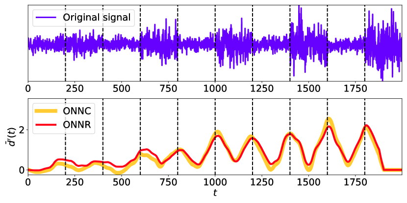
Figure 5: Example of change-point detection score $\bar{d}^{\prime}(t)$ estimated by ONNC and ONNR algorithms (bottom) for a time series in variance jumps data set (top).

Dataset	Binseg	Pelt	Window	RuLSIF	ONNC	ONNR
Mean jumps	0.99	0.99	0.98	0.98	0.98	0.99
Variance jumps	0.99	0.99	0.98	0.98	0.98	0.98
Cov jumps	0.97	0.96	0.97	0.95	0.97	0.97
MNIST	0.99	0.97	0.97	0.91	0.98	0.97
WISDM	0.99	0.99	0.99	0.99	0.99	0.99
EMG	0.97	0.97	0.97	0.97	0.98	0.98
Kepler	0.95	0.99	0.99	0.89	1.00	1.00
SUSY	0.98	0.98	0.97	0.95	0.98	0.98
Higgs	0.96	0.91	0.95	0.75	0.97	0.97
MAGIC	0.96	0.97	0.97	0.85	0.96	0.97
HTRU2	0.98	0.98	0.97	0.96	0.98	0.97

Table 1: Average values of RI quality metric for all change-point detection algorithms and data sets.

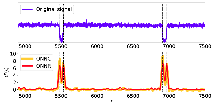
Figure 6: Example of change-point detection score $\bar{d}^{\prime}(t)$ estimated by ONNC and ONNR algorithms (bottom) for a time series in Kepler data set (top).

Binseg, Pelt, Window and RuLSIF are offline algorithms for change-point detection. This means that they process observations of a time series in any order they need. It helps to detect change-points without time delay. Our algorithms are online and process the observations sequentially in time order. This creates a time delay in the change-point detection score $\bar{d}(t)$ as it is demonstrated in Fig. 2. Assuming, that firstly, the whole time series is processed and then the quality is measured, we transform the score $\bar{d}(t)$ to the offline-equivalent form by applying time shift on the sum of the lag $l$ and mini-batch $n$ sizes: $\bar{d}^{\prime}(t)=\bar{d}(t+l+n)$ as is shown in Fig. 3. Positions of the score peaks are considered as positions of the detected change-points.

Dataset	Binseg	Pelt	Window	RuLSIF	ONNC	ONNR
Mean jumps	0.94	0.92	0.93	0.97	0.97	0.97
Variance jumps	0.92	0.95	0.90	0.97	0.97	0.96
Cov jumps	0.65	0.62	0.82	0.85	0.90	0.93
MNIST	0.97	0.92	0.89	0.79	0.96	0.97
WISDM	0.88	0.86	0.94	0.94	0.96	0.97
EMG	0.90	0.89	0.82	0.95	0.97	0.97
Kepler	0.60	0.97	0.88	0.14	1.00	0.97
SUSY	0.90	0.92	0.83	0.76	0.99	0.97
Higgs	0.51	0.18	0.52	0.23	0.76	0.76
MAGIC	0.68	0.83	0.77	0.58	0.88	0.87
HTRU2	0.91	0.90	0.82	0.85	0.98	0.93

Table 2: Average values of F1-score quality metric for all change-point detection algorithms and data sets.

Each algorithm is applied to all time series in a data set. Then, the quality metric values are averaged over all samples in it. The average values of the RI and F1-score quality metrics are presented in Tab. 1 and Tab. 2 respectively. The results show that ONNC and ONNR have similar or better RI values for all data sets and demonstrate the best values of the F1-score for all data sets, except mean jumps and MNIST, where these algorithms show the same quality as other methods. Examples of change-point detection score, estimated by ONNC and ONNR algorithms, for several time series are demonstrated in Fig. 4, 5, 6, 7 and 8.

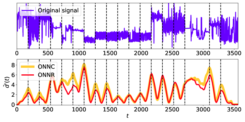
Figure 7: Example of change-point detection score $\bar{d}^{\prime}(t)$ estimated by ONNC and ONNR algorithms (bottom) for a time series in WISDM data set (top).

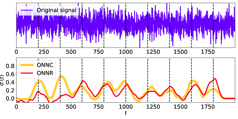
Figure 8: Example of change-point detection score $\bar{d}^{\prime}(t)$ estimated by ONNC and ONNR algorithms (bottom) for a time series in HTRU2 data set (top).

7 Discussion

In this work, two new online algorithms for change-point detection in time series data are introduced. They are based on sequential comparison of two mini-batches of observations, by neural networks, to estimate whether they have the same distribution or not. Each pair of mini-batches is processed only once, which provides good scalability of the algorithms.

The results in Tab. 1 and Tab. 2 demonstrate that the algorithms are able to detect various kinds of change-points in high-dimensional time series. Also, ONNC and ONNR methods demonstrate better quality of the detection on noisy data sets than other approaches. Reducing the noise level increases the quality for all algorithms considered here. To explain this, one can consider an RBF kernel for two observations $X(i)$ and $X(j)$ from Eq. (2):

$$K(X(i),X(j))=\exp(-\frac{d_{ij}^{2}}{2\sigma^{2}})$$ (20)

and

$$d_{ij}=\sqrt{(X_{1}(i)-X_{1}(j)^{2}+...+(X_{kd}(i)-X_{kd}(j)^{2}},$$ (21)

where $\sigma$ is the kernel width; $d_{ij}$ is the Euclidean distance between the observations. The kernels are used in the cost functions of Binseg, Pelt, Window and RulSIF methods. In these equations, all signal components are taken into account equally. Uninformative and noisy components increase the variance of the distances, which reduces the sensitivity of the cost functions and decreases the quality of change-point detection.

	Computations	Memory
Binseg	$\mathcal{O}(T^{3})$	$\mathcal{O}(T^{2})$
Pelt	$\mathcal{O}(T^{3})$	$\mathcal{O}(T^{2})$
Window	$\mathcal{O}(W^{2}T)$	$\mathcal{O}(W^{2})$
RuLSIF	$\mathcal{O}(KWT)$	$\mathcal{O}(KW)$
ONNC	$\mathcal{O}(T)$	$\mathcal{O}(l)$
ONNR	$\mathcal{O}(T)$	$\mathcal{O}(l)$

Table 3: Computational complexity and memory usage of the change-point detection algorithms. $T$ - the number of observation in a time series; $W$ is the window width; $K$ is the number of kernels; $l$ is the lag size.

As was considered previously, the ONNC and ONNR algorithms described in Alg. 1 and Alg. 2, respectively, process mini-batches of a time series observations sequentially. Thus, the computational complexity of these methods is $\mathcal{O}(T)$, where $T$ is the total number of observations in the time series. They also need $\mathcal{O}(l)$ memory to store the last $l$ values of $d(t)$ score, where $l$ is the lag size between the mini-batches. This makes the ONNC and ONNR algorithms scalable and suitable for change-point detection in large time series.

According to [5], the minimal theoretical computational complexities for Binseg and Pelt algorithms are $\mathcal{O}(T\log T)$ and $\mathcal{O}(T)$ respectively, for cases when the cost function requires $\mathcal{O}(1)$ operations on each step of the algorithms. However, using the cost function, based on RBF kernels, increases the required number of computations to $\mathcal{O}(T^{3})$ and memory usage to $\mathcal{O}(T^{2})$, due to the calculation of distances between pairs of observations. This makes them unsuitable for change-point detection in large time series.

Similarly, the Window method needs $\mathcal{O}(W^{2})$ operations at each step to calculate the pairwise distances between observations in windows with the width $W$. In the same way, RuLSIF requires $\mathcal{O}(KW)$ computations and memory at each step, where $K$ is the number of kernels used. Computational complexities and memory usage for the all algorithms considered in this paper are presented in Tab. 3. It demonstrates that ONNC and ONNR algorithms are more scalable and take less computational resources than other methods.

8 Conclusion

In this work, two different online change-point detection algorithms for time series data are presented. It has been demonstrated that they are more sensitive than other popular algorithms and outperform them on various synthetic and real-world data sets. The estimated computational complexities and memory usage show that they are faster than other methods, provide better scalability and are well suited for large time series for online change-point detection.

References

-
[1]
E. S. Page, Continuous inspection
schemes, Biometrika 41 (1/2) (1954) 100–115.
URL http://www.jstor.org/stable/2333009 -
[2]
E. S. PAGE, A test for a
change in a parameter occurring at an unknown point, Biometrika 42 (3-4)
(1955) 523–527.
arXiv:https://academic.oup.com/biomet/article-pdf/42/3-4/523/838813/42-3-4-523.pdf,
doi:10.1093/biomet/42.3-4.523.
URL https://doi.org/10.1093/biomet/42.3-4.523 - [3] M. Basseville, I. V. Nikiforov, Detection of Abrupt Changes: Theory and Application, Prentice-Hall, Inc., USA, 1993.
-
[4]
S. Aminikhanghahi, D. J. Cook,
A survey of methods for time
series change point detection, Knowledge and Information Systems 51 (2)
(2017) 339–367.
doi:10.1007/s10115-016-0987-z.
URL https://doi.org/10.1007/s10115-016-0987-z -
[5]
C. Truong, L. Oudre, N. Vayatis,
Selective
review of offline change point detection methods, Signal Processing 167
(2020) 107299.
doi:https://doi.org/10.1016/j.sigpro.2019.107299.
URL http://www.sciencedirect.com/science/article/pii/S0165168419303494 - [6] M. Sugiyama, S. Nakajima, H. Kashima, P. von Bünau, M. Kawanabe, Direct importance estimation with model selection and its application to covariate shift adaptation., Vol. 20, 2007.
- [7] T. Kanamori, S. Hido, M. Sugiyama, A least-squares approach to direct importance estimation, Journal of Machine Learning Research 10 (2009) 1391–1445. doi:10.1145/1577069.1755831.
- [8] M. Sugiyama, T. Suzuki, T. Kanamori, Density ratio matching under the bregman divergence: A unified framework of density ratio estimation, Annals of the Institute of Statistical Mathematics 64. doi:10.1007/s10463-011-0343-8.
- [9] T. Kanamori, T. Suzuki, M. Sugiyama, Computational complexity of kernel-based density-ratio estimation: A condition number analysis, Machine Learning 90. doi:10.1007/s10994-012-5323-6.
-
[10]
M. Yamada, T. Suzuki, T. Kanamori, H. Hachiya, M. Sugiyama,
Relative density-ratio estimation
for robust distribution comparison, Neural Comput. 25 (5) (2013) 1324–1370.
doi:10.1162/NECO_a_00442.
URL https://doi.org/10.1162/NECO_a_00442 -
[11]
S. Liu, M. Yamada, N. Collier, M. Sugiyama,
Change-point
detection in time-series data by relative density-ratio estimation, Neural
Networks 43 (2013) 72 – 83.
doi:https://doi.org/10.1016/j.neunet.2013.01.012.
URL http://www.sciencedirect.com/science/article/pii/S0893608013000270 -
[12]
S. Hido, T. Idé, H. Kashima, H. Kubo, H. Matsuzawa,
Unsupervised change
analysis using supervised learning, in: Proceedings of the 12th Pacific-Asia
Conference on Advances in Knowledge Discovery and Data Mining, PAKDD’08,
Springer-Verlag, Berlin, Heidelberg, 2008, pp. 148–159.
URL http://dl.acm.org/citation.cfm?id=1786574.1786592 - [13] H. Nam, M. Sugiyama, Direct density ratio estimation with convolutional neural networks with application in outlier detection, IEICE Transactions on Information and Systems E98.D (2015) 1073–1079. doi:10.1587/transinf.2014EDP7335.
- [14] H. Khan, L. Marcuse, B. Yener, Deep density ratio estimation for change point detection (2019). arXiv:1905.09876.
- [15] M. Hushchyn, A. Ustyuzhanin, Generalization of change-point detection in time series data based on direct density ratio estimation (2020). arXiv:2001.06386.
-
[16]
W. M. Rand,
Objective
criteria for the evaluation of clustering methods, Journal of the American
Statistical Association 66 (336) (1971) 846–850.
arXiv:https://www.tandfonline.com/doi/pdf/10.1080/01621459.1971.10482356,
doi:10.1080/01621459.1971.10482356.
URL https://www.tandfonline.com/doi/abs/10.1080/01621459.1971.10482356 - [17] G. M. Weiss, K. Yoneda, T. Hayajneh, Smartphone and smartwatch-based biometrics using activities of daily living, IEEE Access 7 (2019) 133190–133202.
-
[18]
D. Dua, C. Graff, UCI machine learning
repository (2017).
URL http://archive.ics.uci.edu/ml - [19] Kepler and K2 Science Center, Kepler and K2 data products, https://keplerscience.arc.nasa.gov/data-products.html (2019).
-
[20]
R. J. Lyon, B. W. Stappers, S. Cooper, J. M. Brooke, J. D. Knowles,
Fifty years of pulsar candidate
selection: from simple filters to a new principled real-time classification
approach, Monthly Notices of the Royal Astronomical Society 459 (1) (2016)
1104–1123.
arXiv:https://academic.oup.com/mnras/article-pdf/459/1/1104/8115310/stw656.pdf,
doi:10.1093/mnras/stw656.
URL https://doi.org/10.1093/mnras/stw656 -
[21]
M. J. Keith, A. Jameson, W. van Straten, M. Bailes, S. Johnston, M. Kramer,
A. Possenti, S. D. Bates, N. D. R. Bhat, M. Burgay, S. Burke-Spolaor,
N. D’Amico, L. Levin, P. L. McMahon, S. Milia, B. W. Stappers,
The
high time resolution universe pulsar survey – i. system configuration and
initial discoveries, Monthly Notices of the Royal Astronomical Society
409 (2) (2010) 619–627.
arXiv:https://onlinelibrary.wiley.com/doi/pdf/10.1111/j.1365-2966.2010.17325.x,
doi:10.1111/j.1365-2966.2010.17325.x.
URL https://onlinelibrary.wiley.com/doi/abs/10.1111/j.1365-2966.2010.17325.x -
[22]
P. Baldi, P. Sadowski, D. Whiteson,
Searching for exotic particles in
high-energy physics with deep learning, Nature Communications 5 (1).
doi:10.1038/ncomms5308.
URL http://dx.doi.org/10.1038/ncomms5308 -
[23]
J. Bai,
Estimating
multiple breaks one at a time, Econometric Theory 13 (3) (1997) 315–352.
URL https://EconPapers.repec.org/RePEc:cup:etheor:v:13:y:1997:i:03:p:315-352_00 -
[24]
P. Fryzlewicz, Wild binary
segmentation for multiple change-point detection, Ann. Statist. 42 (6)
(2014) 2243–2281.
doi:10.1214/14-AOS1245.
URL https://doi.org/10.1214/14-AOS1245 -
[25]
R. Killick, P. Fearnhead, I. A. Eckley,
Optimal detection of
changepoints with a linear computational cost, Journal of the American
Statistical Association 107 (500) (2012) 1590–1598.
doi:10.1080/01621459.2012.737745.
URL http://dx.doi.org/10.1080/01621459.2012.737745 - [26] G. J. J. van den Burg, C. K. I. Williams, An evaluation of change point detection algorithms (2020). arXiv:2003.06222.