Symmetry breaking patterns, tricriticalities and quadruple points in quantum Rabi model with bias and nonlinear interaction

Abstract

Quantum Rabi model (QRM) is fascinating not only because of its broad relevance and but also due to its few-body quantum phase transition. In practice both the bias and the nonlinear coupling in QRM are important controlling parameters in experimental setups. We study the interplay of the bias and the nonlinear interaction with the linear coupling in the ground state which exhibits various patterns of symmetry breaking and different orders of transitions. Several situations of tricriticality are unveiled in the low frequency limit and at finite frequencies. We find that the full quantum-mechanical effect leads to novel transitions, tricriticalities and quadruple points, which are much beyond the semiclassical picture. We clarify the underlying mechanisms by analyzing the energy competitions and the essential changeovers of the quantum states, which enables us to extract most analytic phase boundaries.

I Introduction

In the past decade, both experimental Diaz2019RevModPhy and theoretical Braak2011 ; Boite2020 progresses have brought the strong light-matter interaction to the frontiers of quantum optics and quantum physics. The experimental access to increasingly larger coupling strengths has opened a new regime with a rich phenomenology Diaz2019RevModPhy ; Kockum2019NRP unexpected in weak couplings. Beyond the Jaynes-Cummings model JC-model which is valid in weak couplings, the quantum Rabi model (QRM) rabi1936 is the most fundamental model for strong light-matter interaction. The QRM also has a wide relevance, being a fundamental building block for quantum information and quantum computation Diaz2019RevModPhy ; Romero2012 , closely connected to models in condense matter Kockum2019NRP , and even applied in black hole physics Pedernales-PRL-2018 . Theoretically, the milestone work of revealing Braak integrability Braak2011 for the QRM has not only heated up the interest in the light-matter interaction but also triggered an intense dialogue between mathematics and physics Boite2020 ; Wolf2012 ; Solano2011 ; exact_chenqh ; Irish2014 ; PRX-Xie-Anistropy ; Batchelor2015 ; Hwang2015PRL ; Ying2015 ; LiuM2017PRL ; CongLei2017 ; CongLei2019 ; Ying-2018-arxiv ; Liu2015 ; Liu2017JPA ; Ashhab2013 ; ChenGang2012 ; FengMang2013 ; ZhangYY2016 ; Yimin2018 ; AnistropicShen2017 ; Villamizar-2019 ; Cong-2020 ; XieQ-2017JPA ; Zhong-2013JPA ; Eckle-2017JPA ; Penna-2018JPA ; Maciejewski-2019JPA ; XieYF-2019JPA .

The fast experimental advances have pushed the coupling strength all the way through from weak-, strong-coupling regimes to ulstrastrong-coupling regime and even beyondDiaz2019RevModPhy ; Wallraff2004 ; Gunter2009 ; Niemczyk2010 ; Peropadre2010 ; FornDiaz2017 ; Forn-Diaz2010 ; Scalari2012 ; Xiang2013 ; Yoshihara2017NatPhys ; Yoshihara2017 ; Kockum2017 . A most fascinating consequence of continuing enhancements of the coupling strength is the emergence of phase-transition-like phenomena Ashhab2013 ; Ashhab2010 ; Hwang2015PRL ; Ying2015 ; LiuM2017PRL ; CongLei2017 ; Ying-2018-arxiv ; Liu2015 ; Liu2017JPA . As a usual impression, phase transitions mostly occur in thermodynamical limit in condensed matter. Note that the QRM is composed of a single qubit or spin-half system in coupling with a light field or a bosonic mode, thus the few-body quantum phase transition found in the QRM appears quite particular. Interestingly via the scaling relation of the critical behavior it has been established that the few-body phase transition can be can be bridged to the phase transition in the thermodynamic limit LiuM2017PRL .

Along with the continuing regime expanding of the QRM in the frontiers of quantum optics and quantum physics, a playground for novel physics in nonlinear quantum optics is also opened by an extended version of the QRM, so-called two-photon quantum Rabi model Felicetti2018-mixed-TPP-SPP ; Simone2018 ; Felicetti2015-TwoPhotonProcess ; Puebla2017-TwoPhotonProcess ; Travenec2012 ; e-collpase-Lo-1998 ; e-collpase-Duan-2016 ; e-collpase-Garbe-2017 ; CongLei2019 . The conventional QRM is a linear model in the sense that it is via a single-photon process of absorption and emission for the qubit or spin-half system to couple with a bosonic mode. The interaction in the two-photon model involves a coupling via two-photon process of absorption and emission, which is nonlinear. Recently the nonlinear two-photon interaction has attracted an increasing attention as the model can be implemented in trapped-ion systems Felicetti2015-TwoPhotonProcess ; Puebla2017-TwoPhotonProcess and superconducting circuits Felicetti2018-mixed-TPP-SPP ; Simone2018 with the interaction strength enhanced to realize the ultrastrong regime. Critical behavior also appears in such two-photon QRM and a special phenomenon is the spectral collapse Felicetti2015-TwoPhotonProcess ; e-collpase-Lo-1998 ; e-collpase-Duan-2016 ; e-collpase-Garbe-2017 , i.e., its discrete spectrum collapses into a continuous band when the nonlinear interaction strength approaches to the critical point. It has been noticed that the spectral collapse can be tuned from incomplete collapse to complete collapse by variation of the system frequency CongLei2019 .

An important character of the QRM noteworthy to mention is the symmetry. It is well-known that the QRM has the so-called parity symmetry. Generally speaking, it is quite common that only at certain parameter point can a physical system possess a symmetry and one needs very fine-tuned conditions to maintain the symmetry, while the realistic conditions in experimental setups may break the symmetry. Nevertheless, although symmetry is the diamond of physics, what makes the world of physics really rich is often the symmetry breaking. As far as the QRM in the light-matter interaction is concerned, it is known that anisotropy LiuM2017PRL ; PRX-Xie-Anistropy in the coupling will preserve the parity symmetry. However the existence of a bias or a nonlinear interaction will definitely break the parity symmetry of the linear QRM. Despite that a pure two-photon model also has a parity symmetry, the mixture of the single-photon coupling and two-photon interaction will break both the parity symmetries of the linear QRM and of the two-photon QRM. In such a mixed case novel phenomena could arise, such as the emergence of triple point and spontaneous symmetry breakingYing-2018-arxiv . Recently there is a trend of growing interest in the mixed model Ying-2018-arxiv ; Casanova2018npj ; Xie2019 ; PengJie2019 ; FelicettiPRL2020 . So far, most the studies have been focusing on the mixed model without taking the bias into account, however in realistic conditions of experimental setups it is more general to have both the bias and nonlinear interaction in the presence Bertet-Nonlinear-Experim-Model-2005 . In such a situation a full knowledge of the competition and interplay of the bias and nonlinear interaction is still lacking and very desirable.

In this work we present a systematic study on a general realistic model Felicetti2018-mixed-TPP-SPP ; Bertet-Nonlinear-Experim-PRL-2005 ; Bertet-Nonlinear-Experim-Model-2005 comprised of the linear coupling, the bias, nonlinear interaction as well as a nonlinear Stark term. We focus on the ground state which exhibits various patterns of symmetry breaking and different orders of phase transitions. We find that in such a realistic model tricritical-like behavior can be induced in diverse situations. It is also interesting to get a contrast of semiclassical picture in the low frequency limit and the full quantum-mechanical effect at finite frequencies. We demonstrate that the quantum-mechanical effect leads to a much richer phenomenology including novel transitions, tricriticalities and quadruple points.

The paper is organized as follows. In Section II we introduce the general model with bias and nonlinear interaction. The parity symmetry in the conventional QRM is addressed. In Section III we show different patterns of symmetry breaking that the model exhibits. In Section IV  we present the full phase diagrams in low frequency limit, in the respective or simultaneous presence of the bias and the nonlinear interaction, together with obtained analytic boundaries.  In the low frequency limit we reveal a first tricriticality in Section V. In Section VI we discuss the finite-frequency case, unveiling four more situations of tricriticalities. We show that there could be three, even four successive transitions, the analytic phase boundaries are also presented. Quadruple points are demonstrated in Section VII. In Section VIII the essential changes of the wave function is illustrated for the phase transitions. Section IX is devoted to clarify the mechanisms underlying the various symmetry breaking patterns, different orders of phase transitions, successive transitions and different responses of physical quantities to the transitions. We address the semiclassical picture and the full quantum mechanics effect, the latter leading to more phase transitions and thus being the origin of the various tricriticalities and quadruple points. We also the explain the scaling of the Stark term in the nonlinear interaction. Section X provides brief derivations of the analytic boundaries. In the final section we summarize the results and discuss the realization regime for experimental parameters in superconducting circuit systems.

II Model and parity symmetry

Besides the linear coupling of the QRM, experimental setups in superconducting circuits actually involve both nonlinear coupling and bias, with a Hamiltonian reading as Felicetti2018-mixed-TPP-SPP ; Bertet-Nonlinear-Experim-Model-2005

$$H = H_{0}+H_{t}+H_{\epsilon}$$

$$H_{0} = \omega a^{{\dagger}}a+\frac{\Omega}{2}\sigma_{x}+g_{1}\sigma_{z}{(a^{{\dagger}}+a)}$$ (1)

$$H_{t} = g_{2}\sigma_{z}{\left[(a^{{\dagger}})^{2}+a^{2}+\chi\widetilde{n}\right],\quad}H_{\epsilon}=-\epsilon\sigma_{z}$$

where $\sigma_{x,y,z}$ is the Pauli matrix, $a^{\dagger}(a)$ creates (annihilates) a bosonic mode with frequency $\omega.$ The $\Omega$ term is atomic level splitting in cavity systems, while in the superconducting circuit systems it is tunneling between the spin-up and spin-down states of the flux qubit flux-qubit-Mooij-1999 as represented by $\sigma_{z}$. Following Ref.Irish2014 , we adopt the spin notation in the superconducting circuit systems which can realize very strong couplings. The conventional QRM is described by $H_{0}$ where the coupling is linear, via the single-photon process of absorption and emission, with a coupling strength $g_{1}$. The nonlinear interaction is denoted by $H_{t}$ with the coupling strength $g_{2}$. Here we have included a Stark-like term Felicetti2018-mixed-TPP-SPP ; Eckle-2017JPA , $\chi\widetilde{n}$ with $\widetilde{n}=a^{{\dagger}}a+aa^{{\dagger}}$ essentially being the photon number, to retrieve the conventional two-photon form Felicetti2018-mixed-TPP-SPP by $\chi=0$ and the quadratic form ${(a^{{\dagger}}+a)}^{2}$ in experimental setups Bertet-Nonlinear-Experim-Model-2005 by $\chi=1$. One can also obtain a pure Stark-like termEckle-2017JPA by setting $g_{2}\rightarrow 0$ while keeping $\chi$ inversely proportional to the bare nonlinear interaction $\chi\propto 1/g_{2}$. It turns out that for the properties discussed in present work the Stark-like term contributes to a scaling factor and by

$$\widetilde{g}_{2}=\left(1+\chi\right)g_{2}$$ (2)

we get similar results. For simplicity, unless otherwise mentioned, we use $g_{2}$ to represent general $\widetilde{g}_{2}$ throughout the figures. The origin of the scaling will be clarified in Section IX.2.

The conventional QRM $H_{0}$ possesses the parity symmetry $\hat{P}=-\sigma_{x}(-1)^{a^{\dagger}a}$ which commutes with $H_{0}$. The parity operation $\hat{P}$ simultaneously reverses the spin sign and inverses the effective spatial space $x\rightarrow-x$. The spin sign reversion can be seen directly as $\sigma_{x}=\left(\sigma^{+}+\sigma^{-}\right).$ The space inversion can be conveniently shown by expanding the wave function on the basis of quantum harmonic oscillator $\left|n\right\rangle$, $\left|\Psi\right\rangle=\left|\Psi_{+}\right\rangle+\left|\Psi_{-}\right\rangle=\sum_{n=0}^{\infty}\left(c_{n,+}\left|n,+\right\rangle+c_{n,-}\left|n,-\right\rangle\right)$, where $+$ ($-$) labels the up (down) spin in $z$ direction. Then the action of the parity operation leads to $\hat{P}\left|\Psi\right\rangle=$ $\sum_{n=0}^{\infty}\left(-1\right)^{n}\left(c_{n,+}\left|n,-\right\rangle+c_{n,-}\left|n,+\right\rangle\right)$. In the spatial coordinate it means the transform

$$\hat{P} : \Psi_{\pm}(x)\rightarrow\sum_{n}\left(-1\right)^{n}c_{n,\mp}\phi_{n}\left(x\right)$$

$$= \sum_{n}c_{n,\mp}\phi_{n}\left(-x\right)=\Psi_{\mp}(-x),$$

where we have applied the fact that the eigenstate of quantum harmonic oscillator, $\phi_{n}\left(x\right)$, is an odd (even) function of $x$ for an odd (even) quantum number $n$. Thus we see the space inversion $x\rightarrow-x$, besides the spin reversion. The parity symmetry requires $\Psi^{(\pm)}(x)=P\Psi^{(\pm)}(-x)$ where $P=\pm 1$. The ground state of QRM has a parity $P=-1$. Apparently, either in the negative or positive parity symmetry, the spin expectation $\left\langle\sigma_{z}\right\rangle$ along $z$ direction is vanishing, which is a characteristic of the parity symmetry. In the present work we focus on the symmetry breaking in the ground state of the general model with the bias, the nonlinear interaction and the Stark coupling.

III Different patterns of symmetry breaking

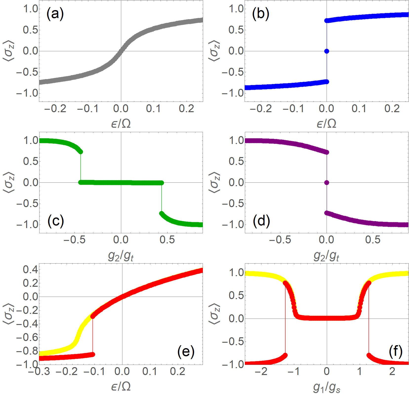
Figure 1: (color online) Different patterns of symmetry breaking. (a-f) Spin expectation $\langle\sigma_{z}\rangle$ in the cases of (a) paramagnetic-like, (c) antiferromagnetic-like, (b,d) the spontaneous symmetry breaking, (e) paramagnetic+first/second-order-transition and (f) antiferromagnetic+first/second-order-transition. These cases are illustrated by fixed parameters at $g_{2}=0$ with $g_{1}=0.9g_{\mathrm{s}}$ (a) or $g_{2}=0$ (b), at $\epsilon=0$ with $g_{1}=0.9g_{\mathrm{s}}$ (c) or $g_{1}=1.2g_{\mathrm{s}}$ (d), at $g_{1}=0.7g_{\mathrm{s}}$ (e) with $g_{2}=0.6g_{\mathrm{t}}$ (green) or $g_{2}=0.65g_{\mathrm{t}}$ (red), at $\epsilon=1g_{\mathrm{t}}$ (f) with $g_{2}=-0.02g_{\mathrm{t}}$ (green) or $g_{2}=0.02g_{\mathrm{t}}$ (red), given a frequency $\omega=0.001\Omega$.

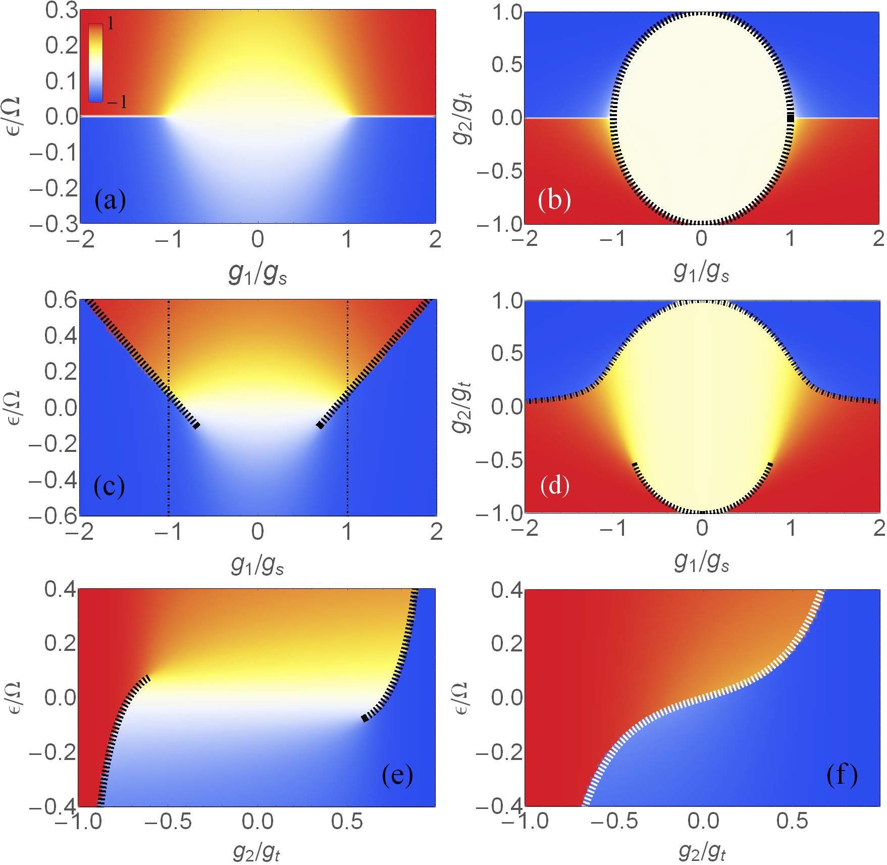
Figure 2: (color online) Phase diagrams and analytic phase boundaries in low frequency limit. Spin expectation $\langle\sigma_{z}\rangle$ at a fixed parameter (a) $g_{2}=0$, (b) $\epsilon=0$, (c) $g_{2}=0.5g_{\mathrm{t}}$, (d) $\epsilon=10g_{\mathrm{t}}$, (e) $g_{1}=0.7g_{\mathrm{s}}$, (f) $g_{1}=1.2g_{\mathrm{s}}$. Here $\omega=0.01\Omega$. All panels share the same color legend for $\langle\sigma_{z}\rangle$ as (a). The dashed or dot-dashed curves are analytic boundaries (4) and (5), the vertical lines in (c) are marking $g_{\mathrm{s}}$ as a reference for the boundary moving.

Either the bias and the nonlinear interaction will break the parity symmetry of the linear QRM $H_{0}$. Interestingly different scenarios arise in the interplay of linear coupling with the bias and the nonlinear interaction, leading to various patterns of symmetry breaking. On the one hand, the linear QRM has a critical point at $g_{1}=g_{\mathrm{s}}\equiv\sqrt{\omega\Omega}/2$ which also turns out to be a critical point for change of symmetry-breaking patterns (though, by a perspective view in Section IV, this pattern critical point may be shifted when both the bias and the nonlinear interaction are present). The regimes below and above the critical point respond to the symmetry breaking with completely different sensitivities. On the other hand, within a same linear-coupling regime, the processes of symmetry breaking may be essentially different in the presence of the bias and nonlinear interaction.

Fig.1 illustrates the different patterns of symmetry breaking in response to the bias and the nonlinear interaction, as calculated from exact diagonalization. Fig.1 (a) shows the evolution of the spin expectation $\left\langle\sigma_{z}\right\rangle$ with respect to the variation of the bias, below $g_{\mathrm{s}}$ of linear coupling and in the absence of the nonlinear interaction. We see that the amplitude of $\left\langle\sigma_{z}\right\rangle$ increases gradually with the bias strength, which is paramagnetic-like. Fig.1 (c) shows the dependence of $\left\langle\sigma_{z}\right\rangle$ on the strength of the nonlinear interaction below $g_{\mathrm{s}}$. We see that $\left\langle\sigma_{z}\right\rangle$ has no response to the nonlinear interaction $g_{2}$ and remains vanishing until the strength of $g_{2}$ reaches some critical point $g_{2c}$. Once $g_{2}$ goes beyond $g_{2c},$ the spin expectation $\left\langle\sigma_{z}\right\rangle$ jumps abruptly to a finite value and then starts approaching to saturation. This pattern with a threshold for polarization is antiferromagnetic-like. We see the essentially different patterns of symmetry breaking: there is a first-order phase transition induced by the nonlinear interaction, while there is no transition in introducing the bias. Above the critical point $g_{\mathrm{s}}$ of the linear coupling, both the bias and nonlinear interaction bring another pattern. In Fig.1 (b,d), we see that a tiny strength of either the bias or the nonlinear coupling will lead to dramatic change in $\left\langle\sigma_{z}\right\rangle$ which jumps to a finite value. This is the pattern of spontaneous symmetry breaking. This means the system is extremely sensitive to the perturbation of the bias or the nonlinear interaction, in a sharp contrast to both the paramagnetic-like pattern and antiferromagnetic-like pattern. Furthermore, as in Fig.1 (e), the interplay of the bias and the nonlinear interaction may lead to a paramagnetic-like pattern followed by a second-order-like transition (green line) or first-order transition (red line) . It is also interesting to see that in the interplay with both the bias and nonlinear interaction increasing $g_{1}$ could bring about an antiferromagnetic-like pattern but with the afore-mentioned first-order transition replaced by a second-order transition, as illustrated by the green line in Fig.1 (f). This occurs for the opposite signs of the bias and the nonlinear interaction. When the signs are the same another pattern could emerge, i.e. antiferromagnetic-like pattern plus successive transitions of second-order and first-order kinds, as shown by the red line in Fig.1 (f).

IV Phase diagrams and analytic transition boundaries in the low frequency limit

To get a perspective view we plot the phase diagrams in the full parameter spaces, as in Fig. 2. Panels (a) shows the dependence of $\left\langle\sigma_{z}\right\rangle$ on the bias and the linear coupling, in the absence of the nonlinear interaction. The spin expectation $\left\langle\sigma_{z}\right\rangle$ has a positive value in the red region for $\epsilon>0$ and a negative value in the blue region for $\epsilon<0$. The white line at $\epsilon=0,$ with vanishing $\left\langle\sigma_{z}\right\rangle,$ is parity-symmetry line from the conventional QRM. As we see, for the weak linear coupling regime $\left|g_{1}\right|<\left|g_{\mathrm{s}}\right|,$ when the bias is getting stronger, the color gradually turns from white to red or blue, which indicates no phase transition. Differently, for the whole strong coupling regime $\left|g_{1}\right|>\left|g_{\mathrm{s}}\right|$, there is a sharp color change across the parity-symmetry line, indicating the spontaneous symmetry breaking. Panel (b) shows the behavior of $\left\langle\sigma_{z}\right\rangle$ in the interplay of the nonlinear interaction and the linear coupling in the absence of the bias. We see that, besides the parity-symmetry white line at $g_{2}=0$, another white round region is opened where the parity symmetry for the ground state is also unbroken. The antiferromagnetic-like pattern occurs in the regime of the round region. The dashed line along the circumference of the round region in panel (b) is the analytic boundary

$$\left|g_{1c}\right|=g_{\mathrm{s}}\sqrt{1-\widetilde{g}_{2}^{2}/g_{\mathrm{t}}^{2}}$$ (3)

where $\widetilde{g}_{2}=\left(1+\chi\right)g_{2}$, which reproduces the numerical boundary.

Fig. 2 (c,d) illustrate the mutual influence of the bias and the nonlinear interaction over their phase diagrams. Panel (c) is plotted in the dimensions of the bias and the linear coupling, in the presence of a finite nonlinear interaction $g_{2}=0.7g_{\mathrm{t}}.$ Here $g_{\mathrm{t}}=\omega/2$ is the physical limit for the nonlinear interaction, beyond the limit the system energy becomes negatively unbound thus being unphysical. We see that, in the presence of a finite nonlinear interaction, the boundary of $\left\langle\sigma_{z}\right\rangle$ gets tilted from the horizontal line in zero-$g_{2}$ case. Furthermore, the transition boundary enters the regime $[-g_{\mathrm{s}},g_{\mathrm{s}}]$ where originally there is no transition in the absence of the nonlinear interaction. Panel (d) is plotted in the $g_{1}$-$g_{2}$ section in the presence of a finite strength of the bias $\epsilon=0.1\Omega.$ We see for $g_{2}>0$ the connection of the circle and the horizontal line originally in $\epsilon=0$ case (panel (b)) now becomes round, with the boundary changing from a dome shape to be a hill shape. In this reshaping the transition at the boundary remains to be first-order. For $g_{2}<0,$ some section of the first-order round boundary disappears, with the jump of $\left\langle\sigma_{z}\right\rangle$ closed and softened, turning the original half-circle boundary to be an arc shape. Let us label by $g_{2}^{\mathrm{E}}$ the critical nonlinear interaction for the ends of the arc boundary. The analytic expression of $g_{2}^{\mathrm{E}}$ will be given in Eq.(28) and the dependence on the bias strength plotted in Fig.15(b) in Section X.1. Meanwhile, the arc spanning angle gets narrower than the half circle, i.e., $\left|g_{1c}\right|$ is smaller at the same value of $g_{2}$. The rest first-order arc boundary, remaining in the large-$g_{2}$-amplitude regime, shrinks with an enhanced bias.

Fig. 2 (e,f) show the phase diagrams at a fixed linear coupling below $g_{\mathrm{s}}$ (panel (e)) or above $g_{\mathrm{s}}$ (panel (f)). Below $g_{\mathrm{s}}$ there are two first-order boundaries in the variations of the bias and the nonlinear interaction, which are separated. When the linear coupling get stronger the two boundaries are curved, with their ends getting closer and finally connected to form one first-order boundary above $g_{\mathrm{s}}$.

For a quantitative description, we extract the analytic boundary marked by $g_{1c}$ or $\epsilon_{c}$ as follows

$$\left|g_{1c}\right| = g_{\mathrm{s}}[1+\frac{g_{\mathrm{t}}\epsilon}{\widetilde{g}_{2}\Omega}]\sqrt{1-\widetilde{g}_{2}^{2}/g_{\mathrm{t}}^{2}},$$ (4)

$$\epsilon_{c} = \frac{\widetilde{g}_{2}}{g_{\mathrm{t}}}[\frac{\left|g_{1}\right|/g_{\mathrm{s}}}{\sqrt{1-\widetilde{g}_{2}^{2}/g_{\mathrm{t}}^{2}}}-1]\ \Omega.$$ (5)

We leave the analytic derivation in Section X.1. Note here, whereas for $g_{\mathrm{t}}\epsilon>0$ the extension of boundary is unlimited, for $g_{\mathrm{t}}\epsilon>0$ the validity regime is $\left|g_{2}\right|<g_{2}^{\mathrm{E}}$ which is the arc boundary. We leave the detail of derivations in Section X. Setting $\epsilon=0$ retrieves the round boundary $\left|g_{1c}\right|=g_{\mathrm{s}}\sqrt{1-\widetilde{g}_{2}^{2}/g_{\mathrm{t}}^{2}}$ in the absence of bias Ying-2018-arxiv . We plot the analytic boundaries by the dashed or dot-dashed lines in Fig. 2 (b-f), which are in good agreements with the numerical boundaries.

V Tricriticality-(i) in the low frequency limit

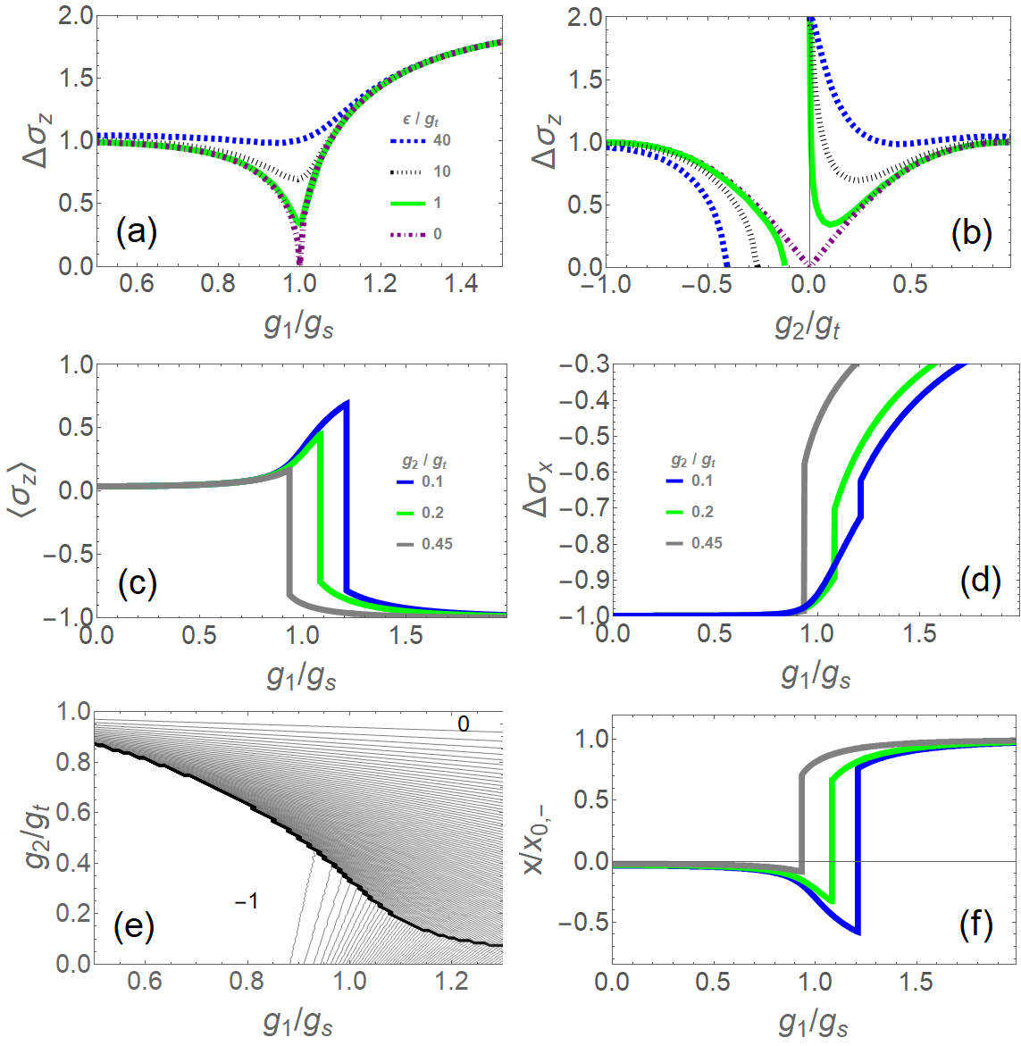
Figure 3: (color online) Tricriticality-(i) in low frequency limit. (a) Spin expectation discontinuity $\Delta\sigma_{z}$ along the transition boundary in $g_{2}>0$ regime as a function of $g_{1}$ for $\epsilon=0g_{\mathrm{t}}$ (purple dot-dashed), $1g_{\mathrm{t}}$ (green solid), $10g_{\mathrm{t}}$ (black dotted) and $40g_{\mathrm{t}}$ (blue dashed) at $\omega=0.001\Omega$. (b) $\Delta\sigma_{z}$ as a function of $g_{2}$. (c-f) Three-phase behavior of $\langle\sigma_{z}\rangle$ (c), $\langle\sigma_{x}\rangle$ (d,e), $\langle\widehat{x}\rangle$ (f) for $\epsilon=40g_{\mathrm{t}}$. (c,d,f) give illustrations with fixed $g_{2}=0.1g_{\mathrm{t}}$ (blue), $g_{2}=0.2g_{\mathrm{t}}$ (green) and $g_{2}=0.45g_{\mathrm{t}}$ (gray), while (e) is a contour plot.

In Fig. 2(b) one may notice on each side $g_{1}=\pm g_{\mathrm{s}}$ is a tricritical point where the round boundary and horizontal line are crossing. In Fig. 3(a) by the purple dot-dashed line we show the spin expectation discontinuity $\Delta\sigma_{z}$, i.e. the jump of $\langle\sigma_{z}\rangle$ across the boundary, with the finite value of $\Delta\sigma_{z}$ representing the first-order transition. The transition becomes second-order at $g_{\mathrm{s}}$ as indicated by the vanishing of $\Delta\sigma_{z}$.  In the presence of the bias, this second-order transition also turns to be first-order, as we illustrate by $\epsilon/\Omega=0.001$, $0.01$ and $0.04$ in the low frequency limit ($\epsilon/g_{\mathrm{t}}=1,$ $10$ and $40$ if taking $\omega=0.001\Omega$). With the bias increasing, the shape of the $\Delta\sigma_{z}$ minimum evolves from a sharp dip into a round valley. Fig. 3(b) provides a view of $\Delta\sigma_{z}$ in the $g_{2}$ dimension, which includes both boundaries in the positive and negative $g_{2}$ regimes. The $\langle\sigma_{z}\rangle$-vanishing point at zero bias is extending into a window at finite biases. In the negative $g_{2}$ regime the remaining finite-$\langle\sigma_{z}\rangle$ section in panel (b) corresponds to the boundary arc.  In the positive $g_{2}$ regime, it is worthwhile to follow the evolution of the minimum position $\Delta\sigma_{z}$, which is moving away from the original point $g_{2}=0$. As afore-mentioned, this minimum point is originally a tricritical point in the absence of the bias, now in the presence of the bias it turns out to be an imprint of new tricriticality.

Indeed, when scanning $g_{1}$ in Fig. 3(c), as demonstrated by the case $g_{2}=0.1g_{\mathrm{t}}$ (blue line) we see a three-phase-like scenario: firstly a flat region in spin expectation $\langle\sigma_{z}\rangle$, secondly a fast-rising region, finally jumping into a region with opposite sign. The three phases look more distinct in the evolution of the spin expectation in $x$ direction, $\langle\sigma_{x}\rangle,$ as shown by the blue line in Fig. 3(d). Essential changes of the three phases may be indicated by $\langle a^{+}+a\rangle$ which is effective spatial particle position $x$ (we shall discuss more in Sections VIII and IX). As shown in Fig. 3(f), the effective particle resides closely around the origin in the first phase, moves obviously away from origin in the second phase and jumps abruptly to the other side in the third phase. These three phases are separated by two transition-like points, the first transition is second-order-like and the second one is of first order. When the bias strength increases, the two transitions get closer to each other and finally meet, as illustrated by $g_{2}=0.2g_{\mathrm{t}}$ (green lines) and $g_{2}=0.45g_{\mathrm{t}}$ (gray lines) in Fig. 3(c,d,f). Such a scenario of two separate transitions converging to one transition forms a tricritical-like point, which can be seen more clearly by the contour plot of $\langle\sigma_{x}\rangle$ in Fig. 3(e). This tricritical-like point is located around the afore-mentioned $\Delta\sigma_{z}$ minimum position.

VI Novel tricriticalities at finite frequencies

The low frequency limit discussed in previous sections is also the semiclassical limit, as the wave-packet size is so small that it can be regarded as a semiclassical mass point (see Section IX.1).  In such a semiclassical limit,  in each quadrant of the phase diagram the nonlinear interaction induces only one transition in the absence of the bias and at most two transitions in the interplay with the bias. On the other hand, the spontaneous symmetry breaking occurs immediately upon any tiny strength of the bias or nonlinear interaction. In this section, we shall see that the full quantum-mechanical effect at finite frequencies will change this picture and lead to richer scenarios. We find that additional transitions appear, novel tricriticalities arise and the spontaneous symmetry breaking exhibits a fine structure.

VI.1 Additional transition and Tricriticality-(ii) induced by the frequency respectively in the bias or the non-linear interaction

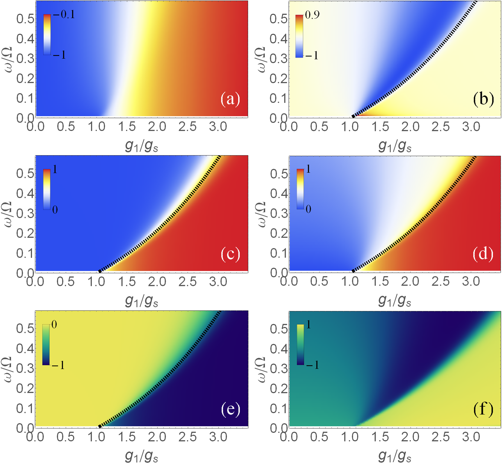
Figure 4: (color online) Tricriticality-(ii) induced by frequency $\omega$. Phase diagrams of different quantities by frequency variation ($\omega$) at $\epsilon=0.001g_{\mathrm{t}}$ with $g_{2}=0$ (a,c,e) and $g_{2}=0.0001g_{\mathrm{t}}$ with $\epsilon=0$ (b,d,f) for (a) $\langle\sigma_{x}\rangle$, (b) $\langle\hat{x}\rangle_{+}$, (c) $\langle\sigma_{z}\rangle$, (d) $\langle\hat{x}\rangle_{-}/|x_{0,-}|$ ($\hat{x}=(a+a^{\dagger})/\sqrt{2}$), (e) $\langle\hat{x}\rangle/|x_{0,+}|$, (f) $\tilde{x}_{+}=\langle\hat{x}\rangle_{+}/(|x_{0,+}|\rho_{+})$. The dashed lines in (b-e) are $g^{\mathrm{II}}_{1c}$ extracted from analytic Eqs.(6) and (7).

The tricriticality in Section V occurs in the low frequency limit. The transitions and the tricriticality arise from the competition and interplay of the bias, the nonlinear interaction and the linear coupling. In such a situation, different physical quantities exhibit imprints of each transition at a same transition point, as one can see from Fig. 3(c,d,f). Here we show another kind of tricriticality induced by the frequency which has a different nature and transition positions diverge for different physical quantities.

In Fig.4, we show a variety of physical quantities with the dependence on the frequency $\omega$, under a fixed bias $\epsilon=0.1\Omega$ in panels (a,c,e) or a fixed nonlinear interaction $g_{2}=0.01g_{\mathrm{t}}$ in panels (b,d,f). The two parameter cases have similar behavior despite some detail and sign difference for some quantities. As expected, in the low frequency limit both $\langle\sigma_{x}\rangle$ (panel (a)) and $\langle\sigma_{z}\rangle$ (panel (c)) show one transition at a same point around $g_{1}=g_{\mathrm{s}}$. However, when the frequency is raised, $\langle\sigma_{x}\rangle$ and $\langle\sigma_{z}\rangle$ respond differently. In fact, the transition in $\langle\sigma_{x}\rangle$ is not much affected by the frequency except for some softening of the transition, whereas the transition in $\langle\sigma_{z}\rangle$ is moving obviously toward the larger-$g_{1}$ direction. The diverging evolutions of the transition positions of $\langle\sigma_{x}\rangle$ and $\langle\sigma_{z}\rangle$ indicate an additional transition induced by the finite frequency, thus the one transition in the low-frequency limit becomes two transitions at finite frequencies. It also seems peculiar that the spin expectations $\langle\sigma_{x}\rangle$ and $\langle\sigma_{z}\rangle$ respond to the two transitions respectively: the first transition induces response in $\langle\sigma_{x}\rangle$ but leaves no imprints in $\langle\sigma_{z}\rangle$, while the second transition releases a strong onset signal in $\langle\sigma_{z}\rangle$ but gives no sign in $\langle\sigma_{x}\rangle.$ This additional transition can also be seen from the effective particle position or displacement $\langle\widehat{{x}}{\rangle=}\langle{a^{{\dagger}}+a\rangle/}\sqrt{2}$, as shown in Fig.4(c).

The two diverging transitions can be also detected simultaneously by a single physical quantity, such as the spin-filtered displacement $\langle\widehat{{x}}{\rangle}_{\pm}{=}\langle{a^{{\dagger}}+a\rangle}_{\pm}{/}\sqrt{2}$ which only counts the contribution from one spin component, as shown in 4(b,d) where it is quite clear to visualize two boundaries corresponding to the two transitions. To have unified upper and lower bounds for plotting we also introduce the normalized spin-filtered displacement $\widetilde{x}_{\pm}=\langle{a^{{\dagger}}+a\rangle}_{\pm}/(\sqrt{2}\rho_{\pm}\left|x_{0,sign(-\widetilde{g}_{2})}\right|)$, where $\rho_{\pm}=\langle\psi^{\pm}|\psi^{\pm}\rangle=\left(1\pm\left\langle\sigma_{z}\right\rangle\right)/2$ is the spin-component weight and $x_{0,\pm}=\mp g_{1}^{\prime}/(1\pm\widetilde{g}_{2}^{\prime})$ is the potential displacement (see Section IX). Here we have defined $g_{1}^{\prime}=\sqrt{2}g_{1}/\omega\$ and $\widetilde{g}_{2}^{\prime}=2\widetilde{g}_{2}/\omega$. Besides the normalization, $\widetilde{x}_{\pm}$ have another convenience that it has three regimes of values respectively for the three phases separated by the two transitions. Thus the three phases can can be distinguished by three colors, as shown in Fig.4(f). It should be mentioned that at higher frequencies there is some discrepancy for the second transition point from$\ \widetilde{x}_{\pm}$. This spurious transition discrepancy is simply coming from the cancellation effect around the transition from its numerator $\langle{a^{{\dagger}}+a\rangle}_{\pm}$ and denominator $\rho_{\pm}$, while separately both $\langle{a^{{\dagger}}+a\rangle}_{\pm}$ and $\rho_{\pm}$ have the right second transition point.  Nevertheless, the discrepancy at low frequencies is negligible so we can still use it for further discussions by the advantages of its normalization and value(color)-phase correspondence.

Reversely in lowering the frequency, the two boundaries of the three phases will converge to one point, thus forming a new triple point and another kind of tricriticality. Conventionally a tricriticality is composed of three critical boundaries, while this tricriticality here is comprised of two critical boundaries at finite frequencies and one critical point at zero frequency. This critical point connects two phases which does not adjoin directly through either of the other two boundaries. Thus there are three kinds of critical behavior. In this sense we still term it as a tricriticality. It should be noted that the tricriticality of this case, as labeled by (ii), is distinguished from Tricriticality-(i) in Section V. Tricriticality-(i) happens in the presence of both the bias and the nonlinear interaction, while Tricriticality-(ii) here occurs in the respective presence of the bias or the nonlinear interaction. From the mechanism clarification in Section IX we will see that the additional transition and new tricriticality originate from a full-quantum-mechanical effect, in a contrast to the semiclassical effect in the low frequency limit.

VI.2 Tricriticality-(iii) induced by the bias or the nonlinear interaction at finite frequencies

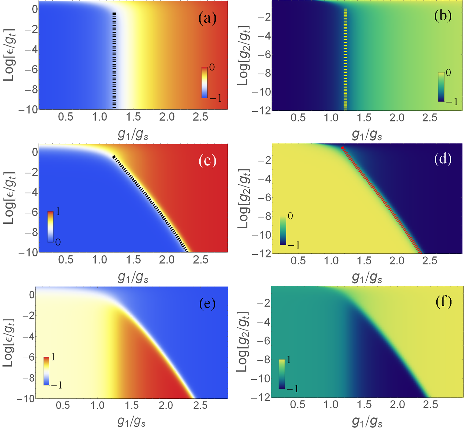
Figure 5: (color online) Tricriticality-(iii) induced by the bias or the nonlinear interaction at a finite frequency. Phase diagrams at $\omega=0.1\Omega$ for variation of $\epsilon$ at $g_{2}=0$: (a) $\langle\sigma_{x}\rangle$, (c) $\langle\sigma_{z}\rangle$, (e) $\widetilde{x}_{-}$. Phase diagrams for variation of $g_{2}$ at $\epsilon=0$: (b) $\langle\sigma_{x}\rangle$, (d) $\langle\sigma_{z}\rangle$, (f) $\widetilde{x}_{+}$. The dot-dashed lines in (a,b) are analytic $g_{1c}^{\mathrm{I}}$ and the dashed lines in (c,d) are analytic $\epsilon_{c}^{\mathrm{II}}$ and $g_{2c}^{\mathrm{II}}$ in Eqs. (6) and (7)

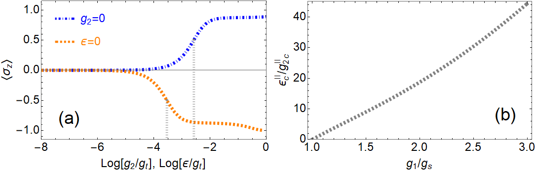
Figure 6: (color online) Sensitivity competition for spontaneous symmetry breaking. (a) $\langle\sigma_{z}\rangle$ depending on $\epsilon$ at $g_{2}=0$ (orange dashed) and on $g_{2}$ at $\epsilon=0$ (blue dot-dashed) at $g_{1}=1.5g_{\mathrm{s}}$ and $\omega=0.1\Omega$. (b) Threshold ratio $\epsilon_{c}^{\mathrm{II}}/g_{2c}^{\mathrm{II}}$ depending on $g_{1}$

It will provide another view by fixing a finite frequency and varying the bias or the nonlinear interaction. As described in Section IV, in the low frequency limit we see from Fig. 2 (a,b) that in each quadrant of the phase diagrams there is no more than one transition. As revealed in Section VI.1, at a finite frequency the single transition turns to be two successive transitions. The variation of the bias or the nonlinear interaction will influence the transitions and induce a third tricriticality which we label by Tricriticality-(iii).

The successive transitions can be seen more clearly from a zoom-in view by a logarithm scale for the variations of $\epsilon$ and $g_{2},$ as illustrated by Fig.5 at a finite frequency $\omega=0.1\Omega$. Panels (a,c,e) present the phase diagrams for the pure bias dependence without the nonlinear interaction and panels (b,d,f) for the nonlinear interaction in the absence of the bias. To distinguish the two transitions we label the transition in $\langle\sigma_{x}\rangle$ by $g_{1c}^{\mathrm{I}}$ and that in $\langle\sigma_{z}\rangle$ by $g_{1c}^{\mathrm{II}}.$ We see in panels (a,b) that the first transition in $\langle\sigma_{x}\rangle$ does not vary at weak strengths of $\epsilon$ or $g_{2}$, except that the transition point at low frequencies shifts a bit from $g_{1c}\sim g_{\mathrm{s}}$ to $g_{1c}^{\mathrm{I}}\approx\sqrt{\omega^{2}+\sqrt{\omega^{4}+g_{\mathrm{s}}^{4}}}$Ying2015 due to the width of wave packet in the wave-packet splitting.  In a sharp contrast, the second transition is very sensitive to the variation of the bias and the nonlinear interaction. In fact, as demonstrated by Fig.5(c,d), the transition point $g_{1c}^{\mathrm{II}}$ has an exponential dependence on $\epsilon$ and $\Omega$. Analytically we find the second boundary as a function of $g_{1}$ (see the derivation in Section X):

$$\left|\epsilon_{c}^{\mathrm{II}}\right| = \frac{(1-t)\Omega}{4\delta_{c}\zeta}\exp[-\frac{\zeta^{2}\overline{g}_{1}^{2}\Omega}{2\omega}],\quad\text{for }g_{2}=0,$$ (6)

$$\left|\widetilde{g}_{2c}^{\mathrm{II}}\right| = \frac{(1-t)g_{\mathrm{t}}}{\delta_{c}\zeta^{3}\overline{g}_{1}^{2}}\exp[-\frac{\zeta^{2}\overline{g}_{1}^{2}\Omega}{2\omega}],\quad\text{for }\epsilon=0,$$ (7)

where $\ \overline{g}_{1}\equiv g_{1}/g_{\mathrm{s}}$, $\delta_{c}=e^{-1},$ $t=(1-\zeta)^{2}/2+\omega/(\overline{g}_{1}^{2}\Omega)$ and $\zeta=(1-\overline{g}_{1}^{-4})^{1/2}$. The analytic boundaries $\epsilon_{2c}^{\mathrm{II}}$ and $g_{2c}^{\mathrm{II}}$ are plotted as the dashed lines in Fig.5(c,d), in good agreements with the numerical results.

With the strength increase of the bias or the nonlinear interaction, the two transitions respectively reflected in $\langle\sigma_{x}\rangle$ and $\langle\sigma_{z}\rangle$  are getting closer and finally meet to form Tricriticality-(iii). A better view of this tricriticality can be obtained from $\widetilde{x}_{\pm}$ as in Fig.5(e,f) where three phases are distinctly represented by three colors. Above the tricritical point it is one transition of first-order type, while below the tricritical point the transition is bifurcated into a second-order-like transition and a first-order-like one. Exactly speaking, in the bias case the transition above the tricritical point is a short extension from the first-order transition below the tricritical point. This transition soon gets softened and fades away when the linear coupling $g_{1}$ is reduced to below $g_{\mathrm{s}}$. In the nonlinear interaction case, the first-order-like transition covers the entire $g_{2}$ regime thus also the whole $g_{1}$ regime.

To distinguish from Tricritcalities (i) and (ii) let us mention the difference. Tricritcality-(i) in the low frequency limit revealed in Section V occurs in the presence of both the bias and the nonlinear interaction. Tricriticality-(iii) here needs only the bias or the nonlinear interaction. Tricriticality-(ii) unveiled in Section VI.1 is induced by the variation of the frequency, here Tricriticality-(iii) is induced by the bias or nonlinear interaction at a fixed finite frequency.

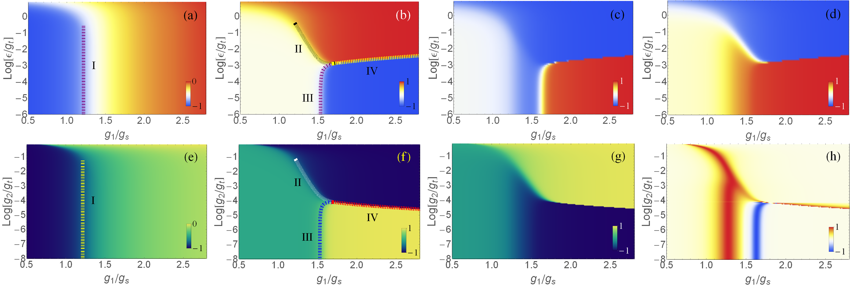
Figure 7: (color online) Tricriticality-(iv) with two tricritical-like points in the interplay of the bias the nonlinear interaction. Phase diagrams at $\omega=0.1\Omega$ for variation of $\epsilon$ at $g_{2}=10^{-4}g_{t}$: (a) $\langle\sigma_{x}\rangle$, (b) $\langle\sigma_{z}\rangle$, (c) $\widetilde{x}_{+}$, (c) $\widetilde{x}_{-}$. Density plot for variation of $g_{2}$ at $\epsilon=10^{-3}g_{t}$: (e) $\langle\sigma_{x}\rangle$, (f) $\langle\sigma_{z}\rangle$, (g) $\widetilde{x}_{+}$, (h) $d\widetilde{x}_{-}/dg_{1}$ scaled by the local peak amplitude. The lines are our analytic $g_{1c}^{\mathrm{I}}$ in panels (a,e), $\epsilon_{c}^{\mathrm{II}}$, $\epsilon_{c}^{\mathrm{III}}$, $\epsilon_{c}^{\mathrm{IV}}$ in panel (b) and $g_{2c}^{\mathrm{II}}$ $g_{2c}^{\mathrm{III}}$, $g_{2c}^{\mathrm{IV}}$ in panel (f) (see Eqs. (9)- (14)).

The scenario of Tricriticality-(iii)  also gives rise to a fine structure of the spontaneous symmetry breaking for the finite frequency case. Note that the negative-$\epsilon$/$g_{2}$ regime has the same tricritical scenario, except for being antisymmetric for $\langle\sigma_{z}\rangle$ and symmetric for $\langle\sigma_{z}\rangle$ in the quadrants of the phase diagrams. Thus, rather than an immediate jump of $\langle\sigma_{x}\rangle$ from zero to a finite value upon the opening of the bias or the nonlinear interaction, there is now a window within which the parity symmetry of the ground state is maintained to some large extent, as indicated by the vanishing $\langle\sigma_{z}\rangle$. Out of the window the symmetry is broken. This window becomes narrower when the linear coupling gets stronger, but can be widened by a higher frequency.

VI.3 Sensitivity competition of the bias and the nonlinear interaction in spontaneous symmetry breaking

The spontaneous symmetry breaking means that the symmetry is vulnerable to the perturbation of the bias or the nonlinear interaction. It may be worthwhile to compare the symmetry-breaking sensitivity to the bias and the nonlinear interaction. As described in the paramagnetic-like and antiferromagnetic-like symmetry patterns, let us remind that in the weak linear coupling regime $g_{1}<g_{\mathrm{s}}$ the polarization $\langle\sigma_{z}\rangle$ is more sensitive to the bias but responseless to the nonlinear interaction within a threshold $g_{2c}$. We find this sensitivity tendency is reversed in the strong linear coupling regime $g_{1}>g_{\mathrm{s}}$. It turns out that in this regime the symmetry breaking finds a higher sensitivity to the nonlinear interaction than the bias. In Fig. 6(a), we demonstrate that the symmetry breaking occurs earlier in the nonlinear interaction (orange dashed line, $\epsilon=0$) in the sense that the bias needs to have a relatively stronger strength (blue dot-dashed line, $g_{2}=0$) to bring about the transition. Fig. 6(b) shows the ratio of the critical-like strengths between the bias and the nonlinear interaction. One sees the critical strength of the bias is one or two orders larger than the nonlinear interaction. Moreover, this ratio is growing with the linear coupling $g_{1}$.

One can see more clearly from the analytic boundary expressions (6) and (7). We obtain the ratio between the critical bias and nonlinear interaction

$$\frac{\left|\epsilon_{c}^{\mathrm{II}}\right|}{\left|\widetilde{g}_{2c}^{\mathrm{II}}\right|}=\frac{\zeta^{2}\overline{g}_{1}^{2}\Omega}{4g_{\mathrm{t}}}.$$ (8)

On the one hand, the low frequency contributes to the order difference as $g_{\mathrm{t}}=\omega/2.$ On the other hand, the ratio is proportional to $\overline{g}_{1}^{2}$ which grows parabolically with the strength of the linear coupling. In addition, $\zeta$ starts for a small value at $g_{1}=g_{\mathrm{s}}$ and soon approaches to the value $1$ in the increase of $g_{1}$, which also contributes to the ratio growing at the beginning. Thus, unlike in the regime below $g_{\mathrm{s}}$, the parity symmetry in the regime beyond $g_{\mathrm{s}}$ is more sensitively broken by the perturbation of nonlinear interaction than that of the bias, unless nearby $g_{\mathrm{s}}$. This sensitivity priority of the nonlinear interaction comes from the entanglement of the nonlinear interaction and the linear coupling, as will be indicated by Eq.(19) in Section IX.

VI.4 Tricriticality-(iv) induced by the interplay of the bias and the nonlinear interaction at finite frequencies

In Tricriticality-(iii) we have considered the bias and the nonlinear interaction respectively. Now we should address how the tricritical point and the fine structure of spontaneous symmetry breaking are affected by the interplay of the bias and nonlinear interaction. In Fig. 7 we illustrate in panels (a-d) the phase diagrams by variation of the bias in the presence of a fixed nonlinear interaction, and in panels (e-h) the phase diagrams by variation of the nonlinear interaction in the presence of a fixed bias. As one can see, besides the transition boundaries I and II, two more boundaries appear as we mark by III and IV. As expected, the onset of transition I can be seen by the start of increasing in $\langle\sigma_{x}\rangle$, as shown in panels (a,e). Transitions II, III and IV can be clearly observed in $\langle\sigma_{z}\rangle$ as demonstrated in panels (b,f).

Although transition I is missed by $\langle\sigma_{z}\rangle$, all the transitions I-IV leave some imprints in $\widetilde{x}_{\pm}$ as in panels (c,d,g). The boundaries can also be all visualized by the peaks of the susceptibility $d\widetilde{x}_{\pm}/dg_{1}$, as illustrated in panel (h). For a fixed nonlinear interaction in panel (b-d), the boundary IV is tilted upwards, with the critical bias increasing with the linear coupling. For a fixed bias in panel (f-h), the boundary IV is tilted downwards, with the critical nonlinear interaction decreasing with the linear coupling.

In Fig. 7 the crossing of the boundaries I and II forms a first tricriticality around $g_{1}=1.2g_{\mathrm{s}},$ which actually is tricriticality-(iii) in the presence of only the bias or the nonlinear interaction. Now in the presence of both the bias and the nonlinear interaction, with the enhancement of the linear coupling the boundaries II and III get closer to the tilted boundary IV and seem to form a second tricritical-like point around $g_{1}=1.6g_{\mathrm{s}}$ which we label by Tricriticality-(iv).

We extract in the leading order the analytic boundaries expressed by the bias as a function of the linear coupling and the nonlinear interaction

$$\epsilon_{c}^{\mathrm{II}} = \frac{(1-t)\Omega}{4\delta_{c}\zeta}\exp[-\frac{\zeta^{2}\overline{g}_{1}^{2}\Omega}{2\omega}]+\frac{1}{4}\zeta^{2}\overline{g}_{1}^{2}\overline{g}_{2}\Omega,$$ (9)

$$\epsilon_{c}^{\mathrm{III}} = -\frac{(1-t)\Omega}{4\delta_{c}\zeta}\exp[-\frac{\zeta^{2}\overline{g}_{1}^{2}\Omega}{2\omega}]+\frac{1}{4}\zeta^{2}\overline{g}_{1}^{2}\overline{g}_{2}\Omega,$$ (10)

$$\epsilon_{c}^{\mathrm{IV}} = \frac{1}{4}\zeta^{2}\overline{g}_{1}^{2}\overline{g}_{2}\Omega,$$ (11)

or tracked by the nonlinear interaction in variations of the linear coupling and the bias

$$\widetilde{g}_{2c}^{\mathrm{II}} = \frac{(1-t)g_{\mathrm{t}}}{\delta_{c}\zeta^{3}\overline{g}_{1}^{2}}\exp[-\frac{\zeta^{2}\overline{g}_{1}^{2}\Omega}{2\omega}]+\frac{4\epsilon}{\zeta^{2}\overline{g}_{1}^{2}\Omega}g_{\mathrm{t}},$$ (12)

$$\widetilde{g}_{2c}^{\mathrm{III}} = -\frac{(1-t)g_{\mathrm{t}}}{\delta_{c}\zeta^{3}\overline{g}_{1}^{2}}\exp[-\frac{\zeta^{2}\overline{g}_{1}^{2}\Omega}{2\omega}]+\frac{4\epsilon}{\zeta^{2}\overline{g}_{1}^{2}\Omega}g_{\mathrm{t}},$$ (13)

$$\widetilde{g}_{2c}^{\mathrm{IV}} = \frac{4\epsilon}{\zeta^{2}\overline{g}_{1}^{2}\Omega}g_{\mathrm{t}},$$ (14)

where $\overline{g}_{2}=\widetilde{g}_{2}/g_{\mathrm{t}}$. As shown in Fig. 7(b,f) the analytic boundaries match the numerical ones fairly well.  We see that the interplay of the bias and the nonlinear interaction contributes to the second term of the boundaries II and III, as an additional term to (6) and (7). Exactly speaking, since the second term is equal to $\epsilon_{c}^{\mathrm{IV}}$ or $\widetilde{g}_{2c}^{\mathrm{IV}},$ the mathematical tricritical point (iv) is at the infinity of linear coupling. However in reality, although boundary IV is actually comprised of boundaries II and III with $\widetilde{g}_{2c}^{\mathrm{IV}}$ or $\epsilon_{c}^{\mathrm{IV}}$ as their center, they are too close to be distinguished when the boundaries are tilted in the regime of the strong linear coupling. Thus, effectively tricriticality-(iv) appears at a finite value of the linear coupling.

VI.5 Tricriticality-(v) induced by frequency in the interplay of the bias and the nonlinear interaction

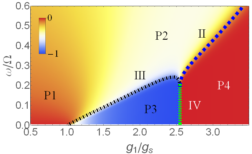
Figure 8: (color online) Tricriticality-(v): the second frequency-induced tricriticality. Phase diagram of $\langle\hat{x}\rangle_{+}/|x_{0,+}|$ in $g_{1}$-$\omega$ plane at $\epsilon=0.5\times 10^{-4}\Omega$ and $\log[g_{2}/g_{\mathrm{t}}]=-4.5$. P1, P2, P3 and P4 mark the different phases. The blue long-dashed, black dot-dashed and green dashed lines are analytic boundaries II, III and IV.

Now let us come back to the frequency dimension. In Section VI.1, we have seen that the frequency induces a tricritical point in the respective presence of the bias or the nonlinear interaction. Now we consider frequency effect in the presence of both the bias and the nonlinear interaction. Imagine we are standing at the boundary IV in Fig. 7, Eqs. (9)-(14) indicate that increasing the frequency would open the gap between the boundary IV and the boundaries II, III, thus inducing a tricritical-like behavior. We show such a scenario by Fig. 8 in the $g_{1}$-$\omega$ plane. As one can see, apart from the first frequency-induced tricritical point (tricriticality-(ii) as afore-labeled) around $g_{1}=1.0g_{\mathrm{s}},$ another tricritical-like point appears around $g_{1}=2.5g_{\mathrm{s}}$ which is the location of $g_{1c}^{\mathrm{IV}}$ at a fixed bias $\epsilon=0.0001\Omega$ and a nonlinear interaction $\log\left[g_{2}/g_{\mathrm{t}}\right]=-4.5$. More generally, from Eq. (14) we extract the location of the second frequency-induced tricriticality as

$$g_{1c}^{\mathrm{IV}}=g_{\mathrm{s}}\sqrt{\frac{2\epsilon+\sqrt{4\epsilon^{2}+\overline{g}_{2}^{2}\Omega^{2}}}{\Omega\overline{g}_{2}}}.$$ (15)

We label this tricriticality by (v).  Exactly speaking, this tricritical point is mathematically located at $\omega=0$, but effectively the tricriticality seems to form at some finite frequency as boundaries II and III are already too close to be distinguished at the finite frequency.

VI.6 Tendency for four successive transitions

From the discussions in Section V, we know that in the low frequency limit there are at most two transitions in increasing $g_{1}$. The various situations for the occurrence of tricriticality described above in Section VI demonstrate that finite frequencies can lead to three transitions. Still, it might be possible to go even further. A closer look at Fig. 8, we can see the boundaries II and III forms a dip shape around $g_{1}=2.5g_{\mathrm{s}}.$ The boundary III is actually a non-monotonic function of $g_{1}.$ Around $\omega=0.22\Omega,$ in fact increasing $g_{1}$ goes across the boundary III twice.  Let us mark the different phases by P1, P2, P3, P4. In increasing $g_{1}$ one starts with phase P1. After the first second-order transition the system enters phase P2. Then the first time across boundary III brings the system from phase P2 to phase P3. By the second time across boundary III the system re-enters Phase P2. After the short re-entrance of phase P2, the system transits to phase P4 through boundary II. Thus, in this regime the system actually experiences four successive transitions, i.e. transitions I, III, III and II, going through phases P1, P2, P3, P2, P4. This tendency of the second additional transition indicates that finite frequencies induces a subtle energy competition beyond the semiclassical picture.

VII Quadruple points and tetracriticality

In last section we have seen that at finite frequencies the system can have four phases P1, P2, P3 and P4 with three, even four transitions. We have addressed a variety of situations in which tricriticality may occur. Since we have four phases totally, one may wonder whether it is possible for all the four phases to meet and form a quadruple point. We find this can happen indeed. The possibility is indicated from the last transition point Eq. (6) which, if the bias $\epsilon$ is being reduced, approaches to the first transition $g_{1c}^{\mathrm{I}}=g_{\mathrm{s}}$ in the low frequency limit. This process of transition converging is shown in Fig. 9, where we set $\epsilon=0.0005g_{\mathrm{t}}$ which is proportional to the frequency. As one sees, all three transitions boundaries finally collapses to one point at $g_{1}=g_{\mathrm{s}}$, thus forming a quadruple point and a kind of tetracriticality. Again here, rather than four boundaries conventionally, the tetracriticality here consists of three critical boundaries at finite frequencies and one critical point at zero frequency. The critical point at zero frequency connects phases P1 and P4 directly.

The quadruple point is illustrated for a small value of $g_{2}$. One would also get similar quadruple points in other values of $g_{2}$. The track by varying $g_{2}$ continuously would yield a section of quadruple line along $\left|g_{1}\right|=g_{\mathrm{s}}\sqrt{1-\widetilde{g}_{2}^{2}/g_{\mathrm{t}}^{2}}$ which is actually the transition boundary (3) in the absence of the bias. Since the quadruple line is parabolic in small values of $\widetilde{g}_{2}$, in weak nonlinear interactions the quadruple points turn out to be around $\left|g_{1}\right|=g_{\mathrm{s}}$ in the leading order, as we have seen in the illustrated figure 9.

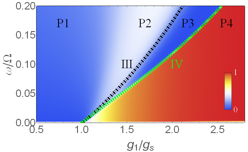
Figure 9: (color online) Quadruple point and tetracriticality. Phase diagram of $\langle\hat{x}_{-}\rangle/|x_{0,-}|$ in $g_{1}$-$\omega$ plane at $\log[g_{2}/g_{\mathrm{t}}]=-4.5$ with $\epsilon=0.0005g_{\mathrm{t}}$. In low frequency limit the four phases P1, P2, P3 and P4 meet around $g_{1}=g_{\mathrm{s}}$, forming a quadruple point and a tetracriticality.

VIII Changeovers of the wave function in the phase transitions

To see the essential changes of quantum state in the transitions we shall monitor the evolution of the wave function. In Fig.10 we show the spin-up and spin-down components of the wave function that goes through successive transitions in the variation of the linear coupling, under fixed values of bias and nonlinear interaction. Panel (a,b) are in the low frequency limit, while Panel (c)-(f) are finite-frequency cases. Note different choices of frequency will change $g_{\mathrm{t}}$ which is taken to be the strength reference of the nonlinear interaction as well as the bias. Nevertheless by fixing two ratios $\widetilde{g}_{2}/g_{\mathrm{t}}$ and $\epsilon/\Omega$ we have the same transition point of the last transition IV, around $g_{1}\sim 2.5g_{\mathrm{s}}$, which is the common one in the different frequency illustrations, as indicated by Eq.(15).

In the low frequency limit (illustrated by $\omega=0.001\Omega$) the wave packet is very thin, just like a mass point of an effective particle, as one sees from panels (a,b). Starting from $g_{1}=0$ till the first transition $g_{1}\sim 1.0g_{\mathrm{s}}$ the effective particle always stays at the origin $x=0.$ Beyond the first transition it starts to go away from the origin, and shifts to the other side at the next transition around $g_{1}\sim 2.5g_{\mathrm{s}}$.

At a finite frequency $\omega=0.1\Omega$ in panels (c,d) the wave packet is obviously broadened, but still remaining in a single-branch structure and staying around the origin before the first transition. After the first transition the wave packet splits into two branches in both the spin components, which is different from the low frequency limit. Strengthening more the linear coupling $g_{1}$ triggers the second transition around $g_{1}\sim 1.6g_{\mathrm{s}}$ where one branch of the wave packet is broken. In such a broken-branch state the wave packet on one side vanishes in both spin components and all the weight goes to the branch on the other side. Further increase of $g_{1}$ induces the third transition, around $g_{1}\sim 2.5g_{\mathrm{s}}$, which switches the broken-branch state from one side to the other side. These three successive transitions correspond to the boundaries I, III and IV in Fig. 7(e,f) and Fig. 8. Besides the different feature of the two-branch structure after the first transition, the second transition is additional relative to the low frequency limit. At a higher frequency $\omega=0.2\Omega$ in panels (e,f) the second transition point moves to a stronger linear coupling around $g_{1}\sim 2.2g_{\mathrm{s}}$. We also see that in the first transition the splitting of the wave packet is continuous, which corresponds to the second-order transition in $\langle\sigma_{x}\rangle$. The changeover of the wave-function structure is discontinuous-like in the second and third transitions, which matches the first-order-like transitions in $\langle\sigma_{z}\rangle$.

The example is illustrated at small values of bias and nonlinear interaction. It might be worth mentioning that at a fixed frequency a stronger bias or nonlinear interaction can lead to a mixed quantum state, i.e. one spin component in the two-branch state and the other spin component in the broken-branch state. Further potential imbalance from the bias or nonlinear interaction will finally drive both spin components into broken-branch states.

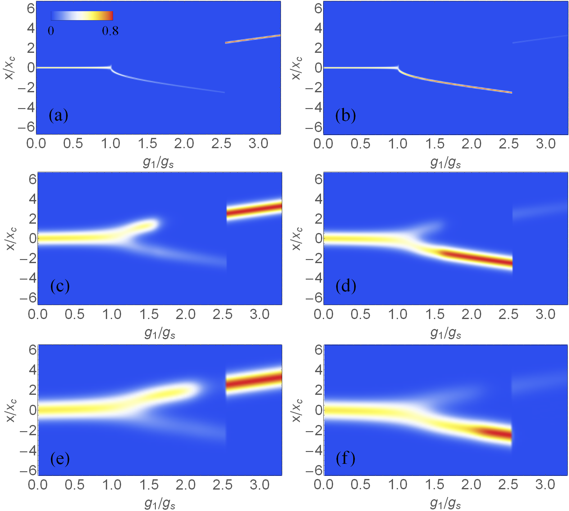
Figure 10: (color online) Wave functions of spin-up (a,c,e) and spin-down (b,d,f) components in phase transitions. (a,b) $\omega=0.001\Omega$, $\epsilon=0.1g_{\mathrm{t}}$. (c,d) $\omega=0.1\Omega$, $\epsilon=0.001g_{\mathrm{t}}$. (e,f) $\omega=0.2\Omega$, $\epsilon=0.0005g_{\mathrm{t}}$. Here we fix $\log[g_{2}/g_{\mathrm{t}}]=-4.5$ and the effective spatial position is scaled by $x_{c}=\sqrt{2}g_{\mathrm{s}}/\omega.$

IX Mechanisms

In this section we should clarify the mechanisms underlying the various patterns of symmetry breaking, the different orders of transitions and the successive transitions in the tricritical picture. To facilitate the understanding we rewrite bosonic mode in the model Hamiltonian in terms of the quantum harmonic oscillator. By the transformation $a^{\dagger}=(\hat{x}-i\hat{p})/\sqrt{2}$, $a=(\hat{x}+i\hat{p})/\sqrt{2}$, we transfer to the space of the effective position $\hat{x}$ and the momentum $\hat{p}$. Thus the Hamiltonian takes the form

$$H=\sum_{\sigma_{z}=\pm}(h^{\sigma_{z}}|\sigma_{z}\rangle\langle\sigma_{z}|+{\frac{\Omega}{2}}|\sigma_{z}\rangle\langle\overline{\sigma}_{z}|)$$ (16)

which is comprised of the effective free-particle part (the $h^{\sigma_{z}}$ term) and tunneling part (the $\Omega$ term). Here $\overline{\sigma}_{z}=-\sigma_{z}$ and $+$ ($-$) labels the up $\uparrow$ (down $\downarrow$) spin. The effective free-particle Hamiltonian in the spin components can be rearranged to be

$$h^{\pm}=\omega\ (\frac{\hat{p}^{2}}{2m_{\pm}}+v_{\pm})+e_{0},\quad v_{\pm}=v_{\pm}^{\mathrm{hp}}+b_{\pm}+b_{0}\mp\epsilon.$$ (17)

where

$$v_{\pm}^{\mathrm{hp}} = \frac{1}{2}m_{\pm}\varpi_{\pm}^{2}[x-x_{0,\pm}]^{2},$$ (18)

$$b_{\pm} = \pm\frac{\widetilde{g}_{2}^{\prime}g_{1}^{\prime 2}}{2(1-\widetilde{g}_{2}^{\prime 2})},$$ (19)

$$b_{0} = -g_{1}^{\prime 2}/[2(1-\widetilde{g}_{2}^{\prime 2})].$$ (20)

We have defined $g_{1}^{\prime}=\sqrt{2}g_{1}/\omega$, $g_{2}^{\prime}=2g_{2}/\omega$ and  $e_{0}=-\omega/2$. Here $m_{\pm}=\left(1\mp g_{2}^{\prime}\pm\chi g_{2}^{\prime}\right)^{-1}$ is the effective mass, $\varpi_{\pm}=[\left(1\pm\chi g_{2}^{\prime}\right)^{2}-g_{2}^{\prime 2}]^{1/2}$ is frequency renormalization. The $x_{0,\pm}=\mp g_{1}^{\prime}/\left(1\mp\widetilde{g}_{2}^{\prime}\right)$ is the potential displacement for the potential minimum shifting horizontally from the origin, while $b_{0}$ is the vertical shift which is both downward for the two spin components. In this picture we see the different roles played by the physical parameters of the model: the linear coupling $g_{1}$ separates the potentials of the two spin components, the bias $\epsilon$ shifts the potentials downwards or upwards oppositely for the two spin components, while the nonlinear interaction $g_{2}$ not only leads to asymmetry in frequency $\varpi_{\pm}$ and potential displacement $x_{0,\pm}$ but also results in vertical potential difference $b_{\pm}.$

IX.1 Semiclassical picture for the various patterns of symmetry breaking

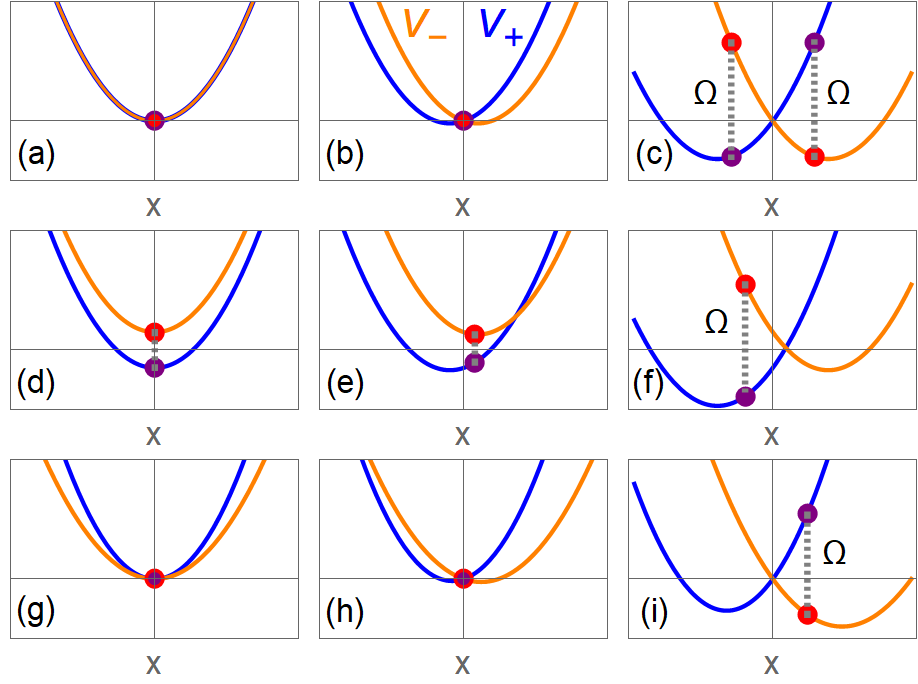
Figure 11: (color online) Semiclassical mechanisms for the different patterns of symmetry breaking. The potentials for spin-up (blue) and spin-down (orange) components for (a-c) $\epsilon=0,g_{2}=0$, (d-f) $\epsilon\neq 0,g_{2}=0$ and (g-i) $g_{2}\neq 0,\epsilon=0$. The linear coupling regimes are (a,d,g) $g_{1}=0$, (b,e,h) $g_{1}<g_{s}$ and (c,f,i) $g_{1}>g_{s}$. The dots mark the effective semi-classical particle positions in the spin-up (purple) and spin-down (Red) potentials.

The phase transitions of the quantum Rabi model occurs at low frequencies. The ground-state wave function basically can be decomposed into ground states of quantum harmonic oscillators with displacement and frequency renormalizations Ying2015 . The wave-packet size is of order $1$ in the afore-presented dimensionless formalism. The potential size at phase transitions can be estimated by $x_{0,\pm},$ being of order $g_{s}^{\prime}=\sqrt{2}g_{s}/\omega\propto\sqrt{\Omega/\omega}$. Thus the ratio between the wave-packet size and the potential size is of order $\sqrt{\omega/\Omega}$ which becomes smaller at a lower frequency. In the low frequency limit, $\omega/\Omega\rightarrow 0$, with the wave-packet size relatively negligible, one can regard the effective particle as a classical mass point, as we have seen in Fig.10(a,b). On the other hand we keep the leading tunneling effect in the spin space. In such a semiclassical consideration, the ground state is motionless with $p\rightarrow 0$, thus the phase transitions and the system properties are decided by the competition of the potential $v_{\pm}$ and the tunneling $\Omega$.

The various patterns of symmetry breaking in the low frequency limit can be readily explained in such semiclassical picture. In Fig. 11, according to different patterns of symmetry breaking we plot the potentials $v_{+}$(blue) for up spin and $v_{-}$(orange) for down spin. The purple (spin up)  and red (spin down) dots mark the positions of the effective mass point and the spin tunneling is indicated by he gray dashed lines.

Fig.11(a-c) present the situation of the conventional quantum Rabi model, in the absence of the bias and the nonlinear interaction. Starting from the zero linear coupling $g_{1}=0$ in panel (a), the spin potentials are identical, with the effective particle staying at the origin where the potential minima are located. The increase of $g_{1}$ separates the potentials horizontally by $x_{0,\pm}$, as indicated in panel (b). However, with a linear coupling below $g_{s}$, the effective particle in the two spin components does not follow the potential separation but remains at the origin instead. This is because moving away from the origin would lose the negative tunneling energy due to the unequal spin weights in the potential difference, while staying at the origin keeps the maximum tunneling energy due to equal spin weights in the degenerate potentials. Increasing $g_{1}$ beyond the critical point, the downward potential shift by $b_{0}$ enlarges the potential difference between the bottom and the origin as in panel (c), so that moving toward the potential bottom will gain more potential energy than the tunneling energy. Therefore the transition occurs and the particle leaves the origin. Note that either before or after the transition the spin distributions are spatially symmetric around the origin and the weights remain equal under spin exchange, thus the parity symmetry is preserved throughout.

Fig.11(d-f) denote the situation of adding a bias to the linear coupling. A bias separates vertically the potentials of the up and down spins at $g_{1}=0$, as in panel (d), which breaks the spin balance and the parity symmetry from the beginning, thus being paramagnetic-like in polarization. In weak linear coupling regime, the bias moves the potential crossing point away from the origin which breaks the space inversion symmetry of the potential. On the other hand, the crossing point is moving to a higher potential which is not energetically favorable. So the parity symmetry is broken in both the spatial and spin parts. In a strong linear coupling beyond the critical point, as in panel (f), any strength of the bias will break the two-side balance maintained by the linear coupling in panel (c), thus a spontaneous symmetry breaking occurs. Note the state on each side is polarized due to the finite difference in spin-up and spin-down energy. Before the spontaneous symmetry breaking, the polarization or spin expectation $\langle\sigma_{z}\rangle$ cancels between the two sides. After the spontaneous symmetry breaking, without the two side cancellation, the polarization jumps to a finite value.

Fig.11(g-i) show the situation of adding a nonlinear interaction to the linear coupling. The nonlinear interaction makes the frequency asymmetric between the up and down spins as in panel (g) and also shifts the spins in vertically opposite directions as in panel (h). However the potential crossing always keeps invariant at the origin. Thus the parity is well preserved even in the presence of a finite nonlinear interaction. Note that the vertical spin-dependent shift $b_{\pm}$ in Eq. (19) has an entangled form of the linear coupling $g_{1}$ and the nonlinear interaction $g_{2}$, increasing the nonlinear interaction at a fixed linear coupling will enlarge the vertical potential difference between the two spin directions. This vertical potential difference will finally surpass the tunneling energy at the origin and lead to symmetry breaking with a first order transition. So the polarization behavior is ferromagnetic-like. In a strong linear coupling beyond the $g_{s}$, also a tiny strength of nonlinear interaction will break the balance on the two sides in panel (c), leading to a spontaneous symmetry breaking from panel (c) to panel (i).

From the basic competitions discussed in the above one can also understand similarly the other mixed patterns of symmetry breaking. For the transition orders we will present some explanations from the view of the variational energy later on in Section IX.3.

IX.2 Scaling of the Stark term

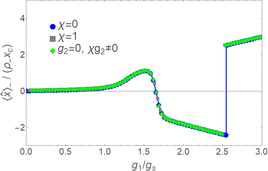
Figure 12: (color online) Scaling of the Stark term. $\langle\hat{x}_{-}\rangle/(\rho_{-}x_{c})$ versus $g_{1}$ with different Stark couplings $\chi=0$ (blue dots), $\chi=1$ (gray squares) and $g_{2}=0,\chi g_{2}\neq 0$ (green diamonds) at a same value of $\widetilde{g}_{2}=(1+\chi)g_{2}$ . Here $\omega=0.1\Omega$, $\epsilon=0.001g_{\mathrm{t}}$ and $\log[\widetilde{g}_{2}/g_{\mathrm{t}}]=-4.5$.

As mentioned around Eq.(2), the properties with the Stark term are similar by included the scaling factor, unless the frequency is high. We illustrate the scaling in Fig.12 where it is shown that different Stark couplings under a fixed value of $\widetilde{g}_{2}=(1+\lambda)g_{2}$ have the same spin expectation and the same successive transition points (around $g_{1}/g_{\mathrm{s}}\sim 1.0,\ 1.6,\ 2.6$). This scaling can be simply understood from the semiclassical picture afore-formulated. In fact, from Eq.(17) we have seen that the potential displacement $x_{0,\pm},$ the effective bias $b_{\pm}$ and and the uniform shift $b_{0}$ are all functions of $\widetilde{g}_{2}^{\prime}=\left(1+\chi\right)g_{2}^{\prime}.$ It should be noted that, although the effective mass $m_{\pm}$ and $\varpi_{\pm}$ respectively are not functions of $\widetilde{g}_{2}^{\prime},$ their joint contribution in $v_{\pm}^{\mathrm{hp}}$ is still a function of $\widetilde{g}_{2}^{\prime}$ as

$$m_{\pm}\varpi_{\pm}^{2}=\frac{[\left(1\pm\chi g_{2}^{\prime}\right)^{2}-g_{2}^{\prime 2}]}{\left(1\mp g_{2}^{\prime}\pm\chi g_{2}^{\prime}\right)}=\left(1\pm\widetilde{g}_{2}^{\prime}\right).$$ (21)

Namely, except for the kinetic term neglected in the semiclassical picture in the low frequency limit, all contributions of the Stark-like term to $v_{\pm}$ can be scaled into a function of $\widetilde{g}_{2}^{\prime}.$ Thus, one will get the same phase diagrams for the presence of the Stark-like term by the scaling factor $\left(1+\chi\right)$.

IX.3 Semiclassical energy competition for the different orders of phase transitions

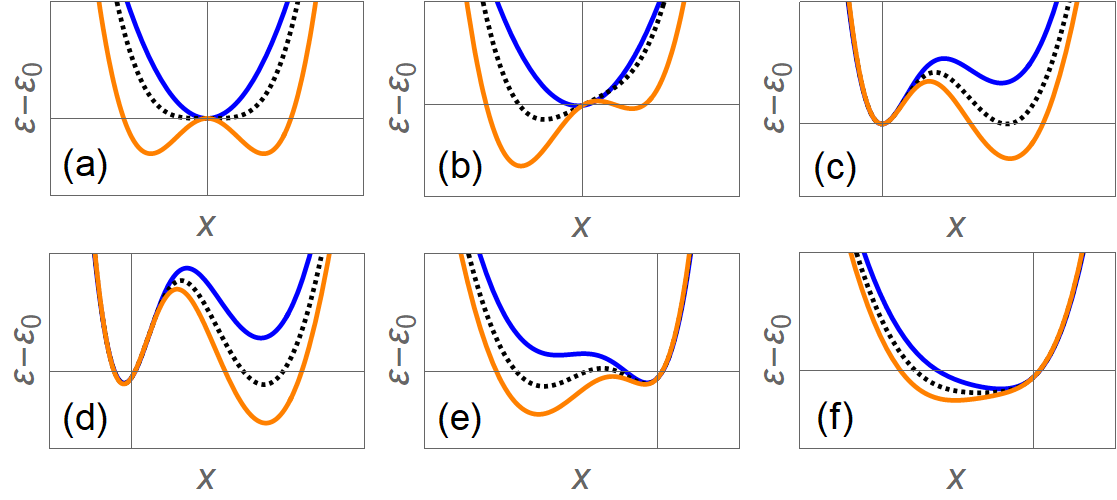
Figure 13: (color online) Energy competitions and transition orders. Semiclassical variational energy $\varepsilon$ before (blue solid lines), at (black dotted lines) and after (orange solid lines) transitions, with respect to the effective particle position $x$ for (a) $\epsilon=0$ and $g_{2}=0$, (b) $\epsilon\neq 0$ and $g_{2}=0$, (c) $\epsilon=0$ and $g_{2}\neq 0$, (d) $\epsilon\neq 0$ and $g_{2}>0$, (e) $\epsilon\neq 0$ and $g_{2}<0$ nearby $g_{2}=g_{t}$, (f) $\epsilon\neq 0$ and $g_{2}<0$ nearby $g_{2}=0$. Here $\varepsilon_{0}=-(\omega+\Omega)/2$.

We can gain more insights from the total energy competition. The variational energy in semiclassical picture can be formulated in the following eigenequation of matrix form

$$\left(\begin{array}[]{cc}\varepsilon_{+}&-\frac{\Omega}{2}\\ -\frac{\Omega}{2}&\varepsilon_{-}\end{array}\right)\left(\begin{array}[]{c}\beta^{+}\\ \alpha^{-}\end{array}\right)=\varepsilon\left(\begin{array}[]{c}\beta^{+}\\ \alpha^{-}\end{array}\right)$$ (22)

where $\varepsilon_{\pm}=\omega\ v_{\pm}+\varepsilon_{0}.$ The eigenenergy for the ground state is determined by

$$\varepsilon=\frac{1}{2}\left[\left(\varepsilon_{+}+\varepsilon_{\_}\right)-\sqrt{\left(\varepsilon_{+}-\varepsilon_{\_}\right)^{2}+\Omega^{2}}\right]$$ (23)

which should be minimized with respect to $x$ as $v_{\pm}$ is position dependent.

In Fig.13 we illustrate the variational energy as a function of $x$ before the transition (blue solid lines), at the transition (black dashed lines) and after the transition (orange solid line) in different situations. Panel (a) presents the case of the conventional quantum Rabi model without the bias and the nonlinear interaction. Before the transition the energy minimum is located at the origin, after the transition the origin becomes an unstable saddle point while the ground state lies in the formed two symmetric minima which are moving away from the origin. At the transition point $g_{1}=g_{\mathrm{s}}$ the minimum bottom becomes flat with a vanishing second derivation $\partial^{2}\varepsilon/\partial x^{2}=0$. Although the transition turns the minimum number from one to two, this transition is continuous as two minimum positions separate continuously from the origin.

The presence of the bias breaks the symmetry in the energy profile in any regime of the linear coupling, as illustrated in Fig.13(b). The profile difference of single minimum and double minimum in energy leads to different response to the bias before and after the transition. Before the transition point $g_{\mathrm{s}}$ the energy has no competition as the single minimum is the only choice. With the bias this single minimum moves gradually away from the origin. After the transition, there are two minima which are degenerate in the absence of the bias. Any tiny strength of bias will immediately break the symmetry and raise the degeneracy. Changing the sign of the bias the ground state will shift from one side of the minimum to the other side. Either the bias opening or sign change will lead to an abrupt jump in polarization, leading to a discontinuous first-order transition.

The scenario of energy competition is different in the presence of nonlinear interaction, as demonstrated in Fig.13(c). There are two local energy minima both before and after the transition (here the transition moves from $g_{\mathrm{s}}$ to $g_{1c}$ in Eq.(3)), one at the origin, the other away from the origin. Before the transition, the ground state lies in the minimum at the origin while the other local minimum is higher in energy. At the transition the higher minimum is lowered to get degenerate with the one at the origin. After the transition, the energy preference gets reversed and the ground state turns to the lower minimum away from the origin. Note that, in a sharp contrast to the continuous variation of the minimum position in panel (a), the transition here in panel (c) is companied with a sudden shift of minimum position. This discontinuous shift of minimum position results in the first-order transition. Conventionally continuous/discontinuous transitions refer to continuity of different-order energy derivatives with the respect to the system parameter, here the continuous/discontinuous variation of minimum position provides another angle of view from the aspect of the variational-energy structure.

In the presence of both the bias and the nonlinear interaction, there are three situations which should be distinguish. Fig.13(d) shows the first case in which the bias $\epsilon$ and the nonlinear interaction $g_{2}$ have the the same sign. In his case the bias pushes the minimum at the origin away to the opposite side of the higher minimum. In this case the transition also is discontinuous, similar to panel (c), which accounts for the first-order boundary in the positive-$g_{2}$ regime of Fig. 2(d). This first order transition boundary covers all range of the linear coupling $g_{1}$. Fig.13(e) shows the second case with the sign of $g_{2}$ opposite to $\epsilon$ and the amplitude of $g_{2}$ closer to $g_{\mathrm{t}}$. In this case the two energy minima are located on the same side but still far away enough to have a barrier between them. Thus the transition also has a discontinuous shift of the minimum position, which corresponds to the first-order boundary arc in the negative-$g_{2}$ regime of Fig. 2(d). The third situation shown in Fig.13(f) still has opposite signs of $g_{2}$ and $\epsilon$ but with a small amplitude of $g_{2}$. In this case the two local energy minima are too close to have a barrier to separate them explicitly. Although the minimum position may have a quick shift but the variation is continuous. Thus the first order transition is softened, being second-order like or even fading away. This corresponds to the regime above the arc boundary in Fig. 2(d) where the first-order boundary disappears.

IX.4 Full-quantum-mechanical effect for the novel successive transitions and tricriticalities

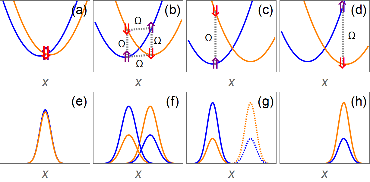
Figure 14: (color online) Full-quantum-mechanical mechanisms for additional transition in successive transitions. (a-d) Effective potentials for the spin-up (blue) and spin-down (orange) components, the arrows represents the spins and gray dashed lines denotes the tunneling channels. (e-h) Schematic decomposed wave functions in the spin-up (blue) and spin-down (orange) components. The dashed lines in (g) show the vanishing left-right wave-packet overlap and indicate the disappearing wave packets.

In the afore-discussed semiclassical picture there is no spatial structure of wave function or probability distribution over the effective spatial space. This simplification will miss some physics that becomes important at finite frequencies. Indeed, as described in Section VI, the novel successive transitions and tricriticalities emerge at a finite frequencies, which cannot be captured by the semiclassical picture. To understand these novel phenomena we shall fall back on a full-quantum-mechanical picture. To include all the quantum states in one example we follow the wave function evolution in Fig.10(c,d) where there are four quantum states. Accordingly, in Fig. 14, we sketch the spin potentials (upper panels) and the wave-function profiles (lower panels). The wave function is decomposed into left and right wave packets, as analyzed in a polaron-antipolaron picture Ying2015 , due to the barrier indicated in Fig.13. Each wave packet is represented by a displaced ground state of quantum harmonic oscillator Ying2015 ; Bera2014Polaron and the heights indicate the weights.

There are three transitions in the illustrated case, going through transitions I, III and IV in Fig.7(e,f). Before the first transition, the tunneling energy is dominating. As in Fig.14(a,e), the single wave packets in both spins reside around the origin where the potential crossing point is located. The degeneracy at the crossing point yield equal weights of the two spin components. Both the single-wave-packet profiles and equal spin weights help to gain a maximum tunneling energy. The equal spin-component weight and the full overlapping yield a vanishing spin expectation $\langle\sigma_{z}\rangle$ and a saturation of $\langle\sigma_{x}\rangle.$

Transition-I:  Increasing the linear coupling separates the potentials more and lower the potential bottoms, so that the potential energy comes to compete with the tunneling energy. After the first transition, as in Fig. 14(b,f), the wave function splits into four wave packets. Differently from the semiclassical picture there are now four channels of tunneling. The left-right tunneling arises due to the left-right overlaps of the wave packets, while the semiclassical particle has no such left-right overlap in any case. These left-right tunneling channels come to play an important role to balance potential asymmetry caused by the bias or the nonlinear interaction. Note in such a four-channel state, the polarizations of the two sides are canceling each other so that $\langle\sigma_{z}\rangle$ still remains almost vanishing at the presence of a weak bias and nonlinear interaction. Therefore, $\langle\sigma_{z}\rangle$ does not have an obvious change across the first transition thus the first transition leaves little imprint in $\langle\sigma_{z}\rangle$. On the other hand, the separated wave packets are moving away from the origin, the potential difference leads to unequal weights of the two spin components on each side. This weight difference lead to the reduction of spin flipping amplitude thus $\langle\sigma_{x}\rangle$ is decreasing in strength. As a result, $\langle\sigma_{x}\rangle$ is sensitive to the first transition and exhibits a critical behavior of second-order transition.

Transition-III: Further increase of $g_{1}$ will separate the wave packets more so that the left-right overlap becomes vanishing, as indicated in Fig. 14(g). Thus the left-right channels of tunneling in a vanishing strength cannot balance the potential asymmetry any more. As a result, the wave packets on the higher-potential side disappear and the second transition occurs. Note that at a higher frequency would have wider wave packets, thus the left-right overlap survive till larger $g_{1}$ and the transition occurs later. After this transition, the left-right cancellation does not exist in the one-side state so that $\langle\sigma_{z}\rangle$ jumps from a vanishing value to a finite value. Consequently this transition can find a clear signal in $\langle\sigma_{z}\rangle$.  On the other hand, the state on the two sides have a similar amplitude of difference in the weights for the spin components. Note the strength of $\langle\sigma_{x}\rangle$ is decided by the weight difference of the two spins no matter which spin component has more weight. Thus $\langle\sigma_{x}\rangle$ does not respond to this transition unless the potential asymmetry is large in the presence of strong bias and nonlinear interaction. Transition II has the same nature as transition III, although not present in the example of Fig.14.

Transition-IV: An even larger $g_{1}$ will enhance much the entangled effective bias $b_{\pm}$ which is proportional to $g_{1}^{2}$. This enhanced bias will surpass the system bias $\epsilon$ which is originally stronger in small-$g_{1}$ regime. This strength reversion of the two competing biases triggers transition IV. In principle, at the reversion the system should return to the four-wavepacket state. However the left-right overlap is too small to maintain four-wavepacket state long enough to open a phase, unless the frequency is higher to get more-broadened wave packets. Hence, transition IV simply appears as one sharp transition. At a higher frequency the wave packets could be more more-broadened so that some left-right overlap could still remain, in such a situation Transition-IV could be bifurcated into two close transitions as mentioned for the tendency of four successive transitions in Section VI.6. Since the state shifts from one side to the other, the sign of $\langle\sigma_{z}\rangle$ get reversed so that $\langle\sigma_{z}\rangle$ exhibits a first-order change at this transition. In the same reason as in Transition-III $\langle\sigma_{x}\rangle$ still shows no sign at Transition-IV.

From the above understanding we see that $\langle\sigma_{x}\rangle$ can be sensitive to measure the first transition and $\langle\sigma_{z}\rangle$ is useful to track all the other transitions. The spin-filtered quantity $\langle{a^{{\dagger}}+a\rangle}_{\pm}/\rho_{\pm}$ is the spin displacement in our picture, i.e, the effective wave-packet position in each spin component. So it is naturally sensitive to the side shifting in transitions II,III,IV. Moreover, in the four-wavepacket state after transition I, each spin component has imbalanced weights of the left-side wave packet and the right-side wave packet, due to the potential difference within $v_{+}$ or $v_{-}$ as shown in Fig.14(b). Indeed $\langle{a^{{\dagger}}+a\rangle}_{\pm}/\rho_{\pm}$ reflects the effective mass center of each spin component, which is moving away from the origin after transition I. In consequence, $\langle{a^{{\dagger}}+a\rangle}_{\pm}/\rho_{\pm}$ is also responding to transition I, thus useful to detect all transitions simultaneously.

X Finding analytic boundaries

In previous sections IV-VII we have given the analytic phase boundaries in the description of the phase diagrams. In Sections VIII and IX we have got a basic understanding of the different transitions from the wave function changeovers and energy competitions. This would facilitate the finding of analytic boundaries. Now we try to provide some brief derivations for the analytic phase boundaries.

X.1 Analytic boundaries in low frequency limit

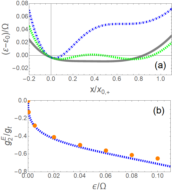
Figure 15: (color online) Saddle point flattening and ending points of the arc boundary. (a) Semiclassical variational energy at the end of the arc boundary $g_{1}=0.763g_{\mathrm{s}}$, $g_{2}=-0.554g_{\mathrm{t}}$(gray solid), in the arc $g_{1}=0.7g_{\mathrm{s}}$, $g_{2}=-0.665g_{\mathrm{t}}$ (green dashed) and at an infection point $g_{1}=0.5g_{\mathrm{s}}$, $g_{2}=-0.81g_{\mathrm{t}}$ (blue dot-dashed). Here $\epsilon=10g_{\mathrm{t}}$ and $\omega=0.001\Omega$. (b) Critical value $g_{2}^{\mathrm{E}}$ at the end of the arc boundary versus the bias $\epsilon$ from numerics (dots) and the analytic result (blue dashed).

With the clarifications of the mechanisms for all the transitions, we can extract the analytic phase boundaries. In the low frequency limit, the boundary can be obtained from the semiclassical picture. The energy minima can be available by minimization of the variational energy $\varepsilon$ with respect to the position,

$$\frac{\partial}{\partial x}\varepsilon\left(x\right)=0$$ (24)

which gives three roots $x_{\mathrm{R}}$, $x_{\mathrm{S}}$, $x_{\mathrm{L}}$. The root $x_{\mathrm{S}}$ between the other two $x_{\mathrm{R}}$, $x_{\mathrm{L}}$ is the saddle point. The transition boundary is then decided by

$$\varepsilon\left(x_{\mathrm{R}}\right)=\varepsilon\left(x_{\mathrm{L}}\right)$$ (25)

which leads us to

$$\left|g_{1c}\right|=g_{\mathrm{s}}[1+\frac{g_{\mathrm{t}}\epsilon}{\widetilde{g}_{2}\Omega}]\sqrt{1-\widetilde{g}_{2}^{2}/g_{\mathrm{t}}^{2}}$$ (26)

in Eqs. (4) and (5).

Note that, as mentioned for Fig. 2 (d), in the regime of negative $g_{2}$, the above boundary (26) is an arc. Along this arc boundary the transition is of first order. At the ends of the arc the transition becomes second order and boundary closes. As revealed in Section IX.3, the first-order transition arises from the energy saddle point $x_{\mathrm{S}}$ which separates two competing minima. Disappearing of the energy saddle will mean fading away of the first-order transition. The critical point comes with a flattened saddle. We show this saddle flattening in Fig. 15(a). Here, the green dashed line illustrates the minimum-saddle-minimum of the variational energy $\varepsilon$ at a point along the first-order boundary, while the gray solid line shows the situation at the ends of the boundary where a flattened bottom can be clearly seen. This critical point can be figured out by vanishing of the first and second derivatives of the variational energy

$$\frac{\partial\varepsilon\left(x\right)}{\partial x}=0,\quad\frac{\partial^{2}\varepsilon\left(x\right)}{\partial x^{2}}=0.$$ (27)

It should be mentioned (27) is a necessary condition but not a sufficient one. We give an example by the blue dot-dashed line in Fig. 15(a), where the middle point of the shoulder shape fulfils (27) but it is an inflection point instead of a saddle point. Nevertheless, we can combine condition (27) and boundary (26) to extract the critical point,

$$g_{2}^{\mathrm{E}}\approx 3\left(\frac{\epsilon}{5\Omega}\right)^{1/3}+\frac{226\epsilon}{75\Omega}-\frac{362011}{27000}\left(\frac{\epsilon}{5\Omega}\right)^{5/3},$$ (28)

approximately for a weak bias and a non-linear interaction. Fig.15(b) shows the above analytic $g_{2}^{\mathrm{E}}$ (dashed line) in comparison with the numerical ones (dots). It is interesting to see in the weak-bias regime $g_{2}^{\mathrm{E}}$ is in a fractional power law, which means $g_{2}^{\mathrm{E}}$ increases quickly with a small strength of the bias. A small bias could break and open much the ring of the round boundary in Fig. 2.

X.2 Analytic boundaries for the successive transitions at finite frequencies

Based on the physical picture analyzed in Section IX.4 we can obtain the phase boundaries in the tricritical scenarios at finite frequencies. Unlike in the semiclassical picture, now the left and right states can simultaneously get involved in a ground state. We also decompose the wave function into right (R) and left (L) states $\left|\Psi\right\rangle=c_{\mathrm{R}}\left|\psi_{\mathrm{R}}\right\rangle+c_{\mathrm{L}}\left|\psi_{\mathrm{L}}\right\rangle$ upto a normalization factor. The right/left states are respectively formed in the same-side tunneling $\Omega_{\alpha\beta}$ and $\Omega_{\alpha\beta}$

$$\left|\psi_{\mathrm{L}}\right\rangle = \alpha^{+}\varphi_{\alpha}^{+}\left|\uparrow\right\rangle+\beta^{-}\varphi_{\beta}^{-}\left|\downarrow\right\rangle,$$ (29)

$$\left|\psi_{\mathrm{R}}\right\rangle = \alpha^{-}\varphi_{\alpha}^{-}\left|\downarrow\right\rangle+\beta^{+}\varphi_{\beta}^{+}\left|\uparrow\right\rangle,$$ (30)

where $\alpha^{\pm},\beta^{\pm}$ represent the weight of the wave packet $\varphi_{j}^{\pm}$. The corresponding energy can be easily obtained as

$$\varepsilon_{\mathrm{L}} = \frac{1}{2}\left[(h_{\beta\beta}^{-}+h_{\alpha\alpha}^{+})-\sqrt{(h_{\beta\beta}^{-}-h_{\alpha\alpha}^{+})^{2}+S_{\alpha\overline{\beta}}^{2}\Omega^{2}}\right],$$ (31)

$$\varepsilon_{\mathrm{R}} = \frac{1}{2}\left[(h_{\beta\beta}^{+}+h_{\alpha\alpha}^{-})-\sqrt{(h_{\beta\beta}^{+}-h_{\alpha\alpha}^{-})^{2}+S_{\beta\overline{\alpha}}^{2}\Omega^{2}}\right].$$ (32)

Here we define $h_{ij}^{\pm}=\langle\varphi_{\mathrm{i}}^{\pm}|\left(h^{\pm}-b_{0}-\varepsilon_{0}\right)|\varphi_{\mathrm{j}}^{\pm}\rangle$, where the irrelevant constants $b_{0}$ and $\varepsilon_{0}$ have been substracted, and $S_{i\overline{j}}=\langle\varphi_{\mathrm{i}}^{+}|\varphi_{\mathrm{j}}^{-}\rangle$ is the wave-packet overlap. The wave packet $\varphi_{\mathrm{j}}^{\pm}$ can be well approximated by the displaced ground state of quantum harmonic oscillator, with the displacement $\zeta_{i,\pm}x_{0,\pm}$ renormalized from the position of the potential bottom $x_{0,\pm}$Ying2015 . Explicitly we have

$$h_{ii}^{\pm}=\frac{\omega}{2}\left\{\varpi_{\pm}-\frac{[1-(1-\zeta_{i,\pm})^{2}]g_{1}^{\prime 2}}{(1\pm\widetilde{g}_{2}^{\prime})}\right\}\mp\epsilon,$$

and $S_{\alpha\overline{\beta}}\approx S_{\beta\overline{\alpha}}\approx 1$ in gaining the maximum tunneling energy. The successive transitions occur in weak bias and nonlinear interaction, in such situations we keep the leading order

$$\varepsilon_{\mathrm{L}}-\varepsilon_{\mathrm{R}}=\overline{g}_{2}\overline{g}_{1}^{2}\zeta^{2}\left[\frac{\left(1+\zeta/2\right)}{\sqrt{(\zeta^{2}+\overline{g}_{1}^{-4})}}-1\right]\Omega-\frac{2\zeta\epsilon}{\sqrt{(\zeta^{2}+\overline{g}_{1}^{-4})}},$$ (33)

with $\zeta=(1-\overline{g}_{1}^{-4})^{1/2}$ being the displacement renormalization from the conventional QRM Ying2015 .

Standing in a phase of the two-branch state, we can judge the onset of the transitions to other states by an exponential decay of the state weight on one side, $\delta_{c}=\left(c_{\mathrm{R}}/c_{\mathrm{L}}\right)^{\pm 1}\sim e^{-1}$, where $\pm 1$ depends on which broken-branch state the system is transiting to. Thus at the transition we can treat by a perturbation from the left-right tunneling energy ($\Omega_{\alpha\alpha}$, $\Omega_{\beta\beta})$ as well as the single-particle left-right overlap energy ($t_{\alpha\beta}^{+},t_{\beta\alpha}^{-})$

$$\delta_{c}=(\Omega_{\alpha\alpha}+\Omega_{\beta\beta}+t_{\alpha\beta}^{+}+t_{\beta\alpha}^{-})/\left[\eta_{\mathrm{LR}}\left(\varepsilon_{\mathrm{L}}-\varepsilon_{\mathrm{R}}\right)\right],$$ (34)

where $\eta_{\mathrm{LR}}=\pm 1$ is decided by which side of state has a lower energy. In the leading order, we have

$$\Omega_{\alpha\alpha}+\Omega_{\beta\beta} \approx -\frac{\Omega}{2}S_{\alpha\overline{\alpha}},$$ (35)

$$t_{\alpha\beta}^{+}+t_{\beta\alpha}^{-} \approx \alpha\beta\left[\omega+\left(1-\zeta\right)^{2}\overline{g}_{1}^{2}\frac{\Omega}{2}\right]S_{\alpha\beta},$$ (36)

where $\alpha=\sqrt{\left(1+\zeta\right)/2}$ and $\beta=\sqrt{\left(1-\zeta\right)/2}$ from the conventional QRM Ying2015 are the leading contributions for $\alpha^{\pm},\beta^{\pm}$ which get involved via $t_{ij}^{\pm}=w_{ij}h_{ij}^{\pm}$ , with $w_{ij}$ being the weight product of $\alpha^{\pm}$ and $\beta^{\pm}.$ $S_{\alpha\beta}\approx S_{\alpha\overline{\alpha}}\approx\exp[-\zeta^{2}\overline{g}_{1}^{2}\Omega/(2\omega)]$ is approximate left-right wavepacket overlap.

Combining (33) and (34), we get analytic expressions for boundaries II and III

$$\widetilde{g}_{2c}^{\mathrm{II,III}}=\pm\frac{(1-t)g_{\mathrm{t}}}{\delta_{c}\zeta^{3}\overline{g}_{1}^{2}}\exp[-\frac{\zeta^{2}\overline{g}_{1}^{2}\Omega}{2\omega}]+\frac{4\epsilon}{\zeta^{2}\overline{g}_{1}^{2}\Omega}g_{\mathrm{t}}.$$ (37)

Transition-IV is the shifting between pure left state and pure right state, thus setting $\varepsilon_{\mathrm{L}}-\varepsilon_{\mathrm{R}}=0$ we find

$$\widetilde{g}_{2c}^{\mathrm{IV}}=\frac{4\epsilon}{\zeta^{2}\overline{g}_{1}^{2}\Omega}g_{\mathrm{t}}+O[\left(\frac{\epsilon}{\Omega}\right)^{3}].$$ (38)

As we have seen from Figs. 4,5,7,8,9 in Section VI, these analytic boundaries work quite well in comparison with the numerics.

XI Conclusions and discussions

By combining exact diagonalization and analytic methods in a semiclassical picture and a full quantum-mechanical picture, we have presented a thorough study on the ground state of the quantum Rabi model in the presence of the bias and the nonlinear interaction. The model exhibits different patterns of symmetry breaking, including the paramagnetic-like, antiferromagnetic like, spontaneous symmetry breaking, paramagnetic-like plus first/second-order transitions, antiferromagnetic-like plus first/second-order transitions. These symmetry-breaking patterns bring a rich and colorful world of phase diagrams. We have obtained the full phase diagrams and the analytic phase boundaries, both in the low frequency limit and at finite frequencies. Five different situations for the occurrence of tricriticality are unveiled, respectively: (i) induced by the competition of the linear coupling and nonlinear interaction in the presence of the bias, in the low frequency limit. (ii) induced by raising the frequency in the respective presence of the nonlinear interaction or the bias. (iii) induced by the competition of linear coupling with the nonlinear interaction or the bias, under fixed finite frequencies. (iv) induced by the interplay of linear coupling with both the nonlinear interaction and the bias, under fixed finite frequencies. (iv) induced by varying the frequency in the interplay of the nonlinear interaction and the bias. The system could have four different quantum phases, we revealed that all four phases can meet to form quadruple points. The low-frequency-limit phase boundary of nonlinear interaction in the absence of bias turns out to be a quadruple line. In comparison with the semiclassical low-frequency limit, the finite frequencies lead to more phase transitions. By analyzing the energy competitions and monitoring the essential changes of quantum states in the transitions, we have clarified the semiclassical and quantum-mechanical mechanisms underlying the afore-mentioned phenomena. We see that the full quantum-mechanical effect leads to much richer physics than the semiclassical picture, including additional phase transitions, novel tricriticalities, and formation of quadruple points as well as a fine structure of spontaneous symmetry breaking.

Note that the model we consider can be implemented in the experimental setups as in the superconducting circuit systemFelicetti2018-mixed-TPP-SPP ; Bertet-Nonlinear-Experim-Model-2005 . It is convenient to cool the superconducting circuits down to the ground state. On the other hand, the model parameters are controllable as the superconducting systems are composed of LC circuits of which the frequency parameters are quite tunable. It is worthwhile to give an estimation on the regime of experimental parameters that is favorable for detections of the phenomena we address in the present work, such as successive transitions and tricricalities. The symmetry breaking patterns, second/first-order transitions and tricriticality-(i) in the low frequency limit are illustrated at frequencies of order $\omega=0.001\sim 0.01\Omega$, while the nonlinear interaction $g_{2}$ has an order similar to $\omega$ and the bias is in a range of order around $\epsilon=0\sim 10\omega.$ A typical experimental strength for the tunneling strength $\Omega$ is of order $10$GHz Blais-2004-exp-parameters in superconducting circuit systems, although the order can reach $50$GHz in microwave cavities and even $350$THz in optical cavities. For the superconducting systems we are more concerned, the frequency $\omega=0.001\sim 0.01\Omega$ corresponds to the order $10\sim 100$MHz. The additional transitions and the novel tricricalities occur at the finite frequencies of order around $\omega=0.1\Omega\sim 1\Omega$, while $\epsilon$ and $g_{2}$ are illustrated in a range of $10^{-5}\sim 10^{-1}g_{\mathrm{t}}$ where $g_{\mathrm{t}}$ is of the same order of $\omega$. In LC circuits these parameters would correspond to $\omega=1\sim 10$GHz and $\epsilon,g_{2}=10^{-2}\sim 10^{3}$MHz. These parameter regimes would open a wide window accessible for the circuit systems.

Our results would be relevant for the growing interest in the nonlinear effectYing-2018-arxiv ; Felicetti2015-TwoPhotonProcess ; Puebla2017-TwoPhotonProcess ; Felicetti2018-mixed-TPP-SPP ; Bertet-Nonlinear-Experim-Model-2005 ; Casanova2018npj ; Puebla2019 ; CongLei2019 ; Xie2019 ; ZhengHang2017 ; PengJie2019 ; FelicettiPRL2020 in the context of continuing enhancements of experimental light-matter couplingsDiaz2019RevModPhy ; Wallraff2004 ; Gunter2009 ; Niemczyk2010 ; Peropadre2010 ; FornDiaz2017 ; Forn-Diaz2010 ; Scalari2012 ; Xiang2013 ; Yoshihara2017NatPhys ; Yoshihara2017 ; Kockum2017 . Our analytic phase boundaries and physical analysis may provide some convenience and insights. We speculate that the phenomena revealed here on the classical-to-quantum transition and nonlinearity might also leave imprints in the Bloch-Siegert effectPietikainen2017 and dynamicsWolf2012 ; Hwang2015PRL ; Crespi2012 , which we shall discuss in some other works.

References

- (1) P. Forn-Díaz, L. Lamata, E. Rico, J. Kono, and E. Solano, Rev. Mod. Phys. 91, 025005 (2019) and references therein.
- (2) D. Braak, Phys. Rev. Lett. 107, 100401 (2011).
- (3) A. Le Boité, Adv. Quantum Technol. 3, 1900140 (2020).
- (4) A. Frisk Kockum, A. Miranowicz, S. De Liberato, S. Savasta, and F. Nori, Nature Reviews Physics 1, 19 (2019).
- (5) E. T. Jaynes and F. W. Cummings, Proc. IEEE 51, 89 (1963).
- (6) I. I. Rabi, Phys. Rev. 51, 652 (1937).
- (7) G. Romero, D. Ballester, Y. M. Wang, V. Scarani, and E. Solano, Phys. Rev. Lett. 108, 120501 (2012).
- (8) J. S. Pedernales, M. Beau, S. M. Pittman, I. L. Egusquiza, L. Lamata, E. Solano, and A. del Campo, Phys. Rev. Lett. 120, 160403 (2018).
- (9) F. A. Wolf, M. Kollar, and D. Braak, Phys. Rev. A 85, 053817 (2012).
- (10) E. Solano, Physics 4, 68 (2011).
- (11) Q.-H. Chen, C. Wang, S. He, T. Liu, and K.-L. Wang, Phys. Rev. A 86, 023822 (2012).
- (12) Q.-T. Xie, S. Cui, J.-P. Cao, L. Amico, and H. Fan, Phys. Rev. X 4, 021046 (2014).
- (13) E. K. Irish and J. Gea-Banacloche, Phys. Rev. B 89, 085421 (2014).
- (14) M. T. Batchelor and H.-Q. Zhou Phys. Rev. A 91, 053808 (2015).
- (15) S. Ashhab, Phys. Rev. A 87, 013826 (2013).
- (16) M.-J. Hwang, R. Puebla, and M. B. Plenio, Phys. Rev. Lett. 115, 180404 (2015).
- (17) Z.-J. Ying, M. Liu, H.-G. Luo, H.-Q.Lin and J. Q. You, Phys. Rev. A 92, 053823 (2015).
- (18) M. Liu, S. Chesi, Z.-J. Ying, X. Chen, H.-G. Luo, and H.-Q. Lin, Phys. Rev. Lett. 119, 220601 (2017).
- (19) L. Cong, X.-M. Sun, M. Liu, Z.-J. Ying, and H.-G. Luo, Phys. Rev. A 95, 063803 (2017).
- (20) Z.-J. Ying, L. Cong, and X.-M. Sun, arXiv:1804.08128, J. Phys. A: Math. Theor. 53, 345301 (2020).
- (21) M. Liu, Z.-J. Ying, J.-H. An, and H.-G. Luo, New J. Phys. 17, 043001 (2015).
- (22) M. Liu, Z.-J. Ying, J.-H. An, H.-G. Luo and H.-Q. Lin, J. Phys. A: Math. Theor. 50, 084003 (2017).
- (23) L. Cong, X.-M. Sun, M. Liu, Z.-J. Ying, and H.-G. Luo Phys. Rev. A 99, 013815 (2019).
- (24) L. Yu, S. Zhu, Q. Liang, G. Chen, and S. Jia, Phys. Rev. A 86, 015803 (2012).
- (25) Y. Wang, W.-L. You, M. Liu, Y.-L. Dong, H.-G. Luo, G. Romero, and J. Q. You, New J. Phys. 20, 053061 (2018).
- (26) T. Liu, M. Feng, W. L. Yang, J. H. Zou, L. Li, Y. X. Fan, and K. L. Wang, Phys. Rev. A 88, 013820 (2013).
- (27) Y.-Y. Zhang, Phys. Rev. A 94, 063824 (2016).
- (28) L.-T. Shen, Z.-B. Yang, H.-Z. Wu, and S.-B. Zheng, Phys. Rev. A 95, 013819 (2017).
- (29) F. H. Maldonado-Villamizar, C. H. Alderete, and B. M. Rodríguez-Lara, Phys. Rev. A 100, 013811 (2019).
- (30) L. Cong, S. Felicetti, J. Casanova, L. Lamata, E. Solano, and I. Arrazola, Phys. Rev. A 101, 032350 (2020).
- (31) Q. Xie, H. Zhong, M. T. Batchelor, and C. Lee, J. Phys. A: Math. Theor. 50, 113001 (2017).
- (32) H. Zhong, Q. Xie, M. T. Batchelor, and C. Lee, J. Phys. A: Math. Theor. 46, 415302 (2013).
- (33) H. P. Eckle and H. Johannesson, J. Phys. A: Math. Theor. 50, 294004 (2017).
- (34) V. Penna, F. A. Raffa, and R. Franzosi, J. Phys. A: Math. Theor. 51, 045301 (2018).
- (35) A. J. Maciejewski and T. Stachowiak, J. Phys. A: Math. Theor. 52, 485303 (2019).
- (36) Y.-F. Xie, L.-W. Duan, and Q.-H. Chen, J. Phys. A: Math. Theor. 52, 245304 (2019).
- (37) A. Wallraff, D. I. Schuster, A. Blais, L. Frunzio, R.-S. Huang, J. Majer, S. Kumar, S. M. Girvin, and R. J. Schoelkopf, Nature 431, 162 (2004).
- (38) T. Niemczyk, F. Deppe, H. Huebl, E. P. Menzel, F. Hocke, M. J. Schwarz, J. J. Garcia-Ripoll, D. Zueco, T. Hümmer, E. Solano, A. Marx, and R. Gross, Nature Phys. 6, 772 (2010).
- (39) G. Günter, A. A. Anappara, J. Hees, A. Sell, G. Biasiol, L. Sorba, S. De Liberato, C. Ciuti, A. Tredicucci, A. Leitenstorfer and R. Huber, Nature 458, 178 (2009).
- (40) P. Forn-Díaz, J. J. García-Ripoll, B. Peropadre, J. L. Orgiazzi, M. A. Yurtalan, R. Belyansky, C.M. Wilson, and A. Lupascu, Nat. Phys. 13, 39 (2017).
- (41) B. Peropadre, P. Forn-Díaz, E. Solano, and J. J. García-Ripoll, Phys. Rev. Lett. 105, 023601 (2010).
- (42) P. Forn-Díaz, J. Lisenfeld, D. Marcos, J. J. Garcia-Ripoll, E. Solano, C. J. P. M. Harmans, and J. E. Mooij, Phy.Rev. Lett. 105, 237001 (2010).
- (43) G. Scalari, C. Maissen, D. Turčinková, D. Hagenmüller, S. De Liberato, C. Ciuti, C. Reichl, D. Schuh, W. Wegscheider, M. Beck, and J. Faist, Science 335, 1323 (2012).
- (44) Z.-L. Xiang, S. Ashhab, J. Q. You, and F. Nori, Rev. Mod. Phys. 85, 623 (2013).
- (45) F. Yoshihara, T. Fuse, S. Ashhab, K. Kakuyanagi, S. Saito, and K. Semba, Nat. Phys. 13, 44 (2017).
- (46) F. Yoshihara, T. Fuse, S. Ashhab, K. Kakuyanagi, S. Saito, and K. Semba, Phys. Rev. A 95, 053824 (2017).
- (47) X. Gu, A. F. Kockum, A. Miranowicz, Y. X. Liu, F. Nori, Phys. Rep. 718, 1 (2017).
- (48) S. Ashhab and F. Nori, Phys. Rev. A 81, 042311 (2010).
- (49) S. Felicetti, D. Z. Rossatto, E. Rico, E. Solano, and P. Forn-Díaz, Phys. Rev. A 97, 013851 (2018).
- (50) S. Felicetti, J. S. Pedernales, I. L. Egusquiza, G. Romero, L. Lamata, D. Braak, and E. Solano, Phys. Rev. A 92, 033817 (2015).
- (51) R. Puebla, M.-J. Hwang, J. Casanova, and M. B. Plenio, Phys. Rev. A 95, 063844 (2017).
- (52) S. Felicetti,M.-J. Hwang, and A. Le Boité, Phy. Rev. A 98, 053859 (2018).
- (53) I. Travnec, Phys. Rev. A 85, 043805 (2012); A. J. Maciejewski, M. Przybylska, and T. Stachowiak, ibid. 91, 037801 (2015); I. Travnec, ibid. 91, 037802 (2015).
- (54) C. F. Lo, K. L. Liu, and K. M. Ng, EPL (Europhysics Letters) 42, 1 (1998).
- (55) L. Duan, Y.-F. Xie, D. Braak, and Q.-H. Chen, J. Phys. A 49, 464002 (2016).
- (56) L. Garbe, I. L. Egusquiza, E. Solano, C. Ciuti, T. Coudreau, P. Milman, and S. Felicetti, Phys. Rev. A 95, 053854 (2017).
- (57) J. Casanova, R. Puebla, H. Moya-Cessa and M. B. Plenio, npj Quantum Information 4, 47 (2018).
- (58) Y.-F. Xie, L. Duan, and Q.-H. Chen, Phys. Rev. A 99, 013809 (2019).
- (59) J. Peng, E. Rico, J. Zhong, E. Solano, and I. L. Egusquiza Phys. Rev. A 100, 063820 (2019).
- (60) S. Felicetti and A. Le Boité, Phys. Rev. Lett. 124, 040404 (2020).
- (61) P. Bertet, I. Chiorescu, C. J. P. M. Harmans, and J. E. Mooij, arXiv:cond-mat/0507290.
- (62) P. Bertet, I. Chiorescu, G. Burkard, K. Semba, C. J. P. M. Harmans, D. P. DiVincenzo, and J. E. Mooij, Phys. Rev. Lett. 95, 257002 (2005).
- (63) J. E. Mooij, T. P. Orlando, L. Levitov, L. Tian, C. H. van der Wal, S. Lloyd, Science 285, 1036 (1999).
- (64) S. Bera, S. Florens, H. U. Baranger, N. Roch, A. Nazir, and A. W. Chin, Phys. Rev. B 89, 121108(R) (2014).
- (65) A. Blais, R.-S. Huang, A. Wallraff, S. M. Girvin, and R. J. Schoelkopf, Phys. Rev. A 69, 062320 (2004).
- (66) R. Puebla, J. Casanova, O. Houhou, E. Solano, and M. Paternostro, Phys. Rev. A 99, 032303 (2019).
- (67) Z. Lü, C. Zhao, and H. Zheng, J. Phys. A: Math. Theor. 50, 074002 (2017).
- (68) I. Pietikäinen, S. Danilin, K. S. Kumar, A. Vepsäläinen, D. S. Golubev, J. Tuorila, and G. S. Paraoanu, Phys. Rev. B 96, 020501(R) (2017).
- (69) A. Crespi, S. Longhi, and R. Osellame, Phys. Rev. Lett. 108, 163601 (2012).