Length scale dependent elasticity in DNA from coarse-grained and all-atom models

Abstract

The mechanical properties of DNA are typically described by elastic theories with purely local couplings (on-site models). We discuss and analyze coarse-grained (oxDNA) and all-atom simulations, which indicate that in DNA distal sites are coupled. Hence, off-site models provide a more realistic description of the mechanics of the double helix. We show that off-site interactions are responsible for a length scale dependence of the elasticity, and we develop an analytical framework to estimate bending and torsional persistence lengths in models including these interactions. Our simulations indicate that off-site couplings are particularly strong for certain degrees of freedom, while they are very weak for others. If stiffness parameters obtained from DNA data are used, the theory predicts large length scale dependent effects for torsional fluctuations and a modest effect in bending fluctuations, which is in agreement with experiments.

I Introduction

Mechanical properties of DNA strongly influence how the double helix performs its various tasks in the cell, where it is often bent and twisted Aggarwal et al. (2020). Computer simulations have been playing an increasingly important role in understanding these properties. Depending on the length scale relevant to the particular issue at hand and the level of detail required, simulations of either atomistic Lankaš et al. (2003, 2000); Lavery et al. (2009a); Noy and Golestanian (2012); Pasi et al. (2017); Cleri et al. (2018); Velasco-Berrelleza et al. (2020) or coarse-grained resolution Sambriski et al. (2009); Dans et al. (2010); Ouldridge et al. (2010); Šulc et al. (2012); Frederickx et al. (2014); Fosado et al. (2016); Skoruppa et al. (2017); Chakraborty et al. (2018); Li and Kabakçıoğlu (2018); Skoruppa et al. (2018); Henrich et al. (2018); Caraglio et al. (2019) can be employed. It is well documented that at length scales beyond a couple of helical repeat lengths the mechanical response of DNA is well described by continuous elastic models, such as the Twistable Worm-like Chain (TWLC) Nelson et al. (2002). At these length scales sequence effects are averaged out and DNA can be described as a homogeneous chain composed of a sequence of elastic elements coupled via strictly nearest-neighbor interactions. We will refer to this type of models as on-site models. Contrarily, at shorter distances this simple approach breaks down as sequence specificity starts to dominate the elastic behavior and the assumption of coupling locality does no longer hold. The former issue is well-documented - several studies have shown that DNA elasticity at the base pair level is strongly dependent on the involved type of nucleotides Lankaš et al. (2000); Lavery et al. (2009a); Noy and Golestanian (2012) - while the latter issue is the main concern of this paper. Couplings beyond nearest-neighbors have been observed in all-atom simulations Lankaš et al. (2009) as well as in coarse-grained models Skoruppa et al. (2017), suggesting that on-site models provide an approximate description of DNA elasticity. However, these effects are typically not accounted for in models of DNA mechanics. In this work we investigate these non-local interactions and explore their connection to length scale dependent elasticity.

We present here the results of simulations conducted with a homogeneous coarse-grained DNA model and an all-atom model for which we average over different sequences. The central quantity in our analysis is the set of momentum space stiffness matrices, that capture the linear response of the model at all length scales and present a convenient way to quantify the effect of beyond nearest neighbor interactions. Here, we do not discuss extreme bendability at short scales and kinking, which would require an energetic model including beyond-harmonic interactions (for a recent study of kinking, see e.g. Ref. Schindler et al. (2018)).

Although our focus here is DNA, it turns out that length scale dependent elasticity can also be understood in simpler systems. Therefore, we start our discussion introducing a “toy” model (Section II). This model shows a length scale dependent elastic stiffness (Eq. (11)) and the exponential decay of a local perturbation (Eq. (20)) which are also found in DNA. The advantage is that the toy model is simpler and perhaps more intuitive to understand. In addition, several quantities can be computed exactly. In Section III the formalism introduced for the simple model is transferred to our three dimensional model for DNA. Numerical results obtained with the coarse grained and atomistic model are presented in Section IV. Finally, in Section V we discuss the results obtained and link our findings to experimental observations.

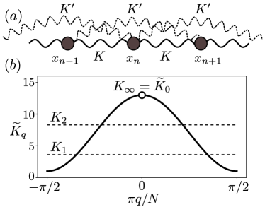
Figure 1: (a) “Toy” model of length scale dependent elasticity consisting of a linear chain with neighbors and next-neighbors springs with stiffnesses $K$ and $K^{\prime}$, respectively (Eq. (1)). (b) Momentum space stiffness of the model (7) for $K=1$ and $K^{\prime}=3$. The one-step $K_{1}$, two-step $K_{2}$ and asymptotic stiffnesses $K_{\infty}=\widetilde{K}_{0}$ (Eqs. (12), (13) and (14)) are shown. In the case shown here ($K^{\prime}>0$) the system is softer at short scales: $K_{1}<K_{2}<\ldots<K_{\infty}$.

II Linear elastic chain with next nearest-neighbor coupling

In order to illustrate the effect of beyond-nearest-neighbor couplings and the procedure of analyzing length-dependent elasticity we first consider a one dimensional “toy” model of a linear elastic chain with next neighbors couplings.

This model (illustrated in Fig. 1(a)) consists of an elastic chain of $N$ masses located at positions $x_{n}$, which are subjected to periodic boundary conditions ($x_{N+1}=x_{0}+(N+1)a$). These boundary conditions are formally necessary for our formalism, however their violation merely constitutes a finite size effect that will vanish for sufficiently large $N$. Interactions between the masses are mediated by two types of springs with stiffnesses $K$ and $K^{\prime}$ and rest lengths $a$ and $2a$, acting respectively between nearest-neighbors and next-nearest neighbors. Accordingly, the energy of the system - in units of $k_{B}T$ - is given by

$$\beta E=\frac{K}{2}\sum_{n=0}^{N-1}(x_{n+1}-x_{n}-a)^{2}+\frac{K^{\prime}}{2}\sum_{n=0}^{N-1}(x_{n+2}-x_{n}-2a)^{2},$$ (1)

with $\beta=1/k_{B}T$. The minimal energy configuration of the system is $x_{n}=x_{0}+na$. We are interested in the stretching fluctuations at different length scales, as captured by the m-step fluctuations

$$\langle(x_{m}-x_{0}-ma)^{2}\rangle=\frac{m}{K_{m}},$$ (2)

for which we define an effective spring constant $K_{m}$. In absence of next-nearest neighbor couplings ($K^{\prime}=0$) one simply finds $K_{m}=K$, as the mean-squared extension of $m$ independent springs is just $m$ times the extension of a single spring, which yields the stated relation by virtue of the equipartition theorem. As we shall show, in the case $K^{\prime}\neq 0$ the spring constant $K_{m}$ depends on $m$, indicating a length dependent elasticity.

For the calculation of $K_{m}$ we define the displacement from the springs rest length as $u_{n}\equiv x_{n+1}-x_{n}-a$, such that (1) becomes

$$\beta E = \frac{K}{2}\sum_{n=0}^{N-1}u_{n}^{2}+\frac{K^{\prime}}{2}\sum_{n=0}^{N-1}(u_{n+1}+u_{n})^{2}.$$ (3)

We introduce the discrete Fourier transform of the displacements

$${\cal U}_{q}=\sum_{n=0}^{N-1}e^{-2\pi iqn/N}\,u_{n},$$ (4)

with $q=-(N-1)/2,-(N-3)/2,\ldots(N-1)/2$ (assuming $N$ odd) referred to as momentum here. Accordingly, the inverse Fourier transform is given by

$${u}_{n}=\frac{1}{N}\sum_{q}e^{2\pi iqn/N}\,{\cal U}_{q},$$ (5)

where the sum runs over the above given values of $q$. Since the $u_{n}$ are real variables we have ${\cal U}_{q}^{*}={\cal U}_{-q}$. In momentum space the energy then becomes

$$\beta E=\frac{1}{2N}\sum_{q}\widetilde{K}_{q}|{\cal U}_{q}|^{2}.$$ (6)

The stiffness of the mode with momentum $q$ obeys

$$\widetilde{K}_{q}\equiv K+4K^{\prime}\cos^{2}\frac{\pi q}{N}.$$ (7)

From here one can easily deduce the stability condition of the system: $\widetilde{K}_{q}>0$ for all $q$ requires $K>0$ and $K^{\prime}>-K/4$. Figure 1(b) shows $\widetilde{K}_{q}$ for $K=1$ and $K^{\prime}=3$.

The equipartition theorem, applied to (6) gives

$$\langle{\cal U}_{q}\,{\cal U}_{q^{\prime}}\rangle=N\widetilde{K}_{q}^{-1}\,\delta_{q,-q^{\prime}},$$ (8)

where $\delta_{n,k}$ is the Kronecker delta. Moreover, collective m-step fluctuations can be expressed as

$$x_{m}-x_{0}-ma=\sum_{n=0}^{m-1}u_{n}=\frac{1}{N}\sum_{q}\frac{\sin\frac{\pi qm}{N}}{\sin\frac{\pi q}{N}}e^{i\pi q(m-1)/N}{\cal U}_{q}.$$ (9)

Combining (2), (8) and (9) we find

$$\frac{m}{K_{m}}=\frac{1}{N^{2}}\sum_{q}\frac{\sin^{2}\frac{\pi qm}{N}}{\sin^{2}\frac{\pi q}{N}}\langle|{\cal U}_{q}|^{2}\rangle=\frac{1}{N}\sum_{q}\frac{\sin^{2}\frac{\pi qm}{N}}{\widetilde{K}_{q}\sin^{2}\frac{\pi q}{N}}.$$ (10)

In the limit $N\to\infty$ one can replace the discrete sum with an integral

$$\frac{1}{K_{m}} = \frac{1}{m\pi}\int_{-\pi/2}^{\pi/2}\frac{\sin^{2}my}{\sin^{2}y}\frac{dy}{K+4K^{\prime}\cos^{2}y},$$ (11)

where we defined $y\equiv\pi q/N$ and used (7). For $m=1$ and $m=2$ a straightforward calculation shows that

$$K_{1}=\sqrt{K(K+4K^{\prime})}$$ (12)

$$K_{2}=\frac{2K^{\prime}\sqrt{K+4K^{\prime}}}{\sqrt{K+4K^{\prime}}-\sqrt{K}}.$$ (13)

In the asymptotic limit of large $m$ the factor $\sin^{2}(my)/\sin^{2}y$ in (11) becomes increasingly peaked around $y=0$. Expanding $1/(K+4K^{\prime}\cos^{2}y)$ to lowest orders in $y$ we obtain in the case $m\gg 1$

$$K_{m}=\widetilde{K}_{0}-\frac{4K^{\prime}\log 2}{m}+{\cal O}\left(\frac{1}{m^{2}}\right),$$ (14)

where we used

$$\int_{-\pi/2}^{\pi/2}\frac{\sin^{2}my}{\sin^{2}y}\,dy = {m\pi},$$ (15)

and

$$\int_{-\pi/2}^{\pi/2}\frac{y^{2}dy}{\sin^{2}y}=\pi\log 4.$$ (16)

Equations (12), (13) and (14) show that the stiffness of the chain depends on the length scale at which fluctuations are observed. In the case $K^{\prime}>0$ one finds $K_{1}<K_{2}<\ldots<K_{\infty}$, eg. the chain becomes increasingly stiffer at longer length scales (Fig. 1(b)). The behavior is the opposite if $K^{\prime}<0$: the chain is softer at longer distances $K_{1}>K_{2}>\ldots>K_{\infty}$. As $m$ increases the contribution of large momenta to $K_{m}$ gradually diminishes, until finally only the zero-momentum component ($q=0$) contributes to the asymptotic stiffness $K_{\infty}=\widetilde{K}_{0}$. In the opposite limit ($m=1$) $K_{1}$ becomes the harmonic mean of the momentum domain stiffnesses $\widetilde{K}_{q}$. Recall that the harmonic mean of $N$ numbers $\omega_{i}$ with $i=1$, $2$ …$N$ is defined as

$$\langle\omega\rangle_{h}=\left(\frac{1}{N}\sum_{i}\frac{1}{\omega_{i}}\right)^{-1}.$$ (17)

We consider now the effect of a local perturbation stretching one of the springs (say $u_{0}$). This can be achieved by imposing a local force $f>0$ on the selected degree of freedom such that the energy becomes

$$\beta E_{f}=\beta E-\beta fu_{0}=\frac{1}{2N}\sum_{q}\widetilde{K}_{q}|{\cal U}_{q}|^{2}-\frac{\beta f}{N}\sum_{q}{\cal U}_{q},$$ (18)

with $\beta E$ the unperturbed energy (6). The force stretches all modes to a non-zero average

$$\langle{\cal U}_{q}\rangle=\frac{\beta f}{\widetilde{K}_{q}}.$$ (19)

The inverse Fourier transform then gives (for details see Appendix 49)

$$\langle u_{m}\rangle = \frac{\beta f}{N}\sum_{q}\frac{e^{2iqm/N}}{\widetilde{K}_{q}}=\frac{\beta f}{\pi}\int_{-\pi/2}^{\pi/2}\frac{e^{2iym}\,dy}{K+4K^{\prime}\cos^{2}y}$$ (20)

$$= \frac{\beta f}{K_{1}}\left[-\text{sgn}(K^{\prime})\right]^{m}\,e^{-m/l_{\text{A}}},$$

with $m>0$, sgn denoting the signum function and

$$\frac{1}{l_{\text{A}}}=-\log\frac{|K_{2}-K_{1}|}{K_{2}}.$$ (21)

Here $K_{1}$ and $K_{2}$ are the one-step and two-step stiffnesses defined in (12), (13). We note that for $m=0$ we get from (20) $K_{1}\langle u_{0}\rangle=\beta f$, showing again that $K_{1}$ is the stretching stiffness between neighboring sites. If $K^{\prime}>0$, the quantity $\langle u_{m}\rangle$ has an oscillatory decay, which can be easily understood from the coupling term $K^{\prime}u_{n}u_{n+1}$, that contributes negatively if neighboring $u_{n}$ have opposite signs. The same reasoning explains the monotonic decay if $K^{\prime}<0$. Note that in absence of length scale dependence, which means that $K_{m}$ does not depend on $m$, one has $l_{\text{A}}=0$. Hence, in that case, a local perturbation does not affect flanking springs.

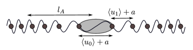
Figure 2: Schematic illustration of the effect of a local perturbation at site $n=0$ resulting in an exponentially decaying stretching profile $\langle u_{m}\rangle$, see Eq. (20). This depiction represents the case $K^{\prime}<0$, where the stretching decays monotonically (for the sake of clarity we do not show next-neighbors springs).

To conclude the analysis of the model we remark that while our discussion here was limited to interactions ranging to next-nearest neighbors, i.e. involving just two spring constants ($K$and $K^{\prime}$), the same formalism is directly applicable to systems involving further ranging interactions. In that case (10) and (20) remain valid, but $\widetilde{K}_{q}$ will assume a more complicated form.

III DNA elasticity in momentum space

In our coarse-grained description of DNA any configuration of a molecule consisting of $N+1$ base pairs is fully described by a set of $N+1$ orthonormal triads $\widehat{\cal T}_{n}=(\widehat{\bf f}_{n}\widehat{\bf v}_{n}\widehat{\bf u}_{n})$, where $\widehat{\bf f}_{n},\widehat{\bf v}_{n}$ and $\widehat{\bf u}_{n}$ are unit vectors capturing the local geometry of the base pair. We define $\widehat{\bf u}_{n}$ to be the local tangent and $\widehat{\bf v}_{n}$ to connect the two oppositely running backbones such that the remaining vector $\widehat{\bf f}_{n}=\widehat{\bf v}_{n}\times\widehat{\bf u}_{n}$ points towards the major groove (in the literature this frame is indicated also as $(\widehat{\bf e}_{1}\widehat{\bf e}_{2}\widehat{\bf e}_{3})$ Marko and Siggia (1994); Skoruppa et al. (2017), here we use a different notation to avoid double indexing $\widehat{\bf e}_{1,n}$). The spacial configuration of the molecule is given by the set of points connected by the vectors $a\widehat{\bf u}_{n}$, where $a$ is the distance between consecutive base pairs. We assume this distance to be the constant value $a=0.34$ nm. For simplicity this description ignores stretching deformations. However, such could easily be included by replacing the connection vector $a\widehat{\bf u}_{n}$ by a variable $3$-component vector.

Up to a global rotation a particular chain configuration is fully captured by the set of rotations that map each triad onto its consecutive triad, as illustrated in Fig. 3. It is convenient to parametrize these rotations by the corresponding Euler vectors $\mathbf{\Theta}$, i.e. the vectors parallel to the rotation axis with magnitude $\Theta=|\mathbf{\Theta}|$ equal to the rotation angle. In order to link the vector components to the local geometry we express it in the basis of the local material frame

$$\mathbf{\Theta}_{n}=a\tau_{n}\widehat{\bf f}_{n}+a\rho_{n}\widehat{\bf v}_{n}+a(\Omega_{n}+\omega_{0})\widehat{\bf u}_{n}.$$ (22)

The components $\tau$ and $\rho$ denote the two bending modes commonly referred to as tilt and roll Lavery et al. (2009b), quantifying local bending over the axes $\widehat{\bf f}_{n}$ and $\widehat{\bf v}_{n}$ respectively. The total twist $\Omega_{n}+\omega_{0}$ (rotation around $\widehat{\bf u}_{n}$) has two components: $\Omega_{n}$ is the excess twist and $\omega_{0}=1.75\,\text{nm}^{-1}$ the intrinsic twist of the double helix, corresponding to one turn of the helix every $10.5$ base pairs. The deformation densities $\tau_{n}$, $\rho_{n}$ and $\Omega_{n}$ of (22) have the dimension of inverse lengths and are expressed in nm^-1, while $a\tau_{n}$, $a\rho_{n}$ and $a\Omega_{n}$ are dimensionless and express rotation angles in radians.

The configuration $\tau_{n}=\rho_{n}=\Omega_{n}=0$ (all $n$) corresponds to a straight twisted rod with intrinsic twist $\omega_{0}$, which is assumed to be the ground state of the system. Any deformation away from this state will be associated with a certain free energy. Expanding this free energy to lowest non-vanishing order around the ground state then corresponds to a regime of linear elasticity. In this work we limit our discussion to this regime. It is customary to describe DNA elasticity using on-site models, e.g. without interactions between neighboring sites. For instance, the Marko-Siggia model Marko and Siggia (1994) is defined as

$$\beta E=\frac{a}{2}\sum_{n}\left(A^{t}\tau_{n}^{2}+A^{r}\rho_{n}^{2}+C\Omega_{n}^{2}+2G\rho_{n}\Omega_{n}\right),$$ (23)

where $A^{t}$, $A^{r}$, $C$ and $G$ are stiffness parameters (we neglect in this description sequence dependent effects and use constant stiffnesses). Besides the individual stiffnesses of tilt ($A^{t}$), roll ($A^{r}$) and twist ($C$), the model (23) is characterized by a non-vanishing twist-roll coupling ($G$), as expected from the symmetry of the molecule Marko and Siggia (1994). The effects of this coupling in the conformations of a DNA molecule were discussed recently in Skoruppa et al. (2018); Caraglio et al. (2019); Nomidis et al. (2019a).

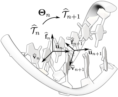
Figure 3: Mapping of a DNA configuration into a rigid basepair representation Lankaš et al. (2009) that consists of a series of triads each attached to a single basepair, capturing the local geometry of the molecule. These triads are constructed from a set of 3 mutually orthogonal unit vectors $\widehat{\cal T}_{n}=(\widehat{\bf f}_{n}\widehat{\bf v}_{n}\widehat{\bf u}_{n})$, where $\widehat{\bf u}_{n}$ is the local tangent, $\widehat{\bf v}_{n}$ connects the two backbones and $\widehat{\bf f}_{n}$ points towards the major groove. Deformation of the chain are parametrized by the rotation vectors $\mathbf{\Theta}_{n}$ rotating the triads $\widehat{\cal T}_{n}$ into their sequentially adjacent triads $\widehat{\cal T}_{n+1}$.

We generalize the elastic model to allow for interactions between further neighbors employing a matrix representation

$$\beta E=\frac{a}{2}\sum_{n}\sum_{m}\mathbf{\Delta}_{n}^{\intercal}M_{m}\mathbf{\Delta}_{n+m},$$ (24)

with $\mathbf{\Delta}_{n}^{\intercal}=(\tau_{n},\rho_{n},\Omega_{n})$ and where the $M_{m}$ are $3\times 3$ matrices describing the couplings between sites separated by $m$ steps. Stability of the model requires the on-site matrices $M_{0}$ to be positive definite. For homogeneous directionally invariant chains the general form of the matrices $M_{m}$ can be deduced from symmetry considerations. Reversal of the curvilinear coordinate system, i.e. a definition of the $\mathbf{\Theta}_{n}$ in backwards-sense rather than forwards-sense results in the same stiffness matrices, however for a given configuration this sense-reversal transformation leads to the transformation $\mathbf{\Delta}_{n}^{\intercal}=(\tau_{n},\rho_{n},\Omega_{n})\to(-\tau_{n},\rho_{n},\Omega_{n})=\mathbf{\bar{\Delta}}_{n}^{\intercal}$ Marko and Siggia (1994). Since this coordinate transformation cannot change the energy we see that for every $m$

$$\mathbf{\Delta}_{n}^{\intercal}M_{m}\mathbf{\Delta}_{n+m}=\mathbf{\bar{\Delta}}_{n+m}^{\intercal}M_{m}\mathbf{\bar{\Delta}}_{n}.$$ (25)

This implies that all off-diagonal terms in $M_{m}$ involving $\tau$, have to be anti-symmetric, while the remaining coupling (between $\rho$ and $\Omega$) is required to be symmetric. Hence, for homogeneous chains, the most general form of the matrices $M_{m}$ is

$$M_{m}=\begin{pmatrix}\phantom{-}A_{m}^{t}&A_{m}^{tr}&B_{m}\\ -A_{m}^{tr}&A_{m}^{r}&G_{m}\\ -B_{m}&G_{m}&C_{m}\\ \end{pmatrix}.$$ (26)

For example, the coupling $A_{m}^{tr}$ gives rise to terms of the form

$$\frac{1}{2}\sum_{n}{A}^{tr}_{m}\left({\tau}_{n}{\rho}_{n+m}-{\rho}_{n}{\tau}_{n+m}\right).$$ (27)

This symmetry consideration implies that for homogeneous on-site models, i.e. $M_{m}=0$ for $m\geq 1$, the most general form of the free energy density (in the regime of linear elasticity) is given by the afore mentioned Marko-Siggia model (23). In matrix representation this corresponds to a $M_{0}$ of the form (26) with $A^{tr}_{0}=B_{0}=0$.

We can rewrite the model (24) in momentum space as

$$\beta E=\frac{a}{2N}\sum_{q}\widetilde{\mathbf{\Delta}}_{q}^{\dagger}\widetilde{M}_{q}\widetilde{\mathbf{\Delta}}_{q},$$ (28)

where $\widetilde{\mathbf{\Delta}}_{q}$ and $\widetilde{M}_{q}$ are the Fourier transform of $\mathbf{\Delta}_{n}$ and $M_{m}$, respectively, and ^$\dagger$ indicates the conjugate transpose. Stability of the model requires each of the Hermitian matrices $\widetilde{M}_{q}$ to be be positive definite, i.e. that all eigenvalues are positive. As indicated in (26) the matrices $M_{m}$ may contain symmetric and anti-symmetric components. Fourier transformation in $m$ of the matrices (26) gives

$$\widetilde{M}_{q}=\begin{pmatrix}\phantom{-}\widetilde{A}^{t}_{q}&i\widetilde{A}^{tr}_{q}&i\widetilde{B}_{q}\\ -i\widetilde{A}^{tr}_{q}&\widetilde{A}^{r}_{q}&\widetilde{G}_{q}\\ -i\widetilde{B}_{q}&\widetilde{G}_{q}&\widetilde{C}_{q}\\ \end{pmatrix},$$ (29)

where all entries $\widetilde{A}^{t}_{q}$, $\widetilde{A}^{r}_{q}$, $\widetilde{A}^{tr}_{q}$, $\widetilde{B}_{q}$, $\widetilde{C}_{q}$, and $\widetilde{G}_{q}$ are real variables. The off-diagonal terms $\widetilde{A}^{tr}_{q}$, $\widetilde{B}_{q}$ are odd functions of $q$ (e.g. $\widetilde{A}^{tr}_{-q}=-\widetilde{A}^{tr}_{q}$), while all other terms are even functions of $q$.

The advantage of the momentum space representation is that modes with different $q$ are independent (except for the coupling between $q$ and $-q$). Strictly speaking, this is valid only if periodic boundary conditions are imposed such that full translational invariance is achieved. In absence of that, some boundary terms will appear, which, however, will be negligible for sufficiently large $N$.

Given an ensemble of deformation vectors $\mathbf{\Delta}_{n}$ the stiffness matrices can be obtained from the relation Olson et al. (1998)

$$\langle\widetilde{\mathbf{\Delta}}_{q}\widetilde{\mathbf{\Delta}}_{q}^{\dagger}\rangle = \frac{N}{a}\widetilde{M}_{q}^{-1},$$ (30)

where the $3\times 3$ covariance matrix $\langle\widetilde{\mathbf{\Delta}}_{q}\widetilde{\mathbf{\Delta}}_{q}^{\dagger}\rangle$ is constructed from the ensemble averages of the products of the three components of the vector $\widetilde{\mathbf{\Delta}}_{q}^{\intercal}=(\widetilde{\tau}_{q},\widetilde{\rho}_{q},\widetilde{\Omega}_{q})$. In the remainder of this section we discuss the consequences of this model extension on various DNA properties: length dependence of persistence lengths and decays of local perturbations.

III.1 Twist persistence length

The twist-correlation function is defined as

$${\cal C}_{\mathrm{T}}(m)=\left\langle\cos\left(a\sum_{n=0}^{m-1}\Omega_{n}\right)\right\rangle=\text{Re}\left\langle e^{\,\,\displaystyle ia\sum_{n=0}^{m-1}\Omega_{n}}\right\rangle,$$ (31)

where Re denotes the real part. We are interested in the twist persistence length, which is the characteristic decay-length of twist-correlations

$$\frac{1}{l_{\text{T}}}=-\frac{1}{ma}\,\log{\cal C}_{\mathrm{T}}(m).$$ (32)

At this point, we present only a sketch of the calculation, as it is totally analogous to that of the elastic chain example discussed in detail in Sec. II. In like manner, we rewrite the sum in (31) in momentum space using the expression (9). The variables $\widetilde{\Omega}_{q}$ for different momenta are independent hence the total average (31) factorizes in terms of the form $\langle\exp(i\alpha_{q}\widetilde{\Omega}_{q}+i\alpha_{-q}\widetilde{\Omega}_{-q})\rangle$ (it is convenient to group terms $q$ and $-q$ together). Using the property of Gaussian variables

$$\left\langle e^{\displaystyle\pm i\alpha X}\right\rangle=e^{\displaystyle-\frac{\alpha^{2}}{2}\langle X^{2}\rangle},$$ (33)

we obtain in the limit $N\to\infty$

$$\frac{1}{l_{\text{T}}} = \frac{a}{2\pi m}\int_{-\pi/2}^{\pi/2}\frac{\sin^{2}my}{\sin^{2}y}\frac{\langle|\widetilde{\Omega}_{q}|^{2}\rangle}{N}\,dy,$$ (34)

which is analogous to (11) and where we again used $y\equiv\pi q/N$. Just as in the example of Sec. II the integral is dominated by smaller and smaller $y$ contributions as $m$ increases. The asymptotic twist persistence length ($m\to\infty$) is finally entirely governed by the zero-momentum component

$$\frac{1}{l_{\text{T}}}=\frac{a}{2N}\langle\widetilde{\Omega}_{0}^{2}\rangle.$$ (35)

III.2 Bending persistence length

From the tangent-tangent correlation function

$${\cal C}_{\mathrm{B}}(m)=\langle\widehat{\bf u}_{0}\cdot\widehat{\bf u}_{m}\rangle$$ (36)

one obtains the bending persistence length

$$\frac{1}{l_{\text{B}}}=-\frac{1}{ma}\,\log{\cal C}_{\mathrm{B}}(m).$$ (37)

The twist-correlation function could be expressed exactly in terms of the deformation vectors $\mathbf{\Delta}_{n}$. However, establishing such a connection for ${\cal C}_{\mathrm{B}}$ requires some approximations. Under the assumption that the rotations connecting neighboring triads are dominated by the intrinsic twist component $\omega_{0}$, we derived the following expression for the bending persistence length (for details see Appendix B)

$$\frac{1}{l_{\text{B}}}=\frac{a}{\pi m}\int_{-\pi/2}^{\pi/2}\frac{\sin^{2}my}{\sin^{2}y}\,\frac{\Psi_{q+\Delta q}+\Psi_{q-\Delta q}}{N}\,dy,$$ (38)

where we defined $\Delta q=Na\omega_{0}/(2\pi)$ and

$$\Psi_{q}\equiv\frac{1-\cos(a\omega_{0})}{2(a\omega_{0})^{2}}\left\langle\left|\widetilde{\tau}_{q}\right|^{2}+\left|\widetilde{\rho}_{q}\right|^{2}\right\rangle.$$ (39)

This relation resembles Eq. (34) with the difference that here the $y(q)$ contributions of the momentum space bending deformations (tilt and roll) are replaced by the mean of the shifted momenta $q\pm\Delta q$. This stems from the fact that in order to appropriately connect local bending deformations to the total deformation of a given multi-step segment (say from $\widehat{\mathbf{u}}_{0}$ to $\widehat{\mathbf{u}}_{m}$) one needs to rotate the local reference frames to unwind the intrinsic helical twist. $\Delta q$ is indeed the momentum shift associated with the DNA intrinsic twist. As we integrate in the rescaled variable $y=\pi q/N$, the momentum shift corresponds to $\Delta y=a\omega_{0}/2\approx\pi/10.5$, e.g. approximately one tenth of the $y$ domain ($10.5$ is the number of base pairs for a full turn of the double helix). In the limit $m\to\infty$ the $q=y=0$ term is selected from the integral, and the asymptotic persistence length becomes (using (15))

$$\frac{1}{l_{\text{B}}}=\frac{1-\cos(a\omega_{0})}{a\omega_{0}^{2}N}\left\langle\left|\widetilde{\tau}_{\Delta q}\right|^{2}+\left|\widetilde{\rho}_{\Delta q}\right|^{2}\right\rangle.$$ (40)

III.3 Local perturbations

Repeating the procedure applied to the linear chain model of Section II we add a local perturbation at a given site of the DNA. This perturbation is introduced by means of generalized “forces” acting on the rotational degrees of freedom associated with that site - again we choose the site $n=0$, but translational invariance implies that the results are equally valid for any given site - so that the energy becomes

$$\beta E_{\mathbf{f}} = \beta E-\beta\mathbf{f}^{\intercal}\mathbf{\Delta}_{0}$$ (41)

$$= \frac{a}{2N}\sum_{q}\left(\widetilde{\mathbf{\Delta}}_{q}^{\intercal}-\frac{\beta}{a}\mathbf{f}^{\intercal}\widetilde{M}_{q}^{-1}\right)\widetilde{M}_{q}\left(\widetilde{\mathbf{\Delta}}_{q}-\widetilde{M}_{q}^{-1}\frac{\beta}{a}\mathbf{f}\right)$$

$$- \frac{\beta^{2}}{2Na}\mathbf{f}^{\intercal}\widetilde{M}_{q}^{-1}\mathbf{f}$$

where $\beta E$ is the unperturbed energy (28) and $\mathbf{\Delta}_{0}^{\intercal}=(\tau_{0},\rho_{0},\Omega_{0})$. The vector $\mathbf{f}^{\intercal}=(f_{\tau},f_{\rho},f_{\Omega})$ contains three components coupling to tilt, roll and twist, respectively. These generalized forces shift the average $\widetilde{\mathbf{\Delta}}_{q}$ to the non-zero value

$$\langle\widetilde{\mathbf{\Delta}}_{q}^{\intercal}\rangle=\frac{\beta}{a}\mathbf{f}^{\intercal}\widetilde{M}_{q}^{-1},$$ (42)

which is the equivalent of (19). In the DNA case the calculation involves the inversion of the $3\times 3$ matrix $\widetilde{M}_{q}$

$$\widetilde{M}_{q}^{-1}=\frac{\text{Adj}\left[\widetilde{M}_{q}\right]}{\text{det}\,\widetilde{M}_{q}},$$ (43)

where $\text{Adj}[.]$ denotes the adjoint matrix. Combining (42) and (43) and performing the inverse Fourier transform we obtain

$$\langle\mathbf{\Delta}_{m}^{\intercal}\rangle = \frac{\beta}{\pi}\int_{-\pi/2}^{\pi/2}\frac{\mathbf{f}^{\intercal}\,\text{Adj}\left[\widetilde{M}_{q}\right]}{\text{det}\,\widetilde{M}_{q}}\,e^{2iym}\,dy,$$ (44)

which is analogous to Eq. (20), derived for the toy model. As in that case, Eq. (44) gives rise to an exponential decay for large $m$: $\langle\mathbf{\Delta}_{m}\rangle\sim\exp(-ma/l_{\text{A}})$. The characteristic decay length $l_{\text{A}}$ is given by the poles closest to the real axis of the integrand (see Appendix 49). We note that stability of the energy (28) requires $\text{det}\,\widetilde{M}_{q}>0$ in the real $q$ domain. Hence poles have necessarily an imaginary component responsible for the exponential decay. In practice this integral can be evaluated numerically from empirically obtained $\widetilde{M}_{q}$.

IV DNA elasticity in coarse-grained and all-atom models

We discuss and compare here the elasticity of the coarse grained DNA model oxDNA Ouldridge et al. (2010), and of an all atom model. The main focus is the calculation of $\widetilde{M}_{q}$ from which various quantities are obtained, following the framework discussed in the previous Section.

IV.1 oxDNA

The oxDNA model treats nucleotides as single rigid objects, that mutually interact via multiple sites representing the most significant inter-base interactions: backbone-connectivity, base-pairing and base-stacking. These interactions are parametrized so as to reproduce thermodynamical, structural and mechanical properties of DNA Ouldridge et al. (2010). oxDNA has been used to study a broad range of processes such as DNA-melting, -hybridization, -supercoiling, -looping, DNA strand-displacement mechanisms , DNA gels, nanotubes and origami Srinivas et al. (2013); Schmitt et al. (2013); Matek et al. (2015); Romano and Sciortino (2015); Engel et al. (2018); Desai et al. (2020); Chhabra et al. (2020). Here we focus exclusively on oxDNA2 Snodin et al. (2015), a version of the model with asymmetric major and minor grooves. We used the procedure outlined in Skoruppa et al. (2017) to map the oxDNA coordinates to orthonormal triads $(\widehat{\mathbf{f}}_{n}\widehat{\mathbf{v}}_{n}\widehat{\mathbf{u}}_{n})$ (Fig. 3). This mapping is not unique and a few alternative definitions have been discussed in Skoruppa et al. (2017). Differences in triads are carried over the to rotational modes $\mathbf{\Delta}_{n}$, which leads to slightly different elastic behavior. However, we observe the Fourier spectra of the couplings to exhibit the same general features. In particular, alternative triads give the same behavior at small $q$ (same asymptotic elasticity) and follow the same trend from small to large $q$ behavior. We will present here the results from triad2, as defined in Skoruppa et al. (2017).

Using molecular dynamics trajectories of oxDNA2 (details about simulations can be found in Skoruppa et al. (2017)) we computed the Fourier spectra of the rotational deformations $\widetilde{\mathbf{\Delta}}_{q}^{\intercal}=(\widetilde{\tau}_{q},\widetilde{\rho}_{q},\widetilde{\Omega}_{q})$. The stiffness matrices $\widetilde{M}_{q}$ were then obtained by utilizing Eq. (30). The matrix entries vs. rescaled momentum $y\equiv\pi q/N$ are plotted in Fig. 4(a). These matrices indeed follow the structure (29) as predicted by the symmetry consideration. The anti-symmetric components turn out to be very small, with $\widetilde{B}_{q}$ virtually zero. The only significant off-diagonal term in oxDNA2 is the twist-roll coupling $\widetilde{G}_{q}$ Skoruppa et al. (2017). We note that $\widetilde{A}^{r}_{q}$, the roll stiffness is very weakly dependent on $q$ as compared to the other entries. This weak dependence indicates that the roll-roll interaction is dominated by the on-site term $\rho_{n}^{2}$. The strong dependence on $q$ for tilt-tilt and twist-twist terms implies significant contributions from off-site interactions $\tau_{n}\tau_{n+m}$ and $\Omega_{n}\Omega_{n+m}$, with $m>0$.

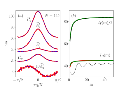
Figure 4: (a) Red dots: Simulation data reporting the entries of the stiffness matrix in momentum space $\widetilde{M}_{q}$ for oxDNA2 as obtained from Eq. (30) for a sequence of length $150$. In the analysis two nucleotides at the two ends were eliminated, which gives $146$ triads and thus $N=145$ deformation vectors $\mathbf{\Delta}_{m}$. The units are in nm. The entry $\widetilde{A}^{tr}_{q}$ has been multiplied by a factor $10$ to facilitate its visibility. The stiffness matrix has the structure given in (29). All its entries are symmetric in $q$, except for the tilt-roll term $\widetilde{A}^{tr}_{q}$ which is anti-symmetric. Blue dashed lines: Fits of the data to Eqs. (45) and (46), with fitting parameters given in Table 1. (b) Plots of $l_{\text{B}}$ and $l_{\text{T}}/2$ vs. $m$ the relative distance in numbers of basepair-steps between the considered segments. Green lines are obtained from the stiffness matrix data using Eqs. (34) and (38). The red line is the approximation (70). In this case the difference between the two approximations for $l_{\text{B}}$ is very small. Black dashed lines are obtained by direct calculations of correlation functions from simulations. The oscillatory behavior of the bending persistence length stems from a light helicity of the traced contour.

Table 1: Summary of the stiffnesses in oxDNA2 (data in nm). $X_{m}$ are the fitting coefficients used in Eqs. (45) and (46). The two rightmost columns give the stiffnesses at $q=0$ and $q=\Delta q$, as representatives of the long length scale behavior (see Eqs. (35) and (40)). The last two lines give the persistence lengths as obtained from Eqs. (34) and (38). We give the local ($m=1$) value and the asymptotic one ($m\to\infty$). All parameters are given in nm.

	$X_{0}$	$X_{1}$	$X_{2}$	$X_{3}$	$q=0$	$q=\Delta q$
$\widetilde{A}^{t}_{q}$	54	17	4.0	1.1	76	69
$\widetilde{A}^{r}_{q}$	38	2	0.8	0.2	41	40
$\widetilde{C}_{q}$	78	22	6.5	1.3	108	98
$\widetilde{G}_{q}$	23	6.0	1.9	0.4	31	28
$\widetilde{A}^{tr}_{q}$		-0.9			0	-0.5
$l_{\text{B}}$		40 ($m=1$)		45 ($m\to\infty$)
$l_{\text{T}}/2$		63 ($m=1$)		84 ($m\to\infty$)

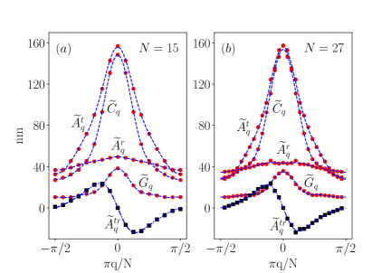
Figure 5: Red dots and solid squares: Elements of the stiffness matrix $\widetilde{M}_{q}$ as obtained from all-atom data for sequences of length (a) $N=20$ (average of $9$ seq.) and (b) $N=32$ (average of $3$ seq.). Dashed lines: fits of the forms (45) and (46).

To quantify these effects the inverse Fourier transform of the data in Fig. 4(a) was computed so as to obtain the couplings in real space . The Fourier series of the elements of the stiffness matrix which are even or odd in $q$ are given by

$$\widetilde{X}_{q}^{\text{even}} = \sum_{m}X_{m}\cos\frac{2m\pi q}{N},$$ (45)

$$\widetilde{X}_{q}^{\text{odd}} = \sum_{m}X_{m}\sin\frac{2m\pi q}{N},$$ (46)

where $X_{m}$ are the real-space stiffness associated to couplings between sites $n$ and $n+m$ .

For the even terms we truncated the series to the first four components, while in view of the uncertainties of the small odd term $\widetilde{A}^{tr}_{q}$ we used a single term. The best fits to the data are shown as dashed blue lines in Fig. 4(a). Table 1 gives the values of the corresponding coefficients $X_{m}$ resulting from the fits. The coefficients decrease rapidly with $m$, but there are significant off-site components for $\widetilde{C}_{q}$ and $\widetilde{A}^{r}_{q}$, reflecting the strong $q$-dependence observed in Fig. 4(a). Twist and bend fluctuations are linked to the elements of the stiffness matrix via the covariance matrix (30). Neglecting the small contribution of $\widetilde{A}^{tr}_{q}$, and inverting $\widetilde{M}_{q}$ we get

$$\frac{a\langle|\widetilde{\Omega}_{q}|^{2}\rangle}{N}=\frac{1}{\widetilde{C}_{q}-\widetilde{G}_{q}^{2}/\widetilde{A}^{r}_{q}},$$ (47)

and

$$\frac{a\langle|\widetilde{\tau}_{q}|^{2}+|\widetilde{\rho}_{q}|^{2}\rangle}{N}=\frac{1}{\widetilde{A}^{t}_{q}}+\frac{1}{\widetilde{A}^{r}_{q}-\widetilde{G}_{q}^{2}/\widetilde{C}_{q}},$$ (48)

Inserting (47) in (34) we can estimate the twist persistence length $l_{T}(m)$ from the stiffness data using the truncated Fourier series as numerical estimates for $\widetilde{A}^{r}_{q}$, $\widetilde{G}_{q}$ and $\widetilde{C}_{q}$. In a similar way inserting (48) into Eq. (38) allows us to calculate the bending persistence length. The results of these calculations are shown in Fig. 4(b) as solid green lines. The red solid line is the approximation (70) . Dashed black lines show the direct calculations of the bending persistence length as deduced from the decay length of the respective correlation functions ((31) and (36)). While there is excellent overlap between dashed and solid lines for $l_{\text{T}}$, some deviations of a few $nm$ are visible in $l_{\text{B}}$. The overlap in $l_{\text{T}}$ was expected as (34) is exact, while both expressions (70) and (38) (red and green lines in Fig. 4(b)) involve approximations. Note also, that $l_{\text{B}}$ as deduced from the correlation function exhibits damped oscillatory behavior stemming from a light helicity of the used set of triads.

The last two lines of Table 1 give the local ($m=1$) and asymptotic ($m\to\infty$) values of the persistence lengths as obtained from (34) and (38). Both bending and torsional persistence lengths are smaller at short distances as compared to their asymptotic values, however the effect is modest for $l_{\text{B}}$, while much stronger length-dependent variability is observed in $l_{\text{T}}$. This can be understood from the elements of the stiffness matrix. Torsional persistence is primarily determined by $\widetilde{C}_{q}$ (Eq. (47)) which has a large $q$ dependence, causing strong length scale effects in $l_{\text{T}}$. On the other side the bending stiffness is determined by the harmonic mean of tilt and rescaled roll stiffnesses (48), which is dominated by the softer roll component. The weak dependence of $\widetilde{A}^{r}_{q}$ on q in Fig. 4(a), indicating small off-site roll-roll couplings, is the cause of the modest length scale dependence of $l_{\text{B}}$.

IV.2 All-atom

All-atom simulations of double stranded DNA of two different lengths were performed. Details of setup, force fields, methodology and sequences used can be found in Appendix C. Tilt, roll and twist variables were obtained from simulation data using an own implementation of the algorithm underlying Curves+ Lavery et al. (2009b). Subtracting the averages we obtained the excess values $\mathbf{\Delta}_{n}^{\intercal}=(\tau_{n},\rho_{n},\Omega_{n})$. Local elasticity in all-atom models of DNA is dependent on the type of base pairs, as opposed to the homogeneous oxDNA model. Using the relation (30) we derived an effective stiffness matrix $\widetilde{M}_{q}$. The procedure builds up an equivalent homogeneous model which shares the same covariance matrix as the original data set by matching the second moments of the fluctuations in Fourier space. For a system breaking translational invariance, in general, the correlator $\langle\widetilde{\mathbf{\Delta}}_{q}\widetilde{\mathbf{\Delta}}_{q^{\prime}}^{\dagger}\rangle$ is non-zero also for $q\neq q^{\prime}$. In constructing the average stiffness matrix we ignore these off-diagonal terms, which are expected to have weaker effect as the system size grows, where effective translation invariance is recovered.

Figure 5 shows the elements of $\widetilde{M}_{q}$ in function of $y=\pi q/N$ as obtained from this procedure (red dots and black squares). The lengths simulated correspond to (a) $20$-mers and (b) $32$-mers, averaged over $10$ and $3$ different sequences, respectively. Two nucleotides at each end were removed from the analysis to mitigate end effects. Hence Fig. 5 shows the Fourier transforms on (a) $N=15$ and (b) $N=27$ data points. Despite the difference in length, the two sets exhibit quantitatively very similar stiffnesses. The data share several common features with the oxDNA simulations of Fig. 4: the tilt $\widetilde{A}^{t}_{q}$ and twist $\widetilde{C}_{q}$ stiffnesses are strongly $q$-dependent, indicating considerable contributions from off-site interactions. Just as for oxDNA the roll stiffness $\widetilde{A}^{r}_{q}$ depends very weakly on $q$ and again the only symmetric off-diagonal term of the stiffness matrix is the twist-roll coupling $\widetilde{G}_{q}$. Contrasting oxDNA in all-atom data the tilt stiffness is larger than the twist stiffness $\widetilde{A}^{t}_{q}>\widetilde{C}_{q}$ and their values are quantitatively much larger. In addition the $q$-odd tilt-roll coupling $\widetilde{A}^{tr}_{q}$ is much more prominent than in oxDNA.

Table 2: All atom data for $20$-mers ($N=15$) and $32$-mers ($N=27$) averaged over $10$ and $3$ different oligomers respectively. All parameters are given in nm.

N=15	$X_{0}$	$X_{1}$	$X_{2}$	$X_{3}$	$X_{4}$	$q=0$	$q=\Delta q$
$\widetilde{A}^{t}_{q}$	82	56	11	5.8	1.3	156	130
$\widetilde{A}^{r}_{q}$	43	5.9	-0.4	0.6	0.3	50	48
$\widetilde{C}_{q}$	65	52	21	8.5	1.9	148	112
$\widetilde{G}_{q}$	17	11	5.4	2.9	1.4	38	27
$\widetilde{A}^{tr}_{q}$		-19	-8.4	0.3	-0.6	0	-21
N=27	$X_{0}$	$X_{1}$	$X_{2}$	$X_{3}$	$X_{4}$	$q=0$	$q=\Delta q$
$\widetilde{A}^{t}_{q}$	75	57	14	6.7	2.6	156	125
$\widetilde{A}^{r}_{q}$	40	4.7	-0.4	-0.2	-0.5	43	44
$\widetilde{C}_{q}$	67	53	23	9.3	1.4	154	116
$\widetilde{G}_{q}$	17	9.3	5.0	2.9	1.0	35	25
$\widetilde{A}^{tr}_{q}$		-16	-8.9	0.4	-1.2	0	-21
$l_{\text{B}}$		42 ($m=1$)		61 ($m\to\infty$)
$l_{\text{T}}/2$		43 ($m=1$)		125 ($m\to\infty$)

Table 2 shows the results of the fits of the elements of $\widetilde{M}_{q}$ to Eqs. (45) and (46). The coefficients $X_{m}$ decrease significantly with $m$, but more gradually as compared to oxDNA, indicating more pronounced off-site interactions. Overall, there is a only a small difference between the two data-sets, which is indicative for weak finite size effects. Using the coefficients $X_{m}$ of the $N=27$ data set as representatives for the couplings of a long DNA sequence we invoked (34) and (38) to estimate the twist and bending persistence lengths. Results are shown in Fig. 6(a). As in oxDNA $l_{\text{T}}$ has a strong length scale dependence, while for $l_{\text{B}}$ this dependence in much more modest. The variability of $l_{\text{T}}$ across different length scales is much larger in the all-atom data than in oxDNA. This is due to the much stronger $q$-dependence of the stiffnesses of the former as can be seen when comparing Fig. 5 to Fig. 4. Interestingly, $l_{\text{T}}/2$ approaches an asymptotic value close to $130$ nm, which is not far from the torsional stiffnesses ($120$ nm) measured in magnetic tweezers Lipfert et al. (2014). This technique probes the torsional elasticity by tracing the twist fluctuations of the ends of stretched DNA molecules of several kilobases length. The recent atomistic simulation study by Velasco-Berreleza et al. Velasco-Berrelleza et al. (2020) found a similarly strong length-dependence of the torsional fluctuations, although their asymptotic estimate indicates $l_{\text{T}}/2\approx 90$ nm. We note here that $l_{\text{T}}$ at all length scales is not only determined by the twist stiffness $\widetilde{C}_{q}$, but also by other stiffnesses. In oxDNA twist fluctuations are also influenced by $\widetilde{G}_{q}$ and $\widetilde{A}^{tr}_{q}$, see Eq. (47). The relation is even more elaborate if one includes the tilt-roll coupling $\widetilde{A}^{tr}_{q}$, which is non-negligible in all atom data.

Figure 6(b) shows our calculation of the response of a DNA molecule to a generalized force imposed on a certain basepair-step, as given by the integral (44). The generalized force $(f_{\tau},f_{\rho},f_{\Omega})$ was tuned in order to shift the average deformations ($\langle\tau_{0}\rangle$, $\langle\rho_{0}\rangle$ and $\langle\Omega_{0}\rangle$) from zero to some finite angles ($20^{o}$, $25^{o}$ and $-20^{o}$ for tilt, roll and twist respectively). Due to the presence of non-local couplings, neighboring steps are expected to also be effected by this imposed force. The calculation shows that the resulting shift in the average values decay very rapidly to zero, which is the unperturbed value, with angles being negligibly small already at $m=2$. Although off-site couplings are capable of carrying the effect of a local perturbation to distant flanking sites, the characteristic decay length $l_{\text{A}}$ is quite small. Why are the twist and, to a more limited extent, the bending elasticity varying so much with the length scale (Fig. 6(a)), while local pertubations (Fig. 6(b)) decay so rapidly? To understand this issue it is useful to go back to the toy model of Section II. At different length scales the elasticity is governed by different stiffnesses ranging from $K_{1}$ to $K_{\infty}$, where the asymptotic value is approached as $1/m$ for large $m$ (see Eq. (14)). A local perturbation, on the contrary, decays exponentially with a length linked to the relative difference between the two local elastic constants $K_{1}$ and $K_{2}$, see Eq. (21).

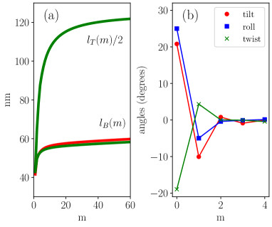
Figure 6: (a) Estimated length scale dependence of the persistence lengths as obtained from the analysis of the all-atom data in Table 2. Assuming that these data are representatives for the behavior of very long sequences, we used Eqs. (38) and (34) to calculate $l_{\text{B}}$ and $l_{\text{T}}$ (green lines). The red line is the approximation (70) for $l_{\text{B}}$. (b) Calculation of the the propagation of pertubations induced by generalized forces acting on the site $m=0$. This data is calculated with Eq. (44) using the data in Table 2. Results are given in degrees (the quantities plotted are $180\,a\tau/\pi$, $180\,a\rho/\pi$ and $180\,a\Omega/\pi$).

V Discussion

In this paper we investigated the effects of interactions in DNA models that extend beyond nearest-neighbors (off-site couplings). Our analysis is based on the calculation of the stiffness matrix in momentum space $\widetilde{M}_{q}$ for oxDNA and all-atom models. Both systems show very similar behavior, which is presumably a consequence of the geometrical structure of the double helix. The set of matrices $\widetilde{M}_{q}$ encodes both the asymptotic long length scale stiffness $q=0$ as well as the short scale behavior obtained from harmonic means of the data. We summarize here the main findings.

V.1 General structure of the coupling matrices

Both oxDNA and all-atom data indicate that the general form of the off-site coupling matrices can be understood from symmetry arguments, generalizing those used to describe on-site interactions Marko and Siggia (1994). This symmetry requires the functional form of homogeneous models to be invariant under reversal of the curvilinear coordinate, such that that the first segment becomes the last and vice versa. The resulting generic form of $\widetilde{M}_{q}$ is given by Eq. (29) and contains terms which are either even or odd in $q$. As odd terms vanish in the limit $q\to 0$ they have a weak impact on the asymptotic length scale elasticity, but they turn out to be more relevant at short length scales. Our analysis confirms previous studies Skoruppa et al. (2017) showing that the twist-roll coupling $\widetilde{G}_{q}$ (even function of $q$) is the dominant off-diagonal stiffness coefficient.

V.2 Length dependence of persistence lengths

Our analysis has shown that of the three rotational modes, tilt- ($\tau$) and twist- ($\Omega$) exhibit significant off-site couplings. This can be seen from the strong $q$ dependence of the respective momentum space couplings ($\widetilde{A}^{t}_{q}$ and $\widetilde{C}_{q}$) as shown in Figs. 4(a) and 5, or equivalently in the appreciable real space coupling that extend up the fourth neighbor in the case of the atomistic simulations (see table 2). On the other hand, the remaining mode roll ($\rho$) shows but modest off-site interactions, i.e. a very weak $q$-dependence of the momentum space couplings ($\widetilde{A}^{r}_{q}$). In all cases the mode stiffness is softer locally and becomes increasingly stiffer towards the asymptotic long range regime. From the behavior of these three modes one can understand the length dependence of the twist and bending persistence length. The twist persistence length $l_{\text{T}}$ is fully determined by the behavior of the twist degree if freedom and therefore mirrors its strong length dependence (see Figure 4(b)), which is in agreement with previous studies Noy and Golestanian (2012). In the case of oxDNA2, manifests in an about $35\%$ increase in stiffness from the local to the asymptotic elasticity. The bending persistence length $l_{\text{B}}$ is determined by the harmonic mean of the stiffnesses governing the fluctuations of the two bending modes $\tau$ and $\rho$, which is dominated by the softer $\rho$ mode (see Eqs. (40) and (48)). Accordingly, the weak length dependence of this mode translates into a likewise behavior of the bending persistence length. We observed similar effects in the all atom data, although the difference in torsional elasticity at short and very long length scales is much larger in that case, as illustrated in Fig. 6. This strong length scale dependence of the torsional elasticity can potentially explain the divergence between estimates obtained with different experimental methods Velasco-Berrelleza et al. (2020). Studies that employ local probing methods find systematically lower stiffnesses as compared to studies in which larger length scales are considered, as is the case for magnetic tweezers (for a list of different estimates and methods used see supplemental of Ref. Nomidis et al. (2017)).

V.3 Local perturbations

Our model predicts that local DNA deformations such as an imposed bending or twist angle at a given site induces structural changes of the flanking sites up to some characteristic distance. This distance depends both on the magnitude of the off-diagonal couplings and the range of the interactions. For the analyzed models we find that the effect is rather modest, with the perturbation involving just three flanking sites. Experiments analyzing DNA-proteins interactions have highlighted a few cases of distal allosteric effects Kim et al. (2013); Rosenblum et al. (2020), where the binding of a protein at a given site increases the binding affinity to a second protein. This distance is of about $15-20$ nucleotides. A more common phenomenon is that of proximal allostery, which involves the binding of small molecules in the DNA minor groove altering the corresponding major groove binding site affinity for a protein (see for example the discussion in Chenoweth and Dervan (2009) and Drsata et al. (2014)). Our analysis indicates that, within linear elasticity, distal allostery is rather modest as compared to the distal effects seen in these experiments Kim et al. (2013); Rosenblum et al. (2020). This short perturbation range was obtained from the average elastic behavior of the considered sequences. It remains to be seen if some specific sequences can exhibit a much more pronounced effect. Beyond that, it is likely that, in order to fully account for the experimentally observed allostery, one would need to go beyond linear elasticity, see e.g. Singh and Purohit (2018).

To conclude, we remark that, while we restricted our analysis to rotational deformations, it could be extended to include translational inter-basepair degrees of freedom. In our opinion an accurate account of off-site interactions is very useful for a deeper understanding of DNA elasticity and how the local behavior crosses over to long scale asymptotic properties.

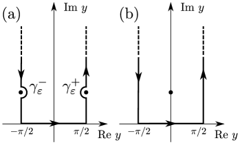
Figure 7: Integration contours in the complex $y$-plane used for the evaluation of the integral (49). The two cases correspond to: (a) $K^{\prime}>0$ and (b) $-K/4<K^{\prime}<0$.

Appendix A Decay of local perturbation

We give here further details about the calculation of the integral in Eq. (20)

$$I = \frac{\beta f}{\pi}\int_{-\pi/2}^{\pi/2}\frac{e^{2iym}\,dy}{K+4K^{\prime}\cos^{2}y}.$$ (49)

As mentioned earlier stability of the model requires that either $K^{\prime}>0$ or $-K/4<K^{\prime}<0$. We will discuss these two cases separately.

A.1 $K^{\prime}>0$

In this case the integrand has two simple poles in $y=\pm\pi/2+i\alpha$ with $\alpha>0$ the solution of $\cosh^{2}\alpha=K/4K^{\prime}$. We extend the integration over the contour indicated in Fig. 7(a), which is closed at infinity. The integral in this domain does not enclose any singularities hence it vanishes. The integrals along the two vertical lines cancel each other, due to symmetry, so one is left with

$$I+\frac{\beta f}{\pi}\int_{\gamma_{\varepsilon}^{+}\cup\gamma_{\varepsilon}^{-}}\frac{e^{2iym}\,dy}{K+4K^{\prime}\cos^{2}y} = 0,$$ (50)

where

$$\gamma_{\varepsilon}^{\pm}(\phi)=i\alpha\pm\frac{\pi}{2}+\varepsilon e^{-i\phi},$$ (51)

are the two small half-circles around the two poles. The integrations in these two domains pick up contributions from the poles and directly yield the expression (20). In particular, the oscillating behavior stems from the fact that the poles are in $\pm\pi/2$, which leads to the appearance of a factor $\exp(\pm im\pi)=(-1)^{m}$. The associated decay length is then simply given by $l_{\text{A}}=1/2\alpha$.

A.2 $-K/4<K^{\prime}<0$

In this case the integrand has a simple pole in $y=i\alpha$ with $\alpha>0$ the solution of the equation $\cosh^{2}\alpha=K/4|K^{\prime}|$. We extend the integration to the domain shown in Fig. 7(b). The integration picks up the residue from the pole along the imaginary axis. Thus, one can again obtain $I$. Note that, as the pole is purely imaginary, there are no oscillations, but a pure exponential decay.

More complicated integrands will eventually contain several poles, giving rise to a sum of exponentials. The dominant contribution will be given by the pole in the semi-infinite strip $-\pi/2\leq\text{Re}(y)\leq\pi/2$, $\text{Im}(z)>0$ which is closest to the real axis.

Appendix B Bending persistence length

The rotation operator mapping the triad $(\widehat{{\mathbf{f}}}_{k}\widehat{{\mathbf{v}}}_{k}\widehat{{\mathbf{u}}}_{k})$ into $(\widehat{{\mathbf{f}}}_{k+1}\widehat{{\mathbf{v}}}_{k+1}\widehat{{\mathbf{u}}}_{k+1})$ can be expressed as

$${\cal R}_{k}=\widehat{{\mathbf{f}}}_{k+1}\otimes\widehat{{\mathbf{f}}}_{k}+\widehat{{\mathbf{v}}}_{k+1}\otimes\widehat{{\mathbf{v}}}_{k}+\widehat{{\mathbf{u}}}_{k+1}\otimes\widehat{{\mathbf{u}}}_{k}.$$ (52)

Here $\otimes$ denotes the tensor product, which transforms a generic vector $\mathbf{a}$ as follows

$$\left(\mathbf{u}\otimes\mathbf{v}\right)\mathbf{a}=(\mathbf{a}\cdot\mathbf{v})\mathbf{u}.$$ (53)

From (52) it follows that ${\cal R}_{k}\widehat{{\mathbf{f}}}_{k}=\widehat{{\mathbf{f}}}_{k+1}$, ${\cal R}_{k}\widehat{{\mathbf{v}}}_{k}=\widehat{{\mathbf{v}}}_{k+1}$ and ${\cal R}_{k}\widehat{{\mathbf{u}}}_{k}=\widehat{{\mathbf{u}}}_{k+1}$. An alternative “axis-angle” representation uses a unit vector $\widehat{\boldsymbol{\gamma}}$ as rotation axis and a rotation angle $\theta$. For a counterclockwise rotation around $\widehat{\boldsymbol{\gamma}}$ this representation takes the form

$${\cal R}=\cos\theta\left(1-\widehat{\boldsymbol{\gamma}}\otimes\widehat{\boldsymbol{\gamma}}\right)+\sin\theta\,(\boldsymbol{\epsilon\widehat{\gamma}})+\widehat{\boldsymbol{\gamma}}\otimes\widehat{\boldsymbol{\gamma}},$$ (54)

where

$$(\epsilon\mathbf{u})\mathbf{a}=\mathbf{u}\times\mathbf{a}.$$ (55)

One can easily verify from (54) that ${\cal R}\widehat{\boldsymbol{\gamma}}=\widehat{\boldsymbol{\gamma}}$ and that for any unit vector $\widehat{\mathbf{a}}$ orthogonal to $\widehat{\boldsymbol{\gamma}}$ the following relations hold: (a) $\widehat{\boldsymbol{\gamma}}\cdot{\cal R}\widehat{\mathbf{a}}=0$ and (b) $\widehat{\mathbf{a}}\cdot{\cal R}\widehat{\mathbf{a}}=\cos\theta$. This shows that the rotated vector ${\cal R}\widehat{\mathbf{a}}$ is orthogonal to the rotation axis and that it forms an angle $\theta$ with $\widehat{\mathbf{a}}$. As mentioned in the main text tilt, roll and twist are the components of the Euler vector with respect to the local triad

$$\mathbf{\Theta}=a\tau\widehat{\mathbf{f}}+a\rho\widehat{\mathbf{v}}+a(\Omega+\omega_{0})\widehat{\mathbf{u}},$$ (56)

where its length $\Theta\equiv|\mathbf{\Theta}|$ gives the rotation angle. It is convenient to define

$$\text{t}\equiv a\tau/\Theta,\qquad\text{r}\equiv a\rho/\Theta,\qquad\text{w}\equiv a(\Omega+\omega_{0})/\Theta,$$ (57)

for which $\text{t}^{2}+\text{r}^{2}+\text{w}^{2}=1$ holds. Using (54) with $\widehat{\boldsymbol{\gamma}}=\mathbf{\Theta}_{k}/\Theta_{k}$ and $\theta=\Theta_{k}$ and (56) one finds

$$\widehat{\mathbf{u}}_{k+1} = {\cal R}_{k}\widehat{\mathbf{u}}_{k}=\left[\cos\Theta_{k}+(1-\cos\Theta_{k})\text{w}_{k}^{2}\right]\widehat{\mathbf{u}}_{k}$$ (58)

$$+ \left[(1-\cos\Theta_{k})\text{t}_{k}\text{w}_{k}+\sin\Theta_{k}\text{r}_{k}\right]\widehat{\mathbf{f}}_{k}$$

$$+ \left[(1-\cos\Theta_{k})\text{r}_{k}\text{w}_{k}-\sin\Theta_{k}\text{t}_{k}\right]\widehat{\mathbf{v}}_{k}.$$

This relation, together with the two relations obtained from $\widehat{\mathbf{f}}_{k+1}={\cal R}_{k}\widehat{\mathbf{f}}_{k}$ and $\widehat{\mathbf{v}}_{k+1}={\cal R}_{k}\widehat{\mathbf{v}}_{k}$ can be cast in a matrix product form as

$$\begin{pmatrix}\widehat{\mathbf{f}}_{k+1}\\ \widehat{\mathbf{v}}_{k+1}\\ \widehat{\mathbf{u}}_{k+1}\end{pmatrix}={\mathbf{R}}_{k}\begin{pmatrix}\widehat{\mathbf{f}}_{k}\\ \widehat{\mathbf{v}}_{k}\\ \widehat{\mathbf{u}}_{k}\end{pmatrix}.$$ (59)

The $3\times 3$ matrix ${\mathbf{R}}_{k}$ is given by

$${\mathbf{R}}=\begin{pmatrix}\cos\Theta+(1-\cos\Theta)\,\text{t}^{2}&&(1-\cos\Theta)\text{t}\,\text{r}+\sin\Theta\,\text{w}&&(1-\cos\Theta)\text{t}\,\text{w}-\sin\Theta\,\text{r}\\ (1-\cos\Theta)\text{t}\,\text{r}-\sin\Theta\,\text{w}&&\cos\Theta+(1-\cos\Theta)\,\text{r}^{2}&&(1-\cos\Theta)\text{r}\,\text{w}+\sin\Theta\,\text{t}\\ (1-\cos\Theta)\text{t}\,\text{w}+\sin\Theta\,\text{r}&&(1-\cos\Theta)\text{r}\,\text{w}-\sin\Theta\,\text{t}&&\cos\Theta+(1-\cos\Theta)\,\text{w}^{2}\end{pmatrix},$$ (60)

where for simplicity we dropped the index $k$. Setting $k=m-1$, Eq. (58) reads

$$\widehat{\mathbf{u}}_{m}=\left(\mathbf{R}_{m-1}\right)_{31}\widehat{\mathbf{f}}_{m-1}+\left(\mathbf{R}_{m-1}\right)_{32}\widehat{\mathbf{v}}_{m-1}+\left(\mathbf{R}_{m-1}\right)_{33}\widehat{\mathbf{u}}_{m-1},$$ (61)

a relation that can be iterated further using $\widehat{\mathbf{f}}_{m-1}={\cal R}_{m-2}\widehat{\mathbf{f}}_{m-2}$, $\widehat{\mathbf{v}}_{m-1}={\cal R}_{m-2}\widehat{\mathbf{v}}_{m-2}$, $\widehat{\mathbf{u}}_{m-1}={\cal R}_{m-2}\widehat{\mathbf{u}}_{m-2}$ and similar relations for $m-2$, $m-3$…. In this way one expresses $\widehat{\mathbf{u}}_{m}$ as a linear combination of $\{\widehat{\mathbf{f}}_{0},\widehat{\mathbf{v}}_{0},\widehat{\mathbf{u}}_{0}\}$ with coefficients given as products of rotation matrices (60). The tangent-tangent correlator (36) then becomes the element $33$ of the product of these matrices

$${\cal C}_{B}(m) = \left\langle\widehat{\mathbf{u}}_{0}\cdot\widehat{\mathbf{u}}_{m}\right\rangle=\left\langle{\mathbf{R}}_{m-1}\ldots{\mathbf{R}}_{1}{\mathbf{R}}_{0}\right\rangle_{33}.$$ (62)

Next, we develop two approximations for the calculation of ${\cal C}_{B}(m)$. The first one assumes that the rotation angle $\Theta$ to be infinitesimal. The second one, which is a better approximation, relies on the fact that for DNA the rotation from one basepair attached triad to the next is dominated by the intrinsic twist component.

B.1 Infinitesimal rotations

We consider the limit $\Theta\to 0$ and develop $\cos\Theta$ and $\sin\Theta$ in (60) to lowest order in $\Theta$. Formally, this can also be considered as the continuum limit $a\to 0$, which gives to lowest order (using (57))

$${\mathbf{R}}_{33} = 1-\frac{\Theta^{2}}{2}(1-\text{w}^{2})=1-\frac{\Theta^{2}}{2}(\text{t}^{2}+\text{r}^{2})$$ (63)

$$= 1-\frac{a^{2}}{2}(\tau^{2}+\rho^{2}).$$

Likewise, ${\mathbf{R}}_{13}\approx-{\mathbf{R}}_{31}\approx-a\rho$, ${\mathbf{R}}_{23}\approx-{\mathbf{R}}_{32}\approx a\tau$ and similar expressions for the other elements. We consider next the product between two rotation matrices to lowest order in $a$. For instance, for the element 13 we get

$$\left({\mathbf{R}}_{1}{\mathbf{R}}_{0}\right)_{13} = \left({\mathbf{R}}_{1}\right)_{11}\left({\mathbf{R}}_{0}\right)_{13}+\left({\mathbf{R}}_{1}\right)_{12}\left({\mathbf{R}}_{0}\right)_{23}+$$

$$\left({\mathbf{R}}_{1}\right)_{13}\left({\mathbf{R}}_{0}\right)_{33}=-a(\rho_{1}+\rho_{0})+{\cal O}(a^{2}).$$

(64)

We notice that, when calculating this product, we can set $({\mathbf{R}}_{1})_{11}=1$ and $({\mathbf{R}}_{1})_{12}=0$ as their higher order corrections in $a$ do not contribute to the lowest order in $a$ to the end result in (64). Analogously, when computing $({\mathbf{R}}_{1}{\mathbf{R}}_{0})_{23}$ we can set $({\mathbf{R}}_{1})_{21}=0$ and $({\mathbf{R}}_{1})_{22}=1$. Summarizing, if one is interested in the $33$ entry of the product of rotation matrices as in (62) to lowest order in $a$, it is sufficient to approximate a rotation matrix as

$${\mathbf{R}}_{n}=\begin{pmatrix}1&&0&&-a\rho_{n}\\ 0&&1&&a\tau_{n}\\ a\rho_{n}&&-a\tau_{n}&&1-\frac{a^{2}}{2}(\tau_{n}^{2}+\rho_{n}^{2})\end{pmatrix}.$$ (65)

The product of two such matrices (again to lowest order in $a$) gives

$${\mathbf{R}}_{1}{\mathbf{R}}_{0}=\begin{pmatrix}1&&0&&-a(\rho_{1}+\rho_{0})\\ 0&&1&&a(\tau_{1}+\tau_{0})\\ a(\rho_{1}+\rho_{0})&&-a(\tau_{1}+\tau_{0})&&X_{0,1}\\ \end{pmatrix},$$ (66)

where we defined

$$X_{0,1} = \left[1-\frac{a^{2}}{2}\left(\tau_{1}^{2}+\rho_{1}^{2}\right)\right]\left[1-\frac{a^{2}}{2}\left(\tau_{0}^{2}+\rho_{0}^{2}\right)\right]$$

$$-a^{2}\tau_{0}\tau_{1}-a^{2}\rho_{0}\rho_{1}$$

$$= 1-\frac{a^{2}}{2}\left[\left(\tau_{0}+\tau_{1}\right)^{2}+\left(\rho_{0}+\rho_{1}\right)^{2}\right]+{\cal O}(a^{4}).$$

In conclusion, the product yields again a matrix of the form (65) with tilt and roll given as the sum of the tilt and roll of the two matrices. This can be generalized to the product of $m$ matrices

$$\left({\mathbf{R}}_{m-1}\ldots{\mathbf{R}}_{1}{\mathbf{R}}_{0}\right)_{33}=1-\frac{a^{2}}{2}\left[\left(\sum_{k=0}^{m-1}\tau_{k}\right)^{2}+\left(\sum_{k=0}^{m-1}\rho_{k}\right)^{2}\right].$$ (68)

Combining this last result and Eq. (37) we get

$$\frac{1}{l_{\text{B}}}=\frac{a}{2m}\left\langle\left(\sum_{k=0}^{m-1}\tau_{k}\right)^{2}+\left(\sum_{k=0}^{m-1}\rho_{k}\right)^{2}\right\rangle,$$ (69)

which, as done for the torsional persistence length (34), in the limit $N\to\infty$ can be written as

$$\frac{1}{l_{\text{B}}}=\frac{a}{\pi m}\int_{-\pi/2}^{\pi/2}\frac{\sin^{2}my}{\sin^{2}y}\,\frac{\left\langle|\widetilde{\tau}_{q}|^{2}+|\widetilde{\rho}_{q}|^{2}\right\rangle}{N}\,dy,$$ (70)

where as in the main text $y=\pi q/N$.

B.2 Intrinsic twist dominance

An improved approximation scheme uses the fact that the rotation is dominated by the intrinsic twist component. Indeed, in DNA one has $\omega_{0}\gg|\Omega|$, $|\tau|$, $|\rho|$, where the difference is typically one order of magnitude. In degrees (note that $a\tau$, $a\rho$, $a\Omega$ are otherwise given in radians), the intrinsic twist angle is $a\omega_{0}\approx 34^{\circ}$, while the other angles are a few degrees. This suggests that one can decompose

$${\mathbf{R}}_{n}={\mathbf{S}}\widehat{\mathbf{R}}_{n},$$ (71)

as the product of two rotations where $\widehat{\mathbf{R}}_{n}$ is small and ${\mathbf{S}}$ a pure twist rotation of magnitude $a\omega_{0}$. Setting $\text{t}=\text{r}=0$, $\text{w}=1$ and $\Theta=a\omega_{0}$ in (60) we have

$${\mathbf{S}}=\begin{pmatrix}\cos(a{\omega}_{0})&\sin(a{\omega}_{0})&0\\ -\sin(a{\omega}_{0})&\cos(a{\omega}_{0})&0\\ 0&0&1\\ \end{pmatrix}.$$ (72)

The product of two consecutive rotation matrices is

$${\mathbf{R}}_{1}{\mathbf{R}}_{0}={\mathbf{S}}^{2}\left({\mathbf{S}}^{-1}\widehat{\mathbf{R}}_{1}{\mathbf{S}}\right)\widehat{\mathbf{R}}_{0}={\mathbf{S}}^{2}{\mathbf{R}}^{*}_{1}{\mathbf{R}}^{*}_{0},$$ (73)

where we defined

$${\mathbf{R}}^{*}_{n}\equiv\left({\mathbf{S}}^{-1}\right)^{n}\widehat{\mathbf{R}}_{n}{\mathbf{S}}^{n}=\left({\mathbf{S}}^{-1}\right)^{n+1}{\mathbf{R}}_{n}{\mathbf{S}}^{n}.$$ (74)

For the product of $m$ matrices we get

$${\mathbf{R}}_{m-1}\ldots{\mathbf{R}}_{1}{\mathbf{R}}_{0}={\mathbf{S}}^{m}{\mathbf{R}}^{*}_{m-1}\ldots{\mathbf{R}}^{*}_{1}{\mathbf{R}}^{*}_{0}.$$ (75)

Taking the thermal average of the $33$ component of the two sides of the previous equation we find

$${\cal C}_{\text{B}}(m)=\left\langle{\mathbf{R}}_{m-1}\ldots{\mathbf{R}}_{1}{\mathbf{R}}_{0}\right\rangle_{33}=\left\langle{\mathbf{R}}^{*}_{m-1}\ldots{\mathbf{R}}^{*}_{1}{\mathbf{R}}^{*}_{0}\right\rangle_{33},$$ (76)

where we used $({\mathbf{S}}^{m})_{3k}=\delta_{3k}$. To calculate the bending persistence length we will be using the right hand side of (76). Intrinsic twist dominance implies that in (60) $\text{w}\approx 1$ and $|\text{t}|,|\text{r}|\ll 1$ and $\Theta\approx a\omega_{0}$. We can use the approximations

$$\text{w}=\sqrt{1-\text{t}^{2}-\text{r}^{2}}\approx 1-\frac{\text{t}^{2}+\text{r}^{2}}{2}=1+{\cal O}(\text{t}^{2},\text{r}^{2}),$$ (77)

and $\Theta=a{\omega}_{0}+{\cal O}(\text{t}^{2},\text{r}^{2})$. This implies that (60) to lowest orders in t and r becomes

$${\mathbf{R}}=\begin{pmatrix}\cos(a\omega_{0})&&&&\sin(a\omega_{0})&&&&(1-\cos(a\omega_{0}))t-\sin(a\omega_{0})r\\ -\sin(a\omega_{0})&&&&\cos(a\omega_{0})&&&&(1-\cos(a\omega_{0}))r+\sin(a\omega_{0})t\\ (1-\cos(a\omega_{0}))t+\sin(a\omega_{0})r&&&&(1-\cos(a\omega_{0}))r-\sin(a\omega_{0})t&&&&1-(1-\cos(a\omega_{0}))(t^{2}+r^{2})\\ \end{pmatrix}.$$ (78)

Note that taking $a\to 0$ one recovers the infinitesimal form (65). As in that case, we can ignore terms dependent on $\tau$, $\rho$ (t and r) in the upper $2\times 2$ block as these will not contribute to the bending persistence length to significant order. Next, we calculate $\mathbf{R}_{n}^{*}$ using the above form of $\mathbf{R}_{n}$ (78) and Eq. (74). The matrices ${\mathbf{S}}^{n}$ and $({\mathbf{S}}^{-1})^{n+1}$ have a block-diagonal form as (72) and correspond to a counterclockwise twist rotation of an angle $na\omega_{0}$ and a clockwise twist rotation of an angle $(n+1)a\omega_{0}$, respectively. Equation (74) gives

$${\mathbf{R}}^{*}_{n}=\begin{pmatrix}1&&0&&-a\rho^{*}_{n}\\ 0&&1&&a\tau^{*}_{n}\\ a\rho^{*}_{n}&&-a\tau^{*}_{n}&&1-\frac{a^{2}}{2}[(\tau^{*}_{n})^{2}+(\rho^{*}_{n})^{2}])\\ \end{pmatrix},$$ (79)

where

$$\tau^{*}_{n} \equiv \frac{s_{n+1}-s_{n}}{a\omega_{0}}\,\tau_{n}+\frac{c_{n+1}-c_{n}}{a\omega_{0}}\,\rho_{n}$$ (80)

$$\rho^{*}_{n} \equiv \frac{s_{n+1}-s_{n}}{a\omega_{0}}\,\rho_{n}-\frac{c_{n+1}-c_{n}}{a\omega_{0}}\,\tau_{n},$$ (81)

with

$$c_{n}\equiv\cos(na\omega_{0}) s_{n}\equiv\sin(na\omega_{0}).$$ (82)

In the limit $a\to 0$ one has $c_{n+1}-c_{n}\sim{\cal O}(a^{2})$ and $s_{n+1}-s_{n}\approx a{\omega}_{0}$, hence $\tau^{*}_{n}\approx\tau_{n}$ and $\rho^{*}_{n}\approx\rho_{n}$ as expected. The matrix (79) is formally identical to (65) with the fields $\tau$ and $\rho$ replaced by $\tau^{*}$ and $\rho^{*}$. The bending persistence length is then given by the analogous of Eq. (70)

$$\frac{1}{l_{\text{B}}}=\frac{a}{\pi m}\int_{-\pi/2}^{\pi/2}\frac{\sin^{2}my}{\sin^{2}y}\,\frac{\left\langle|\widetilde{\tau^{*}}_{q}|^{2}+|\widetilde{\rho^{*}}_{q}|^{2}\right\rangle}{N}\,dy.$$ (83)

Using (80) and (81) the Fourier transforms $\widetilde{\tau^{*}}_{q}$ and $\widetilde{\rho^{*}}_{q}$ can be expressed in terms of the original fields. The calculation of the averages in (83) gives

$$\left\langle|\widetilde{\tau^{*}}_{q}|^{2}+|\widetilde{\rho^{*}}_{q}|^{2}\right\rangle = \frac{1-\cos(a\omega_{0})}{a^{2}\omega_{0}^{2}}\left\langle|\widetilde{\tau}_{q+\Delta q}|^{2}+|\widetilde{\tau}_{q-\Delta q}|^{2}\right.$$ (84)

$$+ \left.|\widetilde{\rho}_{q+\Delta q}|^{2}+|\widetilde{\rho}_{q-\Delta q}|^{2}\right\rangle,$$

where $\Delta q\equiv Na\omega_{0}/2\pi$ is the momentum shift associated with the double helix periodicity and originates from the Fourier transforms of $c_{n}$ and $s_{n}$ in (80) and (81). Combining (83) and (84) one obtains the expression of the persistence length (38) given in the main text.

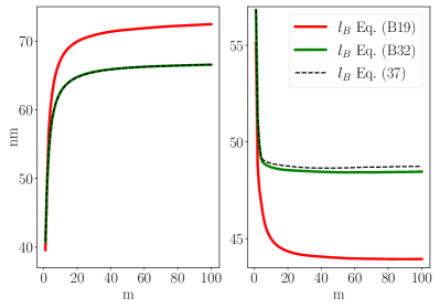
Figure 8: Monte Carlo simulations with positive (left) and negative (right) off-diagonal couplings. In both cases couplings between step-parameters up to 2 steps displaced were included. The black lines show the bending persistence length as deduced directly from the tangent-tangent correlation function (Eq. (37)). Indicated in red is the expression derived for infinitesimal rotations (Eq. (70)) and in green the improved expression (Eq. (84)).

Table 3: Parameters, given in nm, used in the Monte Carlo simulations for the calculation of $l_{\text{B}}$ shown in Fig. 8 ($X_{k}$ indicates the coupling between site $n$ and $n+k$). For the intrinsic twist density and discretization length $\omega_{0}=1.77$ nm^-1 and $a=0.34$ nm were used respectively.

		Simulation 1			Simulation 2
	$X_{0}$	$X_{1}$	$X_{2}$	$X_{0}$	$X_{1}$	$X_{2}$
$A^{t}$	60	15	5	70	-10	-5
$A^{r}$	40	8	4	60	-10	-4
$C$	80	11	3	100	-20	-5
$G$	20	2	1	30	-10	-5
$A^{tr}$	0	-2	0.5	0	0	0
$B$	0	1	0.5	0	0	0

In order to compare the quality of these approximations we employed the Monte Carlo method used in Nomidis et al. (2019b) to generate canonical ensembles of triads, distributed according to the free energy (24). In Figure (8) we compare the direct calculation of the persistence length, as deduced from the tangent-tangent correlation function (Eq. (37)), with the two approximations (Eq. (70) and Eq. (84)) for two different set of model parameters (parameters given in Table 3). In both cases the expression that takes the twist-dominance into account (Eq. (84)), yields excellent agreement with the direct calculation.

Appendix C Details all atom simulations

Using the x3dna webtool Li et al. (2019) we created an ideal B-DNA duplex structure for various oligomers of 21 and 32 basepair length. All sequences used in this work are listed in Table 4. The structure was placed in a periodic dodecahedral box with at least 1 nm distance between DNA and box boundary, followed by the addition of water and 150 mM NaCl, resulting in a charge-neutral system. Preparation of the system consisted of energy minimization (conjugate gradient with a force threshold of 100 kJ/mol nm) and a 100 ps position restrained molecular dynamics (MD) run, with restraints on the DNA heavy atoms using a force constant of 1000 kJ/mol nm in each direction. We used the parmbsc1 force field Ivani et al. (2016) to describe the interactions between atoms, in combination with the TIP3P water model Jorgensen et al. (1983). Non bonded interactions were treated with a cut-off at 1.1 nm, and long range electrostatics were handled by the Particle Mesh Ewald method. After equilibration, we performed unrestrained molecular dynamics runs at constant temperature and pressure. The velocity-rescaling thermostat Bussi et al. (2007) kept the temperature constant at 298 K and the Parrinello-Rahman barostat Parrinello and Rahman (1981) kept the pressure constant at 1 bar. All molecular dynamics simulations were performed with GROMACS version 2018.6 Abrahams et al. (2015). Frames were stored every 1 ps. The rotational degrees of freedom of the inter-basepair parameter - tilt, roll and twist - were then calculated with the Curves+ algorithm Lavery et al. (2009b). Figure 9 shows the elements of the stiffness matrix $\widetilde{M}_{q}$ for the $10$ different sequences with $N=15$ and the $3$ sequences with $N=27$ (corresponding to the $21$-mer and $32$-mer respectively), showing some characteristic sample to sample variability. The averages of these data are shown in Fig. 5(a) and (b).

Table 4: Details of the conducted simulations. N is the amount of deformation vectors $\mathbf{\Delta}_{n}$ considered per snapshot.

sequence	simulation time (ns)	N
cgcattgcatacacttggacg	1000	15
cggtaccggctctggtcgccg	1000	15
cgcgatagcgttgtctcaccg	1000	15
cgagttttgaatataagctcg	1000	15
cgggatcaggaaggtggcccg	1000	15
cgttaaagaacatctacgtcg	1000	15
cgatgggcgcggaggcagccg	1000	15
cgtcgagtaacccctaattcg	1000	15
cggcacgggacgaaatcggcg	1000	15
cgactagcatgactgtgcgcg	1000	15
cgttatgtcattataagctcaatgcttatacg	255	27
cgacgtattaccgtacgattggcactatcacg	254	27
cgaagcactgccggggatctgacatccgcgcg	174	27

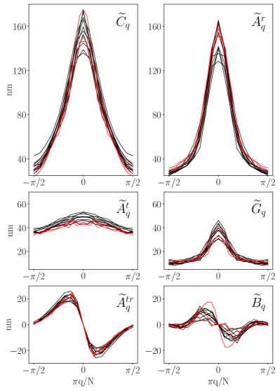
Figure 9: Entries of the momentum space coupling matrices $\widetilde{M}_{q}$ for the full spectrum of rescaled momenta for all individual simulations. Results of the $21$-mer ($N$$=$$15$) and $32$-mer ($N$$=$$27$) simulations are plotted in black and red respectively.

References

- Aggarwal et al. (2020) A. Aggarwal, S. Naskar, A. K. Sahoo, S. Mogurampelly, A. Garai, and P. K. Maiti, Curr. Op. Struct. Biol. 64, 42 (2020).
- Lankaš et al. (2003) F. Lankaš, J. Šponer, J. Langowski, and T. E. Cheatham, Biophys J. 85, 2872 (2003).
- Lankaš et al. (2000) F. Lankaš, J. Šponer, P. Hobza, and J. Langowski, J. Mol. Biol. 299, 695 (2000).
- Lavery et al. (2009a) R. Lavery, K. Zakrzewska, D. Beveridge, T. C. Bishop, D. A. Case, T. Cheatham, S. Dixit, B. Jayaram, F. Lankas, C. Laughton, J. H. Maddocks, A. Michon, R. Osman, M. Orozco, A. Perez, T. Singh, N. Spackova, and J. Sponer, Nucl. Acids Res. 38, 299 (2009a).
- Noy and Golestanian (2012) A. Noy and R. Golestanian, Phys. Rev. Lett. 109, 228101 (2012).
- Pasi et al. (2017) M. Pasi, K. Zakrzewska, J. H. Maddocks, and R. Lavery, Nucl. Acids Res. 45, 4269 (2017).
- Cleri et al. (2018) F. Cleri, F. Landuzzi, and R. Blossey, PLOS Computational Biology 14, e1006224 (2018).
- Velasco-Berrelleza et al. (2020) V. Velasco-Berrelleza, M. Burman, J. W. Shepherd, M. C. Leake, R. Golestanian, and A. Noy, Phys. Chem. Chem. Phys. 22, 19254 (2020).
- Sambriski et al. (2009) E. Sambriski, D. Schwartz, and J. De Pablo, Biophys. J 96, 1675 (2009).
- Dans et al. (2010) P. D. Dans, A. Zeida, M. R. Machado, and S. Pantano, J. Chem. Theory Comput. 6, 1711 (2010).
- Ouldridge et al. (2010) T. E. Ouldridge, A. A. Louis, and J. P. Doye, Phys. Rev. Lett. 104, 178101 (2010).
- Šulc et al. (2012) P. Šulc, F. Romano, T. E. Ouldridge, L. Rovigatti, J. P. K. Doye, and A. A. Louis, J. Chem. Phys. 137, 135101 (2012).
- Frederickx et al. (2014) R. Frederickx, T. In’t Veld, and E. Carlon, Phys. Rev. Lett. 112, 198102 (2014).
- Fosado et al. (2016) Y. A. G. Fosado, D. Michieletto, J. Allan, C. Brackley, O. Henrich, and D. Marenduzzo, Soft Matter 12, 9458 (2016).
- Skoruppa et al. (2017) E. Skoruppa, M. Laleman, S. Nomidis, and E. Carlon, J. Chem. Phys. 146, 214902 (2017).
- Chakraborty et al. (2018) D. Chakraborty, N. Hori, and D. Thirumalai, J. Chem. Theory Comput. 14, 3763 (2018).
- Li and Kabakçıoğlu (2018) H. Li and A. Kabakçıoğlu, Phys. Rev. Lett. 121, 138101 (2018).
- Skoruppa et al. (2018) E. Skoruppa, S. Nomidis, J. F. Marko, and E. Carlon, Phys. Rev. Lett. 121, 088101 (2018).
- Henrich et al. (2018) O. Henrich, Y. A. G. Fosado, T. Curk, and T. E. Ouldridge, Eur. Phys. J. E 41, 57 (2018).
- Caraglio et al. (2019) M. Caraglio, E. Skoruppa, and E. Carlon, J. Chem. Phys 150, 135101 (2019).
- Nelson et al. (2002) P. Nelson, M. Radosavljevic, and S. Bromberg, Biological physics: energy, information, life (W.H. Freeman and Co., New York, 2002).
- Lankaš et al. (2009) F. Lankaš, O. Gonzalez, L. Heffler, G. Stoll, M. Moakher, and J. H. Maddocks, Phys. Chem. Chem. Phys. 11, 10565 (2009).
- Schindler et al. (2018) T. Schindler, A. González, R. Boopathi, M. M. Roda, L. Romero-Santacreu, A. Wildes, L. Porcar, A. Martel, N. Theodorakopoulos, S. Cuesta-López, et al., Phys. Rev. E 98, 042417 (2018).
- Marko and Siggia (1994) J. Marko and E. Siggia, Macromolecules 27, 981 (1994).
- Lavery et al. (2009b) R. Lavery, M. Moakher, J. Maddocks, D. Petkeviciute, and D. Zakrzewska, Nucl. Acids Res. 37, 5917–5929 (2009b).
- Nomidis et al. (2019a) S. K. Nomidis, M. Caraglio, M. Laleman, K. Phillips, E. Skoruppa, and E. Carlon, Phys. Rev. E 100, 022402 (2019a).
- Note (1) is Hermitian because is real for every .
- Olson et al. (1998) W. K. Olson, A. A. Gorin, X.-J. Lu, L. M. Hock, and V. B. Zhurkin, Proc. Natl. Acad. Sci. USA 95, 11163 (1998).
- Srinivas et al. (2013) N. Srinivas, T. E. Ouldridge, P. Šulc, J. M. Schaeffer, B. Yurke, A. A. Louis, J. P. Doye, and E. Winfree, Nucl. Acids Res. 41, 10641 (2013).
- Schmitt et al. (2013) T. J. Schmitt, J. B. Rogers, and T. A. Knotts IV, J. Chem. Phys. 138, 01B613 (2013).
- Matek et al. (2015) C. Matek, T. E. Ouldridge, J. P. K. Doye, and A. A. Louis, Scientific Reports 5, 7655 (2015).
- Romano and Sciortino (2015) F. Romano and F. Sciortino, Phys. Rev. Lett. 114, 078104 (2015).
- Engel et al. (2018) M. C. Engel, D. M. Smith, M. A. Jobst, M. Sajfutdinow, T. Liedl, F. Romano, L. Rovigatti, A. A. Louis, and J. P. Doye, ACS nano 12, 6734 (2018).
- Desai et al. (2020) P. R. Desai, S. Das, and K. C. Neuman, Biophys. J. 118, 221a (2020).
- Chhabra et al. (2020) H. Chhabra, G. Mishra, Y. Cao, D. Prešern, E. Skoruppa, M. Tortora, and J. P. Doye, arXiv preprint arXiv:2006.15029 (2020).
- Snodin et al. (2015) B. E. Snodin, F. Randisi, M. Mosayebi, P. Šulc, J. S. Schreck, F. Romano, T. E. Ouldridge, R. Tsukanov, E. Nir, and A. A. Louis, J. Chem. Phys. 142, 234901 (2015).
- Note (2) Alternatively one can construct a global stiffness matrix and extract the real space couplings from that analysis. We verified that the results are the same.
- Note (3) Note that the coupling (7\@@italiccorr) of the toy model can also be expresses as a Fourier series (45\@@italiccorr) as follows .
- Note (4) We note that the component is The method introduced in Skoruppa et al. (2017) derived asymptotic stiffnesses using a covariance matrix obtained from the sums of , and truncated to an increasing number of terms. Hence the results reported in Skoruppa et al. (2017) report the component of the stiffness matrix.
- Lipfert et al. (2014) J. Lipfert, G. M. Skinner, J. M. Keegstra, T. Hensgens, T. Jager, D. Dulin, M. Köber, Z. Yu, S. P. Donkers, F.-C. Chou, R. Das, and N. H. Dekker, Proc. Natl. Acad. Sci. USA 111, 15408 (2014).
- Nomidis et al. (2017) S. K. Nomidis, F. Kriegel, W. Vanderlinden, J. Lipfert, and E. Carlon, Phys. Rev. Lett. 118, 217801 (2017).
- Kim et al. (2013) S. Kim, E. Broströmer, D. Xing, J. Jin, S. Chong, H. Ge, S. Wang, C. Gu, L. Yang, Y. Q. Gao, et al., Science 339, 816 (2013).
- Rosenblum et al. (2020) G. Rosenblum, N. Elad, H. Rozenberg, F. Wiggers, and H. Hofmann, bioRxiv (2020), 10.1101/2020.07.04.187450.
- Chenoweth and Dervan (2009) D. M. Chenoweth and P. B. Dervan, Proc. Nat. Acad. Sciences 106, 13175 (2009).
- Drsata et al. (2014) T. Drsata, M. Zgarbova, N. Spackova, P. Jurecka, J. Sponer, and F. Lankas, J. Phys. Chem. Letters 5, 3831 (2014).
- Singh and Purohit (2018) J. Singh and P. K. Purohit, J. Phys. Chem. B 123, 21 (2018).
- Nomidis et al. (2019b) S. K. Nomidis, E. Skoruppa, E. Carlon, and J. F. Marko, Phys. Rev. E 99, 032414 (2019b).
- Li et al. (2019) S. Li, W. Olson, and X.-J. Lu, Nucl. Acids Res. 47, W26 (2019).
- Ivani et al. (2016) I. Ivani, P. Dans, A. Noy, A. Pérez, I. Faustino, A. Hospital, J. Walther, P. Andrio, R. Goñi, A. Balaceanu, G. Portella, F. Battistini, J. Gelpí, C. González, M. Vendruscolo, C. Laughton, S. Harris, D. Case, and M. Orozco, Nat. Methods 13, 55 (2016).
- Jorgensen et al. (1983) W. L. Jorgensen, J. Chandrasekhar, J. D. Madura, R. W. Impey, and M. L. Klein, J. Chem. Phys. 79, 926 (1983).
- Bussi et al. (2007) G. Bussi, D. Donadio, and M. Parrinello, J. Chem. Phys. 126, 014101 (2007).
- Parrinello and Rahman (1981) M. Parrinello and A. Rahman, J. Appl. Phys. 52, 7182 (1981).
- Abrahams et al. (2015) M. Abrahams, T. Murtola, R. Schulz, S. Páll, J. Smith, B. Hess, and E. Lindahl, SoftwareX 1-2, 19 (2015).